U NIVERSITÀ DEGLI S TUDI DI M ILANO MASTER T HESIS Exact Out-of-Equilibrium Dynamics in Classical Integrable Field Theories Author: Giuseppe DEL VECCHIO DEL VECCHIO Supervisor: Prof. Sergio C ARACCIOLO Prof. Giuseppe MUSSARDO Co-supervisor: Dr. Andrea DE L UCA Dr. Alvise B ASTIANELLO A thesis submitted in fulfillment of the requirements for the degree of Laurea Magistrale in the Physics Department 3 th October 2019
Transcript
UNIVERSITÀ DEGLI STUDI DI MILANO
MASTER THESIS
Exact Out-of-Equilibrium Dynamics inClassical Integrable Field Theories
Author:Giuseppe DEL VECCHIO
DEL VECCHIO
Supervisor:Prof. Sergio CARACCIOLO
Prof. Giuseppe MUSSARDO
Co-supervisor:Dr. Andrea DE LUCA
Dr. Alvise BASTIANELLO
A thesis submitted in fulfillment of the requirementsfor the degree of Laurea Magistrale
in the
Physics Department
3 th October 2019
This page has been intentionally left blank...
Abstract
We study the statistical properties of the Non-Linear Schrödinger Equation (NLSE)in one spatial dimension, in out-of-equilibrium protocols and in absence of dissipa-tion, focusing on the thermodynamic limit and on states with extensive number ofparticles. On the theoretical side, integrable models exhibit exotic feautures becauseof the presence of an infinite set of conserved quantities, which strongly constrain thedynamics and offer a unique opportunity to derive exact analytical results for such anon-perturbative phenomenon as equilibration. Moreover, this extensive set of chargesbreaks down ergodicity and, being the system closed, leads to relaxation towards theso-called Generalized Gibbs Ensemble (GGE)[1]. Experimental advances in the realmof ultra-cold atom systems have boosted the theoretical interest in such special mod-els[2]. In this setting, the out-of-equilibrium properties have been extensively probedin the framework of the famous quantum quench[3–5] and the Lieb-Liniger model (LL)has received particular attention. It describes a system of massive bosons with contactinteractions and it is the quantized version of the NLSE. There are several reasons mo-tivating our research. Firstly, the NLSE can be viewed as the semiclassical limit of theLL model, that is the regime of high occupation numbers and so it can provide newinsights about its quantum counterpart, resulting in an array of results which mightbe amenable to experimental tests [6, 7]. Secondly, classical systems are faesible of ex-tensive numerical simulations, which are not possible for the quantum LL. Thirdly, wehave at our disposal many theoretical tools developed for the LL model which we canuse in a rather economic way in order to access similar information of the NLSE, aftersuitable semiclassical limit[8]. Specifically, the purpose of this thesis is to study the clas-sical counterpart of the homogeneous quantum quench, through the exploration of therelaxation properties of the system and the determination of the emergent steady state,once the initial conditions are given. This goal will be achieved by merging theoreti-cal techniques, such as the Inverse Scattering Method and Bethe Ansatz, and numericalcomputations for the transfer matrix, the latter encoding all the relevant information ofthe steady state[9]. In particular, we give exact analytic expressions for the full count-ing statistics of the particle density and its moments. Our findings are valid for thesteady state coming from arbitrary conditions. Besides out-of-equilibrium setups, theseformulas can be applied to equilibrium thermal states as well.
Acknowledgements
Le prime persone che vorrei ringraziare sono i miei professori, Sergio Caraccioloe Giuseppe Mussardo. Il professor Caracciolo per i suoi insegnamenti e per l’immensafiducia datami durante questi anni di studio e il professor Mussardo per avermi invitatopresso la SISSA, dove questo progetto si è sviluppato, e per avermi accolto con infinitaospitalità. Ringrazio Alvise Bastianello, per me Alvi, per essere stato presente 24 ore algiorno 7 giorni su 7: senza di te tutto ciò non sarebbe stato possibile. Ringrazio AndreaDe Luca, per gli inestimabili consigli tecnici e non. Ai miei genitori dico che tutto quelloche avete fatto per me non si può ringraziare, si porta nel cuore. Ringrazio le mie sorelle,Jasmin e Luisa per essermi state vicine anche nei periodi peggiori, senza di voi nonsarei la stessa persona. Non ringrazierò i miei amici esplicitamente: l’amicizia è ciò chedi migliore ho trovato duranti i viaggi di questi anni. Le cose grandi si fanno sempreinsieme, per questo, senza di voi non ce l’avrei mai fatta. Infine, ringrazio A. per avermiinsegnato che un sorriso ti cambia la giornata e per avermi supportato durante l’ultimosforzo.
Quantum physics has been, since its birth, an industry of astonishing experimental re-sults. On the other side, theorists, provided an array of models based of very few andphysical assumptions, but neverthless able to explain such an non-intuitive quantummechanical behaviour of Nature. Few decades before, Boltzmann, alone, gave rise to thebranch of theoretical physics studying a large number of degrees of freedom based onprobabilistic methods. The Hydrogen and Helium atoms spectrum were fully describedand predicted by the quantum theory but as happend in classical physics the three bodyproblem represented soon an insormountable difficulty: the problem of many bodyquantum systems was knocking at the doors. Applying Boltzmann ideas to quantumsystems showed up in a fruitful extension of thermodynamics to the microscopic world.New and spectacular phenomena were supposed, observed and predicted like the Bose-Einstein condensation (BEC). The basic assumption of equilibrium statistical mechanics(ESM) is the so-called ergodic hypotesis, now a theorem in many instances [10, 11]: ba-sically, through the entire time evolution of the system, it densely visits each region ofphase space. The hypotesis directly allows to postulate, according to Boltzmann [12],the a priori equal probability for each state of the system. The important point is thata generic system, quantum or classical, is described by the Gibbs distribution at equi-librium, p(E) = e−βH: we call this distribution thermal state. Physically, the process ofthermalization happens because of the presence of non linear terms in the equationsdescribing the evolution, so that they induce non trivial scattering processes betweenparticles (or interactions between degrees of freedom) such that there is a consequentmixing of modes, leading ultimately to thermalization: in weakly interacting models,this simply means energy is shared equally by each normal mode of the unperturbedHamiltonian. In turn, this implies that the potential energy has been transformed intokinetic energy. We will see, that for field theories, the responsible player of utlimatethermalization is the laplacian term appearing in the equations of motion. Generallyspeaking, there are two main paradigms to describe a certain system: one can use a"fundamental" description and take into account every degree of freedom by which thesystem is made and eventually take the thermodynamic limit; the second approach isthat of a field theory. The aformentioned descriptions are often interchangable and thechoice depends on the system at hand but it is worth to say that there are phenomenathat needs to be necessarily described by field theories: the most outstanding example isthe Standard Model. However, switching between continuum and discrete models doesnot come without a price. Field theories suffer from UV divergences, a situation bestrepresented by the UV catastrophe which led to the development of quantum mechan-ics. The Wilson renormalization group [13] has pushed forward our understanding ofthe divergences: it gave us a practical tool to cure them and to understand whether thisis possible or not. Through a coarse grain procedure it is possible to sum up short wavelength modes unimportant in low energy physics and incorporate the contribution inthe parameters defining the model. Another important aspect of field theories is that
2 Contents
of symmetry. Indeed, modern theories are built up by lagrangians with an underlyingsymmetry group, which can be local, like for gravity, or global like for electrodynam-ics. The mechanism of spontaneous symmetry breaking [14] represents a cornerstone inthis respect and permitted to explain the existence of massive particles and magneticsmaterials. Thus, it should clear that the field-theoretic paradigm has been fundamentalin our description of Nature. Neverthless, it still deserves attention in many aspectsas we want to show. Our present study is devoted to the out-of-equilibrium dynamicsof classical integrable field theories and we will adopt the field-theoretic point of view forthe most part of the thesis. Integrability is a fascinating subject and a rare property ofa system: a complicated theory, like non-linear partial differential equation or a many-body quantum system, in special cases, turns out to be exactly solvable. This happensbecause, despite the appearence, there is a large number of, mostly hidden, symmetrieswhich reduce the effective ways a system can evolve. Integrability and solvability areoften used as synonymous but actually the precise meaning of each concept needs care-ful clarification and only after that their connection can be understood. There are manyreviews and books at different levels which discuss in deep the meaning of integrabilityin different context, namely quantum systems and classical ones. Here, we refer to Ref.[15] for integrability from a classical point of view and to Ref. [16] for quantum case.Despite exactly solvable models are rare they neverthless have a special role in our un-derstanding many non-perturbaitive phenomena. Real-life phenomena seem to comeout from very complicated and random interactions between many different degrees offreedom. For instance, in a many-body interacting system, from an excess of internal en-ergy in the system, trilions of scattering events between molecules are generated and sochaotic motion. If we let the system evolve subject to its own interactions only, we willsee that, after a reasonable amount of time, it will equilibrate to a steady state: we saythat the system has reached thermodynamic equilibrium. Traditionally, the approach tomany-body complicated systems has seen three different lines of research:
• Approximation schemes
• Perturbation theory
• Numerical Methods
For example, in a typical condensed matter system, electrons interact with each otherand with ions on a lattice. The Hartee-Fock approximation is a mean field equation whichconsiders each electron as independent, moving in the average potential created by theother electrons. In this approximation ions are considered frozen on the lattice. Instead,if one wants to study vibrational properties of the solid, one can consider oscillationsof the ions around their equiilbrium positions. The first approximation is to treat themas classical particles, so harmonic oscillators, and compute variuos natural frequencies.The next step is to quantize the oscillators and study their dispersion relations. Thisleads to the concept of phonons. Following this way electrons may play no role, at leastat the beginning, but as we take them into account interesting phenomena may occur:a celebrated example is superconductivity, explained in terms of electrons-phonons in-teraction [17]. On the other side, perturbation theory has reached a certain level ofmaturity. Applications of this powerful technique range from particle physics to many-body physics. Despite this, there are a number of drawbacks in using and interpretingperturbation theory. First, there are phenomena that are intrinsecally non-perturbative:
Contents 3
out-of-equilibrium physics and topological physics are two simple examples. Second,mathematically we get power series exapansions which are generically divergent: thebest we can do is to interpret them as asymptotic series. Moreover, today we have at ourdisposal an incredible set of high-performance computational tools. Even smartphoneshave computational power far higher than an IBM computer had in the seventies. Newnumerical methods are coming out: the density renormalization group, exact diagonal-ization, tensor networks and so on [18]. Unfortunately, in many cases, the complexityof macroscopic systems (mostly the quantum ones in d > 1) prevents any straightfor-ward application of the aformentioned methods due to entanglement effects (citation).Having said all of that, it is clear that the search and the understanding of integrablemodels is an important task in modern physics, since it can ultimately give us very use-ful insights on how interacting many-body systems behave exactly. It is not sufficient,for a true understandig of strong coupling regimes, to exclusively rely on approximateschemes. In addition, a theorem by Liouville [15, 19] ensures that the dynamics of in-tegrable theories is profoundly different with respect to that of non-integrable ones andis reduced to oscillations because they have as much conserved quantities as degrees offreddom. In the thermodynamic limit the situation is similar as the number of conservedcharges becomes extensive. Understanding the exact dynamics of integrable theorieswould provide a comprehension of exact behavior of fully interacting models, withoutapproximations or numerical errors. Put in this way it could seem that the interest instudying integrable models is purely theoretical: this is definitely wrong. On the clas-sical side, integrable field theories arise in many different areas: the Kortweg-deVriespartial differential equation describes solitary waves in shallow water, magnetohydro-dynamics waves and long waves in anharmonic crystals; the Non-Linear-SchrödingerEquation (NLSE) instead, which, by the way, will be our playground model to test ex-act predictions, appears to describe homogeneous BEC systems [20, 21] and solitons infiber optics [6]. In 1955, in Los Alamos Laboratories, Fermi, Pasta and Ulam investi-gated the approach to equilibrium in an anharmonic chain. The experiment showedthat, for initial configurations peaked on low energy sector, quasi-periodic motion wasa rule rather than an exception and it seemed to the authors that there was a lack ofthermalization, an unexpected situation due to the non-integrability of the system. Thiscan be put in the context of the KAM theorem [22] which allows for quasi-periodic mo-tion in presence of small integrability-breaking terms. However, KAM theorem holdswell for systems with finite degrees of freedom and it is not directly applicable in thethermodynamic limit. Later, the situation of the FPU paradox was better explained byKruskal and Zabusky [23] who recognized that the low energy sector of the FPU modelis well captured by the KdV equation. Thus, for very long times integrability of KdVbreaks down and non-integrable sector of FPU model kicks in, making the system ther-malize. In the quantum world a breakthorugh experiment was performed in 2006, whenKinoshita et al. investigated the equilibration properties of a BEC system varying its di-mensionality d [2]. In one dimension this can be depicted as the quantum version of theNewton’s Cradle as illustrated in Figure 1. They found that the equilibration properties ofa one dimensional system of 37Rb bosons is completely different with respect to higherdimensions. Indeed, in d = 2, 3 the system thermalized as expected, but in d = 1 it didnot. The reason was attributed to approximate conservation laws in the model. Indeed,the famous Lieb-Liniger model (LL) [24, 25] nicely fits with the experimental realizationof the bosonic system with repulsive contact interactions, despite the presence of the
4 Contents
FIGURE 1: (a) Classical Newton’s Cradle. (b) Pictorial representation ofout-of-equilibrium time evolution of trapped 1d BEC considered in [2]. Onthe right, absorption image of the same time evolution. Figure taken from
the same reference.
trapping potential which weakly spoils exact integrability. These kind of experimentsare nowdays continuously performed in laboratories, allowing the study of non equilib-rium dynamics of nearly isolated quantum systems. The theoretical paradigm throughwhich we explore this phenomenon is the quantum quench [3–5], a protocol which hasbeen successfully applied to a lot of many-body systems. To explain the protocol, con-sider a Hamiltonian H(g) depending on a parameter. At t < 0, one prepares the systemin the ground state |ψ0〉 of H(g0) with g 6= g0, in such a way that the system is notin an eigenstate of H(g) (and therefore exhibits non trivial evoution), displaying at thesame time well defined physical properties like extensivity and the cluster decompo-sition property. At t = 0 the parameter is suddenly changed to another value g andthe state evolves according to H(g). Then, one is interested in computing steady stateproperties of local observables [26], namely the t → +∞ limit. In the Bogolioubov ap-proximation, the NLSE describes the dynamics of a homogenous BEC in the ground state[27, 28]. Indeed, handling the semi-classical limit of the LL model amounts to considerthe field operator ψ as a classical quantity. Also, in the ground state of the BEC there isa macroscopic number of particles, so that field operators of this state are of order
√N
and one can ignore their non-commutativity. Thus, studying the out-of-equilibriumproperties of the NLSE would provide useful information both on the behavior of thequantum system in such a regime and on the dynamics of the equation itself. The ques-tion on the equilibration properties of classical integrable field theories in general hasbeen analyzed in [9] in the context of the Sinh-Gordon model (ShG) [29]. This model isalso integrable and contains only one bosonic massive particle, rendering its study rela-tively simple. In the former reference, the authors considered the 1+ 1 dimensional ShG
Contents 5
equation with initial conditions far-from-equilibrium and extensive total energy. Thishas been achieved enforcing periodic boundary conditions and populating only shortwavelength modes of the initial configuration. On one hand, it is well known that quan-tum integrable models are solvable by means the Thermodynamic Bethe Ansatz [30, 31],which permits the computation of thermodynamic quantities at equilibrium. On theother side, there is a longstanding tradition in mathematical physics community study-ing classical integrable field equations [32–34] as a complete theory for such models hasbecome well estabilished: this is called Inverse Scattering Method (IST). Subtleties arisewith periodic boundary conditions, since the method is supposed to work when fieldsare rapidly vanishing at infinite distance. The expression for the solution in the thermo-dynamic limit becomes impossible to use: this is the infinite gap solution. An importantpoint of Ref. [9] is that they rised the idea to use the solution of the full quantum prob-lem and a semi-classical limit h → 0 to access quantities in the corresponding classicaltheory: Form Factors theory [35, 36], TBA and the LeClaire-Mussardo formula valid in[37] and out of equilibrium [38], allow to compute steady-state averages of meaning-ful physical quantities, like the trace of the stress-energy tensor or the vertex operators.Albeit extremely useful, the LeClaire-Mussardo in an expansion and an exact resum-mation is extremely difficult. On the other hand, new results in the quantum LL modelgive access to several physical observables by means of closed and exact expressions.The merit of the above paper is that the authors linked the IST to TBA. Indeed, deter-mining the effective temperatures of the Generalize Gibbs Ensemble (GGE) [39–41]is atremendous task. However, a huge step forward can be made once one recognizes thatan equivalent amount of information is contained in the transfer matrix coming from theIST. Once this information has been extracted, numerically for example, it is possibleto solve the TBA equations in the semi-classical limit. In Ref. [8, 42] a step forwardthe computation of one point functions 〈(ψ†(x)ψ(x))K〉 in the LL model has been done:to access the steady state properties they do not use the LeClaire-Mussardo expansion,rather a combination of the recently conjectured Negro-Smirnov formula, which givesthe expectation values of vertex operators in the ShG model in arbitrary macrostates[43–45]and can be applied to the quantum LL after a proper non-relativistic limit [46,47]. At this point it should be clear that we have at our disposal several results bothin the quantum setting and in the classical one. Exploiting the knowledge of one pointfunctions in the LL model we can compute the same quantities for the NLSE, after thesemi-classical limit. We go further: in [8] the full counting statistics (FCS) for the numberof particles in a small interval has been computed, but the applicability is limited to avery tiny inteval. The FCS is rather important from the experimental point of view, sinceit let us compute probabilities of outcomes of a given measure, not just its average valuein the classical realm. We calculate exactly the FCS in the steady state through exploitingagain the non-relativistic and semi-classical limit of the Negro-Smirnov formula. Ourresult is valid on equilibirum thermal states and arbitrary GGEs as well, opening thepossibility to study the FCS on steady states following arbitrary quenches. Since ourmodel is classical we have the possibility to chek our analitycal calculations using ex-tensive numerical simulations, an impossible task in the quantum setting. The theisis isorganized as follows. In Chapter 1 we introduce the concept of integrability in classicalmechanics both for systems with finite and infinte degrees of freedom. In particular,we discuss integrable field theories in relation with statistical physics applications andfree theories will provide the simplest models displaying non trivial character and most
6 Contents
of the their characteristic will remain in interacting models. Indeed we will se here theLieb-Liniger model and the coordinate Bethe Ansatz solution leading a quasiparticlesdescription of its Hilber space. Lastly, we introduce the semiclassical limit of quantumfields. In Chapter 2 we explain the problem of relaxation and thermalization in classicalintegrable field theories. The quench protocol is introduced and applied to the rela-tivistic bosonic free field as an example of non trivial properties of out-of-equilibriumphysics of integrable theories. Initial conditions are discussed and it is shown that ifthe latters are analytic we can make some quantitative prediction about the time scalesinvolved in the process of equilibration. Moreover, the Thermodynamic Bethe Ansatzis deeply reviewed and its semiclassical limit is presented on the grounds of the Lieb-Liniger model: this will serve as a basis for our future calculations. Chapter 3 is devotedto the review of the Inverse Scattering Method, a powerful analytical tool used to findsolutions to a class of certain non linear partial differential equations. The method willprovide an infinite set of conserved quantities in the the Non Linear Schrödinger model,proving its integrability and, more importantly, will allow us to identify the relevantquantity, the root density, which characterize uniquely the steady state. An importantpoint here, is the relation between the problem defined on the whole line and tha onedefined on the circle (period boundary conditions). Chapter 4 is where we compute thefull counting statistics for the number of particles and the density one point correlationfunctions. We present the non relativistic limit of the Sinh-Gordon field theory, resultingin the quantum Lieb-Liniger model. This fact sets up a mapping between the two the-ories and consequentely a correspondence between their field contents. The full contigstatistics is computed by means of a combination of the non relativistic and semiclassicallimits of a formula due to Smirnov and Negro allowing the computation of vertex oper-ators in the Sinh-Gordon model. The last chapter is devoted to the numerical recipes wehave implemented to compare analytical predictions with direct numerical simulationsof the Non Linear Schrödinger equation in out-of-equilibrium conditions.
7
Chapter 1
Integrable Models
In this Chapter we briefly review the main ingredients of the theory of classical systemswith finite degrees of freedom. A formulation of mechanics based on symmetries isnatural to show these ideas at work, so the Hamiltonian formulation is the preferredchoice. We beign with basic concepts of Hamitlonian mechanics, like canonical tranfor-mations and action-angle variables for simple one dimensional systems. We state andprove Liouville’s definition of integrability. We discuss the celebrated KAM theoremand show why it is not directly applicable in the thermodynamic limit. After, we givethe idea of why a precise definition of integrability in the quantum setting is still miss-ing. We discuss the role of scattering in integrable models and introduce the conceptof S- matrix, as the analytic linear transformation encoding all the properties of scatter-ing, especially in d = 1 + 1 models. Finally, we introduce a classical integrable modelswhich will play an important role in this thesis: the non-Linear Schrödinger model to-gether with its quantized versions, the Lieb-Liniger model. Morover, we will enlightenan important relation between the famous Sinh-Gordon model [29] and the Lieb-Linigermodel. Indeed, the Lieb-Liniger model can be regarded as the non-relativistic limit ofthe Sinh-Gordon.
1.1 Classical Integrability
1.1.1 Finite Number of Degrees of Freedom
In classical mechanics the mathematical description of a physical system is rather sim-ple. We describe a system with N degrees of freedom by two sets of canonical coordi-nates (qi, pi) ∈ ΓN. We will use bold letters to indicate sets of quantities: for instance,q stands for all the coordinates qi. A dot indicates the time derivative. The set ΓN isa differentiable manifold and is called phase space. It is always of even dimension 2N.With respect to the Lagrangian formualation, the doubling of independent coordinatesis a worth price to pay in favour of a theory based on symmetries. For a system withHamiltonian H(q, p), the equation of motion take the form,
q =∂H(q, p)
∂pp = −∂H(q, p)
∂q(1.1)
The phase space is promoted to a symplectic manifold with the introduction of the Pois-son brackets defined for each pair of observables F and G as,
F, G =N
∑i=1
(∂F∂qi
∂G∂pi− ∂F
∂pi
∂G∂qi
)(1.2)
8 Chapter 1. Integrable Models
Indeed, we call observables every differentiable function F : ΓN → R and from the formof equations of motion it soon follows that the time evolution is generated1 by the Hamil-tonian,
f = f , H (1.3)
Equivalently it is possible to define a non-degenerate 2-form Ω = ∑Ni=1 dqi ∧ dpi acting
on vector fields as,Ω(X, Y) = X, Y (1.4)
Every pair of observables satisfying,
F, G = 1 (1.5)
is said to be a canonical pair. Clearly, (qi, pi) is a canonical pair for every i. If the Pois-son bracket between two obervables vanishes we say that they commute. An impor-tant point of this way of writing the evolution equation for an observable is that everytime it commutes with the Hamiltonian is a constant of motion. The set of observablesequipped with the pointwise sum of functions and the scalar multiplication by a realnumber becomes a vector space. The introduction of the Poisson bracket is known asLie Algebra. It satisfies the three basic properties of a Lie product,
A coordinate transformation between a canonical set of coordinate (q, p) and anothercanonical set (Q, P) is said to be canonical. In other words, canonical transformationspreserve the hamiltonian structure of the equations of motion. As we said above, theHamiltonian formulation is more natural to make symmetries explicit. To illustrate thispoint, without loss of generality, consider a generic observable for a one dimensionalsystem f = f (q, p) and an infinitesimal translation, q 7→ q + ε. It follows that,
δ f = f (q + ε, p)− f (q, p) = ε∂ f∂q
+ O(ε2) (1.6)
Now consider the following Poisson bracket,
f , exp (εp) = f , 1 + εp + O(ε2) = ε∂ f∂q
+ O(ε2) (1.7)
By comparison it follows that
δ f = ε f , p+ O(ε2) (1.8)
In this sense the momentum generates infinitesimal translation. Also, infinitesimaltranslations are canonical. In the very same way the Hamiltonian generates time trans-lations. The argument above in just a particular example of a more general formalism
1This is the deep meaning of what is meant by symmetry.
1.1. Classical Integrability 9
based on what are called generating functions. Consider, again for simplicity, a one di-mensional Hamiltonian H(q, p), where (q, p) are canonical variables. Equations of mo-tion can be derived from the Hamilton’s principle
δ∫ t2
t1
(pq− H(q, p)) dt = δ∫ t2
t1
(PQ− K(Q, P)
)dt = 0 (1.9)
which holds when variations at end points are zero. This means that2,
pq− H(q, p) = PQ− K(Q, P) + F (1.10)
The function F is called generating function of the canonical transofmation and it candepend on any combination of old and new canonical coordinates. For example if F =F1(q, Q, t) we have,
pq− H(q, p) = PQ− K(Q, P) +∂F2
∂qq +
∂F2
∂pp +
∂F2
∂t(1.11)
The above relation can hold only if we identify,
p =∂F2
∂q(1.12)
P = −∂F2
∂p(1.13)
H = K +∂F2
∂t(1.14)
If we want to consider F = F2(q, P, t) the Legendre transform is the answer,
F2(q, P, t) = F1(q, Q, t) + PQ (1.15)
p =∂F2
∂q(1.16)
Q =∂F2
∂P(1.17)
Of course there exist other types of generating functions. The Hamilton-Jacobi methodof action-angle variables consists in finding a particularly simple set of canonical coor-dinates: the ones which stay constant in time. For this choice, Hamilton’s equationsare,
Hence, the new Hamiltonian must not depend on coordinates at all. If we choose K = 0from (1.14) we get an equation for F,
H(q, p, t) +∂F∂t
= 0 (1.20)
Further, if we take F = F2(q, P, t) from (1.16) we discover the Hamilton-Jacobi equation,
H(
q,∂F2
∂q, t)+
∂F2
∂t= 0 (1.21)
It is customary to rename F2 = W. In the literature this is known as Hamilton’s char-acteristic function. Now if the system is time-translation invariant the Hamiltonian isconserved,
H(q, p) = α1 (1.22)
and solving for p we find p = p(q, α1). Thus, the integral,
J(α1) =∮
pdq (1.23)
depends only on α1. This is called action variabale. The integration is extended over anentire period of the motion. Solving for α1 we can write,
H = H(J) (1.24)
The Hamiltonian is function only of the action variable. The conjugate variable ω iscalled angle. The name comes from the fact that this quantity is connected to the freqe-uncy of rotation or libration of the system,
ω =∂W∂J
(1.25)
for the Hamilton’s equation are,
ω =∂H∂J
= v(J) (1.26)
This is easily solved,ω(t) = v(J)t + β (1.27)
To makes explicit connection with the frequency (or the period) we compute,
∆ω =∮
∂ω
∂qdq =
∮∂2W∂q∂J
dq =ddJ
∮∂W∂q
dq =ddJ
∮pdq = 1
But we know how ω evolves in time so,
∆ω = v(J)T = 1 (1.28)
1.1. Classical Integrability 11
That is,
T =1
v(J)(1.29)
are the oscillation periods. This can be done if the system is doing periodic motion inphase space, since otherwise we can’t define
∮-integrals. This is true for an harmonic
oscillator, but not for a free particle.
1.1.2 Liouville Integrability and KAM theorem
Having recalled basic concepts of Hamiltonain mechanics for systems with finite de-grees of freedoms, we give with the definition of integrability due to Liouville,
Definition 1. (Liouville integrability) A system with N degrees of freedom is said to be inte-grable if it has N independent conserved quantities in involution,
Fi, Fj = 0 (1.30)
Independence here means that the set defined by the simultaneous conditions Fi = fi ∈ R,i = 1, . . . , N define an N dimensional sub-manifold of the phase space Γ f
N.
Posed in this way, the definition of integrable system in the classical context is clear.It suffices to find a system of conserved charges in number equal to the degrees of free-dom and in involution (in the above sense) to estabilish integrability. The meaning ofthe existence of such a system of charges is that the dynamics is constrained by the con-servation laws. The bijection between conservation laws and degrees of freedom is sostringent that the system can be solved by quadratures. Indeed we have the followingtheorem [19],
Theorem 1. (Liouville) The solution of the equations of motion of a Liouville integable systemcan be obtained by quadratures.
Solvability means that, instead of solving directly the equations of motion, whichin are in general PDEs, we can find a change of coordinates such that the dynamicsbecomes simple (trivial). By quadrature means that we have to solve a finite number ofintegrals. The idea behind the theorem is exactly the one described for the Hamilton-Jacobi method of action angle variables. One passes from a set (q, p) to a new set ofcanonical coordinates (F, Ψ) still satisfying,
Fi, Ψj = δij (1.31)
which trivialize the dynamics according to (1.18)-(1.19). The proof of Liouville’s theo-rem is easy and we report it hereafter [15].
Proof. Define the canonical 1-form as α = ∑i pidqi and the symplectic 2-form (equivalentto the existence of a Poisson bracket structure on the phase space) as Ω = dα = ∑i dpi ∧dqi. The task is to construct a canonical transformation (qi, pi) → (Fi, Ψi) such that theFi are among the new coordinates:
Ω = ∑i
dpi ∧ dqi = ∑i
dFi ∧ dΨi
12 Chapter 1. Integrable Models
To construct the transformation we build up its generating function. Let Γ fN the level
manifold of the phase space Fi(q, p) = fi and suppose that we can solve these relationsfor pi. Consider the function,
S(F, q) ≡∫ m
m0
α =∫ q
q0∑
ipi( f , q)dqi (1.32)
where the integration path is drawn from Γ fN and goes from the point m0 = (p(f, q0), q0)
to the point m = (p(f, q), q) where q0 is some reference value. Assume the existence ofS. It follows that we can define,
Ψi =∂S∂Fi
and we have,
dS = ∑i
ΨidFi + pidqi
Since d2S = 0 we find Ω = ∑i dpi ∧ dqi = ∑i dFi ∧ dΨi. This proves that S is well-definedand the transformation canonical. To prove that such an S exists we must show that itis not dependent on the integration path. By Stokes theorem, we need,
dα|Γ f
N= Ω|
Γ fN= 0
To do this one consider the vector field associated to Fi defined by dFi = Ω(Xi, ),
Xi = ∑j
∂Fi
∂qj
∂
∂pj− ∂Fi
∂pj
∂
∂qj
These vector fields are tangent to the level manifold Γ fN because of Liouville integrabil-
ity,
Xi(Fj) = Fi, Fj = 0
Since Fi are assumed to be independent this tangent space is well defined. Also Ω(Xi, Xj) =dFi(Xj) = 0 and we have proved that Ω|
Γ fN= 0.
Having recalled and proved the Liouville’s theorem we now discuss the KAM theo-rem in a simplified manner, in order to avoid technical detours which exile the purposesof this thesis. This classical theorem concerns with the stability of motions in hamil-tonian systesm that are small perturbations of integrable ones. They are genericallydescribed by Hamiltonians of the type,
H = HI + εV (1.33)
where HI is an integrable Hamiltonian while ε is the strenght of the perturbation. Be-fore KAM theorem, it was believed that resonant tori in the phase space are destroyed
1.2. Integrable Field Theories 13
by arbitrairily small perturbations. If HI is integrable it depdens only by the action vari-able defined in the previous section, HI = HI(J), with J ∈ D ⊂ RN. UnperturbedHamilton’s equation are readily integrated to give,
J = J0 ω(t) = ω0 + v(J)t
with ∂JW = ω ∈ [0, 2π] is the angle variable and S is the Hamilton’s characteristicfunction. The geometry of the flow of an integrable system is thus described as peri-odic cycles on an n-dimensional torus TN with periods given by (1.29). One shouldnot forget that the original coordinates are related to the action-angle ones by a certaintransformation, but the motion is anyway periodic in the angle variables. Thus, it ispossible to expand the solutions in Fourier series and they will be of the form,
∑k∈ZN
ak(J)ei(〈k,ω0〉+t〈k,v(J)〉) (1.34)
As a consequence, the motion is quasi-periodic in t (〈, 〉 denotes the usual scalar productand we are meaning vector quantities). The frequences of the motion can be of twotypes [48],
• Non-resonant or rationally independent 〈k, v(J)〉 6= 0 for all k 6= 0 ∈ ZN
• Resonant or rationally dependent 〈k, v(J)〉 6= 0 for some k 6= 0 ∈ ZN
When one considers the perturbed Hamiltonian H, it can be proven that the majorityof tori survives. Not only their frequencies are resonant but strongly resonant, meaningthat there exist constants α > 0 and τ > 0 such that,
|〈k, v〉| ≥ α
|k|τ ∀0 6= k ∈ ZN (1.35)
with |k| = ∑i |ki| where i ranges over the number of frequences (for a multi-frequencymotion). This condition is called diophantine or small divisor condition. The KAM theo-rem states the stability of invariant tori provided that,
|ε| < δα2 (1.36)
for some δ > 0. It is clear that, since k’s are integers, as we take the thermodynamiclimit the above bound vanishes and the theorem loses its validity. For what concernsthe dynamics of field theories we cannot realy on any precise mathematical theory as theKAM theoy. Studies are based uniquely on numerical methods and for what concernsintegrable models on the Inverse Scattering Transform.
1.2 Integrable Field Theories
I the Fifties it has been recognized that a theory of fundamental interactions is best builton Lagrangians supporting infinite degrees of freedom. This led to the developmentof quantum electrodynamics and later, with the introduction of local gauge invariance,models for the weak and strong interactions. Before that, there were at least two im-portant physical models based on the field theoretic paradigm, namely the theory of
14 Chapter 1. Integrable Models
General Relativity and Maxwell’s Electrodynamics. Soon, the field theoretic point ofview was extendend to the description of condensed matter systesms, an incrediblearena of unexplained phenomena to test this languange. Like in classical or standardquantum mechanics, each model is specified giving a Lagrangian or a Hamiltonian, thistime depending on an infinite number of degrees of freedom. The main guiding line forthe construction of such models has been the symmetry principle: in short, each systemis characterized by a particular set of symmetries and one builds up the Lagrangian (orbetter the Action) having the same symmetries. Thanks to Noether’s Theorem, for eachsymmetry there are associated conserved charges. These charges can be usually derivedfrom an integral over a local density, which in turn is the first component of a currentsatisfying a continuity equation. Our focus is on a particular class of field theories whichwe call integrable. At the very primitive level we will see that these theories display aninfinite set of conserved charges.
1.2.1 Prototype of Integrable Field Theory: free models
Non Relativistic Free Field
As one of the simplest field theories one can conceive, we present the free theory of asingle complex bosonic field ψ(x, t) in 1 + 1 dimensions ruled by the Hamiltnoinan,
H =∫H(ψ, ψ)dx =
∫|∂xψ(x, t)|2dx (1.37)
and Lagrangian,
L =∫L(ψ, ψ)dx =
∫ i2(ψ∂tψ(x, t)− ψ∂tψ(x, t))− |∂xψ(x, t)|2
dx (1.38)
The integration is over the real line for fields vanishing at infinity or over a period forperiodic fields. The Poisson structure is given by the following bracket,
ψ(x, t), ψ(y, t) = iδ(x− y) (1.39)
with the vanishing of the remaining brackets. This is because the canonical momentumassociated to the variable ψ is,
π(x, t) =∂L
∂(∂tψ)= iψ(x, t) (1.40)
The field equation corresponding to this theory is the free-particle Schrödinger equa-tion,
i∂tψ(x, t) = −∂2xψ(x, t) (1.41)
For the moment we do not specify boundary conditions for this equation. From now,it is understood tha the field depends always on t as we will display only the spatialcoordinate for notational simplicity. Despite this theory may seem very simple sincethere is no interaction, it neverthless displays many of the concepts that we will find innon trivial interacting models. In is easy to show that in this theory there are at least
1.2. Integrable Field Theories 15
two conserved quantities in addition to the Hamiltonian itself,
P = −i∫
ψ(x)∂xψ(x)dx (1.42)
N =∫|ψ(x)|2dx (1.43)
which are interpreted as the total momentum and number of particles respectively. Thefirst follows from invariance under translations while the second is a consequence ofU(1) symmtetry. Now, introduce the Fourier Transform as,
ψ(x) =1√2π
∫eikx A(k)dk (1.44)
These amplitudes satisfy,A(q), A(k) = iδ(k− q) (1.45)
and again other brackets vanish. Introducing in the Hamiltonian we find,
H =1
2π
∫ε(k)|A(k)|2dk (1.46)
where ε(k) = k2 is the non relativistic dispersion relation. Note that we have diago-nalized the Hamiltonian in action-angle variables: the action is given by J(k) = |A(k)|2and the angle by ε(k). We find also,
P =∫
p(k)|A(k)|2dk (1.47)
N =∫|A(k)|2dk (1.48)
with p(k) = k. The reason for writing conserved quantities in this way will becomeclear in a moment. Define the quantities,
Qn = (−i)n−1∫
ψ(x)∂n−1x ψ(x)dx (1.49)
Then, for every n ∈N these are local conserved quantities in the free theory,
H,Qn = 0 ∀n ∈N (1.50)
16 Chapter 1. Integrable Models
The proof is straightforward and is based on standard rules of functional calculus andon the fact that boundary terms after integration by parts vanish due to boundary con-ditions,
δHδψ(x)
= −∂2xψ(x) (1.51)
δHδψ(x)
= − δ
δψ(x)
∫ψ(x)∂2
xψ(x)dx (1.52)
= −∫
∂2xψ(x, t)δ(x− x)dx (1.53)
= −∂2xψ(x) (1.54)
Also,
δQn
δψ(x)= (−i)n−1∂n−1
x ψ(x) (1.55)
δQn
δψ(x)= in−1∂n−1
x ψ(x) (1.56)
So that,
H,Qn = i∫ [−(−i)n−1∂2
xψ(x)∂n−1x ψ(x) + in−1∂2
xψ(x)∂n−1x ψ(x)
]dx
= i∫ [−(i)n−1ψ(x)∂n+1
x ψ(x) + (−i)n−1ψ(x)∂n+1x ψ(x)
]dx = 0 (1.57)
Using the Fourier Transform to express the quantities we find that,
Qn =∫
qn(k)J(k)dk (1.58)
where qn(k) = kn is called charge eigenvalue. From equations of motion we can easilysee that,
A(k) = A0(k)eiε(k)t (1.59)
From this simple expression it is explicitely seen that the value of the conserved chargesis fixed once the initial field configuration is given, since the value A0(k) will be giventoo. In this way expression (1.58) is suggestive since it gives conserved charges as a sumof independet contributions. This will be important in a moment when we will discussthermodynamics of integrable models. Since now we have keep the discussion com-pletely classical. In the quantum setting we assume the same hamiltonian and the samelagrangian. Calssical fields are promoted to quantum operators. Here the O† indicatesthe hermitian conjugate of an operator O. Canonical quantization is accomplished bythe rule,
, 7→ 1ih[, ] (1.60)
1.2. Integrable Field Theories 17
The canonical conjugate of φ this time is,
π(x, y) = iψ†(x, t) (1.61)
Thus, we obtain,[ψ(x, t), ψ†(y, t)] = δ(x− y) (1.62)
and all other commutator vanish exactly as before. The field is expanded in Fouriercomponents as,
ψ(x) =1√2π
∫a(k)eikxdk (1.63)
with,[a(k), a†(q)] = δ(k− q) (1.64)
These operators are the creation and annihilation operators of quantum field theory.From the expression of the energy we find that In particular, expression (1.58) becomes,
Qn =∫
qn(k)a†(k)a(k) (1.65)
Notice that the charges are local also in the quantum setting. The analogy with theharmonic oscillator of quantum mechanics defines the Hilbert space of the theory. Inparticular, the vacuum state is that annihilated by all the a’s,
a(k) |0〉 = 0 (1.66)
In this way the vacuum carries zero value of all the conserved charges, not only theenergy,
Qn |0〉 = 0 (1.67)
Particle states are constructed acting with creation operators on the vacuum. For exam-ple the one particle state is,
a†(k) |0〉 = |k〉 (1.68)
A convenient notation used to represent multiparticle states is that of the occupationnumbers. If there are nk particles in the state k we write |. . . nk . . .〉 so that a multiparticlestate with N particles is,
|nk1 , . . . , nkm〉 =m
∏j=1
(a†(k j))nkj√
nkj !|0〉 (1.69)
with ∑mj=1 nkj = N. The normalization factor takes into account the Bose statistics of the
is the operator which counts the number of particles in state k j analogous to |A(k)|2 inthe classical case.
18 Chapter 1. Integrable Models
Relativistic Free Field
The relativistic hermitian bosonic field of mass m in 1 + 1 dimensions is ruled by theKlein-Gordon lagrangian density,
L =12
(∂µφ∂µφ−m2φ2
)(1.71)
where aµbµ = a0b0 − a0b1 = atbt − axbx is the usual lorentz invariant product. Thediscussion of the relativistic field is very similar to the previous case the difference beingconsequences of lorentz invariance. This time we go straight working directly with thequantum formalism, since it should be clear that most of the manipulations we do arevalid in the classical theory too. The canonical momentum is,
π(x, t) = ∂tφ(x, t) (1.72)
The canonical commutator is,
[φ(x, t), π(y, t)] = iδ(x− y) (1.73)
The hamiltonian density reads,
H =12
(π2 + (∂xφ)2 + m2φ2
)(1.74)
Field equations are given by,(∂2
t − ∂2x −m2)φ = 0 (1.75)
Also in this case they are solved by Fourier transform. The only difference is that thedispersion relation is ε(k) =
√k2 + m2. Since the field is self-conjugate (φ = φ†) we can
write3,
φ(x, t) =1√2π
∫ dk√2ε(k)
a(k)eikx−iε(k)t + a†(k)e−ikx+iε(k)t
(1.76)
with,[a(k), a†(q)] = δ(k− q) (1.77)
The annihilation operator kills the vacuum,
a(k) |0〉 = 0 (1.78)
and the multiparticle Hilbert space is constructed exactly as in (1.69). The hamiltonianis readily diagonalized,
H =12
∫dkε(k)[a†(k)a(k) + a(k)a†(k)] =
∫dkε(k)a†(k)a(k) +
12
∫dkε(k)δ(0) (1.79)
Here comes the QFT problem of UV infinities. The delta function at zero is a bad diver-gence. To solve the problem we suppose that the theory is ill-defined at the beginningand introduce the normal ordering of fields: put every annihilation operator on the
3The lorentz invariant integration measure is, dk√2ε(k)
1.2. Integrable Field Theories 19
right and every creation operator on the left. In general to normal order an operatorone does : O := O− 〈0|O|0〉, so that expectation values on the ground state of normalordered operators is zero. Also, the vacuum energy is zero. This is justified saying thatwe cannot measure energies but only differences. Also note that the delta function onceregularized on the lattice becomes proportional to 1/∆ where ∆ is the lattice spacingthat is why it is a UV i.e. short distance divergence. Our normal ordered hamiltonian is,
: H :=∫
dkε(k)a†(k)a(k) (1.80)
To see that also this model displays infinite conserved charges we introduce the lightcone variables,
σ = x− t, τ = x + t (1.81)
In these variables the equation of motion is,
∂σ∂τφ =14
m2φ (1.82)
Form here we can construct an infinite sequence of continuity equations,
∂τ[∂nσφ]2 =
14
m2∂σ[∂n−1σ φ]2, ∂σ[∂
nτφ]2 =
14
m2∂τ[∂n−1τ φ]2 (1.83)
which have the form ∂τ A = ∂σB. Going back to variables (t, x) they become of the type∂t(A + B) = ∂x(A− B). This leas to the conserved quantities
∫dx(A + B),
Qn =∫
dx(∂n
σφ)2 +14
m2(∂n−1σ φ)2
(1.84)
Q−n =∫
dx(∂n
τφ)2 +14
m2(∂n−1τ φ)2
(1.85)
From these we can construct even and odd charges as,
En =Qn +Q−n (1.86)On =Qn −Q−n (1.87)
Note that,
E1 = H =12
∫dx
π2 + (∂xφ)2 + m2φ2
(1.88)
All these charges have UV divergences analogous to the hamiltonian. To make senseof their action on states we need the normal ordering to avoid ambiguities. Addingand subtracting the expressions and defining the rapidity variable as ε(k) = m cosh(θ),k = m sinh(θ), we find,
: En := : Qn +Q−n :=m2n−1
22n−1
∫dθ J(θ) cosh[(2n− 1)θ) (1.89)
: On := : Qn −Q−n :=m2n−1
22n−1
∫dθ J(θ) sinh[(2n− 1)θ) (1.90)
20 Chapter 1. Integrable Models
where we have defined the action variable,
J(k) = ma†(m sinh θ)a(m sinh θ) cosh θ (1.91)
The angle variable is again represented by the dispersion relation ε(k). Irrespective ofbeing in the quantum or classical setting, what we learn from these very basic facts arethe following,
1. Free theories can be diagionalized in terms of action-angle variables.
2. Free theories display an infinite set of local conservation laws.
3. The Hilbert space is a collection of independent particles, each one identified byits momentum. Each particle is an excitation above the ground state |0〉.
In the classical case there are, of course, no Hilbert space and no particles, but we canthink of modes A(k) mirroring the quantum mechanical situation, that is A(k) can beinterpreted as an "annihilation" field. In discussing the statistical mechanics of classicalfield theories we will see that this is indeed a deep and fruitful connection. The threepoints above are rather important as we will see that integrable fully interacting theoriesdisplay the same characteristics albeit with appropriate caveats.
1.2.2 Thermodynamics of Fields
In classical mechanics, for a system described by N generalized coordinates and N gen-eralized momenta, the phase space is a finite 2N-dimensional manifold ΓN. In a closedand isolated system one introduces a probability measure on the manifold for states ofthe system with energy E,
p(E) =1
Ω(E)(1.92)
Ω(E) =∫
δ(E− H(q, p))dNqdN p (1.93)
This probability measure is called microcanonical ensemble. The integration is over all thephase space. It is nothing more than the volume occupied by the system in the phasespace. Due to the complicated geometry of the domain of integration, the computa-tion of the above integral is in many cases prohibitive for finite N. Approximation andasymptotic tools are often employed to extract the large N dependence of probabilities,since one is interested in this limit. A central quantity in statistical mechanics is theentropy. There exist many definitions of entropy [49], each with its own benefits. TheBoltzmann entropy, defined in the context the the microcanonical ensemble is,
S(E) = log Ω(E) (1.94)
The entropy is assumed to be extensive with the system size and by definition is astrictly increasing convex function of E. This has an important consequence on its inter-pretation. Indees, exp S(E) is the number of states at energy E. The larger the entropythe more probable is the state. This is the principle of entropy maximization. ESM hasachieved a certain level of rigor [50], that is why our attention in this thesis turns to
1.2. Integrable Field Theories 21
non-equilibrium statistical mechanics. When putting the system in contact with an ex-ternal heat bath at fixed temperature one defines the canonical ensemble,
pGEβ (x) =
1Z(β)
exp (−βH(x)) (1.95)
ZGE(β) = ∑x
pGEβ (H(x)) (1.96)
with the index x labelling the microscopic states of the system. The factor ZGE(β) iscalled partition function and from it one can derive any thermodynamic quantity at equi-librium. The inverse temperature β is fixed by energy conservation, that is, from,
E(t = 0) = 〈H〉β = ∑x
pGEβ (x)H(x) (1.97)
The above distribution can be derived from the principle of entropy maximization withthe constraint that average energy is fixed. Any other statistical ensemble, with somefixed average value, is derived in this way: maximize the entropy functional S[ρ] =−∫
ρ log(ρ) subject to constraints of the form ∑j µj〈Fj〉, where Fj is some observableand ρ the stationary to be sought. When j varies in a set of fixed cardinality we callthese ensembles (aka statistical distributions over the system) Gibbs ensembles or thermalstates. For field theories the situation is quite the same. Suppose a theory is describedby a field φ and its conjugate momentum π. Thus, the thermal partition function reads,
ZGE(β) =∫D(φ, π)e−βH(φ,π) (1.98)
and the thermal average of an observable,
〈O〉β =1
ZGE(β)
∫D(φ, π)e−βH(φ,π)O(φ, π) (1.99)
Integrable models like the ShG and the NLSE have a peculiar property alreadystressed: they are integrable. We have discussed some of the consequences this sta-tus bears. They are special in many respects and we want to deepen the relationshipbetween integrability and convergence towards equilibrium. Gibbs Ensembles are de-fined at equilibrium, that is they are time independent distributions. Anyway, given aninitial condition the system evoleves in time according to some evolution. What ESMassumes is that at time t = ∞ the knowledge of the initial condition is lost and the aver-age properties of the system are described by some Gibbs Ensemble. The definition ofa probability distribution on the phase space is equivalent to a probability distributionon the initial data: indeed a theorem by Liouville, again, states that the Hamiltonianevolution of the system preserves volumes on the phase space. Thus, the initial vol-ume occupied by the system (a given set of initial conditions) will occupy the samespace at later times. What happens for integrable models is quite different and has beenrecognized for quantum systems first [51]. The ideas is to push forward the entropymaximization principle: this time there will be an infinite set of conserved quantities
22 Chapter 1. Integrable Models
and lagrange multipliers. Then, one consider the generalized Hamiltonian defined as,
H(x) = ∑i
µiQi(x) (1.100)
where Qi are the local conserved quantities. The steady-state distribution is called Gen-eralized Gibbs Ensemble and reads
pGGEµ (x) =
1ZGGE(µ)
exp (−H(x)) (1.101)
where again x is the state of the system. Also, µi are fixed by the values of conservedquantities at the initial time,
〈Qi〉µ = Qi(t = 0) (1.102)
Note, by the way, the the above conditions leads to an infinite set of simultaneous equa-tions to be solved to find the values of the Lagrange multipliers µi. The fragmentation ofthe phase space due to these contraints implies immediately ergodicity breaking, pre-ventig us from using Gibbs ensembles to predict infinite-time averages. It should beremarked that this implementation of GGE is too naive in many instances and has beensubject to extensive theoretical investigation [52]. Again, the generalization to field the-ories is natural and the average of an observable reads,
〈O〉µ =1
ZGGE(µ)
∫D(φ, π)e−H(φ,π)O(φ, π) (1.103)
where this time H is the generalized Hamiltonian involving the weighted sum of theinfinite conserved quantities, this time functionals of the canonical variablesφ and π.For sake of completeness, we describe also statistical ensembles in quantum mechanics.Indeed, there is a correspondence between quantum mechanics in d+ 1 dimensions andclassical statistical mechanics in d dimensions. This correspondence cannot be overes-timated, as it can provide an exact mapping between known solutions in the two de-scriptions. In quantum mechanics we describe the state of a system with a state vector|ψ(0)〉 which, in the Schrödinger picture, evolves according to the Hamiltonian H,
|ψ(t)〉 = e−iHt |ψ(0)〉 (1.104)
This vector is in general a linear combination of other states in the Hilbert space spannedby a complete set states. In the Heisemberg picture, the time evoultion is transferred toobservables,
O(t) = eiHtO(0)e−iHt (1.105)
Anyway, the expectation value is independent on the representation and i si given by,
Such states are called pure, giving rise to genuine quantum effects. If the state of thesystem is not known with certainty, we define the density matrix defined as,
ρ = ∑n
pn |ψn〉 〈ψn| , ∑n
pn = 1, 0 ≤ pn ≤ 1 (1.107)
1.2. Integrable Field Theories 23
which introduces further classical statistical fluctuations on top of the quantum ones.The density matrix defines the state of the system and satisfies ρ† = ρ and Tr ρ = 1,where Tr is the trace. Also, it can be proven that ρ is a pure state if and only if ρ2 = ρ.The time evolution of this operator is,
ρ(t) = e−iHtρ(0)eiHt (1.108)
Expectation values are computed as,
〈O〉(t) = Tr ρ(t)O (1.109)
The quantum thermal partition function is defined as,
Z(β) = Tr e−βH = ∑n〈ψn|e−βEn |ψn〉 (1.110)
where |ψn〉 is a complete set of Hamiltonian eigenstates. From this the thermal densitymatrix is constructed taking pn = Z−1e−βEn . Following standard approaches [17], thequantum partition function can be represented as a path integral over fields as4,
Z(β) =∫
ψ(x,0)=ψ(x,β)Dψe−
∫ β0 dτ
∫ L0 dxLE(ψ,∂ψ) (1.111)
This formula can be obtained by the following considerations. The quantum amplitudebetween two field configurations at different times ta < tb is,
〈ψb, tb |ψa, ta〉 = 〈ψb| e−iH(tb−ta) |ψa〉 =∫D(ψ)ei
∫dtdxL (1.112)
where L is the lagrangian density. while the quantum partition function is given by,
Z(β) = Tr(
e−βH)= ∑
a〈ψa| e−βH |ψa〉 (1.113)
If we analytically continue,(tb − ta) = −iβ (1.114)
and trace over ψa = ψb we find exactly the partition function. The mnemonic rule to getthe euclidean lagrangian is the following,
L = T − V 7→ T + V = LE (1.115)
Indeed if we define the euclidean time τ by t = −iτ we have ∂t =∂τ∂t ∂τ = i∂τ and we
get for the kinetic term of a relativistic lagrangian,
4Here we use a bosonic path integral. If the field is a fermion we woulg get anti-periodiciy of the fieldin the imaginary time τ: ψ(x, 0) = −ψ(x, β).
24 Chapter 1. Integrable Models
and factorizing the minus sign we get the exponential factor
exp(−∫ β
0dτ∫ L
0dxLE
)(1.117)
For a non-relativistic Lagrangian the kinetic term becomes,
−TE ∝ −(
ψ†(x)∂tψ(x)− ψ(x)∂tψ†(x)
)− |∂xψ(x)|2 (1.118)
Averages on GGEs states is defined in the same way, the only difference it that we usethe generalized Hamiltonian (1.100) to define the partition function. It is clear that inthe quantum case the situation becomes even harder with respect to the classical one.Later on, we will see how we can get the (1.99) handling a semi-classical limit of (1.113).
1.2.3 Thermal Averages and Free Energy
Now that we have introduced the basic formalism of thermal ensembles and GGEs wewant to work out some easy example. Our reference models will be again the free the-ories. In what follows, fields will be completely classical quantities. The non relativistichamiltonian with one bosonic field of mass m = 1/2 at chemical potential µ,
H =∫ L
0dx|∂xψ|2 − µ|ψ|2
(1.119)
The partition thermal partition function is,
Z =∫D(ψ, ψ)e−β
∫ L0 dx|∂xψ|2−µ|ψ|2 (1.120)
The partition function is easily computed discretizing the theory on a lattice with Npoints so that L = Na and ψ(ja) = ψj, where a is the lattice spacing. The discretizedHamiltonian reads,
H = aN−1
∑j=0
|ψj+1 − ψj|2
a2 − µ|ψj|2
(1.121)
Introducing the Fourier Transform as,
ψj =1√N
N−1
∑s=0
ei 2πN js As (1.122)
we find,
H = aN−1
∑s=0
εs As As (1.123)
with,
εs =2a2
(1− cos
(2π
Ns))− µ (1.124)
1.2. Integrable Field Theories 25
This is the dispersion relation on the lattice. It is immediate to compute,
〈As Aq〉β =δq,s
a1
βεs(1.125)
In the continuum limit we have,
〈A(s)A(q)〉β = δ(q− s)1
βε(s)(1.126)
where, as usual, ε(k) it the non relativistic dispersion relation,
ε(k) = k2 − µ (1.127)
arising, this time, from a power expansion up to second order in N−1 of the dispersionon the lattice. Thus,
E = 〈H〉β = aN−1
∑s=0
εs〈As As〉β = − 1β
N−1
∑s=0
1 =N − 1
β(1.128)
We have found that on thermal states, in the limit N → +∞, the energy is divergent. Asa by-product we obtain that the temperature is the energy per degree of freedom,
limN→+∞
EN
=1β
(1.129)
We can go beyond. Indeed, from subsection 1.2.1 we know the expression of conservedcharges. On thermal states we find,
〈Qn〉β =∫
dkqn(k)〈|A(k)|2〉β =1β
∫dkqn(k)
1ε(k)
(1.130)
The integrand for large momenta behaves as kn−2. This means that expecation values oflocal conserved charges on thermal states are UV divergent. Here a comment is impor-tant. Let us look at the free energy,
βF (β) = log(Z) = F0 + L∫ π/a
−π/a
dk2π
log(βε(k)) (1.131)
where we have used the periodicity of (1.124) and absorbed irrelevant constants in F0.In the continuum limit, a→ 0 we find,
βF (β) = F0 + L(
a−1 log(βa−2) + log(
π2))
+ O(a2) (1.132)
From this expression it is seen that the free energy is divergent in the continuum limit.From these simple computations we learn that in free theories the energy and the freeenergy are meaningful quantities when computed on thermal states because they havemeaning only when we put the theory on the lattice. Consider now the relativistic free
26 Chapter 1. Integrable Models
field with hamiltonian,
H =∫
dx
12(π2 + (∂xφ)2 + m2φ2)
(1.133)
By virtue of what has been showed in subsection 1.2.1 the main ingredients remain un-altered due to the fact that the expressions for the local conserved charges are formallythe same as the non relativistic case. They are obtained by weighting the charge eigen-value qn(k) with the function n(k) = 〈|A(k)|2〉. In the quantum setting this would havebeen the occupation number function which counts the average number of particles in thestate k. In the integrability literature this is also called filling fraction and we will stick tothis tradition. The free energy of the relativistic system has the same form too. The onlydifference is the degree of divergence with the lattice spacing, which, for example, inthe case of the free energy this time is worst and goes like a−1. The thermodynamics offree model is rather simple and can be solved rather easily. Indeed computing thermalaverages of arbitrary product of fields is not a hard task since, being the distributionsof the fields gaussian, we can invoke Wick’s theorem. Expectation values of chargesare characterized by the filling fraction, which, in the classical setting plays the role asin quantum mechanics. Now that we have seen basic features of classical models wewant to disccuss in brief the integrability quantum scenario as where will be an entirechapter dedicated to classical integrable field theories. We will see that the Hilbert spacein quantum integrable models can be thought as a collection of quasiparticles in exactlythe same way we have done in free theories. Actually, as we have already said, there ismuch more and we will go into in in a moment.
1.2.4 The Lieb-Liniger model
We introduce here, for completeness and future usefulness, the Lieb-Liniger model (LL)which describes a one dimensional quantum system of non-relativistic bosons interact-ing via a delta function potential, deferring a deep discussion of its classical version, theNon Linear Schrödinger model, to Chapter 3. In the realm of quantum cold atoms thisis a very special model. It is used to fit data from many experimental realistic situations[2]. At the theoretical level, the LL model is integrable and as such has an infinite num-ber of conservation laws [53] and the ground state and excitation spectrum at zero tem-perature were fully characterized by Lieb and Liniger [24, 25] with the so-called BetheAnsatz. The thermodynamics of the model at finite temprature was described by Yangand Yang via a generalization of the Bethe Ansatz, today referred as ThermodynamicBethe Ansatz (TBA) [30]. The Hamiltonian of the LL model reads,
H = − h2
2m
N
∑i=1
∂2xi+ 2g ∑
i<jδ(xi − xj) (1.134)
The second quantized version is easily obtained in terms of field operators as,
Here, note that the imaginary unit is absent, due to the operatorial nature of the field.The quantization rule is exactly the same of that of ordinary quantum mechanics. Clas-sical fields are promoted to quantum operators and the Poisson bracket is mapped intothe commutator according to , 7→ [,]
ih . At first sight, the Hamiltonian admits atleast two conserved quantities, the number of particles and the total momentum,
N =∫ L
0ψ†(x)ψ(x)dx
P = −ih∫ L
0dxψ†(x)∂xψ(x)
Actually there is an infinite set of conserved quantities, see [54]. We focus on the repul-sive regime g > 0, since the attractive case is physically pathologic because the energyis not bounded from below. It should be stressed that the effective coupling constant isgiven by,
λ =2mgh2n
(1.137)
where g is the coupling appearing in the Hamiltonian while n = N/L is the den-sity of particles. The definition of the effective coupling follows immediately from di-mensional analysis: it is intensive and dimensionless and as such a good candidateto provide informations about the actual strenght of the interaction. The λ = +∞ iscalled Tonks-Girardeau model and describe a system of impenetrable bosons while forλ = 0 we recover free bosons. The effective coupling can be experimentally tuned byFleshbach resonances or controlling the density [55]. The LL model was introduced byLieb and Liniger with the hope to have a fully interacting quantum many body sys-tem exactly solvable. This was relevant in many respects: first, it could be used to testapproximate expressions coming from perturbation theory; second, the known Tonks-Girardeau model was a zero parameter model in the sense that the spectrum was notsignificantly sensible to any change or parameters appearing in the model (the densityand the radius of bosons). Here, the effective coupling renders the spectrum sensibleon it and more interesting effects can be produced. The field equation arising from theLL Hamiltonian is precisely the NLSE. There exists a generalization of this equation,called Gross-Pitaevski equation, describing the dynamics of the order parameter of athree dimensional bosonic system in presence of an external potential [21]. The three di-mensional version of the quantum Hamiltonian (1.134) can be replaced with the classicalone which in turn describes a homogeneous BEC system in particular conditions:
1. Low enough temperature
2. The number of particles in the condensate N should be large enough
3. The scattering length is small compared to the density a n1/3
Neverthless, we restrict our attentiontion to the one dimensional case, so that no con-densation actually occurs. The situation is analogous to what happens in electromag-netism. When there is a large number of photons Maxwell’s equation become a good
28 Chapter 1. Integrable Models
description. Interestingly here there is a difference to be mentioned. While in elec-tromagnetism there is no dependence of the Planck’s constant, in this case it appaersexplicitely in field equations. In turn, this means that coherence phenomena like inter-ference depend on it [21].
1.2.5 Coordinate Bethe Ansatz
The Bethe Ansatz (BA) technique owes its name to the nobel prize German physicistHans Bethe. In 1931, he deviced the method while working on a one dimensional spinchain, the antiferromagnetic Heisenberg model. He computed exactly the spectrum andthe eigenvectors and since then BA was applied to many one dimensional Hamiltoni-ans. It turns out that the method has deep connections and analogies with the InverseScattering Method as we will see. To start, we review in detail the application of theBethe Ansatz to the LL model. Despite many textbooks on the subject, like [31], thecrystal clearer exposition of the solution of LL the model can be found in the originalpapers [24, 25]. The one dimensional bosonic system described by the Hamiltonian(1.134) was studied in detail by means of BA by Lieb and Liniger. After that, it becameknown under the name LL model. To see how simple the idea behind the Bethe Ansatzis, we will first analyze the two-particle problem. For simplicity we set h = 2m = 1.
2-body problem
The Hamiltonian is,H = −∂2
x1− ∂2
x2+ 2gδ(x1 − x2) (1.138)
Since we have a system of bosons, the wave function ψ(x1, x2) must be symmetric underparticle permutations. In general we can write,
Ψ(x1, x2) = f (x1, x2)θ(x1 − x2) + f (x2, x1)θ(x2 − x1) (1.139)
The "Bethe Ansatz" is,
f (x1, x2) = A(k1, k2)ei(k1x1+k2x2) + A(k2, k1)ei(k2x1+k1x2) (1.140)
This form is suggested by the fact that in the two sectors of particle orderings, x1 < x2and x2 < x1, the solution is a plane wave. The numbers ki are called quasi-momentaand this function resembles the one of the free particle problem. Indeed, they cannot betrue wave vectors, since the momentum is the generator of space translations. The nextstep is to apply the Hamiltonian to the Ansatz wave function. With the abbreviations∂i = ∂xi , f (xi − xj) = fij,
−∂21 ( f12θ12))
= −∂21 f12θ12 − f12∂2
1θ12
= k21 f12θ12 + δ12∂1 f12
= k21 f12θ12 + iδ12
(k1A12ei(k1x1+k2x2) + k2A21ei(k2x1+k1x2)
)(1.141)
1.2. Integrable Field Theories 29
In the same way,
−∂22 ( f12θ12))
= k22 f12θ12 − iδ12
(k2A12ei(k1x1+k2x2) + k1A21ei(k2x1+k1x2)
)(1.142)
The symmetry 1↔ 2 immediately gives the same results for −∂2i ( f21θ21). Thus,
Above, we have chosen the branch-cut of the complex logarithm so that log(−1) =π. The definition of the scattering phase (1.146) as an odd function of its argument isstandard in the literature on the subject. From this result we read out two importantthings: the first is that probability is conserved since |A12| = |A21|; the second is thatthe S-matrix, S(k) = exp(iθ) is a pure phase, depends only on the difference betweenthe two momenta and S(0) = −1. The last comment is rather important since it canbe recognized that S(0) is the scattering matrix of free fermions. These simple resultsgeneralize to scattering between more particles and they are a direct manifestation of
30 Chapter 1. Integrable Models
integrability: scattering is factorized in 2-body processes and particle production (i.e.3-body processes) does not occur.
N-body problem
Now we solve the general problem with N particles. The Bethe Ansatz wavefunctionis,
Ψ (x;Q) = ∑σ∈SN
A(σ;Q) exp
(i
N
∑j=1
kσjxj
)(1.148)
Here SN is the symmetric group of N elements and Q indicates a particular particleordering. In the notations we have used to solve the 2-body problem,
Ψ (x; x1 < x2) = f (x1, x2)
Note that the fact the the system is one dimensional is crucial: in two dimensions parti-cles cannot be ordered since on R2 it is not possible to define a total order. The bosonicsymmetry of the wave function implies that we can work at fixed particle order: ex-changing two coordinates does nothing. Further, a different ordering can be reachedjust applying a permutation to two different momenta at time. Thus, we consider thesector xi < xj for i < j and apply the Hamiltonian (1.134) to the wave function (1.148),
HΨ(x) =(
N
∑j=1
k2j
)Ψ(x) (1.149)
Also, notice that the total momentum is easily given by,
PΨ(x) = −iN
∑i=1
∂iΨ(x) =(
N
∑j=1
k j
)Ψ(x) (1.150)
To understand the wave function structure in different ordering sectors, it suffices toconsider how amplitudes associated to different permutations of momenta are related.Reminiscent again of the 2-body problem for σ, σ′ ∈ SN exchanging k, k′ and leaving allthe others k’s unchanged we have,
A(σ)
A(σ′)= eiθ(k−k′) = −eiθ(k−k′) (1.151)
where θ is defined in (1.147) and θ in (1.146). This relation is obtained by appling theHamilotinian to (1.148), isolating terms containing k and k′ and using the delta functionconstraint. Iteration starting from the identity permutation I (for which A(I) = 1) gives,
A(σ) = Cεσ exp
(i ∑
j<lθ(kσj − kσl)
)(1.152)
where εσ is the sign of the permutation and C a normalization constant. Indeed, if σ isthe permutation mapping k into k′ = k′α1
, . . . , k′αN, rearranging k′ into k by
1.2. Integrable Field Theories 31
transposing only adjacent k’s, we get a factor − exp(iθ(k′s − k′t) for each transposition(k′s is to be on the left of k′t before the transposition). The contact interaction gives justthe form of the wave function but does not determine the quasi-momenta. To quantizethe system we do as usual: we put it in a box of length L and impose periodic boundaryconditions,
Equivalenty, we can ask that the wave function is the same at points xj = 0 and xj = L.This is true for the full wave function. We can write for example,
Now the arguments of the right hand side are in the right order. This point is rathersubtle and often omitted in many textbooks and reviews on Bethe Ansatz. With thehelp of the last observation we can write the boundary conditions for the wave functionrestricted to x1 < · · · < xN as,
The requirement must hold for any xj indepentently. Setting x1 = 0 kills every x1-dependent exponential in the wave function leaving out only amplitudes (or scatteringphases that is equivalent). Since exponentials are linearly independet functions we musthave a relation between amplitudes. Setting xN = L let survive all the exponential termslike,
eiLkσN
Finally, (1.156) must be valide for any xs so we find,
exp (ikσsL) = (−1)N−1 exp
(i
N
∑l=1
θ(kσs − kl)
)(1.157)
Since permutations are bijections, σs = j, leading to an equation valid for any j ∈1, . . . , N,
exp(ik jL
)= (−1)N−1 exp
(i
N
∑l=1
θ(k j − kl)
)(1.158)
This condition can be physically understood by the following observation: moving aparticle around a circle of length L will make it acquire a kinematic phase θ associatedto each scattering event with all the other particles, plus a dynamical pahse kL becauseit has walked the entire circle, see Fig. 1.1. Taking the logarithm gives the celebratedBethe equations:
k jL = 2π Ij + (N − 1)π +N
∑i=1
θ(k j − ki) (1.159)
32 Chapter 1. Integrable Models
FIGURE 1.1: Physical picture behind (1.160).
Given a set of integers Ij, for every j ∈ 1, . . . , N, k j is determined solving this N × Nalgebraic system. We will use both roots and quasi-momenta to refer to solutions ofBethe equations. For practical purposes it is better to define a new set of interegersIj = Ij +
N−12 such that Bethe Equations can be written as,
k jL = 2π Ij +N
∑i=1
θ(k j − ki) (1.160)
The numbers Ij are called Bethe quantum numbers and uniquely specify the state of thesystem. They are are integers or half-integers if N is odd or even respectively. In thelimit g→ +∞ we have free fermions and all the Ij have to be different. For free particleski =
2π IiL have to be all different too. Since the scattering phase is continuous in g−1, by
(1.160), also the ki’s are continuous functions of it: we conclude that, also when g 6= 0,for different Ii’s there are different ki’s. It is easy to demonstrate that an ordering on theIj’s implies an ordering on the k’s. Indeed, subtracting two Bethe equations gives,
Lδsj = L(ks − k j) = 2π(Is − Ij) +N
∑l=1
[θ(ks − kl)− θ(k j − kl)
](1.161)
Now, we order the I’s and consider Is > Ij. Being the scattering phase monotonicallydecreasing, the sum on the right hand side of the last equation would be positive leadingto δsj > 0: it must be also δsj > 0. The converse statement is proven in the same way.Introducing the "action",
S(k1, . . . , kN) =12
LN
∑i=1
k2i + 2π
N
∑i=1
ki Ii −12
N
∑i,j=1
θ(ki − k j) (1.162)
and minimizing it, we see that the solution is also unique. Moreover, by the same con-tinuity argument as above the minimum energy is obtained when the integers are sym-metrically distributed around 0,
Ij = −N + 1
2+ j j ∈ 1, . . . , N (1.163)
1.2. Integrable Field Theories 33
since this is true for free fermions. This clearly defines a state of total zero momentum,
P =N
∑i=1
k j =N
∑i=1
2π Ii
L+
N
∑i=1
N
∑l=1
θ(ki − kl)
L=
N
∑i=1
2π Ii
L= 0 (1.164)
because θ(−k) = −θ(k). From this rather brief discussion of the coordinate BetheAnsatz we should learn the basic lesson. Even if the model is interacting its spectrumcan be exactly found. This is ultimately due to the infinitely many local charges: bethestates are common eigenvectors of all of them. Pictorially, Bethe eigenstates can be imag-ined as particles on the circle scattering in a non trivial way: when particle i scatters par-ticle j the associated amplitude gets multiplied by a phase S(ki − k j) = exp(iθ(ki − k j)).After an entire circle the quantization condition is,
N
∏j=1
eiθ(kk−kj) = eikk L (1.165)
The factor S(k) is the S-matrix, which here is a simple scalar function. Scattering iscompletely factorized in two body processes, a typical occurence in quantum integrablemodels5. Quasi-momenta are quantized and in one to one correspondence with integersnumbers. In turn, eigenfunctions are superpositions of plane waves with non trivialamplitudes in the region x1 < · · · < xN. Every state in the Hilbert space can be writtenas,
|λ1, . . . , λN〉 =1√N!
∫dNxΨN(x1, . . . , xN|λ1, . . . , λN)ψ
†(x1) . . . ψ†(xN) |0〉 (1.166)
where Ψ is the Bethe eigenfunction (1.148) and λ’s satisfy the Bethe equations. More-over, as the interaction strenght is set to zero we recover usual momenta for free parti-cles,
kn =2π
Ln (1.167)
All of this has the flavour of a free-like theory. For instance, we will see later, when wewill take the thermodynamic limit, that epressions for conserved quantities are analo-gous to that of free hamiltonians considered before. The thermodynamics of the modelat finite temperature will let us begin our journey on exploring the steady state proper-ties of integrable theories.
A comment on the scattering phase
Let us comment the scattering phase of the Bethe Ansatz solution. In fact, as notedin [30], extracting the logarithm in (1.158) is somewhat subtle, having the possibilityto arbitrarily choose the branch of the logarithm. We already have chosen a particularbranch in (1.147). It is well known that polydromy of the logarithm (and of the most partof complex functions) can be traced out in the ambiguity in the definition of the functionArg(z), the argument. If we choose Arg(z) such that taking the logairthm in (1.145)
5See also Appendix A.2.
34 Chapter 1. Integrable Models
compensates for the π appearing in (1.146) we get θ ≡ θ. In this case, S(0) = 1: theS-matrix of free bosons. This has implications in the possible values of Bethe quantumnumbers. Indeed if the system is bosonic, the fermionic scattering phase is in contrastwith the Bose statistics and as a consequence quantum numbers have to be all different.Conversely, the bosonic scattering phase allows for many integers to be the same. Wewill proceed with the fermionic fomulation of the Bethe Ansatz. It is possible to workwith both formulations and each one comes with its pros and cons. We will return onthis on later sections when we will face the problem of performing the semi-classicallimit of the Bethe equations.
1.3 Semiclassical limit of Quantum Fields
In this section we will see that the semiclassical limit of the quantum partition functionleads to the classical one. To get non trivial and finite expressions we have to extract theleading order in h of different quantities involved. Taking the limit h → 0 is actually amathematical trick to exctract the semiclassical behavior. Indeed, physical constants ofNature are constant and it is not physical to set h→ 0. As can be seen in eq. (1.185) ourlimit is equivalent to a high temperature and small coupling limit. We do this explicitelyon the Lieb-Liniger model, arriving to the Non Linear Schrödinger hamiltonian.
1.3.1 Semiclassical Limit in Statistical Field Theory
Recall the hamiltonian and the lagrangian density of the LL-model (keeping the massand h explicit),
H =h2
2m|∂xψ(x)|2 + gψ†(x)ψ†(x)ψ(x)ψ(x) (1.168)
L =ih2
(ψ†(x)∂tψ(x)− ψ(x)∂tψ
†(x))− h2
2m|∂xψ(x)|2 − gψ†(x)ψ†(x)ψ(x)ψ(x) (1.169)
The partition function of a classical field theory,
Zcl(β) =∫DψDπe−βH(ψ,π) (1.170)
and of course there is no appearance oh h. In the quantum setting, we have seen that, ifh = 1, for a bosonic theory with a single field ψ = ψ(x, τ), we have,
Zq(β) =∫
ψ(x,0)=ψ(x,β)Dψe−
∫ β0 dτ
∫ L0 dxLE(ψ,∂ψ) (1.171)
where LE is the euclidean Lagrangian obtained from the lagrangian changing the signof the kinetic energy. In order to get the classical partition function from the quantumone we need to perform the semiclassical limit. To do this non trivially it is better towrite explicitely the definition of the quantum path integral measure,
Dψ = ∏ij
dψi(τj) (1.172)
1.3. Semiclassical limit of Quantum Fields 35
where i is the spatial index and τj = βN j with j ∈ 0, . . . , N is the euclidean time
discretization. For the moment it is not necessary to specify the range of the spatialindex. Periodic boundary conditions on the path integral ψ(x, 0) = ψ(x, β) translatesinto ψi(τ0) = ψi(τN) for every i. In the limit h→ 0, after rescaling the Planck’s constantβ→ hβ, the exponential factor (1.117) at leading order becomes
exp(−hβ
∫ L
0dxLE(ψ(x, 0), ∂ψ(x, 0))
)(1.173)
How does the path integral measure change in this limit? We have,
Dψ = ∏i
dψi(τ0) . . . dψi(τN) ≈∏i
dψi(0)dψi(hβ) (1.174)
We make the change of variables ψi(hβ) 7→ ψi(hβ) − ψi(0) ≈ hβ∂τψi(τ)|τ=0 and wefind, apart constant factors which do no contribute to expectation values,
Dψh→0≈ ∏
idψi(0)d∂τψi(τ)|τ=0 ≡ DψD∂τψ (1.175)
For relativistic theories usually ∂τψ ∝ π while for non-relativistic ones6 D∂τψ-integrationfactors out in expectation values of local observables, so that in both cases we have es-tabilished the correct way the measure is transformed into the classical integration overthe phase space. Indeed, the term linear in time derivatives of non-relativistic theoriesin (1.173) gives,
ψ†(0)∂τψ(τ)|τ=0 (1.176)
In the semi-classical limit, we are discretizing the whole interval [0, hβ] with only twopoints, namely τ = 0 and τ = hβ/2, and since we have the constraint of periodicboundary conditions, at zero order in h we can approximate, ∂τψ(τ)|τ=0 ≈ ψ(hβ)−ψ(0)
hβ =
0. Thus, this term does not contribute to the euclidean action. Put in another way, wecan discretize the τ integral,∫ hβ
0ψ†(τ)∂τψ(τ)dτ ≈ hβ
2
[ψ†(0)
(ψ(hβ/2)− ψ(0)
hβ/2
)+ ψ†(hβ/2)
(ψ(hβ)− ψ(hβ/2)
hβ/2
)]= − (ψ(hβ/2)− ψ(0))
(ψ†(hβ/2)− ψ†(0)
)≈(
hβ
2
)2
∂τψ∂τψ† (1.177)
From this we see that the term in (1.176) is subleading in h compared to the purelyspatial term of the lagrangian, which in this limit gets simply multiplied by hβ.
6Non-relativistic field theories, in order to admit wave solutions, must have at least a complex scalarfield.
36 Chapter 1. Integrable Models
Actually, this rather heuristic argument can be precisely justified going in Matsubarafrequency space. Introducing the Fourier Transform for the bosonic field,
ψ(x, τ) =1√
β
+∞
∑n=−∞
ψn(x)e−iωnτ (1.178)
ψn(x) ≡ ψ(x, ωn) =1√
β
∫ β
0eiωnτψ(x, τ)dτ (1.179)
with ωn = 2πnβ , the euclidean action,
SE =∫ β
0dτ∫ L
0dxLE
=∫ β
0dτ∫ L
0dx1
2
(ψ†(x, τ)∂τψ(x, τ)− ψ(x, τ)∂τψ†(x, τ)
)+
12m|∂xψ(x, τ)|2 + gψ†(x)ψ†(x, τ)ψ(x)ψ(x, τ)
=
+∞
∑n=−∞
∫ L
0dx− iωn|ψn(x)|2
+1
2m|∂xψn(x)|2 + g
β
+∞
∑k,l,m=−∞
ψ†n(x)ψ†
k (x)ψl(x)ψm(x)δn+k+l+m,0
(1.180)
Now it is clear that if β 7→ hβ also ωn 7→ ωn/h and taking h → 0 the imaginary term inthe euclidean action will cause rapid oscillations in the path integral exponential factor.As a consequence the frequency ωn = 0 dominates and we see explicitely that the linearterm in time derivatives disappears. This implies also that the path integration overD∂τψ factors out since the action does not depend on time derivatives anymore. Now,consider the quantum thermal expectation values of a generic observable O(ψ(x)),
〈O(ψ(x))〉βq =1
Zq(β)
∫DψO(ψ(x))e−SE (1.181)
and the same expectation but for O(h1/2ψ),
〈O(h1/2ψ)〉hβq ≈
1Zq(β)
∫DψO(h1/2ψ)e−hβ
∫ L0 dxH (1.182)
rescaling g 7→ hg and changing variables in the path integral to ψ 7→ h−1/2ψ we find,
H 7→ 1hH (1.183)
Thus, we finally find,
〈O(h1/2ψ(x))〉hβq ≈
1Zcl(β)
∫DψDπO(ψ(x))e−β
∫ L0 dxH(ψ,π) (1.184)
This is true because since the field is complex Dψ ≡ DψDψ† and ψ† ∝ π. We have
1.3. Semiclassical limit of Quantum Fields 37
performed the semiclassical limit of the quantum Lieb-Liniger model at the the partitonfunction level. The important point is that the correct scalings to perform the limit nontrivially are,
β 7→ hβ g 7→ hg O(ψ) 7→ O(√
hψ) (1.185)
These scalings are rather important and should be kepts in mind because they will formthe basis for the derivation of basic equations to study out-of-equilibrium dynamics ofclassical fields.
39
Chapter 2
Relaxation, Equilibration andThermalization
As stated many times, we are interested in the study of classical, (1 + 1) dimensional,non-relativistic, integrable field theories, with particular attention to that represented bythe NLSE. Theories may be classified according to their symmetries, to the dimension-ality of space-time and for being continuous of discrete. In lattice theories continuoussymmetries are usually broken by the lattice. If d > 1 + 1 integrability is broken [56].The former is a very special feature of the model under consideration and it is often dif-ficult to infer. The study of relaxation properties of classical field theories were initiatedin the work by Fermi, Pasta and Ulam [57]. Their findings stimulated a great interest inthe theoretical and mathematical physics community: the problem was that a discretesystem of anharmonic oscillators seemed to violate energy equipartition at late times.They analyzed the energy spectrum of the chain when the initial configuration waspeaked on the slowest mode and noted that energy was shared only among few slowmodes (long wave lengths). Also, they observed a periodic exchange of energy betweenthese few modes. This was a big surprise: since the system was believed to be ergodic,due to the hanarmonicity, equipartition was expected. Later, Zabusky and Kruskal [23]showed that the low energy sector of the FPU problem is well approximated by the KdVequation. Indeed, in the paper the appearence of (super-)recurrence times is explainedin terms of solitonic interactions. Basically a soliton is wave-like solution of a non-linearequation with extremely nice scattering properties. When two solitons interact they ex-change their velocities and the net effect is a simple phase shift. Due to the very stablenature of solitonic structures non-linear systems exhibiting this kind of solutions maytake some time to equilibriate. We will say more about solitons later, for the momentwe concentrate on field theories in general. In this chapter we explain and report somebasic facts behind equilibration and relaxation properties of physical systems. We startwith basic facts of hamiltonian field theories. Past studies focused mainly on analyticinitial conditions for which the power spectrum on not analytic at k = 0 in momentumspace. Starting form such initial conditions it is possible to study time scales involved inthe relaxation towars equilibirum. After, we go through the thermodynamic limit Betheequations, showing how these can be employed to compute thermodynamic quantitiesin classical theories and discussing problems and implications for the non-equilibirumsituation. An important by-product of the TBA formalism, will be the introduction of afundamental quantity, the root density: this function completely determine the system athand and its thermodynamic behavior at zero temperature. Actually, the root density isthe quantity which encodes all the information about the initial state of the system. InChapter 3 we will link the classical version of the root density to the generating func-tion of all conservation laws in the NLSE. A first thing to say is about nomenclature: fora generic system the approach to equilibrium is well understood and we call this pro-cess thermalization. For integrable models we rather talk about relaxation or equilibration.
40 Chapter 2. Relaxation, Equilibration and Thermalization
The peculiar behavior of integrable systems will emerge from the different dynamicalbehavior imposed by the extensive set of conservation laws present in these theories.
2.1 Relaxation in Integrable Field Theories
Before starting, let’s say more about the definitions needed to compute stationary stateproperties of a classical system. We consider only localand extensive functionals of thegeneric fundamental field φ (it can be whatever, even a multiplet of fields). What itis usually argued [58] is that during the measurement process of a certain quantity,observables still continue to change so that what we measure is actually an averageover time. Further, the time interval we average over is supposed to be very large withrespect to that of microscopic variations. If F [φ(x, t)] is a generic observable we define,
Definition 2. (Spatial Average)
F (t) = limL→+∞
1L
∫ L
0dxF [φ(x, t)] (2.1)
Definition 3. (Time Average)
〈F〉(t) = 1t
∫ t
0dτF (τ) (2.2)
Definition 4. (Classical Dynamical Average)
〈F〉CDA = limt→∞〈F〉(t) (2.3)
In Chapter 1 we have introduced probability distributions on field and mentionedthat they can be used to predict steady state properties. This is precisely the ergodichypotesis. For non integrable theories it reads,
〈O〉CDA = 〈O〉β (2.4)
while its generalization for integrable ones is,
〈O〉CDA = 〈O〉µ (2.5)
To show that for integrable theories the second statement is indeed correct we can takethe easiest integrable theory we know: again the free model. Consider the non relativis-tic free hamiltonian,
H =∫
dx|∂xψ|2 (2.6)
As we know the filling fraction |A(k)|2 is constant in time so that its value is fixed oncethe initial conditions are given. This means that,
〈|A(k)|2〉CDA =∫
dk|A(k)|2 (2.7)
2.2. Classical Quenches 41
explicitely depends on the initial conditions. This is in contrast with the assumptions ofclassical statistical mechanics for which the knowledge of initial conditions is lost andwe can safely use a Gibbs ensemble to describe steady state properties. Obviously, thethermal average is,
〈A(k)A(q)〉β =δ(k− q)
βε(k)(2.8)
which is different from the classical dynamical average. This very simple argumentshows the inadequacy of thermal states to describe expectation values of local observ-ables in integrable theories. It is clear that an ensemble able to reproduce the correctbehavior of the steady state should have memory of the initial conditions. To check thatthe GGE average 〈〉µ correctly describe the steady state we note that conserved chargeswere found to be of the form,
Qn =∫
dkqn(k)|A(k)|2 (2.9)
with qn(k) = kn being the charge eigenvalues. This mean that the GGE is diagonal inmomentum space (dropping the superscript GGE) and we describe it by an effectivelagrange multiplier1 η(k) [52],
Z(η) =∫D(A, A)e−
∫dkη(k)|A(k)|2 (2.10)
This is called Momentum Space GGE. We easily find,
〈A(k)A(q)〉η =δ(k− q)
η(k)(2.11)
with the remaining expectations between fields vanishing. Thus, from the GGE werecover the correct expectation value,
〈ψψ〉CDA = 〈ψψ〉η (2.12)
Using Wick’s therem the computation can be extended to the computation of arbitrarypowers of ψψ.
2.2 Classical Quenches
In the Introduction we have already said that the out-of-equilibrium dynamics of manybody one dimensional systems has been probed in the contex of the quantum quenchprotocol [3–5]. The idea of the quench is simple. The dynamics of a quantum systemis ruled by a Hamiltonian H(g) which depends on some parameter g. For instance, gmay be the interaction strength or the external magnetic field. At t < 0, one preparesthe system in an eigenstate |ψ0〉 of H(g0), displaying at the same time well definedthermodynamic properties, as extensivity and the cluster decomposition property. Att = 0, the quench parameter is suddenly changed to a new value g 6= g0. In this way
1Note tha the series is in principle ∑+∞n=0 µnqn(k) = η(k) but the series is divergent.
42 Chapter 2. Relaxation, Equilibration and Thermalization
the time evolution of the state is non trivial,
|ψ(t)〉 = e−iHt |ψ0〉 (2.13)
due to quantum coherence phenomena. It is clear that since the dynamics is unitarythe system cannot equilibrate. Neverthless, it is possible to have local thermodynamicequilibrium at level of finite subsystems. The interested reader may find a more com-prehensive discussion on requirements and definitions in the references. In the classicalcase, the analog of the quantum quench may be though as follows. A classical fieldevolves according to a non linear differential equation derived from the HamiltonianH(g) with a certain coupling paramenter g: this will be our quench parameter. In thiscase we say that the evolution is ruled by H(g). Since there is no ground state in a clas-sical field theory, we choose an initial field configuration from a thermal state or a GGEof H(g0) and follow the time evolution according to H(g). This protocol is the classicalanalog of the homogeneous quantum quench. Recently, a similar problem has been an-alyzed in the contex of the Inverse Scattering Method[59], a topic of the next Chapter.In this paper the auhors, introduce a particular mapping, called the quench map, used toconstruct post-qeunch solutions given pre-quench initial conditions. Specifically, theyconsider solitonic solutions as initial conditions. In the quantum setting, besides purestates, one could consider physical density matrices which are stationary with respectto the pre-quench hamiltonian, such a thermal states. In this case, on top of the quantmuncertainty, expectation values encode classical statistical noise as well. With the clas-sical real, the analogue of density matrices are statistical ensembles. Therefore, we ran-domly draw initial conditions from a given statistical ensemble and deterministicallyevole them. As an example of classical quench we can consider quenching of the massin the free relativistic field theory in a thermal state at inverse temperature β. For t < 0the Hamiltonian reads,
Ht<0 =12
∫dx
π2 + (∂xφ)2 + m2φ2
(2.14)
B(k), B(q) = iδ(k− q) (2.15)
with all the other commuator vanishing. At t = 0 we suddenly quench the mass to anew value and, for t > 0, the hamiltonian becomes,
Ht>0 =12
∫dx
π2 + (∂xφ)2 + M2φ2
(2.16)
because the reality condition of φ(x), π(x) imposes φ(k) = φ(−k), π(k) = π(−k). Fort < 0 the field can be expandend in normal modes,
φt<0(k, t) =1√
2ε0(k)
B(k)e−iε0(k)t + B(k)eiε0(k)t
(2.17)
πt<0(k, t) = i
√ε0(k)
2
B(k)e−iε0(k)t − B(k)eiε0(k)t
(2.18)
2.2. Classical Quenches 43
where ε0(k) =√
k2 + m2 is the pre-quench dispersion relation and of course,
〈B(k)B(q)〉 = δ(k− q)βε0(k)
(2.19)
Also at t = 0,
B(k) =
√ε0(k)
2φ(k) + i
π(k)√2ε0(k)
(2.20)
B(k) =
√ε0(k)
2φ(−k)− i
π(−k)√2ε0(k)
(2.21)
An analogous expansion holds at t > 0,
φt>0(k, t) =1√
2ε(k)
A(k)e−iε(k)t + A(k)eiε(k)t
(2.22)
πt>0(k, t) = i
√ε(k)
2
A(k)e−iε(k)t − A(k)eiε(k)t
(2.23)
where here ε(k) =√
k2 + M2 is the post-quench dispersion relation. Invoking the con-tinuity of the fields at t = 0 we find a relation between mode occupations A, A, B, B.Indeed, inverting the equations above at t = 0 gives,
B(k) =
√ε(k)
2φ(k) + i
π(k)√2ε(k)
= f+(k)A(k) + f−(k)A(k) (2.24)
B(−k) =
√ε(k)
2φ(k)− i
π(k)√2ε(k)
= f−(k)A(k) + f+(k)A(k) (2.25)
where we have used the reality condition of φ(x), π(x) to get φ(k) = φ(−k), π(k) =π(−k) and defined the even and real functions,
Here we used known Poisson brackets between Bs, the knowledge of the initial state〈B(k)B(q)〉 = δ(k−q
βε0(k)and δ(2x) = 1
2 δ(x). The two point function is given by,
〈φ(x, t)φ(0, t)〉 = 12π
∫ dkdq√2ε(k)
√2ε(q)
(2.32)〈A(k)A(q)〉eikx−iε(k)t+iε(q)t (2.33)
+ 〈A(q)A(k)〉e−ikx+iε(k)t−iε(q)t (2.34)
+ 〈A(q)A(k)〉eikx−iε(k)t−iε(q)t (2.35)
+ 〈A(q)A(k)〉e−ikx+iε(k)t+iε(q)t
(2.36)
Putting everything togheter,
〈φ(x, t)φ(0, t)〉 = 12πβ
∫ dkε0(k)ε(k)
eikx
(( f+(k))2 + ( f−(k))2) (2.37)
+ ( f+(k) f−(k)) cos(2ε(k)t)
(2.38)
In the limit t→ +∞ the oscillatory factor vanishes and we get,
G(x) = limt→+∞
〈φ(x, t)φ(0, t)〉 = 12πβ
∫ dkε0(k)ε(k)
eikx(( f+(k))2 + ( f−(k))2) (2.39)
=1
4πβ
∫dkeikx 2k2 + M2 + m2
(k2 + m2)(k2 + M2)(2.40)
=1
4β√
2
[1M
e−M|x| +1m
e−m|x|]
(2.41)
This computation shows that the large time behavior of the two point function retainsmemory of its initial conditions preventing it to be obtained by a Gibbs distribution.Assuming the final state to be thermal,
〈A(k)A(k)〉 = δ(k− q)βε(k)
(2.42)
2.2. Classical Quenches 45
-10 -5 5 10
0.2
0.4
0.6
0.8
-4 -2 2 4
0.02
0.04
0.06
FIGURE 2.1: One point function (2.41) for different quenches at β = 1.
the correlator is,
limt→+∞
〈φ(x, t)φ(0, t)〉 = 1πβ
∫ dk(ε(k))2 eikx =
e−M|x|
2βM√
2(2.43)
which of course is different from the previous one. The expression is consistent with(2.41) since if m = M there is no quench, the system remains in the initial, thermal, stateand the correlator must be given by a Gibbs average. This is basically what happens incontinuous free field theories. Despite this example reveals many interesting aspects ofthe classical quench we want to study a fully interacting model.
We do this quenching the Non Linear Schrodinger system initializing it in differentinitial states. Recall the NLSE Hamiltonian,
HNLS(g) =∫ L
0dx|∂xψ(x)|2 + g|ψ|4
(2.44)
Specifically, in one case pre-quench initial conditions are drawn from thermal states ofthe Hamiltonian,
H f ree =∫ L
0dx|∂xψ(x)|2 − µ|ψ(x)|2
(2.45)
where µ is the chemical potential. Note, that since we have a bosonic theory µ < 0. Thisinitial state allows to fix the initial density,
n =〈N〉
L=
1L
∫ L
0dx〈ψ(x)ψ(x)〉 = 1
L
∫ L
0dx∫ +∞
−∞
dk2π
1βε(k)
=1β
√−12µ
(2.46)
where the dispersion relation is given in (1.127). The higer the density the stronger isthe interaction since there are more particles in the system. After, we evolve accordingto the interacting Hamiltonian HNLS(g) with non zero interaction. In the second case,
46 Chapter 2. Relaxation, Equilibration and Thermalization
we consider an initial GGE for which,
〈ψ(k)ψ(q)〉 = δ(k− q)e−βε(k) (2.47)
where again ε(k) is given in (1.127). Here the density is,
n =eβµ
2√
πβ(2.48)
It should be stressed that β has not the meaning of temperature here. We use this GGEmainly to exponentially suppress UV modes present in the theory. This last fact willbe best explained later on. After an initial condition has been drawn and again weevolve according to the interacting hamiltonian. The problem is to compute steady-state properties of the statistical system, that is the t → +∞ limit of expectation valuesof observables, analogously to what we did analytically in the free theory. Of course,more general initial states are possible.
2.3 Thermalization Time Scales
The understanding of the time scales involved in the relaxation process is an importanttask. This can be accomplished when the field is initialized to particular initial condi-tions. It is imporant to stress that the choice of initial conditions for which the followinganalysis can be done is different from the previously introduced quenching protocol:here we take an analytical initial field while before we took ensembles of initial condi-tions. Notice that, in the case of thermal ensembles |A(k)|2 ∼ k−2 so that these fieldsare not analytical. In what follows every field will be periodic in the spatial varible withperiod L and the time will be taken in [0,+∞]. The former condition ensures that energyis extensive when eventually we take L → +∞. Consider a 1 + 1 relativistic local Lan-grangian containing a single bosoninc excitation with bare mass m and bare couplingg,
LR =12(∂x0φ)2 − 1
2(∂x1φ)2 −m2VR(gφ) (2.49)
and Hamiltonin,
HR =12
Π2 +12(∂x1φ)2 + m2VR(gφ) (2.50)
keeping for the moment the potential as general as possible. At the classical level it ispossible to rescale coordinates and fields, in order to get dimensionless Langrangian,Hamiltonian and equations of motion. Rescaling,
t = mx0
x = mx1
ϕ(x, t) = gφ(x0, x1)
π(x, t) = φt(x, t)
2.3. Thermalization Time Scales 47
we find,
LR =mg2 LR (2.51)
HR =mg2 HR (2.52)
with,
LR =12(∂x ϕ)2 − 1
2(∂x ϕ)2 −VR(ϕ) (2.53)
HR =12
π2 +12(∂x ϕ)2 + VR(ϕ) (2.54)
where the subscritp stands for "relativistic". In this way equations of motion are,
∂2t ϕ− ∂2
x ϕ +dVR(ϕ)
dϕ= 0 (2.55)
In particular,
VR(φ) = (1− cosh(ϕ)) (2.56)
gives the ShG Langrangian while,
VR(φ) = ϕ4 (2.57)
the Ginzburg-Landau model. If we consider a general non-relativistic field theory wewill have,
LNR =i2(ψ∂x0ψ− ψ∂x0ψ)− 1
2m|∂x1ψ|2 −VNR(ψ, ψ) (2.58)
and
HNR =1
2m|∂x1ψ|2 + VNR(ψ, ψ) (2.59)
Field equations follow from a variation with respect to ψ and ψ taken as independentvariables,
i∂tψ = −∂2xψ +
δV(ψ, ψ)
δψ(2.60)
We note that the fundamental field of a non-relativistic theory must necessarily be com-plex. Indeed, a complex field allows to construct U(1) invariant theory, a necessaryrequirement in the non-relativistic world, since particle production is forbidden andnumber of particles must be conserved. Thus,
N =∫ L
0dxψψ (2.61)
48 Chapter 2. Relaxation, Equilibration and Thermalization
si always conserved. Since the theory is local and translation invariant, the total mo-mentum of the field is conserved too,
P = −∫ L
0dxπ∂xψ = −i
∫ L
0ψ∂xψ (2.62)
We will take as a basis the NLSE potentail, namely,
VNR(ψ, ψ) = g|ψ|4 (2.63)
since it seems that despite the variety of integrable relativistic models exhibiting excitingand rather different behaviors, theories attainable by these after suitable non-relativisticlimit and requiring integrability seem to be confined to the above quartic potential [60].If we rescale,
ψ = αΨ
x1 = δx
x0 = βt
we find that, choosing units such that the field is adimensional, that is α = 1, it followsthat β = g−1, δ = (2mg)−1/2 and,
LNR =( g
2m
)1/2LNR (2.64)
HNR =( g
2m
)1/2HNR (2.65)
with a dimensionless Hamiltonian and Langrangian,
LNR =i2(Ψ∂tΨ−Ψ∂tΨ)− |∂xΨ|2 − |Ψ|4 (2.66)
HNR = |∂xΨ|2 + |Ψ|4 (2.67)
The dimensionless equations of motion are,
i∂tΨ = −∂2xΨ + 2|Ψ|2Ψ (2.68)
This means that equations of motion do not care about the actual value of the parame-ters, as it is always possible to reasbsorb them. We will see in a moment that this is nottrue when we do statistics on fields, i.e. we introduce a probability measure on the spaceof fields. Since our interest is in the understanding of emergent properties of the steadystate, we are automatically asked to explore the t = ∞ limit of the solutions to equa-tions of motion. For a smooth initial conditions of initial value problems considered inthis thesis it is known that a unique solution exists (citation). If the system is supposedto follow an ergodic dynamics, as times goes, an equipartition between modes shouldappear and the potential energy should entirely be transferred the kinetic part. Thus,for very large k we would have,
|φ(k, t)|2 = const.k−2 (2.69)
2.3. Thermalization Time Scales 49
because only the laplacian term would be important. This behavior of the Fourier com-ponents of the field corresponds to a non-analytic behavior of φ(x, t). From this, onecan argue that complete thermalization can occur only at infinite time and the field has todevelop singlularities in the complex x-plane such that as t → ∞ they coalesce the realaxis. Indeed, thanks to periodicity of the field we can write,
ϕ(k, t) =∫ L/2
−L/2dxe−ikx ϕ(x, t) (2.70)
As L→ +∞ ,writing z = x + iy, we can apply residue theorem,
ϕ(k, t) = 2πi ∑j
Rje−ikxj−|kyj| (2.71)
This mean that the power spectrum, for large k, behaves as,
W(k, t) = |ϕ(k, t)|2 ∼ e−2k|ys(t)| (2.72)
where yS(t) is the imaginary part of the pole nearest to the real line (other terms go tozero faster). This argument has been applied in [61, 62] and also numerically verified.They estimated yS(t) considering the complexification of the evolution equation of theϕ4 model and viewing the solution as a function of the initial condition ϕ = ϕ(ϕ0, t).Since our study focus on the NLSE, we try the same ideas on it, making comparisonswith know predictions in other models. To our knowledge this is the first applicationto a non-relativistic field theory. Moreover, it should be remarked that an applicationof the method to integrable theories is not expected to give reliable results, since strictthermalization does not occurr. The natural question is about the differences, if there areany, between relativistic and non-relativistic models, integrable and not. The study ofthe appearence of singularities in the field gives informations about time scale involvedin the relaxation process towards equilibrium. We first assume that the laplacian termis negligible. A situation where this is true is that considered by [57, 61, 62] for the ϕ4-theory and partly by [9], for the ShG model. In these works the initial configuration istaken to be,
Ψ(x, t = 0) = A cos(k0x) (2.73)
thus,
max |∂2x A cos(k0x)|/ max |V(A cos(k0x))| =
Ak20
V(A) 1 (2.74)
for sufficiently large amplitudes or small wave vectors and polynomial potentials of de-gree greater then 1 so that for short times we can neglect the laplacian term. Separatingreal and imaginary part of (2.68) the system of equations we get is,
Ψr = 2|Ψ|2Ψi
Ψi = −2|Ψ|2Ψr(2.75)
50 Chapter 2. Relaxation, Equilibration and Thermalization
0.0 0.2 0.4 0.6 0.8 1.0
0.0
0.5
1.0
1.5
2.0
0.0 0.2 0.4 0.6 0.8 1.0
0
1
2
3
4
5
-0.4 -0.2 0.0 0.2 0.4
-0.4
-0.2
0.0
0.2
0.4
FIGURE 2.2: Trajectories of the system for the real and imaginary parts ofthe field in the short time regime. It is clear that for the ϕ4-theory and ShGmodel the ifinity is a saddle point that can be reached in a finite amount oftime. Interestingly NSLE does not show the same behavior and the system
oscillates indefinitely.
where Ψr and Ψi denote real and imaginar part respectively and the dot the time deriva-tive. The system immediately integrates to,
Ψr(Ψi) = ±√
C−Ψ2i (2.76)
Thus, trajectories are stable circles around the origin as shown in Fig. 2.2. and thesystem (2.75) becomes,
Ψr = 2Ψi
Ψi = −2Ψr(2.77)
which has solutions,
Ψr(t) = Ar cos(2t + Br) (2.78)Ψi(t) = Ai cos(2t + Bi) (2.79)
The field oscillates indefinitely and does not diverge at infinity, thus no singularities canbe produced. Here, the argument seems to give an even stronger reason for thermal-ization not to occur. This behavior is independent on the coupling g and the mass m,mirroring the exact integrability of the model for any value of these parameters. Com-parison with the other integrable field theory, the ShG, deserves some comment. Whilethe ϕ4-theory is expected to thermalize at a certain point, the ShG is integrable. In thesecases the argument applies and from Fig. 2.2 it can be seen the the field can go at infinitein a finite amount of time. The estimate for the location of the pole nearest to the realaxis in the short time scale presented in [9, 62] is,
yShGs (t) =
1k0
log log
√2
t(2.80)
yϕ4
s (t) = − 1k0
logAt√12
(2.81)
2.3. Thermalization Time Scales 51
FIGURE 2.3: Time evolution of observables in the ϕ4-theory. Time axis inlog scale. Figure taken from Ref. [9].
anyhow confirming the extremely slow dynamics of the ShG toward relaxation with re-spect to the ϕ4-theory. All the past studies related to the large time behavior of systemsdescibed by field theories have been an imporant thing in common: they all consid-ered a given initial condition whose energy spectrum was strongly peaked in the IR.Remember that we have said the solitonic excitations may be present and so relaxationtoward mode mixing is expected to be slow. The situation is even worst if the theoryis integrable as the above estimates confirm. In these cases, given a an initial field con-figuration it is possible to distinguish between three different time scales during therelaxation towards equilibrium, as depicted in Fig. 2.3. For it is has been said about theNLSE model, times needed to observe a sort of equilibration are extremely long.
• A short time scale tS during which the laplacian term is less important (see (2.74))and the already occupied modes start to mix producing a quasi-thermal state. Thisis the time at which laplacian and potential terms become of the same order ofmagnitude.
• An intermediate time scale tI at which the laplacian is much larger the the interactionterms. This time scale sets the the brunch point where the dynamics originiallydominated by interactions becomes dominated by kinetic energy terms.
• A large time scale TL where the equilibration takes place. The large time mechanimsresponsible of mode mixing has been called drop-by drop phenomenon, mirroring theslow dynamics. Higher and higer modes get slowly activated, due to the fact thatinterctions are not able to efficiently transfer energy among modes anymore. Inthis regime the theory is almost free.
With reference to Fig. 2.3 the time scale tS can be identified with the point at whichthe gradient term and the interaction cross; the intermediate time scale tI as the pointwhere the curves change their concavity; the time tL is instead when curves reach theirasymptotic values. Note also that while for non-integrable field theories one could beinterested in the observation of the energy cascade towards the UV, thus initializing thefield in IR make sense, for integrable theories the dynamics of the modes occupation
52 Chapter 2. Relaxation, Equilibration and Thermalization
2 4 6 8 10 12 14
t
5
10
15
20
25
30
-0.4 -0.2 0.0 0.2 0.4
0
50
100
150
200
250
300
350
FIGURE 2.4: Time evolution of observables in the NLSE model (left) andpower spectrum (right). The initial configuration is ψ(x, 0) = 3 sin( 2π
L x).
is expected not exhibit particularly interesting behavior. Indeed, see Fig. 2.4,integrabletheories like the ShG model and the NLSE are diagoanlizable by means of action-anglevariables. Mode occupations are associated to action variables, whose dynamics is es-sentialy that of a free system.
2.4 On the Thermodynamic Limit of the Lieb-Liniger Model
2.4.1 Thermodynamic Bethe Ansatz at Zero Temperature
In the past section we have analyzed field theories in general. We now go back to theLieb-Liniger model and study its thermodynamics. This will serve as a basis to dothe same for classical theories as will be seen in Chapter 3. The physical picture for asystems with a large number of particles is that in the thermodinamic limit the roots ofthe Bethe equations densely fill some interval of the real line.Indeed, while the Ij’s areequally spaced on a uniform lattice in the ground state, the quasi-momenta in generalare not. Thus, we expect there is a distribution ρ(k) such that Lρ(k)dk is the number ofk’s in [k, k + dk]. As a notation, we write limTH meaning the thermodynamic limit, thatis N, L→ +∞ with N/L kept fixed. Define the density of quasi-momenta,
ρ(k j) = limTH
1L(k j − k j−1)
> 0 (2.82)
We define also,
y(k) = Lk−N
∑l=1
θ(k− kl) (2.83)
2.4. On the Thermodynamic Limit of the Lieb-Liniger Model 53
This function is monotonically increasing and is such that if k j is a root,
y(k j) =2π Ij
L(2.84)
It follows that,ddk
y(k) = limTH
y(k j+1)− y(k j)
k j+1 − k j= 2πρ(k) (2.85)
because in the ground state Ij+1 − Ij = 1. Thus, in the thermodynamic limit, we cansubstitute 1
L ∑Ni=1 7→
∫ρ(k)dk and the Bethe equations (1.160) get transformed into a
single linear integral equation,
ρ(k) =1
2π+
12π
∫ kmax
kmin
ϕ(k− q)ρ(q)dq (2.86)
with the Lieb-Liniger kernel defined by,
ϕ(k) = − ddk
θ(k) =2g
g2 + k2 (2.87)
Within this formalism, the ground state comes from a symmetric support kmin = −kmax ≡q. This integration limit can be fixed in terms of the density by,
n = limTH
N/L =∫ q
−qρ(k)dk (2.88)
The ground state energy and momentum are thus,
e = limTH
E/L =∫ q
−qk2ρ(k)dk (2.89)
p = limTH
P/L =∫ q
−qkρ(k)dk (2.90)
Since the ground state is expected to have zero momentum we can conclude that theroot density ρ must be an even function of its argument.
2.4.2 Elementary Excitations at T = 0
In one dimensional systems like the LL model there are two kinds of elementary ex-citations, called type I excitations and type II excitations. Actually there can be morecomplicated kinds of excitations but these two are the building blocks: any other typecan be generated by a finite combination of these. We have seen that a state of the systemat finite N and L is specified by a set of integers or semi-integers Ij which in turn deter-mine a set of roots of the Bethe equations (1.160). Also, the ground state is characterizedby the following set of integers,
Ij =−N + 1
2+ j j ∈ 1, . . . , N
54 Chapter 2. Relaxation, Equilibration and Thermalization
In the thermodynamic limit we have a distribution of roots ρ supported in [−q, q]. Exci-tations are,
1. Type I excitations : we add a particle (∆N = 1) in a state with |kp| > q.
2. Type II excitations : we remove a particle (≡add a hole, (∆N = −1)) in a statewith |kh| < q.
As an example of non-elementary excitation we can form by these two, one can cosideradding a particle and adding a hole: clearly, ∆N = 0 and the net effect is the same as ifa particle with |k| < q has been moved (≡excited) to a state with |k| > q. In Fig. 2.5 itpossible to visualize these excitations.
Type I Excitations
Let us see focus for sake of clarity on particle excitations. Adding a particle in a state|kp| > q means shifting the quantum number at the edge of the Brilluoin zone by aninteger m. The new set of integers will be,
I′ = −N2− N
2+ 1, . . . ,
N2+ m (2.91)
The total momentum will be,
P =2πm
L(2.92)
This is called dressed momentum in contrast to the bare momentum kp of the addedparticle. The system rearranges itself as a whole: the original set of roots k1, . . . , kNis shifted to a new set k′1, . . . , k′N, kp, also solution of (1.160) but with the different setof integers (2.91). The total momentum on the ground state was found to be 0. Hereis like we add a particle and the center of mass has total momentum given by (2.92).From these considerations we can compute the change in the energy and momentumof each particle due to the introduction of the new particle. This lead to a new set ofintegral equation characterizing the excitation. If k′j is the new quasi-momenta after theintroduction of the new particle and k j is the old one, defining ∆k j = k′j − k j, we can
FIGURE 2.5: Excitation spectrum. On the right Type I (particle) excitations.On the left type II (holes) excitations. Cartoon taken from [63].
2.4. On the Thermodynamic Limit of the Lieb-Liniger Model 55
subtract (1.160) for k′j and k j,
L∆k j = π +N
∑l=1
[θ(k′j − k′l)− θ(k j − kl)
]+ θ(k′j − kp) (2.93)
The π appears because ∆N = 1 implies ∆Ij = 1/2. From this relation we see that ∆k j isof order O(L−1), thus we can expand the r.h.s. to the same order using,
where ϕ is given in (2.87). After reordering we can write,
∆k j
[1 +
N
∑l=1
ϕ(k j − kl)
]=
1L[π + θ(k j − kp)
]+
1L
N
∑l=1
ϕ(k j − kl)∆kl (2.94)
In the thermodynamic limit, afeter using (2.86) in the l.h.s. we find an integral equationfor the so-called back-flow (or shift) function,
J(k|kp)−∫ q
−q
dλ
2πϕ(k− λ)J(λ|kp) =
12π
θ(k− kp) (2.95)
where θ is, again, in (1.147). The function J(k|kp) is defined as,
J(k|kp) = L∆kρ(k) (2.96)
and characterizes the excitation. Knowing the back-flow, we can compute the change inthe total momentum as,
∆P(kp) = kp +N
∑i=1
∆ki = kp +∫ q
−qJ(k|kp)dk (2.97)
and the change in the total energy as,
∆e(kp) = k2p +
N
∑i=1
(k′2j − k2j ) = k2
p +N
∑i=1
((k j + ∆k j)2 − k2
j )
= k2p +
N
∑i=1
(2k j∆k j + O(∆k2j )) = k2
p +∫ q
−qkJ(k|kp)dk (2.98)
Again, thinking the system as made by particles moving on a circle and scattering elas-tically, the back-flow represents the strong correlation between them. Adding a singleparticle, the whole system gets rearranged. This is what concerns particle excitations.
Type II Excitations
If we remove a particle from a state |kh| < q by exactly the same reasoning we findan analogous back-flow function which captures the collective rearrangement of the
56 Chapter 2. Relaxation, Equilibration and Thermalization
system. The only difference is that ∆N = −1. The integral equation satisfied by theback-flow is the same as (2.95) but with a minus sign in front of the source term,
J(k|kh)−∫ q
−q
dλ
2πϕ(k− λ)J(λ|kh) = −
12π
θ(k− kh) (2.99)
Accordingly, energy and momentum change as,
∆P(kh) = −kh −∫ q
−qJ(k|kh)dk (2.100)
∆e(kh) = −k2h +
∫ q
−qkJ(k|kh)dk (2.101)
Later on, we will discuss the Thermodynamic Bethe Ansatz at finite temperature, whichis nothing more then the generalization of the coordinate Bethe Ansatz we have dis-cussed until now to the finite temperature. It will appear that the expressions for thefree energy and other thermodynamic quantities will resemble that of free theories butwith an effective dispersion relation, which is obtained from the free one through aproper dressing operation. To each kind of excitation we can associate its particular dis-persion relation, called also dressed energy, function of the quasi-momenta, and studytheir properties like scattering or velocity of propagation. For type I excitations thedressed energy can be shown to be quadratic and so are identified with phonons. TypeII excitations are not simple sound waves and in the small coupling limit can be put incorrespondence with dark solitons of the Gross-Pitaevksii equation [63–65].
2.4.3 Thermodynamic Bethe Ansatz at Finite Temperature
The Thermodynamic Bethe Ansatz consists simply in taking the thermodynamic limitof the Bethe equations taking into account particle excitations casued by the non zerotemperature. Ref. [30] remains the standard one for the application to the LL modeland from a pedagogical point of view the reader is referred to [63]. Also, in the firstchapter, we have seen that today it has become known that integrable systems relaxtowards GGEs which are, of course, rather different from thermal states. This motivatesthe generalization of the TBA. We will see how the appraoch of [30] is generalized,leading to the so-called Generalized Bethe Ansatz: this is nothing more than the Yang-Yangformalism applied to GGEs [66]. The strategy is to minimize the entropy functionalunder natural constraints which will now explain. We have seen that Bethe equations(2.86), in the thermodynamic limit, are solved by the root density. If the temperature isnot zero, in the same way we studied elementary excitations, we have a density of holesρh and a density of roots ρ. However, in this situation, we expect that different choicesof these distributions give rise to the same state. To start we consider again the function,
y(k) = k− 1L
N
∑i=1
θ(k− ki) (2.102)
2.4. On the Thermodynamic Limit of the Lieb-Liniger Model 57
The states of the system are again ruled by the Bethe equations. By definition, the valuesk j such that y(k j) =
2π IjL are called particles. We generalize this definition by calling
possible states (or vacancies) the valued ksn for which y is quantized, y(ks
n) = 2πnL . The
remaining possibilities are the holes, khj = kv
j − k j (as a set identity). We associateto each k corresponding to quantized values a distribution in the thermodynamic limit,
ρ(k j) = limTH
1L(kk+1 − k j)
(2.103)
ρs(ksj) = lim
TH
1L(ks
k+1 − kvj )
(2.104)
ρh(khj ) = lim
TH
1L(kh
k+1 − khj )
(2.105)
In this case we find,
ddk
y(k) = limTH
y(k j+1)− y(k j)
k j+1 − k j=
2π
L(k j+1 − k j)= 2πρs(k j) (2.106)
and so,2πρs(k) = 1 +
∫R
dλϕ(k− λ)ρ(λ) (2.107)
Importantly, due to the possibility of arbitrary excitations, the integration here is ex-tended over arbitrary values of k. Note that by definition of vacancies,
ρs = ρ + ρh (2.108)
Vacances are nothing more then possible values of quasi-momenta corresponding toquantized values of y, see again Fig. 2.5. Equation (2.107) is not closed since we don’tknow the hole density so that we cannot solve for the root one. We should use the avail-able information about the statel. Let us consider a thermal state of inverse temperatureβ,
Z = ∑I1<I2<···<IN
exp(−βEN) =+∞
∑n1,...,nN=1
exp(−βEN) (2.109)
where in the second line we have changed variables as nj = Ij+1 − Ij. In general it isvery difficult to compute the energy in terms of the quantum numbers Ij but, once thethermodynamic limit is concerned, its expression is simple in terms of the root density ρin (2.89). To transform the sum over nj’s into a functional integral over densities (whichspecify the state in the thermodynamic limit) we first estimate the measure and then the
58 Chapter 2. Relaxation, Equilibration and Thermalization
number of states consistent with given ρ and ρh. We have [63],
nj = Ij+1 − Ij
=L
2π
[y(k j+1)− y(k j)
]=
L2π
∫ kj+1
kj
ρs(k′)dk′
=L
2π
∫ kj+1
Lρ(kj)
kj
ρs(k′)dk′ =ρs(k j)
2πρ(k j)+ O(L−1)
where in the last line we used k j+1 = k j+1 − k j + k j = k j + ρ(k j)/L. To estimate thenumber of states consistent with given ρ and ρh we calculate the number of ways todistribute Lρ(k)dk particles and Lρh(k)dk holes in an interbal dk. The entropy of theconfiguration is thus2,
(2.110)This formula comes from the fact that if nk = Lρ(k)dk is the number of particle statesand Nk = Lρv(k)dk is the number of possible states, the number of ways to distributenk objects in Nk possibles boxes is(
NK
nK
)=
NK!nk!(Nk − nk)!
Thus,
Z = C∫D(
ρv(k)ρ(k)
)δ
(∫dkρ(k)− n
)exp (S − βLe)
= C∫D(
ρ(k) + ρh(k)ρ(k)
) ∫ +i∞
−i∞
dµ
2πeµ(∫
ρdk−n) exp (S − βLe)
= C∫
dµ∫D(
ρ(k) + ρh(k)ρ(k)
)eW [ρ,ρh;µ] (2.111)
where the δ-function enforces particle density conservation, e = limTH E/L =∫
dkk2ρ(k)is the energy density and C is a constant. Here, µ is the Lagrange multiplier associatedto the density. The leading contribution to the partition function is found by extremizingthe functionalW [ρ, ρh; µ],
δW = L∫
dk−β(k2 − µ) + log
(ρh(k)ρ(k)
)+∫ dα
2πϕ(k− α) log
(1 +
ρ(α)
ρh(α)
)δρ(k)
(2.112)
2If we had worked with the bosonic formulation of the Bethe Ansatz the expression for the entropywould have been slightly different, since here the wave function has a fermionic nature: quantum num-bers cannot be equal and thus a state is occupied or not.
2.4. On the Thermodynamic Limit of the Lieb-Liniger Model 59
This is easily obtained once we eliminate δρh by means of (2.107). Definig the pseudoen-ergy (synonimous of dressed energy) as,
ρh(k)ρ(k)
= exp(βε(k)) (2.113)
We find the famous Yang-Yang equation,
ε(k) = ε0(k)− β−1∫ dα
2πϕ(k− α) log
(1 + e−βε(α)
)(2.114)
where ε(k) = k2− µ is the bare energy. The integration measure in the partition functionis,
D(
ρ− ρhρ
)= D(1 + ε) = D(ε) (2.115)
so that the the change of variables (2.113) is consistent with the path integration. Thename pseudo-energy comes from the following argument. First, the state k occupationnumber is,
n(k) =ρ(k)ρs(k)
=1
1 + eβε(k)(2.116)
which has the same form of the Fermi-Dirac distribution for free fermions3, with thepseudo-energy replacing the dispersion relation of free fermion. The entropy is,
S = L∫ [
(2π)−1 log(
1 + e−βε(k))+ β−1ε0ρ(k)
]dk (2.117)
and consequently, the free energy is,
F = β−1 logZ = E− β−1S = Nµ− β−1L∫ dk
2πlog(
1 + e−βε(k))
(2.118)
This last equation shows that the physical interpretation of µ is that of chemical poten-tial. The free energy has the same form of that of free fermions but with non trivialdispersion relation. We interpret the function ε as dressed energy. Due to excitations, theone dimensional system responds as whole, giving rise to a renormalization of bare sin-gle particle quantities. It is interesting, but not surprising [67], how the one dimensionalsystem of bosons behaves like a dressed free fermionic system. Our last goal will be thecomputation of the one point functions and full counting statistics of particle density inthe semi-classical limit of the LL model, namely of the classical field theory described bythe NLSE and we will see that the fundamental quantity determining the steady stateproperties will be the root density. We will perform the semi-classical limit of the aboveequations later. For the moment the important thing to keep in mind is that solving(2.114) for the pseudo-energy allows to eliminate the hole density from (2.107) and toget the root density ρ: this is the fundamental quantity we are interested in. Since it en-codes the information of the state of the system and it’s fixed, once the temperature andthe chemical potential have been chosen to a value, it is clear that its knowledge fully
3Indeed, we are using the fermionic formulation of the Bethe Ansatz.
60 Chapter 2. Relaxation, Equilibration and Thermalization
determine the thermodynamics properties. All the information about the initial many-body system is contained in the S-matrix, thus, ultimately in the kernel ϕ appearing inall the integral equations. Once the kernel is given the thermodynamic description isfully determined after chosing an initial state. This state can be chosen at least in threedifferent ways: the first, more accesible for an experimentalist, is to fix the temperatureand the particle density; the second is to construct a particular root density; the third,also relevant for experiments, is to fix the filling fraction (aka quasi- particles occupationnumber). To see that the root density and the filling fraction contain the same infor-mation, we have to show that given one of them it is possible to get the other. Thetransformation from ρ to n(k) it’s trivial since we can solve (2.107) to get ρs and from(2.116) we get n. The transformation from n to ρ is non linear and reads,
n(k) =2πρ(k)(p′(k))dr (2.119)
where p(k) = k and we have introduced the dressing operation and (p(k)′)dr is thedressed momentum. Given a function h(k), (h(k))dr satisfies the linear integral equa-tion,
(h(k))dr = h(k) +∫ dα
2πϕ(k− α)n(α)(h(α))dr (2.120)
The proof is as follows. Define the linear operators,
〈λ|T|ρ〉 =∫
dαϕ(λ− α)ρ(α) (2.121)
〈λ|n|ρ〉 = n(λ)ρ(λ) (2.122)
Rewrite (2.107) and (2.116) as,
2π |ρs〉 = |p′0〉+ T |ρ〉 (2.123)
|ρ〉 = n |ρs〉 (2.124)
Thus,
2π |ρs〉 = |p′0〉+ Tn |ρs〉 (2.125)
It follows thas,
2π(I− (2π)−1Tn) |ρs〉 = |p′0〉 (2.126)
and so,
2π |ρTss〉 = (I− (2π)−1Tn)−1 |p′0〉 (2.127)
Finally,
2π |ρ〉 = n(I− (2π)−1Tn)−1 |p′0〉 (2.128)
2.4. On the Thermodynamic Limit of the Lieb-Liniger Model 61
Defining,
|p′0〉dr ≡ (I− (2π)−1Tn)−1 |p′0〉 (2.129)
Multiplying both sides of by the inverse we find (2.120). We know that standard ther-modynamics predicts equilibrium quantities using Gibbs Ensembles (GE). The TBA isindeed referred to the standard, thermal, GE. We know that integrable models exhibit aninfinite set of conserved quantities, not only the density and the energy. The generaliza-tion of the TBA formalism which takes into account the GGE implied by integrabilityis somewhat called Generalized Bethe Ansatz. The generalization of (2.114) to many con-served quantities has been estabilished in Ref. [66] and reads,
ε(k) = Λ(k, µ)−∫ dα
2πϕ(k− α) log
(1 + e−ε(α)
)(2.130)
where this time the driving term is,
Λ(k, µ) = ∑i
µiqi(k) (2.131)
and qi(k) is the conserved charge eigenvalues. The form of the eigenvalues are model-dependent but they are anyway easy expressions. For instance, in the LL model,
qi(k) = ki (2.132)
and as easy to see, the expectation values of the charges are,
〈Qn〉 =∫
dkqn(k)ρ(k) (2.133)
In this case it is difficult to solve for the root density and the pseudoenergy due tothe infinite terms present in Λ and the unknown Lagrange multipliers µi, which are inprinciple self-consistentely determined by,
〈Qn〉 =∂F∂µn
(2.134)
where F is the free energy. Solving this system can be an insormountable problem,even for truncated GGEs. This is the main difficulty in solving the Generalized TBAequations. A step forward the solution to this problem has been made in Ref. [68],where the authors recognizes that the quantity to be sought to get knowledge of theinitial state is the root density. Indeed, knowing this it is possible to find the total densityof states through the linear integral equation (2.107) and then the pseudoenergy from(2.116). In the next Chapter we will introduce the Inverse Scattering Method, which willdirectly provide us we the identitfication of the root density in classical integrable fieldtheories.
62 Chapter 2. Relaxation, Equilibration and Thermalization
2.4.4 Semiclassical limit at TBA level
TBA equations for the LL model have the form,
εq(λ) = Λq(λ, β)− 12π
∫ +∞
−∞ϕq(λ− λ′) log
(1 + e−εq(λ′)
)dλ′ (2.135)
where ϕq is the Lieb-Liniger kernel (2.87), εq the pseudo-energy and Λq(λ, β) =∑n βnQn is the generalized Hamiltonian acting as driving term and the subscript in-dicates that they are all quantum quantities. Also, notice that we have absorbed thetemperature in the definition of the pseudoenergy. In what follows we will encounteroften very singular kernels, so that a prescription is needed to regularize them. Wedefine, ∫
dαϕ(k− α) f (α) = −P∫
dαζ(k− α)d f (α)
dα(2.136)
where,dζ(k)
dk= ϕ(k) (2.137)
We start from the kernel, which in our conventions takes the form,
ϕq(λ) =4mg
λ2 + (2mg)2 (2.138)
After rescaling as indicated in (1.185) we find,
ϕq(λ) 7→ ϕ(λ) =4mgh
λ2 + (2mgh)2 (2.139)
In the limit h → 0 the kernel is a δ function of its argument. If β 7→ hβ then Λq 7→ hΛand it remains to understand how the pseudo-energy scales. A non trivial equation isobtained if εq → log(εh) [8]. We find at first order in h,
log(hε(λ)) ≈ hΛ(λ, β)− 12π
∫ +∞
−∞ϕ(λ− λ′) log
(1 + (hε(λ′))−1
)dλ′
≈ hΛ(λ, β)− 12π
∫ +∞
−∞ϕ(λ− λ′)
[hε(λ′)− log(hε(λ′))
]dλ′ (2.140)
Note that,
12π
∫ +∞
−∞dλϕ(λ) = 1
so using the symmetry of the kernel we can write,
12π
∫ +∞
−∞dλ′hϕ(λ−λ′)ε(λ′) = hΛ(λ, β)+ 1
2π
∫ +∞
−∞dλ′ϕ(λ−λ′)
[log(ε(λ′))− log(ε(λ))
](2.141)
2.4. On the Thermodynamic Limit of the Lieb-Liniger Model 63
Simplfying h and taking h→ 0 we find,
ε(λ) = Λ(λ, β) + limh→0
∫ +∞
−∞
dλ′
2π
4mg(λ− λ′)2 + (2mgh)2
[log(ε(λ′))− log(ε(λ))
](2.142)
where we have used that in this limit the kernel contributes a δ function Integrating byparts we get the final expression,
ε(λ) = Λ(λ, β)− 4mgP∫ +∞
−∞
dλ′
2π
∂λ′ log ε(λ′)
λ− λ′(2.143)
The semiclassical limit of TBA equations displays the same difficulties of the quantumcase. The presence of the driving terms prevent us from finding easy the solutions.Now, suppose we knew the root density ρ. By a procedure analogous to the above it iseasy to see that the semi-classical limit of the dressing operation becomes,
(h(k))dr = h(k)− 4mgP∫ dα
λ− α∂α[n(α)(h(α))dr] (2.144)
We shall prove this formula because the kind of calculation is typical with respect whatwe will do later. Indicate quantum quantities with a subscript and classical one withoutany subscript. We have,
4mghλ2 + (2mgh)2 = 2πδ(λ)− 4mghP
(1
2πλ∂λ
)+ O(h2) (2.145)
4mgh2
λ2 + (2mgh)2 = 2hπδ(λ)− 4mgh2P(
12πλ
∂λ
)+ O(h3) (2.146)
in distributional sense. From the definition of the filling,
nq(λ) =1
1 + eε(λ)(2.147)
Again, εq → log(hε) gives,
nq(λ) = 1− hε(λ) + O(h2) (2.148)
Thus, the classical dressing operation is obtained using these expressions in (2.120) andretaining terms of order h,
(hq(λ))dr = hq(λ) + (h(q(λ))
dr − 4mghP∫ dα
2π
1λ− α
∂α(hq(α))dr − h(hq(α))
drε(λ)
(2.149)
Defining (hq(α))dr = h−1n(α)(h(α))dr and using (2.151) we find the classical dressingoperation above (notice that the hq(λ) → h(λ), since charge eigenvalues remains un-changed going from quantum to classical). Note that in particular, due to (2.119), itfollows that,
(p′(k))dr = p′(k)− 4mgP∫
dα∂αρ(α)
k− α(2.150)
64 Chapter 2. Relaxation, Equilibration and Thermalization
Thus, if the root density is known we can use it to find the the filling fraction (2.119). Thisfunction can in turn be used in the classical version of the LeClaire-Mussardo series [37,38] in combination with classical Form Factors and to give an expansion for expectationvalues of local observables. The route we want to take is different. Indeed in Ref. [69–72] it was found that also in classical integrable field theories the main object for thethermodynamics is the pseudoenergy, see Ref. [73] for a general framework. Generally,in calssical field theories, there are two distinct types of excitations: radiative and solitonicmodes. In the NLSE model with g > 0, there are no solitonic modes. What is importantfor us is that to each mode is associated an occupation number function like (2.116) andlike that we found in free models 〈|A(k)|2〉. Of course, like in the quantum case, it isrelated to the pseudoenergy. For radiative modes, their relation reads,
n(k) =1
ε(k)(2.151)
Withouth going into the details of the derivation, the expression can be justified in twodifferent ways. The first is that in free theories this is trivially true, as we have seenwhen we discussed free models. The second it to perform the semiclassical limit of thefree energy (2.118) and using the prescription (2.136). We find,
F = Nµ− L∫ dk
2πlog(ε(k)) (2.152)
Comparing to (2.130) or (2.135) we see that,
n(k) = − ∂
∂ε(k)− log(ε(k)) =
1ε(k)
(2.153)
where it is understood the ε(k) must satisfy generalized TBA equations. This meansthat knowing the root density we can find the pseudoenergy via (2.151). It is the onlymissing ingredient and in the next Chapter we will se how to compute it.
2.4.5 UV finitness
It is well known that UV divergences are present not only in free theories: electromag-netism is a simple example where thermal averages fail to give finite result. The sameproblem appears in other theories like the NLS model. The reasong in that for largemomenta the field can be very "rough" due to the presence of radiative modes. Indeed,recalling the expression of the filling n(k) = 1/ε(k) it is related to the root density by2πρ(k) = (p′(k))drn(k). At large momenta, the kernel appearing in TBA equations aswell in the dressing operation goes to zero thus we have 2πρ(k) ∼ n(k) = 1/ε(k).For thermal states ε(k) ∼ k2 so that recalling the expression of for the expectation of acharge,
〈Qn〉 =∫
ρ(k)kndk ∼∫
kn−2dk (2.154)
we see that even the energy is not finite on thermal states. The same happens for otherGGEs involving arbitrary number of local charges. The reasoning is the same as theabove since for large momenta the main contribution to the pseudoenergy comes fromthe driving term in generalized TBA equations (2.143). In real space this is due to the
2.4. On the Thermodynamic Limit of the Lieb-Liniger Model 65
fact a GGE involving local charges up to a certain "spin" does not regularize the field inorder to render finite high order derivatives. By the same argument we recognize whyin discussing free models we called |A(k)|2 filling fraction.
67
Chapter 3
Inverse Scattering Method
In the previous Section we have seen how quantum theories correspond to classicalones in an appropraite semiclassical limit. We have obtained classical generalized TBAequations but we sill have the problem to determine the root density. In this respect weillustrate the Inverse Scattering Method, which will utimately provide us with the classi-cal version of the root density, appearing in (2.107). The inverse scattering method (IST)is a powerful tool in mathematical physics used to solve a particular class of non linearPDE’s. It has been used to find solution for the Korteweg-deVries (KdV) equation in thetheory of shallow water, the Sine-Gordon (SG) equation, the Non Linear Schrödingerequation (NLSE) and many others. Originally it was developed by Kruskal, Gardner,Greene and Miura[34]. They noted that if ψ(x, t) is a solution of the KdV equation thenit can be viewed as a the potential associated to a certain scattering problem in quantummechanics. Here we want to give an overview of the main ingredients of the method.Standard referencens are [32, 33, 74]. Focusing on one dimensional systems, an evolu-tion equation has the form,
L(t)ψ = f (ψ, ψx, ψxx, ψxxx, . . . ) (3.1)
where the function f can be more or less arbitrary and L is a linear operator acting astime derivative. For example,
• (Kdv) L(t) = ∂t f = 6ψψx − ψxxx
• (SG) L(t) = ∂2t f = ψxx − sin(ψ)
• (NLSE) L(t) = i∂t f = −ψxx + 2g|ψ|2ψ
As can be seen these equations are non linear and so standard method from linear al-gebra and Fourier analysis cannot be applied. What is common to the equations is thatthey display wave solutions: these were observed for the first time by Scott Russel whenstudying efficient design for canal boats and by Zabusky and Kruskal using computersimulations. For an hisorical review see Ref. [75]. In the words of Russel,
I was observing the motion of a boat which was rapidly drawn along a nar-row channel by a pair of horses, when the boat suddenly stopped - not sothe mass of water in the channel which it had put in motion; it accumulatedround the prow of the vessel in a state of violent agitation, then suddenlyleaving it behind, rolled forward with great velocity, assuming the form of alarge solitary elevation, a rounded, smooth and well-defined heap of water,which continued its course along the channel apparently without change ofform or diminution of speed. I followed it on horseback, and overtook it stillrolling on at a rate of some eight or nine miles an hour, preserving its origi-nal figure some thirty feet long and a foot to a foot and a half in height. Its
68 Chapter 3. Inverse Scattering Method
height gradually diminished, and after a chase of one or two miles I lost itin the windings of the channel. Such, in the month of August 1834, was myfirst chance interview with that singular and beautiful phenomenon which Ihave called the Wave of Translation
Anyway, the IST is a method to efficiently find solutions to difficult problems and thereare three main steps in its application:
1. Solve the associated scattering problem at time 0, i.e. find the scattering data S. Inpractice, S is the traditional scattering matrix in physics. Its elements play a fun-damental role in the determinantion of the solutions. This is the direct problem.
2. Evolve the scattering data according to the evolution equation, that is to L(t).
3. Solve the inverse problem: from the solution of the scattering problem recover theunknown potential at time t.
Schematically we can say:
ψ(x, 0) 1→ S(0) 2→ S(t) 3→ ψ(x, t)
3.1 Non-Linear Schrödinger model
3.1.1 Hamiltonian, Lagrangian and Phase Space
The NLSE is a Hamiltonian system described by the partial differential equation for thecomplex field ψ(x, t) : A ⊂ R× [0,+∞],
Appropriate boundary conditions (BC) must be given in order to specify the problem.In principle we consider two kinds of BC,
• Open boundary conditions: the field is defined on the real line (−∞,+∞) andbelongs to the Schwartz class S(R) that is |xα∂
βxψ(x)| → 0 as x → ∞ for every
α ∈ R ,β ∈N.
• Periodic boundary conditions: the field is defined on the segment [0, L] and it andall its derivatives are periodic on this domain e.g. ∂
βxψ(x, t)|x=0 = ∂
βxψ(x, t)|x=L
for every t ≥ 0 and for every β ∈N
BC and NLSE define the NLS model. These two types of boundary conditions, afterthe thermodynamic limit is considered, implement the physical situation of zero energydensity and finite energy density as we will discuss below. First we fix notations for
3.1. Non-Linear Schrödinger model 69
what comes later following[32]. Given the field ψ the algebra of observables we consideris spanned by elements of the following type:
F(ψ, ψ) = c ++∞
∑n,m=0
(n,m) 6=(0,0)
∫ n
∏i=1
dyi
m
∏j=1
dzjcnm(y, z)n
∏i=1
ψ(yi)m
∏j=1
ψ(zj) (3.4)
where cnm(y, z)=c(y1, . . . , yn, z1, . . . , zm) are tempered distributions symmetric sep-arately in yi and zi satisfying the reality condition:
cnm(y, z) = cnm(z, y) (3.5)
Tempered distributions are continuous functionals on the Schwartz class S(R). Theabove condition is necessary to guarantee the reality of observables. The variationalderivative of a functional is given by,
δF(ψ) =∫
dxδF
δψ(x)δψ(x) (3.6)
This definition naturally extends by linearity to more complicated functionals. The al-gebra product between F = F(ψ, ψ) and G = G(ψ, ψ) is defined by the Poisson bracket,
F, G = i∫
dx[
δFδψ(x)
δGψ(x)
− δFψ(x)
δGψ(x)
](3.7)
Note the presence of the imaginary unit, needed to be consistent with antisymmetry ofPoisson brackets and complex conjugation. In particular we find the basic relations,
We know that each observable generates a one parameter group of transformations. Thehamiltonian generates time translations so that:
∂tψ(x, t) = H, ψ(x, t) = −iδH
δψ(x)(3.11)
∂tψ(x, t) = H, ψ(x, t) = iδH
δψ(x)(3.12)
These are the Hamilton’s equation of motion and give the dynamics of the field ψ. Equa-tion (3.2) is easily derived from the Hamiltonian (3.3) and Hamilton’s equations (3.12).The above applies in the case of open boundary conditions with the field going to zeroat infinity. In case of periodic boundary conditions we take ψ(L) = ψ(0) and send
70 Chapter 3. Inverse Scattering Method
L→ +∞. In fact, being the hamiltonian an integral of motion we have,
0 ≤ limL→∞
|E|L
= limL→∞
1L
∣∣∣∣∫ L
0dxH(ψ(x), ∂xψ(x))
∣∣∣∣ ≤ limL→∞
supx∈[0,L]
|H(ψ(x), ∂xψ(x))| ≤ ∞
(3.13)
Physical field configurations must satisfy the above inequality. For example ψ(x) =sin(2π
L x) trivially satisfy the bound and is indeed a physical configuration. Stickingfor the moment to the classical realm and remanding to the quantization in the nextparagraph we can give an idea of why the NLSE is relevant in physical applications [6,33, 76]. A wide class of physical phenomena are described by the equation,
∂2t ψ(x, t) = v0∂2
xψ(x, t) (3.14)
which describes the propagation a persistent wave travelling with constant velocity v0.In deriving this equation, usually, we do three different approximantions: fisrt, we as-sume there is no dissipation, thus we ask for t→ −t symmetry; second, the amplitudesof oscillations are sufficiently small so that we can ignore non linear corrections; third,we assume there is no dispersion in the wave length range under consideration. Re-laxing one of these hypotesis leads to reject the validity of the linear wave equation.Clearly, in real systems, dispersion, dissipation and non linearity are by no means neg-ligible. Interestingly, relaxing a single assumption leads to evolution equations whichstill are tractable from a mathematical point of view and still catch non trivial physicaleffects. For instance, consider oscillations in a plasma. These electron oscillations take
place at the plasma frequency ε0 =√
4πnem , where ne is the electron density and m the
mass. Heavy ions do not partecipate to these oscillations. Charge neutrality requireselectrons and ions density to be equal and both cannot have a variable component offrequency of order O(ε0). Neverthless, time averaged force acting on the plasma cangenerate oscillations in the total density. If the field is of the type,
ψ = ψ0ei(k0x−εt) (3.15)
with ψ0 slowly varying in space and time, then the spectral expansion of the field wouldbe peaked aroung k0. This means that the dispersion relation can be expanded in powersof k− k0,
ε(k) = ε0 + v0(k− k0) + β(k− k0)2 (3.16)
This dispersion relation correspond to the equation,
i∂tψ = ε0ψ + v0
(1i
∂x − k0
)ψ + β
(1i
∂x − k0
)2
ψ (3.17)
Inserting (3.15) we obtain the equation,
i (∂tψo + v0∂xψ0) = −β∂2xψ0 (3.18)
3.2. Scattering Problem and Zero Curvature Condition 71
The weak non linearity is taken into account by letting,
ε(k0) = ε0 + |ψ0|2 (3.19)
thus obtaining an NLSE-like wave equation.
3.2 Scattering Problem and Zero Curvature Condition
The remarkable observation which led to the development of the inverse scatteringtrasform is that the evolution equation can be seen as a compatibility condition for thescattering problem defined by the following system,
)and Uλ, Vλ are matrices depending parametrically by the spectral
parameter and by the field. Assuming sufficient regularity of the matrices U and V theequations are compatible only if the so called zero curvature condition holds,
∂tUλ − ∂xVλ + [Uλ, Vλ] = 0 (3.21)
The terminology comes from Riemaniann geometry and the connection with it is actu-ally more than that. In fact given a vector bundle one can define a connection Γ and useit to implement parallel transport of tensors. In index notation the covariant derivativeis,
DµSρ = ∂µSρ + ΓρµνSν
The Rieman curvature tensor quantifies the non commutativity of covariant derivatves,
[Dµ, Dν]Sρ = RρσµνSσ
and by explicit computation one can check,
Rρσµν = ∂µΓρ
νσ − ∂νΓρµσ + Γρ
µτΓτνσ − Γρ
ντΓτµσ (3.22)
It is now very clear the connection between (3.22) and (3.21) once one interprets U andV as connection coefficients. To see that this connection can be seriously exploited wedefine the covariant derivative as,
D0 = ∂0 − A0 (3.23)D1 = ∂1 − A1 (3.24)
with the identification ∂0 = ∂x, ∂1 = ∂t, A0 = U, A1 = V. Equation (3.21) reads,
[D0, D1] = 0 (3.25)
72 Chapter 3. Inverse Scattering Method
Consider the differential form A = Aµdxµ = Uλdx + Vλdt and a closed path γ in spacetime. We have DA = 0 and then application of Stokes theorem gives,
P exp(∮
γAµdxµ
)= P exp
(∫γ
DA)= I (3.26)
where P is the path ordering operator. The above operator implements the paralleltransport. We now consider the closed path (x, t1), (y, t1), (y, t2), (x, t2) and (x, t1) anddefine the propagators (monodromy matrices),
Tλ(x, y; t) = P exp(∫ y
xUλ(x′, t)dx′
)Sλ(t1, t2; x) = P exp
(∫ t2
t1
Vλ(x, t′)dt′)
(3.27)
From these definition it follows that these matrices satisfy,
∂xTλ(x, y; t) = Tλ(x, y, ; t)Uλ(x, t) ∂yTλ(x, y; t) = Uλ(y, t)Tλ(x, y, ; t) (3.28)
and an analogous pair for Sλ. The importance of the propagators is that they can beused to "evolve" the solution in space time. By direct substitution one can check that forexample,
The point of this derivation is that if we find two points in space-time such that Vλ(x, t) =Vλ(y, t) the above relation says that,
Fλ(x, y) = Tr(Tλ(x, y; t)) (3.32)
is time independent because Tλ(x, y; t) and M(λ) = Vλ(x, t) form a so called Lax pair,
Tλ = [M, Tλ] (3.33)
Then for any value of the spectral parameter the quantity defined in eq (3.32) can beused to generate an infinite set of conserved quantities. The last result of this section isthe proof of (3.33), the equation of motion for the monodromy matrix (from this momentwe refer Tλ with this name). Setting t1 = t, t2 = t + δt,
Tλ(x, y; t + δt) = Tλ(x, y; t) + δtdTλ(x, y, t)
dtO(δt2) (3.34)
Sλ(t, t + δt; x) = P exp(∫ t+δt
tVλ(x, t′)dt′
)= P exp (δtVλ(x, t)) (3.35)
= I + δtVλ(x, t) + O(δt2) (3.36)
3.3. The NLSE on the Whole Line: Rapidly Decrasing Case 73
and inserting in (3.31) we find the evolution equation for the transfer matrix:
dTλ(x, y; t)dt
= Vλ(y, t)Tλ(x, y; t)− Tλ(x, y; t)Vλ(x, t) (3.37)
3.3 The NLSE on the Whole Line: Rapidly Decrasing Case
3.3.1 Transfer Matrix
Here we apply the theory of the previous section to the classical NLS model in therapidly decrasing case in the repulsive regime whene it is known that the spectrum ispurely continuous and no bound state exists. This has the implication that since solitonsshow up from the discrete spectrum of a scattering problem they will not exist in thisregime. Preliminarly we recall the definition of Pauli matrices,
σ1 =
(0 11 0
)σ2 =
(0 −ii 0
)σ3 =
(1 00 −1
)(3.38)
σ± =12(σ1 ± iσ2) (3.39)
and their (anti-)commutation relations,
[σi, σj] = 2iεijkσk σi, σj = 2δij (3.40)
The scattering problem we consider is (3.20) with the identifications,
Uλ = U0 + λU1 (3.41)
Vλ = V0 + λV1 + λ2V2 (3.42)
U0 =√
g(ψσ+ + ψσ−) =√
g(
0 ψψ 0
)(3.43)
U1 =12i
σ3 =12i
(1 00 −1
)(3.44)
V0 = ig|ψ|2σ3 − i√
g(ψxσ+ − ψxσ−) = i√
g(√
g|ψ|2 −ψxψx −√g|ψ|2
)(3.45)
V1 = −U0 (3.46)V2 = −U1 (3.47)
Note that here we abbreviate ∂xψ = ψx and ∂tψ = ψt and the bar means complexconjugation. The first remark is the involution property,
σ1Uλσ1 = Uλ ∀x, t (3.48)
which follows from the properties of Pauli matrices and the definition o Uλ (for g < 0use σ2 instead of σ1). As a consequence the propagator,
σ1Tλ(x, y; t)σ1 = Tλ(x, y; t) (3.49)
74 Chapter 3. Inverse Scattering Method
Then if,
σ1Tλ(x, y; t)σ1 =
(0 11 0
)(αλ(x, y; t) βλ(x, y; t)γλ(x, y; t) δλ(x, y; t)
)(0 11 0
)=
(δλ(x, y; t) γλ(x, y; t)βλ(x, y; t) αλ(x, y; t)
)(3.50)
Because of (3.49),
Tλ(x, y; t) =(
αλ(x, y; t) βλ(x, y; t)βλ(x, y; t) αλ(x, y; t)
)(3.51)
Since TrUλ = 0 we have also,
det (Tλ(x, y, t)) = 1 ∀λ ∈ C ∀x, t ∈ R (3.52)
|αλ(x, t)|2 − |βλ(x, t)|2 = 1 ∀λ, x, t ∈ R (3.53)
By (3.32) the trace is actually time independent,
∂tTrTλ(x, y; t) = 0 (3.54)
(3.20a) in the limit x → +∞ becomes,
∂xF(x, t) =λ
2iσ3F(x, t) (3.55)
and there are two linearly independent solutions,
ψ+λ (x) =
(10
)e−
12 iλx (3.56)
ψ−λ (x) =(
01
)e
12 iλx (3.57)
or in matrix notation,
Ψλ(x) =(ψ+
λ (x) ψ−λ (x))=
(e−
12 iλx 00 e
12 iλx
)(3.58)
A theorem from scattering theory [77], assures the existence of the so called Jost solutions(for rapidly decreasing potentials), defined by their asymptotic behavior,
Fλ =(
f+λ f−λ)→ Ψλ x → +∞ (3.59)
Gλ =(
g+λ g−λ)→ Ψλ x → −∞ (3.60)
These resemble the solutions of a scattering problem for the Schrödinger equation inquantum mechanics where the boundary conditions are plane waves. By virtue of (3.29)it holds,
Fλ(x, t) = limx0→+∞
Tλ(x0, x, t)Ψλ(x) (3.61)
Gλ(x, t) = limx0→−∞
Tλ(x0, x, t)Ψλ(x) (3.62)
3.3. The NLSE on the Whole Line: Rapidly Decrasing Case 75
The involution property (3.48) reflects on the free and Jost solutions. Since ψ+λ = σ1ψ−λ
Now we define the transfer matrix as the matrix connecting the two basis of solutions at±∞,
Fλ(x, t) = Gλ(x, t)Tλ(t) (3.66)
From this we find,
Tλ(t) = G−1λ (x, t)Fλ(x, t) = lim
x0→−∞x1→+∞
Ψ−1λ (x0)Tλ(x1, x0, t)Ψλ(x1) (3.67)
where we have used (3.29) multiple times. The transfer matrix for real λ has the samestructure and properties of the propagator,
Tλ(t) =(
aλ(t) bλ(t)bλ(t) aλ(t)
)(3.68)
|aλ(t)|2 − |bλ(t)|2 = 1 ∀λ, x, t ∈ R (3.69)
The matrix,Γλ(x, t) = lim
x0→∞Tλ(x0, x, t) (3.70)
can be shown to satisfy a very useful integral equation. From (3.61) it follows that,
Γλ(x, t) = Ψ−1λ Fλ(x, t) (3.71)
Differentiating,
∂xΓλ =(
∂xΨ−1λ
)Fλ + Ψ−1
λ (∂xFλ)
= −Ψ−1λ (∂xΨλ)Ψ−1
λ Fλ + Ψ−1λ UλFλ
= −Ψ−1λ (∂xΨλ) Γλ + Ψ−1
λ UλΨλΓλ (3.72)
that means,
∂xΓλ = MλΓλ (3.73)
Mλ = Ψ−1λ (UλΨλ − ∂xΨλ) =
(0
√gψeiλx
√gψe−iλx 0
)(3.74)
This is solved by a space-ordered exponential or by iteration,
Γλ(x, t) = I +∫ x
−∞dyMλ(y, t)Γλ(y, t) (3.75)
76 Chapter 3. Inverse Scattering Method
This integral representation is very useful since it can be used to generate a perturbativeexpansion of the coefficients in thetransfer matrix (3.68). Indeed,
Γλ(x, t) = I +∫ x
−∞Mλ(y, t) +
∫ x
−∞dy∫ y
−∞dzMλ(y, t)Mλ(z, t) + . . . (3.76)
which, taking the limit x → +∞ gives,
a(λ) = 1 + g∫ +∞
−∞dy∫ +∞
−∞dzθ(y− z)ψ(y, t)eiλyψ(z, t)e−iλz + . . . (3.77)
Introducing the Fourier Transform of the step function,
θ(k) =1√2π
∫ +∞
−∞θ(x)e−ikxdx =
1√2π
(πδ(k)− iP
(1k
))(3.78)
we find,
a(λ) = 1 + g∫ +∞
−∞dy∫ +∞
−∞dz
1√2π
∫ +∞
−∞θ(k)eiy(k+λ)ψ(y)e−iz(λ+k)ψ(z)
= 1 + g√
2π∫ +∞
−∞dkθ(k) ˜ψ(−k− λ)ψ(λ + k)
= 1 + gπ ˜ψ(−λ)ψ(λ)− giP∫ +∞
−∞dk
˜ψ(−k− λ)ψ(λ + k)k
= 1 + gπ|ψ(λ)|2 − giP∫ +∞
−∞dk|ψ(k)|2k− λ
(3.79)
Remark 1. We have used the fact that,
¯ψ(k) = ˜ψ(−k) (3.80)
In the following we will use this expression to see how the action-variable formula-tion of the integrable theory is connected to the one in the free thery.
3.3.2 Conserved Charges and Local Densities: NLSE
The derivation of conserved charges and local densities exploits a series expansion ofthe transfer matrix coefficient aλ where the coefficients can be recursively determined.We make the Ansatz [9],
Tλ(x, y; t) = (I + W(x)) eZ(x)C(y) (3.81)
where we suppress for the moment the time and λ dependence, C(y) is fixed by theboundary condition Tλ(x, x) = I and Z is diagonal while W is off-diagonal. Substitutingin (3.28),
W ′(x) + W(x)Z′(x) = U(O)(x) + U(D)W(x) (3.82)
Z′(x) = U(D)(x) + U(O)(x)W(x) (3.83)
3.3. The NLSE on the Whole Line: Rapidly Decrasing Case 77
where we have used that the product a diagonal matrix and an off diagonal one is offdiagonal and the product of two off-diagonal matrices is diagonal. After eliminatingZ′(x) from the first equation,
W ′(x) + [W(x), U(D)(x)] + W(x)U(O)W(x) = U(O)(x) (3.84)
For definitness take,
W(x) =(
0 −w−(x)w+(x) 0
)Z(x) =
(z+(x) 0
0 z−(x)
)(3.85)
subsitute back in (3.84) and get,
√gψw2
−(x) = w′−(x) + iλw−(x) +
√gψ (3.86a)
√gψw2
+(x) = −w′+(x) + iλw+(x) +
√gψ (3.86b)
These are Riccati equations and an explicit solution is difficult to find. What one usuallydoes is to try a power series expansion. In all the above we suppressed the parametricdependence on the spectral parameter λ. Matrices Z and W depend on it. We try aseries solution as,
w±(x) =+∞
∑n=1
λ−nw±,n(x) (3.87)
Equating powers of λ we find the initial conditions,
w−,1 = i√
gψ (3.88a)w+,1 = i
√gψ (3.88b)
and using the Cauchy product formula,
+∞
∑n=1
an
+∞
∑m=1
bm =+∞
∑n=1
cn (3.89)
cn =n
∑k=1
anbn−k+1 (3.90)
we get a recursion equation determining all the coefficients,
√gψ
+∞
∑n=1
λ−n−1n
∑k=1
w−,kw−,n−k+1 =+∞
∑n=1
λ−nw′−,n + i+∞
∑n=1
λ−n+1w−,n +√
gψ (3.91)
and so,
iw−,n+1 = −w′−,n +√
gψn−1
∑k=1
w−,kw−,n−k (3.92)
78 Chapter 3. Inverse Scattering Method
In the same way we find,
iw+,n+1 = w′+,n +√
gψn−1
∑k=1
w+,kw+,n−k (3.93)
Inserting this result in the equation for Z we find,
z′+(x) =λ
2i+√
gψ+∞
∑n=1
λ−nw+,n (3.94a)
z′−(x) = − λ
2i−√gψ
+∞
∑n=1
λ−nw−,n (3.94b)
Since the coefficients of these expansions are polynomials in ψ and ψ and ψ,ψ → 0 asx → ∞ it follows that w±,k → 0 also, in this limit. From equation (3.67),
δλ = TrT(λ) = Tr limx0→−∞x1→+∞
Ψ−1λ (x0)Tλ(x1, x0, t)Ψλ(x1) (3.95)
= limx0→−∞x1→+∞
TrTλ(x1, x0, t) (3.96)
= 2 cos(φλ) (3.97)
In the above calculation we have used the continuity and the ciclicity of the trace andthe unimodularity of the transfer matrix. This last property allows us to define,
Tλ =
(eiφλ 0
0 e−iφλ
)(3.98)
Comparing with (3.68) we find,
log a(λ) = iφλ =+∞
∑n=1
λ−n In (3.99)
with,
In :=√
g∫ +∞
−∞dxψ(x)w+,n(x) (3.100)
Note that because of the initial conditions (3.88a)-(3.88b) and the recursion formulas(3.92)-(3.93) a factor
√g can always be factored out. Also a factor
√g is present in the
definition of the conserved charges In. Thus, we can write the expansion (3.99) as,
log a(λ) = iφλ = g+∞
∑n=1
λ−n In (3.101)
with,
In :=∫ +∞
−∞dxψ(x)w+,n(x) (3.102)
3.3. The NLSE on the Whole Line: Rapidly Decrasing Case 79
and,
iw−,n+1 = −w′−,n + gψn−1
∑k=1
w−,kw−,n−k (3.103)
iw+,n+1 = w′+,n + gψn−1
∑k=1
w+,kw+,n−k (3.104)
For what we said in the prevoius section, a(λ) is constant in time and so are the In. Wehave found an infinite (but countable) set of local conserved quantities. Apart an overallfactor i1, we find the following densities,
q1(x) = ψ(x)ψ(x) (3.105)
q2(x) = −iψ(x)ψ′(x) (3.106)
q3(x) = −ψ(x)ψ′′(x) + gψψψψ (3.107)
q4(x) = i(ψ(x)ψ′′′(x)− gψ(x)ψ(x)
(ψ(x)ψ′(x) + 4ψ(x)ψ′(x)
))(3.108)
in the sense that I =∫
dxq(x) is the local conserved charge. The set of conservedcharges is an infinite dimensional vector space: the sum of two conserved quantitiesis again conserved and the same happens under scalar multiplication (that is why wecould factor out the i above). Also, the Poisson brackets (3.7) make this vector space analgebra, a sub-algebra of that of observables. It appears that conserved quantities andlocal densities in the interacting theory are perturbations of the ones in the free theory,
qintn = q f ree
n + f (g, ψ, ∂ψ, . . . , ∂ . . . ∂ψ) (3.109)
with,limg→0
f (g, ψ, ∂ψ, . . . , ∂ . . . ∂ψ) = 0 (3.110)
3.3.3 Dynamics of Transition Coefficients
Until this moment we have not shown how the coefficients of the transfer matrix evolvein time. Indeed, one of the most striking properties of integrable models is that the timeevolution of these quantities is trivial. This will also let us to exactly diagonalize theHamiltonian. Consider (3.20b): in the rapidly decreasing case, as x → ±∞
V∞ =iλ2
2σ3 (3.111)
so that,
∂tF =iλ2
2σ3F (3.112)
1This will be important later, when we will diagonalize the hamiltonian.
80 Chapter 3. Inverse Scattering Method
(3.33) gives the equation of motion for the transfer matrix in this limit and so for itscoefficients,
∂tTλ(t) = iλ2[σ3, Tλ] (3.113)a(λ, t) = 0 (3.114)
b(λ, t) = iλ2b(λ, t) (3.115)
with solutions,
a(λ, t) = a(λ, 0) (3.116)
b(λ) = b(λ, 0)eiλ2t (3.117)
3.3.4 Action-Angle Variables for the NLSE
Why Inverse Scattering Method? Basically what makes a system integrable is the pos-sibility to write it in a convenient coordinate systems, for which the dynamics becomestrivial. These special coordinates are calle action-angle variables and are common in thetheory of Hamiltonian systems [32, 78]. The Inverse Scattering Method is the analogueof a Fourier Transform for a rather special class of non linear PDE. We now show that theInverse Scattering Method provides a way to write the Hamiltonian in terms of action-angle variables. Suppose the function a(λ) has N imaginary zeros iχj. These can beshown to be always simple zeros and can be related to the bound states. The function,
a(λ) = a(λ)N
∏j=1
λ + iχj
λ− iχj(3.118)
is analytical2 in the upper half plane and has no zeros. Then,
0 =∫
R
log a(λ′)λ′ − λ + iε
dλ′ (3.119)
by Cauchy Theorem of complex analysis. By definition |a(λ)| = |a(λ)| for λ ∈ R andso,
0 =∫
R
log |a(λ′)|λ′ − λ + iε
dλ′ + i∫
R
arg a(λ′)λ′ − λ + iε
dλ′ (3.120)
Letting ε→ 0+ and using the well known relation,
limε→0+
1x± iε
= P(
1x
)∓ iδ(x) (3.121)
we find,
arg a(λ) = − 1πP∫
R
log |a(λ′)|λ′ − λ
dλ′ (3.122)
2See Appendix A.1
3.3. The NLSE on the Whole Line: Rapidly Decrasing Case 81
Now by deifinition,
log a(λ) = log |a(λ)|+ i arg a(λ)= log |a(λ)|+ i arg a(λ)
= log |a(λ)|+ i arg a(λ) +N
∑j=1
logλ + iχj
λ− iχj(3.123)
which gives,
arg a(λ) =1i
N
∑j=1
logλ + iχj
λ− iχj+ arg a(λ) (3.124)
Inserting in (3.122) the modulus of a plus the discrete spectrum completely determinethe argument,
arg a(λ) = −1i
N
∑j=1
logλ + iχj
λ− iχj− 1
πP∫
R
log |a(λ′)|λ′ − λ
dλ′ (3.125)
In the case of NLSE in the repulsive interaction regime there are no bound states. Thus,the dispersion relation reduces to,
arg a(λ) = − 1πP∫
R
log |a(λ′)|λ′ − λ
dλ′ (3.126)
This relation is extremely important since it allows the identification of the action vari-able. Indeed,
log a(λ) = log |a(λ)|+ i arg a(λ)
= log |a(λ)| − iπP∫
R
log |a(λ′)|λ′ − λ
dλ′
= − limε→0+
iπ
∫R
log |a(λ′)|λ′ − λ− iε
dλ′ (3.127)
Where in the last line we have applied again (3.121). Using the geometric series exapn-sion we find a suggestive expression for the conserved charges,
log a(λ) =+∞
∑n=1
λ−n In−1 (3.128)
In =iπ
∫R
λn log |a(λ)|dλ (3.129)
82 Chapter 3. Inverse Scattering Method
The Hamiltonian is then,
H =∫
RJ(λ)ω(λ)dλ (3.130)
J(λ) =1
gπlog |a(λ)| (3.131)
ω(λ) = λ2 (3.132)
In particular (3.131) and (3.132) are obtained comparing the two expansions for log a(λ)in (3.101) and (3.128). Indeed, we have,
gI3 = I2 (3.133)
which means,
iπ
∫dλλ2 log |a(λ)| = ig
∫dx−ψ(x)∂2
xψ(x) + g|ψ(x)|4
(3.134)
From this expression we interpret the spectral parameter λ as momentum. Thic canactually be seen deriving the Schrödinger equation from the scattering system (3.20).The last observation is that the energy of the system is always non-negative, as it shouldbe in the repulsive case, as clear from the representation (3.130). The pair (J, ω) are thesought action-angle variables. Every conserved charge is obtained by the action varibleJ,
Qn =∫
dλJ(λ)qn(λ) (3.135)
where qn(λ) = λn is called eigenvalue associated to the charge. Note also that the chargesas local. For other models the eigenvalue and the action variable are different, but re-lations between them remain unchanged. For example in the Sinh-Gordon model theyare [9],
J(θ) =8
πg2 log |a(λ(θ))| (3.136)
ω(θ) = m cosh(θ) (3.137)
with θ being the rapidity and λ = meθ. The Hamiltonian has been completely diagonal-ized thanks to the Inverse Scattering Method. The determination of explicit formulasfor particular solutions requires to solve the inverse problem and we will not develop ithere.
Comparison with the Free Theory
Again, we make contact with the free theory, to see how the integrable structure arisesby deforming the simpler case. Consider the Hamiltonian (1.37) and the associatedSchrödinger equation. The linearity allows to solve the problem using the Fourier Trans-form. Defining,
ψ(k, t) =1√2π
∫dxe−ikxψ(x, t) (3.138)
3.4. The NLSE on the circle: periodic case 83
we get,
ψ(x, t) =1√2π
∫dkA(k)eikx−ik2t (3.139)
with,
A(k) =1√2π
∫dxψ(x, 0) (3.140)
Substituting in the Hamiltonian (1.37) we get,
H =1
2π
∫dk|A(k)|2k2 (3.141)
We see that the Hamiltonian is diagonal and we can read action-angle variables,
J(k) =1
2π|A(k)|2 (3.142)
ω(k) = k2 (3.143)
Consider now (3.79). Clearly, |ψ(λ)|2 = |A(λ)|2 so that,
limg→+∞
1πg
log |a(λ)| = |A(λ)|2 (3.144)
This is an interesting check since it means that the limit of the action variable in g issmooth. Formula (3.79) has also an interesting interpretation: while in the free theorythe conserved charges are the modes occupations, and each single mode affect the dy-namics by its own, in the interacting theory every mode talks to all the others and alsoin a non local way (as evident from the term with the principal value).
3.4 The NLSE on the circle: periodic case
The scattering problem anlyzed in the last section restricted the solution of the NLSE tothe Schwartz class. Since the solution of the NLSE plays the role of the potential in theequivalent Schrödinger problem, the large distance boundary conditions for the differ-ential system (3.20a) were plane waves (3.60). The energy density of the system is writ-ten in terms of the field ψ and so it goes to zero in the thermodynamic limit. A way toimplement a finite energy density is to consider a periodic field on an interval [0, L] andtake the thermodynamic limit only at the end of the calculations in the relevant equa-tions. Despite this is intuitive, the Inverse Scattering method becomes cumbersome inthe case of periodic boundary conditions. It is possible to explicitely construct the solu-tion in terms of the Riemann-Siegel function but once the thermodynamic limit is takenthis approach becomes usless [9]. A nice reference for the period scattering problem is[79]. The main purpose of this section is to illustrate how different the periodic problemis with respect to that on the whole line and to extract the classical root density fromthe transfer matrix. The identification, that will become apparent and later confirmed
84 Chapter 3. Inverse Scattering Method
in several ways, for the root density, in the thermodynamic limit, will be,
ρ(λ) =J(λ)
L=
1gπL
log |a(λ)| (3.145)
3.4.1 Scattering in Periodic Potential
To enlighten the basic differences which arise in the scattering problem in presence ofa periodic potential we may consider the most basic problem. Consider the scatteringproblem introduce previously,
∂xF = UλF (3.146)
this time the field ψ is taken to be periodic in I = [0, L] with all its derivatives. Inthis case the above system is the one dimensional problem of a particle in a periodicpotential. Given a point x0 ∈ I it is possible to specify a normalized basis of solutionsas,
ζ+(x = x0, x0, λ) =
(10
)ζ−(x = x0, x0, λ) =
(01
)(3.147)
The consequenche of the periodicity of the potential is that the solutions outside I canbe obtained by a simple matrix multiplication,(
where m is an integer. The matrix Tλ is called periodic transfer matrix and is the analogof (3.66) for the periodic solution. A physical solution should be bounded so that whatmatters here are the eigenvalues of Tλ. The involution property (3.49) remains unalteredsince depends only on the form of the matrix Uλ. From this it follows that in this casetoo the transfer matrix is unimodular. In this case, this implies that the eigenvlues arepure phases ρ±, otherwise the solutions blow up. By the same reasonings which led to(3.33) its trace,
∆(λ) ≡ Tr Tλ (3.149)
is time independent. Since the characteristic polynomial is,
C(λ) = λ2 − λ Tr Tλ + det Tλ (3.150)
= λ2 − λ∆(λ) + ρ+ρ− (3.151)
we can write its eigenvalues as,
∆(λ) =12
[∆(λ)±
√∆2(λ)− 4
](3.152)
The function ∆ is called discriminant in this conext. The unimodularity condition be-comes,
∆(λ) ∈ R, ∆(λ) ≤ 2 (3.153)
At this point there are three possibilities,
1. If ∆(λ) ≥ 2 eigenvalues are real with non unitary modulus thus the solutions arenot bounded. This case is excluded.
3.4. The NLSE on the circle: periodic case 85
2. If ∆(λ) < 2 eigenvalues are pure phases and the solutions outside I are obtainedby a simple phase multiplication.
3. If ∆(λ) = 2 and the roots of λn satisfying this equation are not degenerate (i.e.∆′(λ) 6= 0) the associated eigenvectors will be periodic (∆(λ) = 2) and antiperi-odic (∆(λ) = −2).
The roots λn such that ∆(λn) = 0 is called simple spectrum, see Fig. 3.1 and its determi-nation allows to construct solutions in the periodic problem. Setting x = x0 in (3.148)we find that,
For completeness we should mention how, given the simple spectrum, the Inverse Scat-tering Method allows to write an elegant and closed formula for the solution to theNLSE with periodic boundary conditions, and why this is a problem when we take thethermodynamic limit: this is called infinte gap solution. We address the reader willing tofill details to Ref. [9, 32, 33, 74, 80] and references therein. The construction is as follows.The eigenvalues of the periodic transfer matrix (3.148) are expressed in terms of,
y(E) =√
∆2(E)− 4 (3.156)
with E =√
λ. This functions, due to the non trivial structure of ∆(E), see Fig. 3.1, hasbranch cuts in the complex E plane but it is possible to choose these cuts so that theystart and end at the same points of the simple spectrum. In the simplifying hypotesisthat the simple spectrum is given and its cardinality of is finite , say 2n the most generalsolution of the NLSE can be constructed. Putting into the game algebraic-geometricmethods one finds that the relevant quantities are finite and are given by the n × n
FIGURE 3.1: Typical plot of ∆(λ).
86 Chapter 3. Inverse Scattering Method
matrices (i, j = 1, . . . , n),
αij = 2∫ E2j
E2j−1
Ei−1
y(E)dE βij = 2
∫ E2j−1
E2(j−1)
Ei−1
y(E)dE (3.157)
from which one constructs the so-called period matrix,
B = −α−1β (3.158)
with βij = ∑jk=1 βik. In term of these quantities the most general solution is [81, 82],
ψ(x, t) = SΘ(l|B)Θ(k|B) exp(iΦ(x, t)) (3.159)
where Θ is the Riemann-Siegel Theta function defined for arbitrary vector v and matrixM by,
Θ(v|M) = ∑w∈Zn
exp(iπwT Mw + 2πiwTv) (3.160)
and l and k are two n× n vectors with linear time evolution constructed out of the ma-trix α, S ∈ C is a complex number and the function Φ(x, t) is linear in time too. Thecomplexity of the formula for the solution is evident: indeed, even if its implementa-tion is hard for small values of n, in the thermodynamic limit the roots of ∆(λ) = 0accumulate and form a distribution. It becomes thus impossible to obtain the solutionto the periodic NLS in the large volume limit and for any time, in order to study theproperties of the steady state. The way out of this problem is explained in the nextparagraph adn relies on the relation between the whole line and periodic problems inthe thermodynamic limit.
3.4.3 Identification of the Classical Root Density
To determine the relation between the problem when the field are supposed to rapidlyvanish at infiniy and that when they are defined on the circle we can think as follows.We can always associate to a periodic field ψ(x, t) solution of the NLSE a compact sup-port field,
ψL(x, t) =
ψ(x, t) x ∈ [x0, x0 + L]0 otherwise
(3.161)
Since the field ψL vanishes outside [x0, x0 + L] it must be a linear combination of thewhole line asymptotyc solutions ψ±λ given in eq. (3.56)-(3.57). From the normalizationcondition (3.147) we find,
ζ±(x, x0, λ) = ψ±λ (3.162)
so that using (3.155) and (3.68),
∆(λ) = 2|a(λ)| cos(λL− arg a(λ)) (3.163)
3.4. The NLSE on the circle: periodic case 87
This representation of the discrimintant will be enlightening in a moment. For the mo-ment note that while in the rapidly decreasing case not only the trace of the transfermatrix was a constant of motion but the full coefficient a(λ). This happend in (3.97) thefields in the definition of the matrix Z(x, y) defined in (3.85) were vanishing at infinity.Here, repeating the same procedure which led to the identification of,
iφλ = log(a(λ)) (3.164)
as the generating function of the conserved charges, that is solving the differential equa-tion for the matrix Tλ(x, y; t, using also W(x0) = W(x0 + L), we arrive at,
∆(λ) = Tr eZ(x0+L)−Z(x0) (3.165)
Now observe that w±,n defined in (3.87) are periodic. Indeed (3.88a)-(3.88b) shows thatw±,1 proportional to the field and since w±,n are determined recursively they are alpolynomials in the filed, thus periodic with the same period. Thus, integrating over theperiod L eq. (3.94a)-(3.94b) we find that,
∆(λ) = 2 cos(φλ − λL) (3.166)
This means that the generating function of conservation laws analogous to log(a(λ) thistime is,
φperλ = arccos
(∆(λ)
2
)+ λL (3.167)
and expanding in powers of λ around λ = 0 and λ = +∞ we find the conservedcharges. The conserved charges found by these expansions have the same densities ofthat defined on the whole line in the rapidly decreasing case, the difference coming fromthe support of these functions. For instance,
N =∫ L
0dx|ψ|2 (3.168)
H =12
∫ L
0dx|∂xψ|2 + g|ψ|4 (3.169)
This implies that the values of the conserved charges is not equal to that in the wholeline case because thera differences coming from boundary integration terms. Equiva-lently, truncating the whole line field ψ to a compact support as in (3.161) introducessingularities at the boundaries. However, this is not a limitation for us since for exten-sice the bulk of width L the charges coincide thermodynamic limit. This argument andthe comparison of (2.133) and (3.135), led the authors of Ref. [9] to identify the classicalroot density as in the Sinh-Gordon model. In our model the identification reads,
ρ(λ) =1L
J(λ) =1
gπLlog |(a(λ)|) (3.170)
Finally, we have succeded in the promised identification of the classical root density.Given an initial condition this function is fixed since it is time independent. This func-tion, according to what we said in the Section 2.4, encodes all the information about theinitial state. What matters is that by the Inverse Scattering Method, more precisely from
88 Chapter 3. Inverse Scattering Method
the computaiton of the transfer matrix, we can access the quantity which keeps mem-ory of the initial conditions, thus characterizing the steady state of the system. A finalremark is necessary. Despite the root density is fixed once we give the initial condition,as we already sais in Section 2.2 we will consider ensembles of initial conditions. Theinitial state can be any out-of-equilibrium state, thermal or GGE. Indeed, in Chapter 1we called n(k) = 〈|A(k)|2〉 the the classical filling fraction. In this respect, given aninital ensemble of configurations, the root density will be,
ρ(λ) =1L〈J(λ)〉 = 1
gπL〈log |(a(λ)|)〉. (3.171)
89
Chapter 4
Density Moments and Full CountingStatistics
In this Chapter we present our fundamental results. We exactly compute the momentsof the local density on an arbitrary GGE. Furthermore, we provide exact expressionsfor the whole probability distribution of the local density. This quantity is called fullcounting statistics (GCS). In particular, the FCS is a rather imporant object from an ex-perimental point of view. Indeed, it gives access to the full distribution of the numberof particles, not only its moments (i.e. the density one point functions). In obtaining ourresults we exploit several tools discussed in previous chapters, namely the semiclassi-cal limit of the LL model and the root density characterizing the steady state. First, werecall an exact mapping between the Sinh-Gordon model and the Lieb-Liniger model,existing already at the quantum level, by means of a proper non relativistic limit. After,we present the basis of our later computations, a formula due to Negro and Smirnov[43, 44]. Handling the non relativistic limit [8, 42] and the semiclassical limit [73] of thelatter we can find analytical expressions for the FCS and a set of recursive equations de-termining the one point functions. The latters are obtained by means of a semiclassicallimit of existing formulae for the LL model. Theoretical predictions are supported withnumerical simulations whose discussion is referred to the last Chapter.
4.1 From Sinh-Gordon to Lieb-Liniger:the Non Relativistic Limit
In this section we review the fundamental derivation of the LL model as the non-relativistic limit (NR limit) of the Sinh-Gordon model as first appeared in [46]. Concern-ing the classical discussions on NR limits in field theory the reader may also consult [83,84]. We present the procedure at the lagrangian level but from the correspondence ofthe scattering matrices it will be clear that the mapping is easily extended to the TBAequations of the model. Restoring the explicit presence of the velocity of light c ,theSinh-Gordon lagrangian is,
LSHG =12
(c−2(∂tφ)
2 − (∂xφ)2)−
m20c2
γ2 (cosh(γφ)− 1) (4.1)
where φ is a scalar and hermitian bosonic field, γ is the coupling constant, m0 is a massscale related to the renormalized mass as [29],
m20 = M2 πα
sin(πα), α =
cγ2
8π + cγ2 (4.2)
90 Chapter 4. Density Moments and Full Counting Statistics
The Lieb-Liniger model has been introduced in the first Chapter. Restoring the mass wehave,
LLL =i2
(ψ†∂tψ− ∂tψ
†ψ)− 1
2m|ψ|2 − gψ†ψ†ψψ (4.3)
The first insight is furnished by the scattering matrices of the models. We have,
SSHG(θ, α) =sinh(θ)− i sin(πα)
sinh(θ) + i sin(πα)SLL(k, g) =
k− 2migk + 2img
(4.4)
where it is important to recall the θ is the rapidity parametrizing energy E(θ) = Mc2 cosh(θ)and momentum P(θ) = Mc sinh(θ). If we take the limit,
c→ +∞, g→ 0, gc = const. (4.5)
we obtain,
SSHG(θ, α)→k
Mc −iγ2c
8k
Mc +iγ2c
8
(4.6)
resulting in the identification,
g =c2γ2
16, m = M (4.7)
To perform the identification of the field content of the two theories at lagrangian levelthe Sinh-Gordon field is written as,
φ(x, t) =1√2m
(ψ(x, t)e−im0c2t + h.c.
)(4.8)
where h.c. stands for hermitian conjugate. Substituting in the lagrangian, the termscontaining factors einm0c2t with n > 1 higly oscillates and average to zero when inte-grated over a small but finite time interval and will be neglected. This means that themomentum operator is,
π(x, t) =1
c2√
2m0
[(ψ(x, t)− im0c2ψ(x, t)
)e−im0c2t + h.c.
](4.9)
= −i√
m0
2
(ψ(x, t)e−im0c2t − h.c.
)+ O
(1c2
)(4.10)
Inverting we find,
ψ(x, t) = eim0c2t(√
m0
2φ(x, t) +
i√2m0
π(x, t))
(4.11)
The expression for ψ† is obtained by hermitian conjugation. This proves that if,
[φ(x, t), π(y, t)] = iδ(x− y) (4.12)
4.2. The Negro-Smirnov Formula 91
then,[ψ(x, t), ψ†(y, t)] = δ(x− y) (4.13)
Inserting (4.8) in the kinetic part of the Sinh-Gordon lagrangian gives,
12m0c2 ∂tψ
†∂ψ− 12m0
∂xψ†∂ψ +i2
(ψ†∂ψ− ∂ψ†ψ
)+
12
m0c2ψ†ψ (4.14)
Expanding around c = +∞,
m20 = M2 +
23
M2γ2
c2 + O(c−2) (4.15)
we see that the second term can be neglected in the NR limit. To deal with the interactionterm we expand in power series and use the binomial formula to express φ in terms of ψ.The caveat is that each oscillating phase is to be neglected and in the binomial expansionof φ2k only symmetric middle terms survive that is the ones proportional to (2n
n ). We endup with,
m0c2
γ2 (cosh(γφ)− 1) =+∞
∑n=1
1(n!)2
m0c2
γ2
(γ2
2m0
)n
(ψ†ψ)n (4.16)
The term n = 1 cancels the last term in the kinetic term expansion while the term n = 2provides the LL quartic interaction. Other terms are seen to be negligible in the NR limitbecause,
+∞
∑n=3
[c2(γ2)n−1
2n(n!)2mn−20
(ψ†ψ)n + . . .
]=
+∞
∑n=3
23n−4gn−1
(n!)2(mc2)n−2 (ψ†ψ)n + . . . (4.17)
ang g, the coupling in the LL model is to be kepts fixed as state in (4.5). This procedureestabilishes the correspondence between the two models. The most important resultfor our concerns is the correspondence between Sinh-Gordon fields and LL fields. Thisreads,
limNR〈: φ2K+1 :〉 = 0, lim
NR〈: φ2K :〉 =
(2KK
)1
(2m)K 〈(ψ†ψ)K〉 (4.18)
4.2 The Negro-Smirnov Formula
In this section we present the Negro-Smirnov formula [43, 44]. The semiclassical limitof the Negro-Smirnov formula has been perfomed in Ref. [73] and we only sketch thederivation. The expressions below will be the beginning of our calculations of the fullcounting statistics of the density. The Negro-Smirnov formula concerns the expectationvalues on arbitrary states of a partucular class of local operators in the quantum Sinh-Gordon model, called vertex operators and can be written as,
〈e(k+1)γφ〉〈ekγφ〉
= 1 +2 sin(πα(2k + 1))
π
∫dθ
eθ
1 + eεq(θ)pk
q(θ) (4.19)
92 Chapter 4. Density Moments and Full Counting Statistics
with,
pkq(θ) = e−θ +
∫dγ
1
1 + eεq(θ)χk(θ)pk
q(θ) (4.20)
χk(θ) =i
2π
(e−2ikπα
sinh(θ + iπα)− e2ikπα
sinh(θ − iπα)
)(4.21)
We have indicated quantum quantities with a subscript and we will do this for therest of the discussion. Classical quantities are indicated without any subscritp. The firstthing to do is to estabilish the right scalings of the quantities involved in the expextationvalues, namely the coupling constant, the field and the inverse temperature. We have[73],
β→ hβ, γ2 → hγ2, O(φ)→ O(√
hφ) (4.22)
where O is a local observable. This is easily recognized from the quantum thermal par-tition function in the same way we did for the LL model. To perform the semiclassicallimit of the formulae above, we observe that α = O(h). The left hand side remains un-changed since the scalings of the coupling and the field cancel each other. The first stepis to deal with χk. Using,
1sinh(x− iαπ)
= iπδ(x) + P 1sinh(x)
+ πα
(πδ(x)∂x − iP 1
sinh(x)∂x
)+ O(α2) (4.23)
in the distributional sense and inserting in the equation for pk and defining pkq(θ) =
h−1n(θ)pk(θ) we get a finite expression, not dependent on h. Note that n(θ) is the clas-sical filling fraction. The final result is,
〈e(k+1)γφ〉〈ekγφ〉
= 1 + (2k + 1)γ2
4π
∫dθeθn(θ)pk(θ) (4.24)
where,
pk(θ) = e−θ +γ2
4P∫ dγ
2π
1sinh(θ − γ)
(2k− ∂γ)(n(γ)pk(γ)) (4.25)
4.3 Exact One Point Functions
The one point functions of the LL model have been computed in in Ref. [8, 42], whichgeneralize Ref. [47], but the derivation is rather involved so that we refer to the afore-mentioned literature for the technical details involved[35, 85]. One points functions forthe NLSE can be obtained in two different ways: on one hand, we can do the semi-calssical limit of the known quantum expressions; on the other hand, we may start fromthe classical Negro-Smirnov formula and do the non relativistic limit; both methods areconsistent: we take the first route for the one point functions and the second for the fullcounting statistics of the density. One point functions for the quantum LL model reads,
In order to get the same quantities for the NLSE we have to perform the semiclassicallimit of these formulae. The scalings we will use are, again, given in (1.185). All theformulae above are "quantum" and we have omitted the subscripts for notational sim-plicty. In the following, we do not label classical quantities while we label quantumones. We immediately find,
Γq(λ) 7→ Γ(λ) =2λ
λ2 + (2mgh)2 (4.33)
nq(λ) 7→ θ(λ) =1
elog(hε(λ)) + 1= 1− hε(λ) + O(h2) (4.34)
OK = hKOK,q (4.35)
94 Chapter 4. Density Moments and Full Counting Statistics
while ϕ(λ) is given in (2.139). Eqs. (4.30a)-(4.30b) respectively become,
b2n,q(λ) =∫ +∞
−∞
dµ
2π(1− hε(µ) + O(h2))
× 4mgh(λ− µ)2 + (2mgh)2
[b2n,q(µ)− b2n−2,q(µ)
]+
2(λ− µ)
(λ− µ)2 + (2mgh)2
[2b2n−1,q(µ)− b2n−3,q(µ)
] (4.36a)
b2n+1,q(λ) = δn,0 +∫ +∞
−∞
dµ
2π(1− hε(µ) + O(h2))
× 4mgh(λ− µ)2 + (2mgh)2
[b2n+1,q(µ)− b2n−1,q(µ)
]+
2(λ− µ)
(λ− µ)2 + (2mgh)2 b2n,q(µ) (4.36b)
We will employ the following expressions,
hx2 + h2 = πδ(x)− hP
(1x
∂x
)+ O(h2) (4.37)
xhx2 + h2 = πxδ(x) + hP
(1x
)+ O(h2) = hP
(1x
)+ O(h2) (4.38)
h2
x2 + h2 = hπδ(x)− h2P(
1x
∂x
)+ O(h3) (4.39)
limh→0
xx2 + h2 = P
(1x
)+ O(h2) (4.40)
in the distributional sense1. Before doing the general case we may analize the simplestone. For K = 1, formula (4.28) and the scalings (1.185) gives,
O1 =hB1,q
2π(4.41)
This means that we must have B1,q = O(h−1). But from (4.36b)-(4.30c) with n 7→ n− 1,putting n = 1, we get,
b1,q(λ) = 1 +∫ +∞
−∞
dµ
2π(1− hε(µ) + O(h2))
4mgh(λ− µ)2 + (2mgh)2 b1,q(µ)
h→0= 1 + b1,q(λ)− 4hmgP
∫ ∞
−∞
dµ
2π
∂µb1,q(µ)
λ− µ− hε(λ)b1,q(λ) + O(h2) (4.42)
which gives,
hε(λ)b1,q(λ) = 1− 4hmgP∫ ∞
−∞
dµ
2π
∂µb1,q(µ)
λ− µ+ O(h2) (4.43)
1The proof is easy going in Fourier space.
4.3. Exact One Point Functions 95
Then, B1,q = O(h−1) because θ(λ) = 1+O(h). To understand the scaling of the Bj,q andbj,q with h, let us see what happens for O2. (4.28) gives,
O2,q = g2q
(B2
1,q
2π2g2q+B2,q
πgq
)(4.44)
Rescaling,
O2 = h2B2
1,q
2π2 + h3B2,q
π(4.45)
To get a finite expression we must have B2,q = h−3B2. At this point the scaling is clear:
Bj,q = h1−2jBj (4.46)
Direct substitution in (4.28) shows that this is the case and we find an h-independentformula. An immediate consequence is that,
bj,q = h−jbj (4.47)
Using the above scaling in (4.30a)-(4.30b) leads to equations similar to (4.36a)-(4.36b).We keep first order in h:
b2n,q(λ) =∫ +∞
−∞
dµ
2π(1− hε(µ) + O(h2))
× 4mgh(λ− µ)2 + (2mgh)2
[b2n,q(µ)− h2b2n−2,q(µ)
]+
2(λ− µ)
(λ− µ)2 + (2mgh)2
[h2b2n−1,q(µ)− h3b2n−3,q(µ)
] (4.48)
The terms proportional to b2n−2,q and b2n−3,q gives higer order contributions and weneglect them. Thus,
b2n(λ) =∫ +∞
−∞
dµ
2π(1− hε(µ) + O(h2))
× 4mgh(λ− µ)2 + (2mgh)2 b2n(µ)
+2h(λ− µ)
(λ− µ)2 + (2mgh)2 2b2n−1(µ) (4.49)
At order O(h) we find,
b2n(λ) = b2n(λ)− 4hmgP∫ +∞
−∞
dµ
2π
∂µb2n(µ)
λ− µ+ 2hP
∫ +∞
−∞
dµ
2π
2b2n−1(µ)
λ− µ− hε(λ)b2n(λ)
(4.50)
96 Chapter 4. Density Moments and Full Counting Statistics
Simplifing everything we get a finite expression which determines b2n,
ε(λ)b2n(λ) =2P∫ +∞
−∞
dµ
2π
2b2n−1(µ)
λ− µ− 4mgP
∫ +∞
−∞
dµ
2π
∂µb2n(µ)
λ− µ(4.51)
For b2n+1, n > 0, the procedure, and also the structure of the equation, is the same. Thisresult implies that in the classical case we can write equations for b’s in compact fromas,
ε(λ)bn(λ) = δn,1+2pnP∫ +∞
−∞
dµ
2π
bn−1(µ)
λ− µ− 4mgP
∫ +∞
−∞
dµ
2π
∂µbn(µ)
λ− µ(4.52)
with pn = 1 if n is odd and pn = 2 if n is even. To verify the correctness of (4.26) inthe semiclassical limit we simulated the theory on a computer and solved numericallythe NLSE for many initial states generated according to a free theory probablity distri-bution. Thus, we quenched from gi = 0 to g f = 1, for different values of the density.In such a way we explored a parameter region where the interaction term is predom-inant. Indeed, the ratio between the kinetic and potential terms ot the Hamiltonian isproportional to the density: the higer the density the stronger the interaction. To bequantitative the ratio is,
r =2mλ
Dh2 (4.53)
where D is the density. This ratio measure the effective strength of the interaction atzero temperature. Indeed, if T > 0 there is another length scale into the game, namelythe De Broglie wavelength. Adding a chemical potential to the Hamiltonian introducesa further length scale. As we have more constraints, like in a GGE, we have other lengthscales in the problem. Thus, we take as a measure of the interaction uniquely the den-sity, since on the line the more are the particles per unit length the more they cannotavoid themselves. In Figure 5.1 we report the values of OK = 〈(ψψ)K〉 for different val-ues of K as functions of the lattice spacing used to regularize the theory. As can be seen,in our findings, there is a quadratic convergence towards the continuum value. Techin-cal aspects on the simulation can be found in the relative chapter. The solution of thelinear integral equations (4.52) is not difficult, they are recursive in nature and requirethe computation of a finite number of integrals. In Figure 5.5 the same extrapolationprocedure has been done to estimate the continuum value for the values of Ok: this isnecessary because the input fed into (4.52) is the pseudoenergy, which in turn is com-puted from the numerical estimate of the root density via ε(λ) = 1/ρ(λ) as in (2.151).To complete the analysis, in Figure 5.7 we see the the relative percentage error betweentheoretical data obtained solving the equations and direct simulation. We find excellentagreement for low K powers wtih an error growing as in Figure 5.8.
4.4 Density Full Counting Statistics
In this Section we compute the Full Counting Statistics (FCS) for the NLS model. This issimply the probability distribution of the density,
P(λ) = 〈δ(λ− ψψ)〉 (4.54)
4.4. Density Full Counting Statistics 97
In the quantum realm the computation of a similar quantity, namely the full countingstatistics for the number of particle in a finite but small interval is reported in Ref. [42],exploiting again the Negro-Smirnov conjecture. The result obtained there can be useto compute the probability to find a certain number of particles in an interval of length∆ D−1, where D is the density of particles. In Ref. [86] the same quantity is computedin specific approximations.
What we do here is to compute the full counting statistics of the density of particles.Inserting δ(x) = 1
2π
∫dkeikx in (4.54), we define the generating function as,
G(γ) = 〈eiγψψ〉 (4.55)
from which we get P(λ),
P(λ) =∫ dγ
2πG(γ)e−iγλ (4.56)
The generating function G can be computed exactly using the Negro-Smirnov conjec-ture and the NR limit correspondence between ShG and LL models. Let us start thisroute.
4.4.1 Generating function through NR limit
The starting point is the classical version of Smirnov-Negro (SN). The classical ShGmodel with c restored is ruled by the following action,
L =∫
dx1
2c2 (∂tφ)2 − 1
2(∂xφ)2 − m2c2
γ2 cosh(γφ) (4.57)
The NLS has hamiltonian,
H =∫
dx1
2m∂xψ†∂xψ + g|ψ|4 (4.58)
The NR limit is attained sending c→ ∞ posing
γ2 = 16g/c2 (4.59)
The correspondence at the level of observables is (no need of normal ordering in theclassical case)
limNR〈φ2n+1〉 = 0 lim
NR〈φ2n〉 =
(2nn
)1
(2m)n 〈|ψ|2n〉 (4.60)
Expectations value are on the GGEs of the ShG and LL respectively. At the level of TBAthe limit is just a small rapidity limit: on the filling fractions n (that is the only ingredientwe need to know), the correspondence is
nLL(p) ' nShG(p/(mc)) (4.61)
We just recall that the filling is related to the root density ρ(λ) by mean of n(λ) =2πρ(λ)/(∂λ p)dr, with p the momentum which has to be properly dressed. The dressing
98 Chapter 4. Density Moments and Full Counting Statistics
and TBA for arbitrary GGE’s in Lieb Liniger have been derived in Chapter 2.The classical Negro-Smirnov formula (with c restored) states
〈e(k+1)γφ)〉〈ekγφ)〉
= 1 + (2k + 1)cγ2
4π
∫dθeθnShG(θ)pk(θ) (4.62)
with pk(θ) satisfying,
pk(θ) = e−θ +cγ2
4P∫ dµ
2π
1sinh(θ − µ)
(2k− ∂µ)(nShG(µ)pk(µ)) (4.63)
Now we need to take the proper limit of the Negro-Smirnov formula. First of all, wedeal with the l.h.s. and use Eq. (4.59), we get
〈e(k+1)4√
gc−1φ)〉〈e4k
√gc−1φ)〉
(4.64)
A limit c → ∞ with k fixed is trivial, following Ref. [42], we set q = kc−1 and considerc→ ∞ keeping q fixed. Then we get
〈e(qc+1)4√
gc−1φ)〉〈eq4
√gφ)〉
' 1 +1c
limNR
∂q log〈eq4√
gφ)〉+ ... (4.65)
Further terms in the expansions are not needed. We see that the first term of the r.h.s. ofeq. (4.64) exactly cancels the same term in formula (4.63). Thus mathcing the next termwe get
limNR
∂q log〈eq4√
gφ)〉 = limNR
[(2qc + 1)
4gπ
∫dθeθnShG(θ)pcq(θ)
](4.66)
On the r.h.s. we now change variables letting θ = p/mc, then take the limit. Thejacobian gives an extra c factor that erases the one in front of the r.h.s. and the fillinggoes to the Lieb Liniger one. We drop the subscript, since from now on we have to dealonly with the filling in the NLS.
limNR
[(2qc + 1)
4gπ
∫dθeθnShG(θ)pcq(θ)
]=
8gmπ
∫dp n(p)qζq(p) (4.67)
Above, we definedζq(p) = lim
NR(pcq(p/(mc)) (4.68)
We now take the limit of the integral equation satisfied by pk to get the integralequation for ζq
ζq(p) = 1 + 4gP∫ dλ
2π
1p− λ
(2q−m∂λ)(n(λ)ζq(λ)) (4.69)
Now, we take (4.66) together with (4.67), integrate both sides in q and take the expo-nential. Then, through (4.60) we get the generating function of the one pt functions in
4.4. Density Full Counting Statistics 99
NLS,
limNR〈eq4
√gφ)〉 =
∞
∑n=0
q2n (8g/m)n
(n!)2 〈|ψ|2n〉 = exp
[8gmπ
∫ q
0dq
∫dp n(p)qζ q(p)
](4.70)
where n is the filling fraction and ζ q(p) satisfies the integral equation (4.69). Expandingboth sides in q, one can recover the one point functions we got from the semiclassicallimit. Here we proceed straight to compute the FCS.
4.4.2 From Negro-Smirnov to FCS
The NR limit of the classical ShG model gave us the expression (4.70). Here, we focuson the auxiliary function,
F(p) =∞
∑n=0
pn (8g/m)n
(n!)2 〈|ψ|2n〉 (4.71)
and we note that,
∂npF|p=0 =
(8g/m)n
(n!)〈|ψ|2n〉 (4.72)
Thus,∞
∑n=0
(iγ
8g/m
)n∂n
pF(p) = 〈∞
∑n=0
1n!(iγ|ψ|2)〉 = 〈eiγ|ψ|2〉 = G(γ) (4.73)
Introducing the Fourir Transform of F,
F(k) =∫ dp
2πF(p)e−ikp (4.74)
resumming the geometric series we find,
∞
∑n=0
(iγ
8g/m
)n∂n
pF|p=0 =∫ dk
2πeikp 1
1 + kγ8g/m
F(k) (4.75)
Inserting p = 0 and expressing F back in real space we get,
G(γ) =∫ dkdp′
2π
1
1 + kγ8g/m
e−ikp′F(p) (4.76)
An immediate analytical check of our computation is the following. From the definitionof G(γ) (4.55) we see that,
µn =∫ +∞
−∞P(λ)λndλ = (−i)n dnG(γ)
dγn
∣∣∣γ=0
(4.77)
100 Chapter 4. Density Moments and Full Counting Statistics
From (4.76) we find,
dnG(γ)
dγn
∣∣∣γ=0
=
(− m
8g
)n ∫ ∞
−∞
dk2π
dp′knn!e−ikp′F(p′)
=
(− m
8g
)n ∫ ∞
−∞
dk2π
dp′n!in dn
dp′n[e−ikp′
]F(p′)
= −(− m
8g
)n ∫ ∞
−∞
dk2π
dp′n!in dn
dp′n[F(p′)
]e−ikp′
= −(− m
8g
)n ∫ ∞
−∞dp′n!inδ(p′)
dn
dp′nF(p′)
= in〈|ψ|2n〉 (4.78)
where in the last line we have used the definition of F in (4.71). From (4.76) we canobtain the whole FCS we are interested in. There is a pole in the integrand but lookingat the generating function (4.55) suggests to regularize the singularity with the prescrip-tion,
γ→ γ + iε ε > 0
This choice will make G bounded allowing to exchange the order of integrals and define,
I(γ, p′) =∫ dk
2π
−k∗(γ)k− k∗(γ)
e−ikp′ (4.79)
where,
k∗(γ) = −8gm(γ + iε)−1 (4.80)
The integral is computed with residue theorem and Jordan’s lemma (which ensures thatthe complex and the real integral coincide). Since ε→ 0+ we can write,
k∗(γ) = −8gm
γ− iεγ2 + ε2 = −8g
m(|γ|−1 − iξ) 0 < ξ = O(ε) (4.81)
For infinitesimal and positive ε, Im(k∗) > 0 and so the pole of the integrand is alwaysin the upper half complex plane. If p′ > 0 we can apply Jordan’s lemma in the lowerhalf plane while for p′ < 0 in the upper half. Then, when p′ > 0 there are no poles andthe contribution of residues is 0. On the other side we get,
I(γ, p′) = θ(−p′)iRes(−k∗(γ)
k− k∗(γ)e−ikp′ , k = k∗(γ)
)= −θ(−p′)ik∗(γ)e−ik∗(γ)p′ (4.82)
Thus, the generating function is,
G(γ) =∫
dp′ I(γ, p′)F(p′) (4.83)
4.4. Density Full Counting Statistics 101
We now transform back in γ to get an expression for the FCS. In particular we have,
P(λ) =∫ dγ
2πG(γ)e−iγλ
=∫ dγ
2πdp′ I(γ, p′)F(p′)e−iγλ (4.84)
Exchanging the order of integrals we compute,∫ dγ
2πI(γ, p′)e−iγλ (4.85)
This integral is also performed by the usual combination of residues and Jordan’s lemma.This time λ > 0 by construction so we must choose the semicircle in the lower halfplane. The function I(γ, p′) has an essential singularity due to the presence of the expo-nential. The residue is found after a power series expansion around γ = −iε,
I(γ, p′)e−iγλ = −θ(−p′)ik∗(γ)e−ik∗(γ)p′e−iγλ
= θ(−p′)i8gm(γ + iε)−1ei 8g
m (γ+iε)−1 p′e−i(γ+iε)λe−ελ
= θ(−p′)i8gm
e−ελ ∑n,m≥0
(i 8gm p′)n(−iλ)m
n!m!(γ + iε)m−n−1 (4.86)
The coefficient of the first negative power gives the residue and is found when m− n−1 = −1, that means n = m,
Res(
I(γ, p′)e−iγλ, γ = −iε)= θ(−p′)i
8gm
e−ελ ∑n≥0
(8gm p′λ)n
(n!)2
= θ(−p′)i8gm
e−ελ I0
(2
√8gm
p′λ
)(4.87)
where I0 is the modified Bessel function of the first kind. Thus, taking into accounta minus sign coming from the choice of the lower semicircle and another one comingfrom i2 (one i from residue theorem and one from the above expression) we get,
∫ dγ
2πI(γ, p′)e−iγλ = θ(−p′)
8gm
e−ελ I0
(2
√8gm
p′λ
)(4.88)
and consequently, after letting ε→ 0+,
P(λ) =8gm
∫ +∞
−∞dp′θ(−p′)I0
(2
√8gm
p′λ
)F(p′) (4.89)
102 Chapter 4. Density Moments and Full Counting Statistics
The modified Bessel function I0(√
x) oscillates for x ≤ 0. The asymptotic behaviorof the modified Bessel functions is [87, p. 375-377],
I0(x) =ex√
2πx
(1 +
18x
+ . . .)|x| → +∞ (4.90)
I0(x) ∼ 1 x → 0 (4.91)
These expressions show that the integral is finite and that P(λ)→ 0 for λ→ +∞ while itgoes to a constant for λ→ 0. The theta function θ(−p′) in the integral expression for thefull counting statistics should ensure that this probability distribution is non-negativebut a direct proof at this point is too hard. The interesting equation is (4.89). The onlymissing ingredient is the auxiliary function F. The Negro-Smirnov formula allows tocompute it for only positive values of p = q2 through the r.h.s of (4.70). The evaluationof (4.89) requires the knowledge for negative values of p: we face the problem of ananalytic continuation.
4.4.3 An analytic continuation
Here we attempt to perform the aformentioned analytic continuation trying a replace-ment q→ iy and study the consequences. The function ζ appearing in the r.h.s. of (4.70)satisfies the linear integral equation,
ζq(p) = 1 + 4gP∫ dλ
2π
1p− λ
(2q−m∂λ)(n(λ)ζq(λ)) (4.92)
We define,sy(p) = n(p)ζiy(p) (4.93)
This quantity obeys,
n−1(p)sy(p) = 1 + 4gP∫ dλ
2π
1p− λ
(2iy−m∂λ)sy(λ) (4.94)
Taking the complex conjugate we see,
sy = s−y (4.95)
a fact that will be useful in a moment. The effect of q→ iy on (4.70) is,
F(−y2) = exp(− 8g
mπ
∫ y
0dy y
∫dpsy(p)
)(4.96)
We note a possible ambiguity for positive and negative values of y. Indeed, transform-ing y 7→ −y we find,
F(−y2) = exp(− 8g
mπ
∫ y
0dyy
∫dp sy(p)
)(4.97)
4.4. Density Full Counting Statistics 103
Of course, F should be real, as we are going to see. To study the integral equation weuse Dirac Braket notation. With the definitions,
Ωp,λ(y) = 4gP 12π
1p− λ
(2iy−m∂λ) (4.98)
Θp,λ = δ(p− λ)n(λ) (4.99)
Defining also the vector being constantly 1 as |1〉 and |sy〉 the vector representing sy(p)we can write (4.94),
The linear operator T, being the sum of two self-adjoint operators, is self-adjoint. Thiscan be seen going in Fourier space,
Ωq,k(y) = 2g sgn(k)(y + mk)δ(q− k) (4.101)
Θ−1 is real by construction because n is real so that T = T†. Thus, its spectrum is realand its eigenvectores can be chosen to be orthonormal, 〈n, y|m, y〉 = δnm. Also, we ordereigenvectors increasingly from the one for which the corresponding eigenvalue has thesmallest norm (in C) i.e. if n < m then | 〈n, y|n, y〉 | < | 〈m, y|m, y〉 |. The spectral datawill parametrically depend on y. In general the spectrum will be the union of a contin-uous and a discrete part, but we keep using a discrete notation, since we ultimately willdiscretize the operator and get a purely discrete spectrum. We stress that the operatorT can have zero eigenvalues for some value of y ∈ R. Indeed, we numerically veri-fied this fact. Zero eigenvalues hide subtleties in the analytic continuation, as we nowfurther comment. We define,
Tp,λ(y) |n, y〉 = µn(y) |n, y〉 (4.102)
The solution to (4.94) is formally written as,
|sy〉 = T−1p,λ(y) |1〉 = ∑
n
1µn(y)
〈n, y|1〉 |n, y〉 (4.103)
Now, note that,
〈1|sy〉 =∫
dp 〈1|p〉 〈p|sy〉 =∫
dpsy(p) = ∑n
1µn(y)
| 〈1|n, y〉 |2 (4.104)
Equation (4.104) says that the p-integral of sy(p) is real ∀y, showing that F is a realfunction. Of course, varying y eigenvalues vary too. Some of them can pass throughzero causing singularities in (4.103). These singularities must be properly interpretedto make sense of the analytic continuation. To see if this interpretation is correct weregularize "by hand" the denominator of (4.103) as,∫
dpsy(p) = limε→0+
∑n
1µn(y)± iε
| 〈n, y|1〉 |2 (4.105)
104 Chapter 4. Density Moments and Full Counting Statistics
Now, a function defined as,
g(y) = exp(
limε→0+
∫ y
0dx
AB(x− y0)± iε
)(4.106)
with A, B ∈ R constants. Using (3.121),
limε→0+
∫ y
0dx
AB(x− y0)± iε
=AB
log |y− y0| −AB
log |y0| ∓ iA|B|πθ(y− y0) (4.107)
where θ is the step function. Thus,
g(y) =∣∣∣∣y− y0
y0
∣∣∣∣ exp(∓i
A|B|πθ(y− y0)
)(4.108)
Since e±iπθ(x) = sgn(x) if it is true that A/B = 1 then,
g(y) =y0 − y
y0(4.109)
which is real and analytic. In view of this simple observation we postulate (and numer-ically verify) the following Ansatz,
Ansatz 1. Let y∗ and n∗ such that µn∗(y∗) = 0, then
−8gmπ| 〈n∗, y∗|1〉 |2 1
∂yµn∗(y)|y∗= 1 (4.110)
If the Ansatz is correct we are free to replace q → iy in (4.55) and to obtain a validanalytic continuation to negative values of p interpreting zeros of F as singularities ofsy(p). We also note that, this regularization procedure must be independent by the fill-ing n. In order to reassure the reader about the validity of our Ansatz, we anticipate afew results presented in the next Chapter in Fig. 4.1. We analyze the analytic continua-tion employing physical fillings n, numerically computed in an actual quench protocol(see Chapter 2). In the Figure we plot the eigenvalue µ(y) of (4.103) of minimal norm asa function of y. Clearly, the function has isolated zeros, which lead to isolated zeros ofF. In the same Figure we numrically verify the Ansatz and find excellent agreement.
Now that we have verified that our Ansatz is correct we can describe how, in prac-tice, one can compute the function F (4.55). To isolate singularities in the integral equa-tion (4.94) we write,
|sy〉 = |sry〉+
(µ−1
0 (y)− ξ−1)|0, y〉 〈0, y|1〉 (4.111)
where we defined the regular part of |sy〉 as,
|sry〉 ≡∑
n
(1− δn,0
µn(y)+ δn,0ξ−1
)|n, y〉 〈n, y|1〉 (4.112)
4.4. Density Full Counting Statistics 105
0.2 0.4 0.6 0.8 1.0 1.2 1.4
-0.4
-0.2
0.2
0.4
0.6
0.2 0.4 0.6 0.8 1.0 1.2 1.4
0.6
0.8
1.0
1.2
1.4
FIGURE 4.1: (Right) Numerical verification of the Ansatz (4.110). (Left)Zeros of the the eigenvalue with smallest norm as function of y. Steepestparts of the curve are actually jumps. We used 1st order interpolation inorder not to smooth these jumps. Here we used a physical filling with
g = 1 and m = 1/2 but the Ansatz is independent on these choices.
as can be seen by direct substitution. This is nothing else that a projection on the sub-space ortogonal to |0, y〉 keeping explicint a regularizator ξ. Now, the generating func-tion (4.55) in our notation is written as,
F(−y2) = exp[− 8g
mπ
∫ y
0dy
y 〈1|sry〉+ y(µ−1
0 (y)− ξ−1)| 〈0, y|1〉 |2]
(4.114)
Define the auxiliary function encoding the singularities,
f (y) =∞
∑i=1
yi| 〈0, yi|1〉 |2∂yµ0(y)|yi
1y− yi
(4.115)
We sum and subract the poles,
F(−y2) = exp[− 8g
mπ
∫ y
0dy
y 〈1|sry〉+ y(µ−1
0 (y)− ξ−1)| 〈0, y|1〉 |2 − f (y)]
× exp[− 8g
mπ
∫ y
0dy f (y)
](4.116)
106 Chapter 4. Density Moments and Full Counting Statistics
In this way we identify a regular part and a singular part,
Fr(−y2) = exp[− 8g
mπ
∫ y
0dy
y 〈1|sry〉+ y(µ−1
0 (y)− ξ−1)| 〈0, y|1〉 |2 − f (y)]
(4.117)
Fs(−y2) = exp[− 8g
mπ
∫ y
0dy f (y)
]→
∞
∏i
yi − yyi
(4.118)
where in the second equation we have used the Ansatz (4.110) and, after introducingan explicit regulator iε, carried out the integration similar to (4.106) in the limit ε → 0.Thus, we have found the analytic extension of F to negativ values of its argument,
F(−y2) = Fr(−y2)∞
∏i
yi − yyi
(4.119)
107
Chapter 5
Numerical Study of the Relaxation toSteady States
In this last Chapter we present the details of the numerical methods we have used todirectly simulate classical quenches of the Non Linear Schrödinger equation and to com-pute the full counting statistics of the particel density. The theory we are dealing withis defined on a continuum so that a numerical implementation requires a discretizationwhich, of course, introduces errors due to the finite lattice spacing ∆x. Moreover, sincewe draw initial field configuarionts from statistical ensembles, fluctuations arise requir-ing an average over a large number of initial instances. The code to compute one pointcorrelation functions is made by three parts: the generation of random initial conditionsand their microscopic time evolution, the computation of the transfer matrix and thesolution of TBA equations. In the last Section we present the numerical procedure tofind the FCS.
5.1 Numerical Simulation of Microscopic Dynamics
5.1.1 Time Evolution of Field Equation
To study the relaxtion to the steady state we directly simulate the time evolution of thesystem on a computer. A very efficient and stable implementation has been used in [88]in the context of the Gross-Pitaevski equation and we use a similar method. The NLSEis just the homogeneous case of the latter. The idea of the implementation is that of thetrotterization of the hamiltonian, alternating between real and Fourier space. To timeevolve the initial condition we start by splitting the Hamiltonian in the following way,
H = H1 + H2 + H3 (5.1)
with,
H1 = g|ψ|2ψ (5.2)
H2 = −∂2x (5.3)
H3 = H1 (5.4)
and consider an infinitesimal time step ∆t and lattice spacing ∆x. The NLSE equationcan be written as,
108 Chapter 5. Numerical Study of the Relaxation to Steady States
This splitting is convenient since H1,3 are diagonal in real space while H2 is diagonal inFourier space. On the lattice we have,
ψ(x, t) 7→ ψi,j (5.7)
In order to evolve according to H2 we first go in Fourier space and then go back into realspace. The trotterization scheme proceed in three steps, according to the Hamiltoniansplitting. The first step is,
ψi,j+1/3 = e−iH1∆tψi,j (5.8)
where the field in H1 is approximated as ψi,j. The second is,
ψi,j+2/3 = e−iH2∆tψi,j+1/3 (5.9)
To evaluate tha r.h.s. we go in Fourier space. For N lattice points, the Fourier Transformis,
ψs,j =1√N
N−1
∑k=0
ei 2πN ksψk,j (5.10)
and the solution to i∂tψi,j = H2ψi,j is,
ψk,j+2/3 = e−iε(k)∆tψk,j+1/3 (5.11)
where ε(k) is the dispersion relation arising from the laplacian. Its discretization is,
∂2xψ(x, t) 7→
ψi+1,j + ψi−1,j − 2ψi,j
(∆x)2 (5.12)
Thus, on the lattice we have,
ε(k) =2
(∆x)2
(1− cos
(2πkN
))− µ (5.13)
where µ is the chemical potential. Going back into real space, we evolve according toH3 we obtain the solution after a time step ∆t,
ψi,j+1 = e−iH3∆tψi,j+2/3 (5.14)
This way efficiently solves the theory on the lattice. Better results are obtained substi-tuting the dispersion relation on the lattice with its continuum counterpart. That is,
ε(k) =(
2πkN∆x
)2
− µ (5.15)
Notice that the hopping terms in the discretized second derivative couple nearest neigh-bours sites on the spatial lattice while the dispersion relation on the continuum meanscoupling many the points on the lattice at once. With the new dispersion relation we cut-off k j =
2π jN∆x in the UV to a certain value Λ. Since, in principle, the theory is defined on
the lattice and we use periodic boundary conditions the Brillouin zone is [−π/2, π/2]so that we can reasonably choose the high-momenta cutoff as Λ = π/∆x ∼ 3/∆x.
5.1. Numerical Simulation of Microscopic Dynamics 109
The choice of the infinitesimal time step deserves explanation: indeed to have a trueinfinitesimal time evolution we should have that the exponential terms in the trotteri-zation are small enough. Thus it must hold,
k2max∆t 1 =⇒ ∆t
(∆xπ
)2
(5.16)
because the maximum momentum ki is attained at i = N/2. This means very short timesteps. Indeed, in most of our simulations we have takes,
∆t = 0.1(
∆xπ
)2
(5.17)
Note that if ∆x = 0.05, ∆t ∼ 2.53× 10⁻⁵ resulting in thousands of iterations already fora total evolution time of one unit.
5.1.2 Average and errors estimate
The classical version of eq. (4.26) predicts steady states of correlation functions. Suchstationary values are checked numerically solving the NLSE a certain number of in-stances and measuring the quantities OK = 〈(ψ(x, t)†)Kψ(x, t)K〉 as functions of timeand eventually smoothing out space fluctuations averaging over them. In practice wesolve the NLSE with an initial random configuration according to some values of pa-rameters in the hamiltonian and average over such number of configurations. In par-ticular, initial field configurations are drawn by thermal states as well as GGE’s. In thecase we consider it is easy to generate the configurations since initial distributions aregaussians with variance given by the lattice correlator,
〈ψkψq〉 =δk,q
∆xf (k) (5.18)
where f (k) = 1/(βε(k)) for thermal states and f (k) = e−βε(k) for GGe’s we consider.Here ε(k) is the dispersion relation (can be chosen to be that on the lattice or on the con-tinuum). Since the field is complex to generate ψ(x, 0) we consider the field in Fourierspace ψ(k, 0) = reiα. We draw from a gaussian distribution N (0, 〈ψkψq〉) the modulusr and from a uniform distribution the phase α ∈ [0, 2π]. Then we go back in real spaceand get psi(x, 0). A generic observable in computed as,
〈O〉 = 1NC
∑C
O[C] (5.19)
where C is a configuration of the field and NC is the number of such configurations. Theerror estimate is the standard deviation computed in the usual way. As a matter of fact,the computational resources required to get precise results are huge, since we need tofollow the time evolution of observables for NC 1. Luckly, we had at our disposal theUniversity of Milan computer cluster and the SISSA cluster. This allowed us to reachgood precision. What we did is to split the average procedure in two steps. Suppose wehave a Nb cores and we want to average over NC configurations. The strategy is to run
110 Chapter 5. Numerical Study of the Relaxation to Steady States
a simluation which averages over Ni = NC/Nb for each core. After that, we averageover the number of cores. At this point the error estimate requires attention. Let us call〈〉 = 1
Nb∑Nb
j=1 j, = 1Ni
∑Nij=1 j and let x be a random variable. We are interested in
computed the error estimate for,
〈x〉 = 〈 1Ni
Ni
∑j=1
xj〉 (5.20)
It is easy to show that [citation] for a linear function of N uncorrelated random variablesx, f (x) = ∑N
i=1 aixi the error propagation gives,
σ2f (x) =
N
∑i=1
a2i σ2
i (5.21)
being σ2i the standard deviation of the random variable xi. In our case f (x) = x. Then
our error estimate for eq. 5.20 is,
σ2x =
1Ni
Ni
∑j=1
σ2xj,b (5.22)
where the subscript b indicates that the variance is with respect to Nb values. Since thelatter scales as 1
Nb, the total error scales as 1√
Nb Ni =1√NC
as we wanted. This way of pro-ceed, despite conceptually very simple, allows to have good precision in a reasonableamount of time.
5.1.3 Recovering the continuum limit
Eq. (4.26) as well as eq. (4.52) predicts stationary values for a continuum theory. Inthe numerical solution of the NLSE we discretize the theory, naturally introducing acutoff ∆x. The continuum theory is recovered as ∆x → 0+. To find the correct values ofobservables we need to perform an extrapolation. This can be done assuming that eachmeasured observable is Taylor expandable as a function of the lattice spacing, the 0th
order of the expansion being the continuum limit. Therefore, studying various latticespacings we can extrapolate the value of the observable in the continuum limit. Indeed,an observable f is writtend as,
f = f (t, ∆x) (5.23)
where t is time. Expanding in power series in the lattice spacing we have,
f (t, ∆x) = f (t, ∆x = 0) + ∆x f ′(t, ∆x)|∆x=0 + . . . (5.24)
Simulating and measuring for different values of ∆x allows to fit the intercept and re-cover the continuum limit as shown in Fig. 5.1.
5.2. Numerical computation of Transfer Matrix 111
(a) K = 1
0.02 0.04 0.06 0.08 0.10
0.980
0.985
0.990
0.995
1.000
(b) K = 2
0.02 0.04 0.06 0.08 0.10
1.68
1.70
1.72
1.74
1.76
(c) K = 3
0.02 0.04 0.06 0.08 0.10
4.00
4.05
4.10
4.15
4.20
4.25
(d) K = 4
0.02 0.04 0.06 0.08 0.10
11.6
11.8
12.0
12.2
12.4
12.6
(e) K = 5
0.02 0.04 0.06 0.08 0.10
40
41
42
43
44
(f) K = 6
0.02 0.04 0.06 0.08 0.10
155
160
165
170
175
FIGURE 5.1: Extrapolation of OK = 〈(ψψ)K〉 from direct numericalsimulation for a quench on the thermal state in (5.18) with gi = 0 to g f = 1,
β = 0.4, L = 150, NC = 250× 103 and unit density D = 1.
5.2 Numerical computation of Transfer Matrix
The numerical computation of the Transfer Matrix can be done in many ways. Ourapporach will be the following: consider eq. (3.116),
∂xF = UλF (5.25)
112 Chapter 5. Numerical Study of the Relaxation to Steady States
with,
Uλ =
(− iλ
2√
gψ√gψ iλ
2
)(5.26)
Integrating at first order in ∆x we find,
F(x + ∆x, t) = W(∆x; x, t)F(x, t) (5.27)
where,
W(∆x; x, t) .= exp(∆xUλ) =
cosh(∆xµ)− iλ2µ sinh(∆xµ)
√gψ sinh(∆xµ)
µ√gψ sinh(∆xµ)
µ cosh(∆xµ) + iλ2µ sinh(∆xµ)
(5.28)
µ.=
12
√4g|ψ|2 − λ2 (5.29)
If the field is supported on a finite interval I = [a, b], define ∆x = b−aN for some large N,
FIGURE 5.2: Cartoon of the discretization of the potential used to computethe transfer matrix (5.30).
xn = a + n∆x, and approximate as,
Tλ(t) 'N
∏n=0
W(∆x; a + n∆x, t) (5.30)
Remark 2. In order to study the thermodynamic limit one should work with large values of L.This is problematic, given the presence of hyperbolic functions in eq. (5.28). To avoid numericalinstability, the strategy is the following. Our last aim is to extract eq. (3.145). The pseudo-codeis,
v1 ←W(∆x; 0, t)(
10
)w1 ←
v1
||v1||R← log ||v1||
5.2. Numerical computation of Transfer Matrix 113
Now we compute,
wi ←W(∆x; i∆x, t)wi−1
wi ←wi
||wi||R← R + log ||wi||
At the end we find,
vN = wNeR =⇒ log |a|L
= R/L + log∣∣∣∣(1
0
)· wN
∣∣∣∣ /L
because, (10
)· vN =
(1 0
) N
∏n=0
W(∆x; n∆x, t)(
10
)=(1 0
)Tλ(t)
(10
)= a
The same averaging over random configuration is done to compute the average rootdensity.
5.2.1 A Check in the Fully Homogeneous Case
In the case of homogeneous field (constant in space) it is possible to explicitely computethe form of the root density in the large L limit and to solve the NLSE. Indeed, eq. (5.30)becomes,
Tλ(t) = W(N∆x, t) = W(L, t) (5.31)
where W this time does not depend on the coordinate x and N∆x = L is the volume ofthe system. Thus,
ρ(λ) =1
gπlim
L→∞
12L
log(
cosh2(Lµ) +λ2
4µ2 sinh2(Lµ)
)=
1gπ
limL→∞
12L
log(
e2Lµ
4
(1 +
λ2
4µ2
))=
1gπ
µ =1
2gπ
√4g|ψ|2 − λ2 (5.32)
The semi-circle law, see Fig. 5.32 is traditionally written as,
p(x) =2
πR2
√R2 − x2 (5.33)
and it is supported in [−R, R]. Its moments are given by,
〈x2n〉 =(
R2
)2nCn (5.34)
where,
Cn =1
n + 1
(2nn
)(5.35)
114 Chapter 5. Numerical Study of the Relaxation to Steady States
-60 -40 -20 20 40 60
1
2
3
4
5
FIGURE 5.3: Numerical root density against theoretical prediction in thecase of homogeneous field. In this case we have taken L = 150, ∆x = 0.001
and ∆λ = 0.15.
are the Catalan numbers. The distribution is not normalized as a probability density butto the particle density, ∫
Rρ(λ)dλ = |ψ|2 (5.36)
as it should be for a root density. We recognize that here R2 = 4g|ψ|2 so that,∫R
ρ(λ)λ2ndλ = |ψ|2(
g|ψ|2)n
Cn (5.37)
In the homogeneous case, we can actually say more: the full solution can be explicitelycomputed. If ∂xψ(x, t) = 0, the NLSE reduces to,
i∂tψ = 2g|ψ|2ψ (5.38)
Multiplying by ψ and subtracting the complex conjugate equation we get the integral ofmotion (we already knew that the number density was conserved in the inhomogeneouscase),
∂t|ψ|2 = 0 (5.39)
so that the time evolution of the field is a pure phase. If ψ(t0) = ψ0, the full solution is,
ψ(t) = ψ0e−2ig|ψ0|2(t−t0) (5.40)
It is interesting to note that expectation values of conserved quantities, which are ob-tained from the moments of the root density, depend only of the constant of motion |ψ|2and the coupling: as a consequence they are strictly positive.
5.3. Numerical solution of TBA equations 115
5.3 Numerical solution of TBA equations
5.3.1 Fourier Approach
Since the equations (4.52) are linear a Fourier approach might be faster and more intu-itive. Let us start by considering the linear operator defined by,
O1[ f ](λ) = P∫
R
dµ
2π
f (µ)λ− µ
=1
2πP(
1λ
)? f (5.41)
where the star indicates the convolution product in distribution space. In Fourier space1
the convolution becomes a product,
O1[ f ](k) = − i2
sgn (k) f (k) (5.42)
For the operator,
O2[ f ](λ) = P∫
R
dµ
2π
∂µ f (µ)λ− µ
=1
2πP(
1λ
)? ∂ f (5.43)
ans so,
O2[ f ](k) =12
k sgn (k) f (k) (5.44)
We now consider the same discretization we used in the direct approach, where λi = ∆iand i ∈ −N + 1, . . . , N (the same for µ). Define the 2N × 2N diagonal matrix
Djk = ε(λj)δjk (5.45)
and the vectorbj = b(λj) (5.46)
Also the diagonal matrices in Fourier space,
Ajk = −i2
sgn (kk)δjk Ijk =12
k j sgn (k j)δjk (5.47)
The matrix which implements the Fourier Transform is,
Fjs = e−iksλj (5.48)
with λj = ∆j and ks =2π
2N∆ s. These definitions and discretizations allow us to write eq.(4.52) in the following way,
Dbn = F−1(2ApnFbn−1 − 4mgIFbn) (5.49)
and the solution is easily computed,
bn = 2pnUbn−1 U = [D + 4mgF−1 IF]−1F−1AF n > 1 (5.50)
1Only in this paragraph Fourier trnasform is defined as f (x) = 12π
∫dkeikx f (k).
116 Chapter 5. Numerical Study of the Relaxation to Steady States
-20 -10 10 20
0.02
0.04
0.06
0.08
0.10
-60 -40 -20 20 40 60
0.2
0.4
0.6
0.8
1.0
1.2
-10 -5 0 5 10
2
4
6
8
10
-10 -5 5 10
0.5
1.0
1.5
2.0
FIGURE 5.4: The plots show a comparison between different quantitiesinvolved in the computation of the one point functions for a quench froma GGE and thermal state. Parameters are gi = 0, g f = 1, β = 0.4, L = 150,NC = 250× 103, D = 1. (a) Numerical root density computed as in (5.30).(b) Numerical dressing of p′(k). Note that without dressing this quantity
should be constantly 1, see (2.150). The interaction causes non trivialdeviation from this value. (c) Pseudoenergy (dressed energy), see (2.151).
Iteration gives bn for every n. In Fug. 5.4 we show different quantities involved in theprocess of computing one point functions. The ultimate goal is to get the pseudoenergywhich serve as input to compute bn. In Fig. 5.5 we extrapolate one point functionsobtained from the bn, since there is a dependence in the lattice spacing due to (5.30).
5.3. Numerical solution of TBA equations 117
(a) K = 1
0.02 0.04 0.06 0.08 0.10
0.94
0.95
0.96
0.97
0.98
0.99
(b) K = 2
0.02 0.04 0.06 0.08 0.10
1.55
1.60
1.65
1.70
(c) K = 3
0.02 0.04 0.06 0.08 0.10
3.6
3.8
4.0
(d) K = 4
0.02 0.04 0.06 0.08 0.10
10.0
10.5
11.0
11.5
12.0
(e) K = 5
0.02 0.04 0.06 0.08 0.1030
32
34
36
38
40
42
(f) K = 6
0.02 0.04 0.06 0.08 0.10
120
130
140
150
160
170
FIGURE 5.5: Extrapolation of OK from the numerical solution of (4.52) for aquench form the thermal state in (5.18) with gi = 0 to g f = 1, β = 0.4,
L = 150, NC = 250× 103 and unit density D = 1.
118 Chapter 5. Numerical Study of the Relaxation to Steady States
5.4 Comparison between Theory and Numerics
Fig. 5.6 shows the relaxation of one point functions after a quench from an initial GGE.Parameters are reported in the caption. There is clear convergence towards theoreticalstationary values. Fig. 5.7 shows the relative error between theoretical prediction forsteady state one point functions obtained by the solution of TBA equations and directnumerical simulation of the dynamics for a quench from a thermal state. We find verygood agreement but as reported in Fig. 5.8 the higher the power of (ψψ)K the higher theerror. This expected since an error δ in ψψ explodes as we compute (ψψ)K. Despite weare able to qualitatively explain the error grow, a more careful analysis of different errorsources may be needed for more complicated situations.
2 4 6 8 10
1
2
3
4
5
-3 -2 -1 1 2
1
2
3
4
FIGURE 5.6: Dashed lines are theoretical prediction for steady state onepoint functions for a quench from the GGE initial state (2.47). Predictionsare obtained by numerically solving (4.52). The input is the root density
obtained numerically from the Inverse Scattering Method and numericallyobtaiened as in (5.30). Parameters are β = 0.4, L = 150, gi = 0, gj = 1,
∆x = 0.05, D = 1.
5.5. Numerical Findings for the FCS 119
(a) K = 1
0.02 0.04 0.06 0.08 0.10
0.010
0.015
0.020
0.025
0.030
0.035
0.040
(b) K = 2
0.02 0.04 0.06 0.08 0.10
0.02
0.04
0.06
0.08
(c) K = 3
0.02 0.04 0.06 0.08 0.10
0.04
0.06
0.08
0.10
0.12
0.14
(d) K = 4
0.02 0.04 0.06 0.08 0.10
0.05
0.10
0.15
0.20
(e) K = 5
0.02 0.04 0.06 0.08 0.10
0.10
0.15
0.20
0.25
(f) K = 6
0.02 0.04 0.06 0.08 0.10
0.10
0.15
0.20
0.25
0.30
0.35
FIGURE 5.7: Relative error between theoretical predictions extrapolated asin Fig. 5.5 and microscopic simulation extrapolated as in Fig. 5.1. We find
good agreement between theory and numerics.
5.5 Numerical Findings for the FCS
5.5.1 Microscopic Simulation
The direct numerical simulation of the steady state FCS is analogous to that of its mo-ments. We have seen in Section 5.1 how to reach the steady state evolving the initial
120 Chapter 5. Numerical Study of the Relaxation to Steady States
2 4 6 8 10
2
4
6
8
10
12
FIGURE 5.8: Growth of percentage error. An error δ in the density 〈ψψ〉blows up when computing 〈(ψψ)K〉.
random field configuration. In this case we define the function,
O(d, |ψ|2) =
1δ |ψ|2 ∈ [d− δ/2, d + δ/2]0 otherwive
(5.52)
We measure the function O(d, |ψ|2) at a certain time T 1 for many random configu-rations and for sufficiently small δ. For δ→ 0+,
〈O(d, |ψ|2)〉 → P(λ) (5.53)
We find that a good choice is already δ = 0.1.
5.5.2 The generating function
In order to compute the function F(p) for every p we need to solve the integral equation(4.94). We proceed discretizing the linear operator appearing on the r.h.s.. We havenot work to do since the operators are the same of the previous section. Checking theAnsatz is very simple: after sampling the eigenvalue with minimum absolute valuefor some y, we find numerically its zeros, compute the corresponding eigenvector andapply formula (4.110), see Fig. 4.1. After, we compute the regular part (4.117). To do thiswe first need the function sreg
y . This is computed by numerically solving (4.113). Thisfunction depends on two parameters, p and y so that here we show only the p-integral,see Fig. 5.12. Inserting the numerical result in (4.119), knowing the zeros we find theauxiliary function. A first check is to compute the FCS in a thermal state with g = 0.Since the initial distribution is gaussian, in this case it is straightforward to compute theFCS,
P(λ) =1D
e−λD (5.54)
where D = 〈|ψ|2〉 is the density.
5.5. Numerical Findings for the FCS 121
2 4 6 8 10
0.2
0.4
0.6
0.8
1.0
FIGURE 5.9: Agreement between theoretical prediction and numericallycomputed FCS in the free theory for different densities NC = 104.
In Fig. 5.10 we show the agreement for a quench from a GGE for two different valuesof the density while in FIg. 5.11 we show a quench from a thermal state.
2 4 6 8 10
0.05
0.10
0.15
0.20
0.25
FIGURE 5.10: Agreement between theoretical prediction and numericallycomputed FCS for a quench from a GGE with β = 0.4, gi = 0,g f = 1,
NC = 104.
122 Chapter 5. Numerical Study of the Relaxation to Steady States
1 2 3 4 5 6 7
0.2
0.4
0.6
0.8
FIGURE 5.11: Agreement between theoretical prediction and numericallycomputed FCS for a quench from a thermal state with β = 0.4,
gi = 0,g f = 1, NC = 104.
0.2 0.4 0.6 0.8 1.0 1.2 1.4
-2
2
4
6
-0.8 -0.6 -0.4 -0.2
0.2
0.4
0.6
0.8
1.0
FIGURE 5.12: (Top)Numerical computation of the integrand in theexponent of (4.117). (Bottom) Function F in eq. (4.119).
123
Conclusions and Outlooks
In this thesis we have discussed the relaxation from out-of-equilibrium initial condi-tions in classical integrable field theories, in the thermodynamic limit and with exten-sive number of particles. To achieve this goal we have studied the classical analog ofthe homogeneous quantum quench: we have considered statistical ensembles of initialconditions, which are the classical counterparts of density matrices in the quantum set-ting, and followed their deterministic evolution towards the equilibrium state. We haveseen that the fundamental quantity which determines the steady state, that is the equi-librium GGE, is the root density. This function can be taken from the Inverse ScatteringMethod, by which the Non Linear Schrödinger model hamiltonian is diagonalized. Toverify the correcteness of this fact, we have taken the semiclassical limit of known onepoint functions of the quantum Lieb-Liniger which gives the one point functions of theNon Linear Schrödinger model and compared the exact predictions with microscopicnumerical simulations finding excellent agreement. Moreover, exploiting the Negro-Smirnov formula and the correspondence between the classical Sinh-Gordon model, inthe non relativistic limit, and the Non Linear Schrödinger model we were able to exactlycompute the full counting statistics for the density of particles. Comparing with directnumerical simulations, also in this case, we found excellent agreement for a a widerange of initial conditions. Our method is, in principle, applicable to every integrablefield theory. Once the initial condition is given, the root density is fully determined andits numerical computation is straghtforward.In the future we aim to test our techniques on other classical integrable field theories.Also, the initial states we considered here are only a selected class of all the possibilities.We could consider interacting-to-interacting or interacting-to-non-interacting quenches.Inhomogenities and weakly integrable-breaking interactions are undergoing intensiveresearch, with great focus on the quantum world. However, the same questions canbe posed in the classical realm as well, where the combination of powerful analyticalmethods and refined numerical techniques give physicists an unmissable chance to bet-ter understanding such a difficult problem.
125
Appendices
127
Appendix A
Scattering Theory
A.1 The Schrödinger Equation
The idea behind scattering theory is simple: in order to test the physical properties ofthe system at hand we probe it with a projectile. The analysis of how something isbounched off let us recover information about the target. Here we want to discuss ana-lytic properties of scattering solutions and introduce the S-matrix. As a simple example,we consider a one dimensional quantum system described by the Hamiltonian,
H =p2
2m+ V(x) (A.1)
where the potential is supposed to vanish at infinity. The Schröringer equation for thissystem is,
−h2
2mψ′′(x) + V(x)ψ(x) = Eψ(x) (A.2)
We have to supplement the above equation with appropriate boundary conditions tomodel the physical situation we mentioned above. The problem is to determine thespectrum, that is the allowed values of the energy E and the eigenfunctions ψ associatedto the eigenvalue E. It is well known tha there are two different kinds of solutions,
• Bound states for which the wave function decays exponentially fast ψ ∼ e−χ|x| as
x → ±∞ with negative energy E = −h2χ2
2m .
• Scattering states for which the wave function is plane wave ψ ∼ eikx as x → ±∞with positive energy E = h2k2
2m .
Consequently the spectrum will consists of two parts, one continuous, for scatteringstates, and one discrete, for bound states. This nomenclature will recurr many timesfor the rest of the thesis. Every time a solution to an equation displays typical decayof a bound state will be called that way and the same for scattering states. To studyanlytical properties of scattering it is better to work in the complex energy plane. Forthis puspose set for simplicity h = 1 and m = 1/2. The energy is E(k) = k2. Real kconsitutes the continuous spectrum while imaginary k represents the bound states. TheSchrödinger equation is linear and its solutions lie in a two dimensional vector spaceGk. Superposing two basis vectors we can construct all solutions. Consider two basisspecified by the boundary conditions at x → +∞,
ψ1(x, k) = e−ikx + o(1) (A.3)
ψ2(x, k) = eikx + o(1) (A.4)
128 Appendix A. Scattering Theory
-4 -2 2 4
-0.5
0.5
1.0
FIGURE A.1: An example of potential supporting scattering and boundstates.
and at x → −∞,
φ1(x, k) = e−ikx + o(1) (A.5)
φ2(x, k) = eikx + o(1) (A.6)
Since the potential is real for real k if ψ(x, k) is a solution ψ(x, k) is a solution too. Thus,
ψ1(x, k) = ψ2(x, k) , φ1(x, k) = φ2(x, k) (A.7)
In addition, it is evident that by construction,
ψ1(x, k) = ψ2(x,−k) , φ1(x, k) = φ2(x,−k) (A.8)
These two basis can be transformed one into another by means of a linear transforma-tion,
φi(x, k) = ∑j=1,2
Tij(k)ψj(x, k) (A.9)
The matrix T is called transition matrix and encondes all the information about the scat-tering problem. By (A.7),
T(k) =(
a(k) b(k)b(k) a(k)
)(A.10)
Since solutions are related by complex conjugation (A.7) we omit subscripts. We canwrite,
φ(x, k) = a(k)ψ(x, k) + b(k)ψ(x, k) (A.11)
Using the Schrödinger equation, it is easy to show that the Wronskian W(g1, g2) =g1g′− g2g′1 does not depend on x. Also, it is immediate to see W(φ, φ) = W(ψ, ψ) = 2ik.Together with (A.11) it gives the important relation,
det T(k) = |a(k)|2 − |b(k)|2 = 1 (A.12)
Let us know give a physical interpetation to the transition matrix. As x → +∞ we have,
φ(x, k)a(k)
= e−ikx +b(k)a(k)
eikx + o(1) (A.13)
A.1. The Schrödinger Equation 129
that is an incident wave e−ikx from the right and a reflected wave b(k)a(k) eikx. As x → −∞,
φ(x, k)a(k)
=e−ikx
a(k)+ o(1) (A.14)
which is a transmitted wave. This means that t = a−1 and r = ba−1 are the transmissionand reflection coeffiecients respectively. In term of these functions,
|r(k)|2 + |(t(k)|2 = 1 (A.15)
The coefficients a, b, and so t, r, satisfy very important analytical properties as we nowshow. Before we turn the attention to the discrete spectrum of the Schrödinger equation.Bound states solutions satisfy,
− ψ′′n(x) + V(x)ψn(x) = −χ2nψn(x) (A.16)
where the have put k = iχ. Solutions are specified again by the asymptotic behaviors,
ψn(x) = cn,±e∓χnx + O(1) x → ±∞ (A.17)
Thanks to the normalization condition it is possible to choose cn,− = 1 and cn,+ = bn.Usually bound states wave functions are labelled in increasing order, ψ0 representingthe ground state solution. It is possible to prove that ψn passes through zero exatly ntimes. This means that bn = |bn|(−1)n. The set s = r(k), χn, |bn|, n = 0, 1, . . . , is calledscattering data and the mappping V(x) 7→ s is called direct problem. The inverse problemis the inverse mapping and has its own treatment. We have the following importantresult,
Theorem 2. The following holds true:
1. a(k) is analytical in the upper half-plane of k and a(k) = 1 + O(1/k) as |k| → ∞.
2. There is a one to one correspondence between bound state energies and the zeros of a(k).Moreover the zeros lie on the imaginary axis, that is a(iχn) = 0.
This is the most important result and form the basis for a theory S-matrix based onanalyticity. The theorem is easy to prove and we shall report the proof. The first stepis to prove that φ(x, k) is analytical in the upper half-plane and satisfies the asymptoticbehavior,
f+(x, k) = eikxφ(x, k) = 1 + O(
1k
)|k| → ∞, =(k) > 0 (A.18)
where = is the imaginary part. Analogously, ψ(x, k) is analytical in the lower half-plane(ψ(x, k) analytical in the upper half) and f−(x, k) = eikxψ(x, k) satisfies the same con-dition of f+ for =(k) < 0. Second, calculating the Wronskians W(φ, ψ) in combinationwith (A.11) it is easy to see that,
Thus, from analyticity properties of ψ and φ it follows that a(k) is analytical in the upperhalf-plane =(k) > 0. Indeed we can represent the solution of the Schrödinger equation
130 Appendix A. Scattering Theory
as,
φ(x, k) = e−ikx −∫ +∞
−∞G(x, x′, k)V(x′)φ(x, k)dx′ (A.20)
where G is the appropriate Green’s function for these boundary conditions. It is notdifficult to compute G and it is found to be,
G(x, x′, k) =
− sin k(x−x′)
k x > x′
0 x < x′(A.21)
This means that,
f+(x, k) = 1 +∫ x
−∞
e2ik(x−x′) − 12ik
V(x′) f+(x′, k)dx′ (A.22)
This expression shows that f+ can be analytically continued into the upper halpf-planeof k and that as |k| → +∞ has the correct asymptotic behavior. The same argumentslead to the analyticity of f− in the lower half-plane. The first part of the theorem followsanalytically continuing a(k) into the upper half plane. The last part is to see the corre-spondence between bound states and zeros. If a(k0) = 0 also W(φ(x, k), ψ(x, k)|k=k0 = 0and the functions φ(x, k0), ψ(x, k0) and linearly dependent. The only possibility is,
φ(x, k0) = cψ(x, k0) (A.23)
This means that φ(x, k) vanishes both at x → +∞, by definition of φ, and at x → −∞because ψ(x, k0) ∼ eik0x in this limit. Thus, φ(x, k0) is a bound state with eigenvalue k2
0.From the self-conugation condition k2
0 is real that is the zeros of a(k) lie on the imaginaryaxis. Conversely, if En = −χ2
n is an eigenvalue of the problem, the function φ(x, iχn)has the asymptotic behavior of a bound state as x → −∞. Thus,
φ(x, iχn) = bnψ(x,−iχn) = bnψ(x,−iχn) (A.24)
where we have used the fact the on the imaginary axis ψ is real valued. This completethe correspondence between bound states and zeros of a in the upper half-plane. Dif-ferentiating (−∂2
x + k2)φ(x, k) = 0 with respect to k at k = iχn we find ,
(−∂2x + χ2
n)dφ(x, k)
dk
∣∣∣∣∣k=iχn
= 2iχnφ(x, iχn) (A.25)
Multiplying by φ(x, iχn) and integrating over x gives,
∫ +∞
−∞φ(x, iχn)(−∂2
x + χ2n)
dφ(x, k)dk
∣∣∣∣∣k=iχn
dx = 2iχn
∫ +∞
−∞φ2(x, iχn)dx (A.26)
A.2. Analytic Scattering Theory 131
Integrating by parts twice the left hand side and expanding around x → +∞ the ex-pression above, ∫ +∞
−∞φ2(x, k)dx = i
da(k)dk
∣∣∣∣∣k=iχn
bn (A.27)
which proves that the zeros are also simple. This complete the discussion of the basicanalytic properties of matrix T. We have used the transfer matrix T to go from one basisto another one. Waves of this basis correspond to waves on the left (x → −∞) and on theright (x → +∞). Usually in scattering experiments we control the incoming waves andmeasure the outgoing ones. Thus, it is of more interest, from a physical point of view, tohave the linear transormation connecting in and outgoing waves. This is accomplichedprecisely by the S-matrix. Indeed, in our notations, ψ and φ are the outgoing waves (weconsider the target located at x = 0), while ψ and φ are ingoing waves. It is a matter oflinear algebra to show that, the S-matrix is given by,
S(k) =
− b(k)a(k)
1a(k)
1a(k)
b(k)a(k)
(A.28)
and acts as, (ψφ
)= S
(ψφ
)(A.29)
We already see that the analytical structure of the scattering matrix is very complicated,even in the case of the Schröringer problem for a single degree of freedom. In relativis-tic field theories the LSZ reduction formula directly allows one to compute S-matrixelements perturbatively in the coupling parameter [89]. From the analytical propertiesof the coefficient a it is clear that bound states are to be sought at the simple poles ofthe S-matrix. Due to the non simple behavior of the function b it may have multiplebranch points. While the T matrix has a special role in one dimensional problems, theS-matrix is more suited to construct general theories. This is because the symmetriesof the Hamiltonian are explicit on the S-matrix. As an example, since probability mustbe conserved S = S†. In Chapter 3 we will use simlar ideas but within a more generalformalism.
A.2 Analytic Scattering Theory
An alternative approach to scattering theory is that of analytic scattering theory, leadingto the bootstrap equations [29, 90, 91]. For a pedagoginal introduction see Ref. [92]. Wewill not fill the details of this beautiful subject but only state the main results to give anidea of how profoundly different is physics in one spatial dimension. In practice, in theanalytic theory of S-matrix one assumes a set of properties it should satisfy and a writedown a set of consisency equations which fully determine its exact form once for all.These properties can be summarized as,
1. Interactions have to be short ranged
2. Superposition principle of quantum mechanics
132 Appendix A. Scattering Theory
3. Unitarity
4. Poincarè invariance
5. Causality principle
6. Analyticity principle
In this respect, the celebrated Coleman-Mandula theorem [56] states that in d = 4 if thereis even a conserved charge transforming as tensor of rank s ≥ 2 the S-matrix is trivial.In general, starting from a certain state in the distant past, scattering processes can giverise to arbitrary states in the distant feauture. This is not possible in one dimensionas we will argue. If one considers a scalar bosonic theory in 1 + 1 dimensions with φ4
interaction one soon discovers that the tree level amplitude 2→ 4 processes is a constant.Adding a term φ6 we can choose parameters to make this amplitude vanish. This timewe discover that 2 → 6 amplitude a tree level is a constant. Adding more and moreterms we end up with the following model, the Sinh-Gordon model,
L =12
∂µφ∂µφ− m2
g2 [cosh(gφ)− 1] (A.30)
which has vanishing tree level amplitude for any 2 → m process. Further, it is possi-ble to prove that the one loop amplitude for this process vanishes. Thus, one is leadto think that such model could be special in some way, as particle production seemsto be forbidden. Actually, if we consider 3 → 3 processes we will find a non zero am-plitude. This is important since two things seem odd in this respect. First, we have amodel for which the 2 → 4 amplitude is not found by crossing the 3 → 3 amplitude.Second, doing the calculation explicitely one can see also that the amplitude will notbe an analytic function of the remaining momenta. This is in contrast with analyticityproperties of S-matrix. In the main text we have discussed quantum integrability andwe have talked about a definition of integrability based on conserved quantities. Evenif this definition was not satisfactory, it is generally true that when a model is believedto be integrable it possess an infinite set of conservation laws in involution, mirroringthe classical case, and conservation laws impose strong constraints on the structure ofthe theory. Of course the Coleman-Manudla theorem is out of scope so that we are safein low dimension. It turns out that integrable theories have a special class of conservedcharges, namely they are local, that is are expressible as an integral over a local density,
Qs =∫
qs(x)dx (A.31)
These local charges are clearly operators acting on the Hilbert space of the theory. Usu-ally, one assumes that this Hilbert space is specified once we give an Hamiltonin or aLagrangian. Analytic theory of S-matrix was born also to find an alternative theory toquantum field theory [29] so that in this case no Hamiltonian or Lagrangian is specified.The Hilbert space is constructed out the asymptotic multiparticle states,
|Aa1(θ1) . . . Aan(θn)〉 (A.32)
where ai label particles type and θi are the rapidities. In the literature of relativistic1 + 1 dimensional model it is customary to parametrize states by the rapidities of the
A.2. Analytic Scattering Theory 133
FIGURE A.2: Illustration of the S-matrix factorization in multiparticleprocesses for 1 + 1 dimensional integrable theories.
particles: if p = (p0, p1) is the 2-momentum,
p0 = m cosh(θ) p1 = m sinh(θ) (A.33)
Further, one defines the light cone coordinates as,
p = p0 + p1 = meθ p = p0 − p1 = me−θ (A.34)
It is easy to recast the conservation of the 2-momentum in term of these variables in thelight cone coordinates. Local charges with Lorentz spin s, being local, act additively onmultiparticle states as,
Since these numbers must be conserved in any scattering process, the existence of localcharges is sufficient to show that,
1. There is no particle production
2. Initial and final momenta are equal
3. Imporantly, the n → n S-matrix factorizes into a product of 2 → 2 scatteringmatrices, see Fig. A.2.
FIGURE A.3: Illustration of the S-matrix of the 2→ 2 process.
A pictorial representation of the 2-body Smatrix is given in Fig. A.3. Crossing invarianceand unitarity in the same notation reads,
Snmij (θ)Slk
nm(−θ) = δki δl
j (A.36)
Sklij (θ) = Skl
ij (iπ − θ) (A.37)
134 Appendix A. Scattering Theory
where the bar denots antiparticle index.In addition to these constraints on the elements of the scattering matrix there are the
famous Yang-Baxter equations. Indeed, an analysis of the various possibilities of 3 → 3processes shows that consistency requires the following conditions,
Sβαij (θ12)S
nγβk (θ13)Sml
αγ(θ23) = Sβγjk (θ23)Sαl
iγ(θ13)Snmαβ (θ12) (A.38)
Certainly, all of what we said do not cover or explain many interesting aspects ofthe analytic theory of S-matrix for integrable systems such as the pole and branch cutstructure deducible from its symmetry properties, but it is for sure enough to catch themain message. Scattering in d = 2 is strongly different, as particles are strongly interact-ing: there is no perturbative regime. The presence of local conservation laws limit thepossibilities of processes and the knowledge of the 2-body scattering matrix is sufficientto determine all amplitudes. Further, internal consistencty, in many instances, allows toexactly compute this matrix based only on symmetry principles without specifying anunderlying Lagrangian theory.
135
Appendix B
A Comment on Quantum Integrability
We have seen that in classical mechanics the defintion of integrability is a precise state-ment. If there is an equal number of independent conserved quantities in involutionthe Liouville’s theorem ensures the problem is solved by quadrature. From the proofof the theorem, it is also true that the analytical problem of integrating a coupled setof differential equations has been transformed into a geometric problem of construct-ing the change of variables which trivializes the dynamics. The symplectic structure ofthe phase space descending from the introduction of the Poisson brackets plays a fun-damental role in the achievement of this goal. In the quantum setting, however, thesituation is quite different. Canonical variables, (p, q), which classically are functionsof time, under quantization are promoted to operators acting on an Hilbert space, sat-isfing [q, p] = ih. Now, even for a system like a single harmonic oscillator, the Hilbertspace turns out to be infinite dimensional. Indeed, eigenfunctions of the hamiltonianare Hermite functions, Hn(x). The problem in transposing the classical definition ofintegrability to the quantum case seems to be rooted in the way we count degrees offreedom. Indeed, classically we count the number of (q, p) pairs and this, quantummechanically, would correspond to the way we count multiplicity of the infinite dimen-sionality of the Hilbert space: two harmonic oscillators would correspond to ∞2 degreesof freedom. Even if we consider the more comfortable case of a quantum system witha finite dimensional Hilbert space, namely a single spin system does not make the situ-ation better. That is because in quantum mechanics a fundamental notion is playes bya CSCO (complete set of commuting observables), meaning a set of commuting hermi-tian operators whose spectrums union fully describe the quantum system. For a fullnon-degenerate system, a single operator, namely the Hamiltonian, already forms aCSCO (take the powers Hn). Thus, the attention may go the a maximal Abelian subal-gebra of observables, (realtives of the Cartan subalgebra in Lie theory) whose numberequals the dimensionality of the Hilber space. Having said so, it is clear that the word"complete", the most used in the literature, is rather unfortunate and should be substi-tuted with "maximal". One of the most used definitions used in the literature is that aquantum system is integrable if it possess a maximal set of commuting operators Qα,α = 1, . . . , dim(H). This is the literal translation of the classical deifintion of Liouville.An immediate reason why this is not satisfactory is that in any quantum system it ispossible to define projectors Qα = |ψα〉 〈ψα| and these constitute a maximal set of com-muting operators. It would follow that any theory is integrable. More importantly,there exists a theorem by Von Neumann [93] hermitian operators into a single functionQα = fα(Q), so the notion of the number of independent operators seems ill-defined.It is at this point clear the the above naive definition of integrability is far from beingacceptable. Other notions of integrablity have been proposed but the most importantseems the one rooted on the physics of integrable models.
136 Appendix B. A Comment on Quantum Integrability
(quasi-)Definition 1. (Quantum Integrability) A quantum system is integrable if the scatter-ing it supports is non-diffractive (no particle production, totally elastic).
The scattering in integrable models displays particular characteristic: the S-matrixin integrable theories can be factored in two-body S-matrices and must satisfy a partic-ular set of stringent equations. The Bethe Ansatz solution of many integrable modelsprovides a visible occurrence of this feature. Recently, a more complicated definitionof quantum integrability has been attempted in Ref. [16]. One basic requirement theauthors look for in a good definition is that it should be able to classify models intodifferent "integability classes". In this respect, the definition mimics in some sense theone given in complexity theory to classify problems according the time needed to theirsolution. Thus, there will be linear, sub-linear and polynomial integrability theories.For more details the reader is addressed to the literature.
137
Appendix C
Virial Identities
The Virial Theorem in classical mechanics simply says the the time average of a totalderivative vanishes.
limT→+∞
1T
∫ T
0
ddtF (t)dt = 0
This statement can be used, in combination with field equations, to generate a set ofnon trivial identities between the field and other observables. For example consider thecomplex field of the NLSE dimensionless Hamiltonian. The quantity,
I(t) =12
∫ L
0dxΨ (C.1)
gives,
I(t) =∫ L
0dxΨ = −i
∫ L
0dx(−∂2
xΨ + 2|Ψ|2Ψ)
(C.2)
Dividing by L and taking the time average we get,
〈∂2xΨ〉CDA = 2〈|Ψ|2Ψ〉CDA (C.3)
showing that in the NLSE at large times the contribution of the two terms kinetic and in-teraction terms is perfectly balanced (see Fig. 2.4). It is evident tha varying the quantityI one can derive an infinite tower of these identities linking different expectation val-ues. Working with the complex field is cumbersome because our potential explicitelymix real and imaginary part. To see an illuminating and non trivial virial identity wecan consider for a moment the relativisti Lagrangian (2.53) and the quantity,
I(t) =∫ L
0dxϕ2 (C.4)
Deriving with respect to time twice,
I(t) =∫ L
0dx
ϕϕ + (ϕ)2
(C.5)
Using again field equations and taking the time average we find,
〈ϕ2〉CDA = 〈∂x ϕ2〉CDA + 〈ϕdVR
dϕ〉
CDA(C.6)
138 Appendix C. Virial Identities
From this we get the energy per unit length,
E/L = 〈ϕ2〉CDA + 〈VR − ϕdVR
dϕ〉
CDA= 〈(∂x ϕ)2〉CDA + 〈VR + ϕ
dVR
dϕ〉
CDA(C.7)
this expression can be used to fix the temperature in relativistic field theories in termsof the energy per degree of freedom. It is also interesting to compare the relativisticexpression for the energy per unit length with its non relativistic counterpart,
E/L = 〈 12m|∂xΨ|2〉
CDA+ 〈VNR〉CDA (C.8)
In the relativistic theory a sort of effective potential contribution arise.
139
Bibliography
[1] M. Rigol, V. Dunjko, and M. Olshanii, Nature (London) 452, 854 (2008).
[2] T. Kinoshita, T. Wenger, and D. S. Weiss, Nature 440, 900 (2006).
[3] P. Calabrese, F. H. L. Essler, and G. Mussardo, Journal of Statistical Mechanics:Theory and Experiment 2016, 064001 (2016).
[4] P. Calabrese and J. Cardy, Physical review letters 96, 136801 (2006).
[5] P. Calabrese and J. Cardy, Journal of Statistical Mechanics: Theory and Experiment2007, P06008 (2007).
[6] G. P. Agrawal, in Nonlinear science at the dawn of the 21st century (Springer, 2000),pp. 195–211.
[7] P. Ruprecht, M. Holland, K Burnett, and M. Edwards, Physical Review A 51, 4704(1995).
[8] A. Bastianello, L. Piroli, and P. Calabrese, Physical Review Letters 120, 190601(2018).
[9] A. De Luca and G. Mussardo, Journal of Statistical Mechanics: Theory and Exper-iment 2016, 064011 (2016).
[10] G. D. Birkhoff, Proceedings of the National Academy of Sciences 17, 656 (1931).
[11] J. v. Neumann, Proceedings of the National Academy of Sciences 18, 70 (1932).
[12] L. Boltzmann, Über die mechanische bedeutung des zweiten hauptsatzes der wärmetheo-rie:(vorgelegt in der sitzung am 8. februar 1866) (Staatsdruckerei, 1866).
[13] K. G. Wilson and J. Kogut, Physics Reports 12, 75 (1974).
[14] G. Parisi, Statistical Field Theory (1988).
[15] O. Babelon, D. Bernard, and M. Talon, Introduction to classical integrable systems,Cambridge Monographs on Mathematical Physics (Cambridge University Press,2003).
[16] J.-S. Caux and J. Mossel, Journal of Statistical Mechanics: Theory and Experiment2011, P02023 (2011).
[17] A. Altland and B. D. Simons, Condensed matter field theory (Cambridge universitypress, 2010).
[18] U. Schollwöck, in Strongly correlated systems (Springer, 2013), pp. 67–98.
[19] V. I. Arnol’d, Mathematical methods of classical mechanics, Vol. 60 (Springer Science& Business Media, 2013).
[20] F. Dalfovo, S. Giorgini, L. P. Pitaevskii, and S. Stringari, Reviews of Modern Physics71, 463 (1999).
[21] L. Pitaevskii and S. Stringari, Bose-einstein condensation and superfluidity, Vol. 164(Oxford University Press, 2016).
[22] V. I. Arnold, Collected Works: Representations of Functions, Celestial Mechanicsand KAM Theory, 1957–1965, 267 (2009).
[23] N. J. Zabusky and M. D. Kruskal, Physical review letters 15, 240 (1965).
[24] E. H. Lieb and W. Liniger, Phys. Rev. 130, 1605 (1963).
[25] E. H. Lieb, Phys. Rev. 130, 1616 (1963).
[26] F. H. Essler and M. Fagotti, Journal of Statistical Mechanics: Theory and Experi-ment 2016, 064002 (2016).
[27] V. L. Ginzburg and L. D. Landau, in On superconductivity and superfluidity (Springer,2009), pp. 113–137.
[28] N. N. Bogolyubov, J. Phys.(USSR) 11, [Izv. Akad. Nauk Ser. Fiz.11,77(1947)], 23(1947).
[29] G. Mussardo, Statistical field theory: an introduction to exactly solved models in statis-tical physics (Oxford University Press, 2010).
[30] C. N. Yang and C. P. Yang, Journal of Mathematical Physics 10, 1115 (1969).
[31] M. Takahashi, Thermodynamics of one-dimensional solvable models (Cambridge Uni-versity Press, 1999).
[32] L. Faddeev and L. Takhtajan, Hamiltonian methods in the theory of solitons (SpringerScience & Business Media, 2007).
[33] S Novikov, S. Manakov, L. Pitaevskii, and V. E. Zakharov, Theory of solitons: theinverse scattering method (Springer Science & Business Media, 1984).
[34] C. S. Gardner, J. M. Greene, M. D. Kruskal, and R. M. Miura, Physical reviewletters 19, 1095 (1967).
[35] F. A. Smirnov, Form factors in completely integrable models of quantum field theory,Vol. 14 (World Scientific, 1992).
[36] A Koubek and G. Mussardo, Physics Letters B 311, 193 (1993).
[37] A Leclair and G. Mussardo, Nuclear Physics B 552, 624 (1999).
[38] G. Mussardo, Physical review letters 111, 100401 (2013).
[39] M. Rigol, V. Dunjko, V. Yurovsky, and M. Olshanii, Physical review letters 98,050405 (2007).
[40] B. Pozsgay, M. Mestyán, M. A. Werner, M. Kormos, G. Zaránd, and G. Takács,Physical review letters 113, 117203 (2014).
[41] J. Mossel and J.-S. Caux, Journal of Physics A: Mathematical and Theoretical 45,255001 (2012).
[42] A. Bastianello and L. Piroli, Journal of Statistical Mechanics: Theory and Experi-ment 2018, 113104 (2018).
[43] S. Negro and F Smirnov, Nuclear Physics B 875, 166 (2013).
[44] S. Negro, International Journal of Modern Physics A 29, 1450111 (2014).
[69] J. Timonen, M. Stirland, D. J. Pilling, Y. Cheng, and R. K. Bullough, Phys. Rev. Lett.56, 2233 (1986).
[70] J. Timonen, R. K. Bullough, and D. J. Pilling, Phys. Rev. B 34, 6525 (1986).
[71] N.-N. Chen, M. D. Johnson, and M. Fowler, Phys. Rev. Lett. 56, 904 (1986).
[72] T. Tsuzuki and K. Sasaki, Progress of Theoretical Physics Supplement 94, 73 (1988).
[73] A. Bastianello, B. Doyon, G. Watts, and T. Yoshimura, SciPost Physics 4, 045 (2018).
[74] M. J. Ablowitz and H. Segur, Solitons and the inverse scattering transform, Vol. 4(Siam, 1981).
[75] L. Debnath, International Journal of Mathematical Education in Science and Tech-nology 38, 1003 (2007).
[76] P. G. Kevrekidis, IMA Journal of Applied Mathematics 76, 389 (2011).
[77] E. Koelink, Lecture Notes, Spring (2008).
[78] G. Herbert, Classical mechanics (Narosa Publishing House, 1998).
[79] E. Merzbacher, Quantum mechanics (Wiley, 1998).
[80] M. G. Forest and D. W. McLaughlin, Journal of Mathematical Physics 23, 1248(1982).
[81] A. Smirnov, Russian Academy of Sciences. Sbornik Mathematics 82, 461 (1995).
[82] B. A. Dubrovin, Russian mathematical surveys 36, 11 (1981).
[83] M. A. B. Bég and R. C. Furlong, Phys. Rev. D 31, 1370 (1985).
[84] O. Bergman, Phys. Rev. D 46, 5474 (1992).
[85] A Fring, G. Mussardo, and P Simonetti, arXiv preprint hep-th/9211053 (1992).
[86] M. Arzamasovs and D. M. Gangardt, Physical review letters 122, 120401 (2019).
[87] M. Abramowitz, Handbook of mathematical functions, with formulas, graphs, and math-ematical tables, (Dover Publications, Inc., New York, NY, USA, 1974).
[88] S. K. Adhikari and P. Muruganandam, Journal of Physics B: Atomic, Molecularand Optical Physics 35, 2831 (2002).
[89] S. Weinberg, The quantum theory of fields, Vol. 2 (Cambridge university press, 1995).
[90] A. B. Zamolodchikov and A. B. Zamolodchikov, in Yang-baxter equation in inte-grable systems (World Scientific, 1990), pp. 82–120.
[91] A. B. Zamolodchikov, Physics Letters B 253, 391 (1991).
[92] P. Dorey, in Conformal field theories and integrable models (Springer, 1997), pp. 85–125.
[93] J. v. Neumann, Annals of Mathematics, 191 (1931).


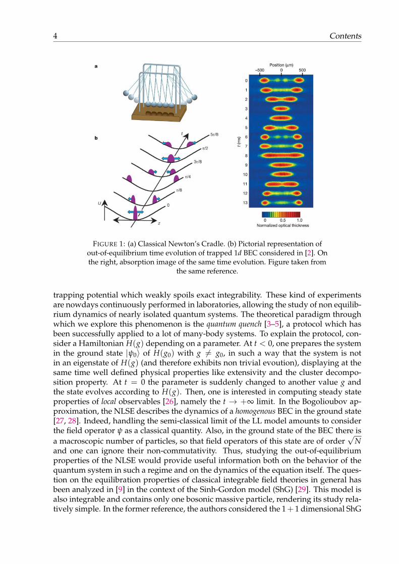


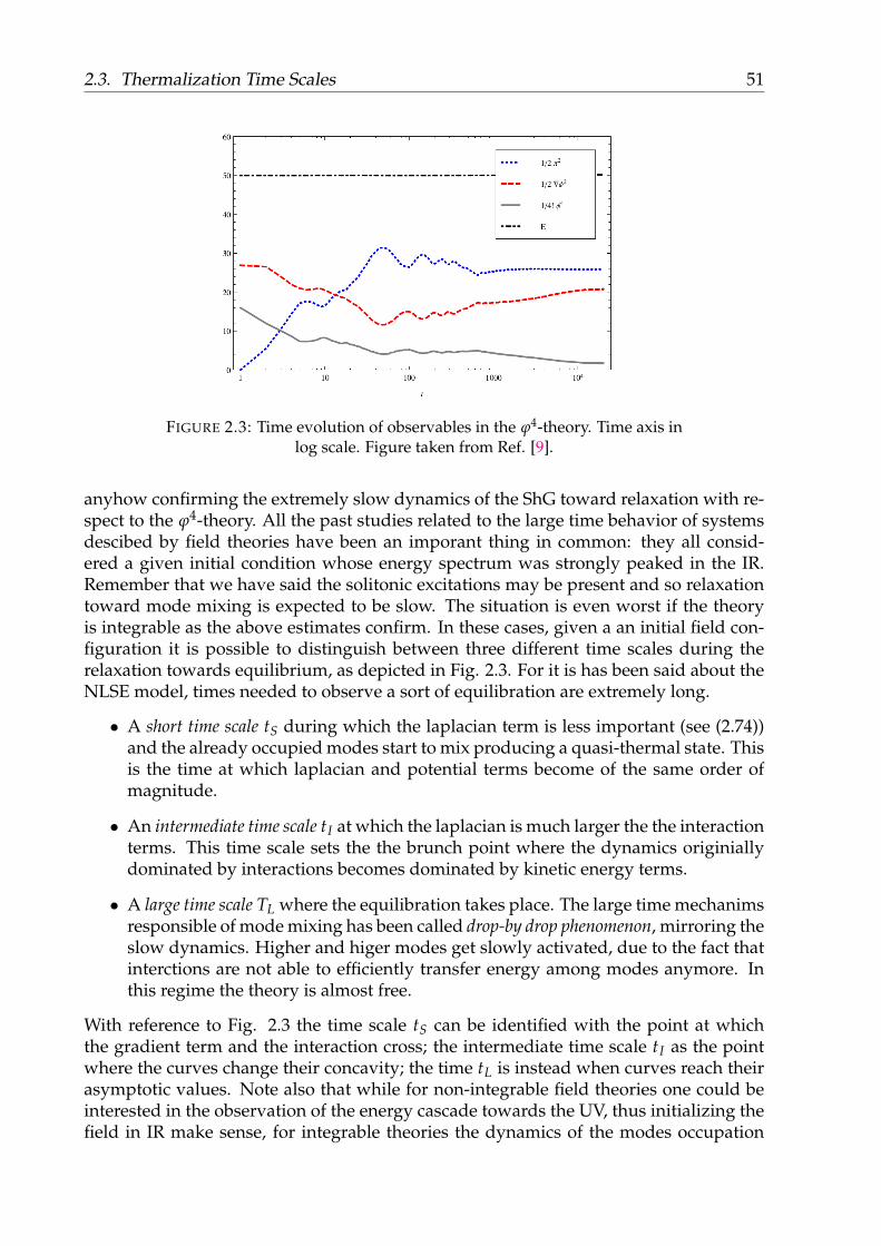


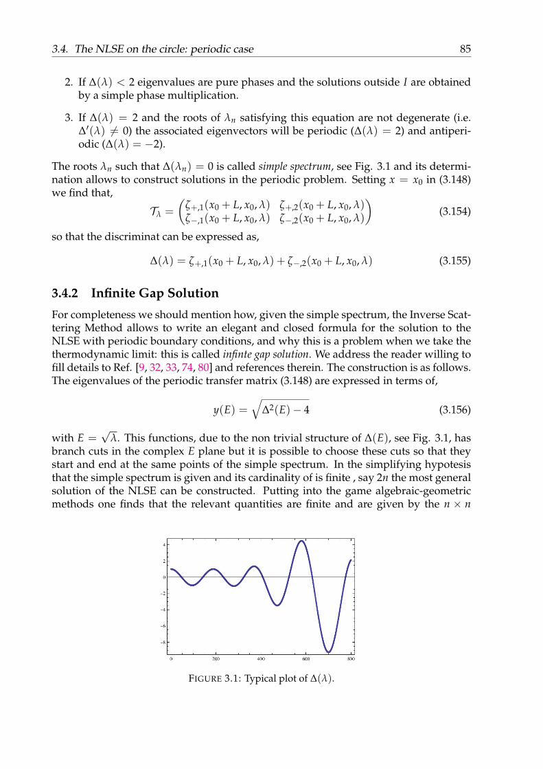


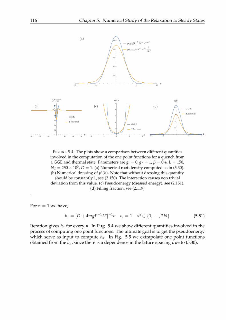

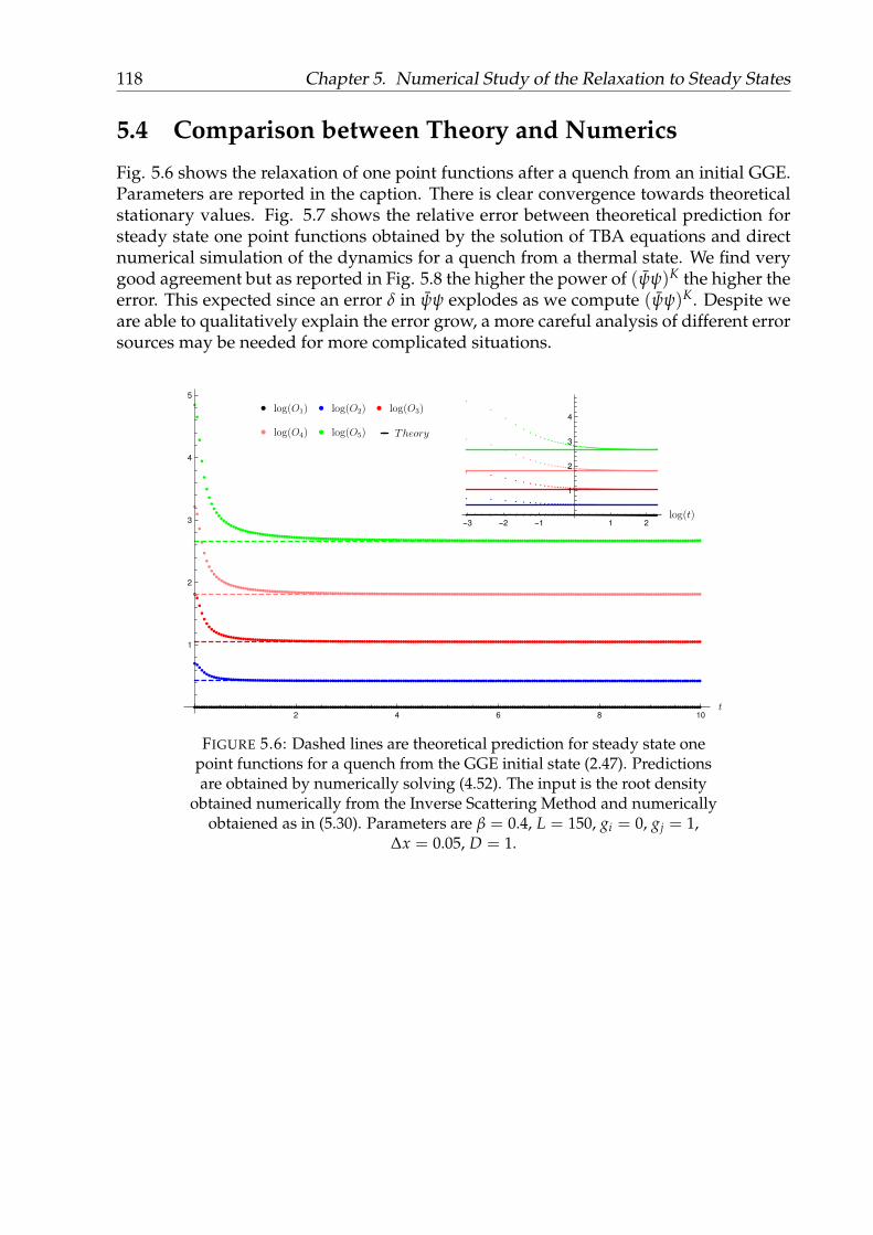
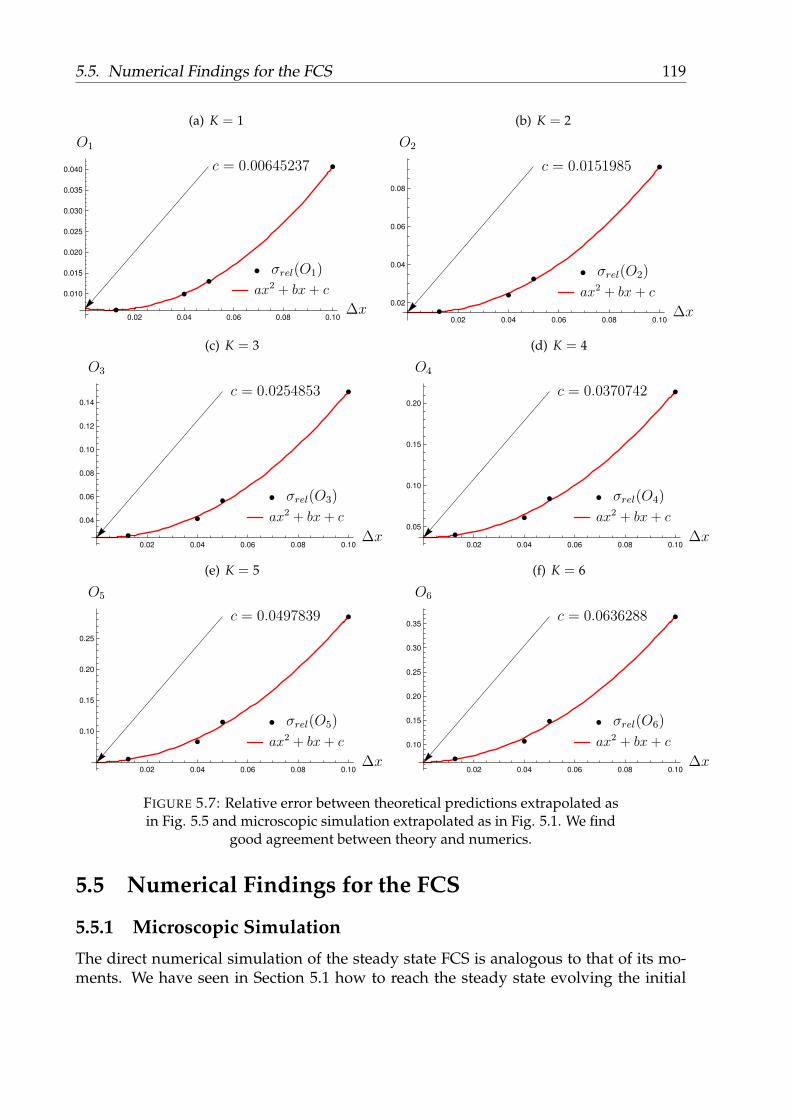


![On an integrable discretisation of the Lotka-Volterra system · all conserved quantities of the integrable system. This problem prompts a concept called integrable discretization[1].](https://static.documents.pub/doc/80x56/5f0ea3b77e708231d4403581/on-an-integrable-discretisation-of-the-lotka-volterra-all-conserved-quantities-of.jpg)
