Exact real-time dynamics of quantum spin systems using the positive-P representation This article has been downloaded from IOPscience. Please scroll down to see the full text article. 2011 J. Phys. A: Math. Theor. 44 065305 (http://iopscience.iop.org/1751-8121/44/6/065305) Download details: IP Address: 130.113.111.210 The article was downloaded on 15/07/2011 at 16:43 Please note that terms and conditions apply. View the table of contents for this issue, or go to the journal homepage for more Home Search Collections Journals About Contact us My IOPscience
Transcript
Exact real-time dynamics of quantum spin systems using the positive-P representation
This article has been downloaded from IOPscience. Please scroll down to see the full text article.
2011 J. Phys. A: Math. Theor. 44 065305
(http://iopscience.iop.org/1751-8121/44/6/065305)
Download details:
IP Address: 130.113.111.210
The article was downloaded on 15/07/2011 at 16:43
Please note that terms and conditions apply.
View the table of contents for this issue, or go to the journal homepage for more
Home Search Collections Journals About Contact us My IOPscience
Received 27 September 2010, in final form 17 December 2010Published 17 January 2011Online at stacks.iop.org/JPhysA/44/065305
AbstractWe discuss a scheme for simulating the real-time quantum quench dynamics ofinteracting quantum spin systems within the positive-P formalism. As modelsystems we study the transverse field Ising model as well as the Heisenbergmodel undergoing a quench away from the classical ferromagnetic ordered stateand the antiferromagnetic Neel state, depending on the sign of the Heisenbergexchange interaction. The connection to the positive-P formalism as it isused in quantum optics is established by mapping the spin operators on toSchwinger bosons. In doing so, the dynamics of the interacting quantum spinsystem is mapped onto a set of Ito stochastic differential equations the numberof which scales linearly with the number of spins, N, compared to an exactsolution through diagonalization that, in the case of the Heisenberg model,would require matrices exponentially large in N. This mapping is exact and canbe extended to higher dimensional interacting systems as well as to systemswith an explicit coupling to the environment.
PACS numbers: 05.10.Gg, 75.10.Pq, 75.10.Jm
(Some figures in this article are in colour only in the electronic version)
1. Introduction
The real-time quantum dynamics following a quench [1–15] is a problem of considerablecurrent interest. Here, our focus is on methods applicable to this problem that are in principleexact (up to controllable errors) and we leave approximate methods aside. Unfortunately,standard quantum Monte Carlo techniques yield results in the imaginary time domain andrequire an explicit analytic continuation to access real times, a notoriously difficult procedure.For lattice-based models it is possible to perform exact diagonalization but for an N sitequantum spin system the size of the Hilbert space is exponential in N, severely limiting
J. Phys. A: Math. Theor. 44 (2011) 065305 R Ng and E S Sørensen
the applicability of this method. In recent years, methods rooted in the density matrixrenormalization group (DMRG) such as TEBD [16] and t-DMRG [17] have been developed tostudy real-time dynamics of one-dimensional systems. Most recently the infinite size TEBD(iTEBD) has been tuned to yield results for the time dependence of the transverse field Isingmodel (TFIM) out to relatively large times of order tJ/h ∼ 6–10 [18] as well as in the XXZand related spin chain models tJ/h ∼ 20 [5, 9] and often times scales of order tJ/h ∼ 100 canbe accessed [19]. How well such methods will perform in higher dimensions or in the presenceof a coupling to the environment is presently a point of intense research and very promisingprogress has been made [20–23]. Here we investigate an alternative approach for studyingthe dynamics of interacting quantum spin systems using quantum phase space methods, inparticular, the positive-P representation (PPR) [24] of the density operator. As model systemswe have studied the one-dimensional TFIM as well as the Heisenberg model. This approachis quite general and can be extended to higher dimensional interacting quantum spin systemsand to open systems with an explicit coupling to the environment.
In general, quantum phase space methods map the dynamics of bosonic operators ontothe stochastic evolution of complex phase space variables [24]. Using the PPR, we can easilycalculate the expectation values of any normal-ordered products of creation and annihilationoperators by calculating the stochastic averages of their equivalent representation in termsof phase-space variables. This is carried out in two steps; first we use Schwinger bosons toreplace the Heisenberg spin operators, then employ the PPR. The PPR converts the masterequation into a Fokker–Planck equation (FPE) which can then be mapped onto a set of coupled,complex Ito stochastic differential equations (SDEs). The number of SDEs to simulate scaleslinearly with the number of spins in the system, N, in contrast to an exact diagonalizationapproach.
To illustrate the feasibility of this approach we study the dynamics of the TFIM as wellas the isotropic ferromagnetic (FM) Heisenberg model subject to a quantum quench at T = 0.The different models are related through the anisotropy parameter, �/J . The spin chains areprepared in the FM state at t = 0 whenever we assume a FM Heisenberg model, and evolvedby including the transverse magnetic field term at t � 0. We calculate the time evolution of theexpectation values of the spin operators: [Sx] , [Sy] [Sz], which is an average of the individualcomponents over the entire lattice. The averaging is allowed because of the translationalsymmetry of the system. In addition, we also calculate the results of Sz nearest-neighborcorrelation functions:
[Sz
i Szi+1
]for the TFIM. In order to verify the validity of our results,
we in all cases compare them with results from exact diagonalization obtaining the excellentagreement.
In a bid to fully take advantage of the PPR, we also attempt to explore finite size effectsby simulating lattice sizes of up to 100 spins for the FM isotropic model and 10 spins for theantiferromagnetic (AFM) anisotropic model. Finite size effects are more noticeable in theAFM Hamiltonian, and for the latter the natural choice for an initial state is the classical Neelstate.
Since the PPR is well established in quantum optics, we will relegate the details of theformalism to appendix A. Readers who are already familiar with the PPR may continue tosection 2 where Schwinger bosons are employed to map the spin operators onto bosonicoperators. The resulting SDEs are derived in this section with more explicit details laid out inappendic C. In section 3, the results of the TFIM (�/J = 0.0) and the isotropic (�/J = 1.0)
Heisenberg model are compared with exact diagonalization calculations. We also carry outa brief discussion on the possibility of extending simulation life times by potentially usingthe gauge-P representation [25] instead. In section 3.1, we present our results for finite-sizeeffects in both the anisotropic AFM and the isotropic FM Hamiltonian and discuss our findings.
2
J. Phys. A: Math. Theor. 44 (2011) 065305 R Ng and E S Sørensen
Results and a short discussion on the correlation functions can be found in section 3.2. Theconclusion is presented in section 4.
2. Using Schwinger bosons to derive SDEs
The PPR is based on bosonic coherent states and is only directly applicable to Hamiltonianswritten in terms of bosonic annihilation and creation operators. In order to apply it tothe Heisenberg model or any spin Hamiltonian, we therefore need to rewrite the spinoperators in terms of bosonic operators. A convenient way of doing this is by employingthe Schwinger boson representation [26, 27] and we will demonstrate how it can be appliedto the Heisenberg model. A similar approach, based on Schwinger bosons, was previouslyapplied to the study of spontaneous emission non-interacting two-level atoms [28] in quantumoptics.
The Heisenberg Hamiltonian with FM (J > 0) or AFM interaction (J < 0) subject to aquench in the x-direction at t � 0 is given by
H = −J∑〈i,j〉
Si · Sj − h(t)∑
i
Sxi , h(t) =
{h, t � 00, t < 0
(1)
and can be written in terms of the usual raising and lowering operators, S± = Sx ± iSy. If weallow anisotropy in the transverse direction1, then the Hamiltonian takes the following form:
HHeis = −∑〈i,j〉
[J Sz
i Szj + �
1
2
(S+
i S−j + S−
i S+j
)]− 1
2h(t)
∑i
[S+
i + S−i
](2)
where 〈i, j 〉 indicates nearest-neighbor pairs and �/J is a measure of anisotropy. The twomodels which we first examined were the (i) TFIM (�/J = 0):
HTFIM = −∑〈i,j〉
[J Sz
i Szj
]− 1
2h(t)
∑i
[S+
i + S−i
](3)
and the (ii) isotropic Heisenberg model (see equation (2)) with an anisotropy of �/J = 1.0.The Schwinger boson representation of spins (setting h = 1) is given by
S+ → ba†, S− → b†a, Sz → 12 (a†a − b†b). (4)
where a and b represent two types of bosons and the following commutation relations:[S+, S−] → [
a†b, b†a] = a†a − b†b → 2Sz,[
S+, Sz] →
[a†b,
1
2(a†a − b†b)
]= −a†b → −S+, (5)
[S−, Sz
] →[b†a,
1
2(a†a − b†b)
]= b†a → S−
demonstrate that the commutation relations of the spin operators are indeed preserved. Thisis a necessary requirement for a successful mapping. With the Schwinger representation, thetwo states of a spin-1/2 particle are now described by either an a-boson or a b-boson per site.A spin-up state: |↑〉 is the same as having a single a-boson whereas a spin down-state: |↓〉 isthe same as having a single b-boson. We can therefore replace the spin operators in equations(2) and (3) with the bosonic mapping in equation (4) without altering the physics.
1 The transverse direction is relative to the quantization axis which we have taken to be the z-axis.
3
J. Phys. A: Math. Theor. 44 (2011) 065305 R Ng and E S Sørensen
As the PPR is well established2, we will relegate a brief review of the formalism toappendix A. Additional technical details pertaining to the specific examples in this paper canbe found in appendix C. For brevity we will present the derivations for only the TFIM (seeequation (3)) where �/J = 0.
Using equation (4), the equivalent bosonic Hamiltonian for the TFIM is given by
H = −J
4
∑〈i,j〉
(a†i ai a
†j aj − a
†i ai b
†j bj − b
†i bi a
†j aj + b
†i bi b
†j bj
)−(
h(t)∑
i
a†i bi + b
†i ai
). (6)
Now if we take our system to be closed, its dynamics can be captured via the masterequation for the density operator, i.e.
d
dtρ = − i
h
[H , ρ
], (7)
which allows us to use a generalized prescription of the PPR. In principle, it is also possibleto calculate open system dynamics by including a Liouvillan term in equation (7): L[ρ],3 andso this approach is by no means limited to closed system.
To proceed, we first write our density operator in terms of a direct product of projectionoperators for each site, i.e.
We can then use the usual correspondence relations (see equation (A.3)) to obtain an FPE (seeequation (A.4)) for the PPR distribution function: P(�α, �α+, �β, �β+). A particular factorizationof the diffusion matrix results in a noise matrix which gives us a set of Ito SDEs for 4N of ourphase space variables, i.e.
dαi ={
iJ
4hαi
[(nα
i+1 − nβ
i+1
)+(nα
i−1 − nβ
i−1
)]+
ih(t)
2hβi
}dt
+1
2
√iJ
2h
[−√αiαi+1
(dWα
2i + i dWα2i+1
)− √αiαi−1
(dWα
2i−2 − i dWα2i−1
)]+
i
2
√iJ
2h
[−√
αiβi−1(dW
αβ
2i−2 + i dWαβ
2i−1
)−√
αiβi+1(dW
βα
2i − i dWβα
2i+1
)](10)
dβi ={
iJ
4hβi
[(n
β
i+1 − nαi+1) + (n
β
i−1 − nαi−1)
]+
ih(t)
2hαi
}dt
+1
2
√iJ
2h
[−√
βiβi+1(dW
β
2i + i dWβ
2i+1
)−√
βiβi−1(dW
β
2i−2 − i dWβ
2i−1
)]
+i
2
√iJ
2h
[−√
αi+1βi
(dW
αβ
2i − i dWαβ
2i+1
)−√
αi−1βi
(dW
βα
2i−2 + i dWβα
2i−1
)](11)
2 See [28–33] for successful applications of the PPR.3 The Liouvillian term models the effect of the environment on the system.
4
J. Phys. A: Math. Theor. 44 (2011) 065305 R Ng and E S Sørensen
dα+i =
{iJ
4hα+
i
[(n
β
i+1 − nαi+1
)+(n
β
i−1 − nαi−1
)]− ih(t)
2hβ+
i
}dt
+i
2
√iJ
2h
[−√
α+i α+
i+1
(dWα+
2i + i dWα+
2i+1
)−√
α+i α+
i−1
(dWα+
2i−2 − i dWα+
2i−1
)]+
1
2
√iJ
2h
[−√
α+i β+
i−1
(dW
α+β+
2i−2 + i dWα+β+
2i−1
)−√
α+i β+
i+1
(dW
β+α+
2i − i dWβ+α+
2i+1
)](12)
dβ+i =
{iJ
4hβ+
i
[(nα
i+1 − nβ
i+1
)+(nα
i−1 − nβ
i−1
)]− ih(t)
2hα+
i
}dt
+i
2
√iJ
2h
[−√
β+i β+
i+1
(dW
β+
2i + i dWβ+
2i+1
)−√
β+i β+
i−1
(dW
β+
2i−2 − i dWβ+
2i−1
)]+
1
2
√iJ
2h
[−√
α+i+1β
+i
(dW
α+β+
2i − i dWα+β+
2i+1
)−√
α+i−1β
+i
(dW
β+α+
2i−2 + i dWβ+α+
2i−1
)], (13)
where i = 0 . . . N − 1 labels the vector components and we have defined nαi = α+
i αi andn
β
i = β+i βi , which are complex phase space functions representing the number of a and
b-bosons (per site i), respectively. With this particular choice of noise matrix, we haveintroduced eight 2N × 1 Wiener increment vectors with the usual statistical propertiesthat 〈dWx
i dWy
j 〉 = dtδxyδij and 〈dWxi 〉 = 0, where i = 0 . . . N − 1 and x, y =
α, α+, β, β+, βα, αβ, β+α+, α+β+ labels each Wiener increment vector. We would like topoint out that the subscript labels of the Wiener increment vector are not unique and thelabeling scheme4 was chosen simply for convenience (see appendix C).
2.1. Inclusion of anisotropy
Had we begun with the full anisotropic Hamiltonian in equation (2) instead and carried outthe same steps as in section 2, it would have been shown that anisotropy is included by addingthe following expressions into the drift terms of equations (10)–(13):
dαi ∼ +i�
2hβi(mi−1 + mi+1) dt (14)
dβi ∼ +i�
2hαi(m
+i−1 + m+
i+1) dt (15)
dα+i ∼ − i�
2hβ+
i (m+i−1 + m+
i+1) dt (16)
dβ+i ∼ − i�
2hα+
i (m+i−1 + m+
i+1) dt (17)
where the following shorthand mi = αiβ+i , m+
i = α+i βi was used. For the stochastic terms,
however, only the mixed derivative diffusion terms (i.e. those containing αβ and α+β+) aremodified in the following way:
dαi ∼ +i
2
√i
2h
[−√
Jαiβi−1 − 2�βiαi−1(. . . . . .) −√
Jαiβi+1 − 2�αi+1βi(. . . . . .)]
(18)
4 Note that with the inclusion of periodic boundary conditions: α−1 → αN−1 and αN → α0. However, since thereare 2N × 1 Wiener increments, then it is periodic in 2N instead. For example dWx
−1 = dWx2N−1 and dWx
2N = 0.
5
J. Phys. A: Math. Theor. 44 (2011) 065305 R Ng and E S Sørensen
dβi ∼ +i
2
√i
2h
[−√
Jβiαi+1 − 2�βi+1αi(. . . . . .) −√
Jβiαi−1 − 2�αiβi−1(. . . . . .)]
(19)
dα+i ∼ +
i
2
√i
2h
[−√
Jβ+i−1α
+i − 2�β+
i α+i−1(. . . . . .) −
√Jβ+
i+1α+i − 2�α+
i+1β+i (. . . . . .)
](20)
dβ+i ∼ +
i
2
√i
2h
[−√
Jβ+i α+
i−1 − 2�β+i−1α
+i (. . . . . .) −
√Jβ+
i α+i+1 − 2�α+
i β+i+1(. . . . . .)
](21)
where the terms in (. . . . . .) represent the same Wiener increment combinations as in equations(10)–(13). The Ito SDEs we have derived are able to describe other types of spins modelssuch as the XY model and the XYZ model (to name a few), just by adjusting or includinga few parameters. For the last two cases, we would have to take a trivial generalization inthe derivations by introducing two different anisotropy terms in equation (2). An informativereview article on the the quantum quench dynamics of other variants of the HeisenbergHamiltonian using other numerical methods can be found in [9].
3. Results and discussion
To test our formalism, we first simulated the FM (J > 0) spin Hamiltonian for the TFIM(�/J = 0) and the isotropic Heisenberg Hamiltonian (�/J = 1.0) in equation (2) forhigh (h/J = 10) and low (h/J = 0.5) field values. This was compared to results fromexact diagonalization calculations using a small system with N = 4 spins. The Stratanovichversion of the SDES5 in equations (10)–(13) were simulated using a semi-implicit Stratanovichalgorithm as they are known to exhibit superior convergence properties [34]. To track thedynamics of the system, we calculated the expectation values of all three spin components ateach site i: 〈Sx
i 〉, 〈Sy
i 〉, 〈Szi 〉. Using the translation symmetry of the system, we further averaged
them over the entire lattice to obtain an average expectation value of the spin components persite: [Sx] , [Sy] , [Sz]. These expectation values were calculated using the stochastic averagesof their respective phase space functions, i.e.
[Sx] =
N−1∑i=0
⟨1
2
(a†i bi + b
†i ai
)⟩ =N−1∑i=0
⟨⟨1
2
(α+
i βi + β+i αi
)⟩⟩, (22)
[Sy] =
N−1∑i=0
⟨1
2i
(a†i bi − b
†i ai
)⟩ =N−1∑i=0
⟨⟨1
2i
(α+
i βi − β+i αi
)⟩⟩, (23)
[Sz] =
N−1∑i=0
⟨1
2
(a†i ai − b
†i bi
)⟩ =N−1∑i=0
⟨⟨1
2
(α+
i αi − β+i βi
)⟩⟩, (24)
where 〈〈·〉〉 denotes a stochastic average.The initial state of the system was taken to be the classical FM state: | ↑↑ . . . ↑〉 and the
dynamics were observed for t � 0 during which a transverse field is turned on. The resultsfor the TFIM are shown in figures 1 and 2 for different field strengths while the results forthe isotropic (�/J = 1.0) model are shown in figures 3 and 4. Both models show a goodagreement with exact diagonalization calculations.
5 The Stratanovich correction terms worked out to be zero and hence the Stratanovich form of the SDEs fromequations (10)–(13) have the exact same form as the derived Ito SDEs.
6
J. Phys. A: Math. Theor. 44 (2011) 065305 R Ng and E S Sørensen
0
0.01
0.02
0.03
0.04
0.05
0 0.1 0.2 0.3 0.4 0.5 0.6
[Sx ]
tJ/−h
0
0.04
0.08
0.12
[Sy ]
0.4
0.42
0.44
0.46
0.48
0.5
[Sz ]
Figure 1. TFIM following a transverse quench. From top to bottom: plots of [Sx ] , [Sy ] , [Sz]versus tJ/h, respectively. The stochastic averages, 〈〈·〉〉 are given by red solid lines whileexact diagonalization results are represented by green dashed lines. Simulation parameters:N = 4, ntraj = 106, dt = 0.001, h/J = 0.5,�/J = 0.0. The agreement remains good untilapproximately tJ/h = 0.6.
0
0.01
0.02
0 0.1 0.2 0.3 0.4 0.5 0.6
[Sx ]
tJ/−h
-0.5
-0.3
-0.1
0.1
0.3
0.5
[Sy ]
-0.5
-0.3
-0.1
0.1
0.3
0.5
[Sz ]
Figure 2. TFIM following a transverse quench. From top to bottom: plots of [Sx ] , [Sy ] , [Sz]versus tJ/h, respectively. The stochastic averages, 〈〈·〉〉 are given by red solid lines whileexact diagonalization results are represented by the green dashed lines. Simulation parameters:N = 4, ntraj = 2 × 10⁵, dt = 0.001, h/J = 10.0,�/J = 0.0. Agreement remains good untilapproximately tJ/h = 0.65.
7
J. Phys. A: Math. Theor. 44 (2011) 065305 R Ng and E S Sørensen
-0.0001
-5e-05
0
5e-05
0 0.1 0.2 0.3 0.4
[Sx ]
tJ/−h
0
0.04
0.08
[Sy ]
0.485
0.49
0.495
0.5
[Sz ]
Figure 3. Isotropic Heisenberg model following a transverse quench. From top to bottom: plotsof [Sx ] , [Sy ] , [Sz] versus tJ/h, respectively. The stochastic averages, 〈〈·〉〉 are given by redsolid lines while exact diagonalization results are represented by green dashed lines. Simulationparameters: N = 4, ntraj = 106, dt = 0.001, h/J = 0.5,�/J = 1.0. The agreement remainsgood and both results are nearly indistinguishable. The simulations diverge at approximatelytJ/h = 0.45.
The only drawback of the PPR is that the simulations are usually valid only for relativelyshort lifetimes (roughly tJ/h ∼ 0.45–0.65 for the models examined) before sampling errorscaused by diverging trajectories take over. In figure 1 for example, the onset of the effects ofdiverging trajectories can be seen at around tJ/h ∼ 0.58 where a deviation of the SDE resultsand exact calculations begin to appear. However, for the time scales where the simulationsremain finite, it does yield good results.
One should not be alarmed as this is a common problem associated with using the PPRand can be attributed to the nature of the SDEs derived and not due to a non-convergingnumerical algorithm [35–37]. In fact, Deuar [38] examined this issue when applying the PPRto the exact dynamics of many-body systems. If we abide by Deuar’s findings strictly,we see that there are no drift and noise divergences present in the SDEs in equations(10)–(13). However, we suspect drift terms of the form ∼ iXi
[( ∓ nαi+1 ± n
β
i+1
)+(nα
i−1 ±n
β
i−1
)], where Xi = αi, α
+i , β, β+ can be problematic. This is because if we take into
consideration the translational symmetry of the system, then we can approximately saythat
iXi
[(∓ nαi+1 ± n
β
i+1
)+(∓ nα
i−1 ± nβ
i−1
)] ≈ 2iXi
(∓ nαi ± n
β
i
), (25)
which now clearly exhibits offending terms [38] that cause trajectories to escape to infinity,since dXi ∼ X2
i [· · ·] dt + · · ·.The gauge-P representation [25, 37–40] was developed to specifically deal with such drift
instabilities. In the gauge-P representation, arbitrary gauge functions, {gk} can be introducedinto the SDEs whose effect is a modification of the deterministic evolution. This can be doneat the expense of introducing another stochastic variable (�), in �, which manifests itself as
8
J. Phys. A: Math. Theor. 44 (2011) 065305 R Ng and E S Sørensen
-0.0006
-0.0004
-0.0002
0
0 0.1 0.2 0.3 0.4
[Sx ]
tJ/−h
-0.5
-0.3
-0.1
0.1
0.3[S
y ]-0.5
-0.3
-0.1
0.1
0.3
0.5
[Sz ]
Figure 4. Isotropic Heisenberg model following a transverse quench. From top to bottom: plotsof [Sx ] , [Sy ] , [Sz] versus tJ/h, respectively. The stochastic averages, 〈〈·〉〉 are given by redsolid lines while exact diagonalization results are represented by green dashed lines. Simulationparameters: N = 4, ntraj = 105, dt = 0.001, h/J = 10.0,�/J = 1.0. The agreement remainsgood and both results are nearly indistinguishable. The simulations diverge at approximatelytJ/h = 0.45.
a weight term when calculating stochastic averages. To be more specific using the gauge-Prepresentation [25], the Ito SDEs are altered such that
dαi = (A+
i − gkBjk
)dWk (26)
d� = �(V dt + gkdWk), (27)
where summation over k is implied and V is the constant term that may appear after substitutingthe correspondence relations into an equation of motion for ρ.
The gauge-P representation has been very successful in simulating the dynamics of many-mode Bose gases [41–43] partly because such systems result in neat diagonal noise matricesthat are easier to handle as seen in equation (26). However, it is evidently not as straightforwardto apply it in our case as we have a much more complicated non-diagonal noise matrix. Thetrue complication arises when we attempt to calculate Stratonovich correction terms as it isthe Stratanovich version of the SDEs that are simulated. We believe that the application of thegauge-P is possible in principle but requires a bit more thought for Heisenberg systems whenusing the Schwinger boson approach.
3.1. Finite size effects
The main advantage of the PPR is the linear scaling with the number of spins, N, as comparedto the exponentially large matrices needed for an exact solution. We first demonstrate thecapabilities of the PPR at simulating large system sizes by showing results for the FMisotropic Heisenberg case at a field value of h/J = 10, prepared in the initial FM state
9
J. Phys. A: Math. Theor. 44 (2011) 065305 R Ng and E S Sørensen
-0.0008
-0.0004
0
0.0004
0 0.1 0.2 0.3 0.4
[Sx ]
tJ/−h
-0.5
-0.3
-0.1
0.1
0.3[S
y ]-0.5
-0.3
-0.1
0.1
0.3
0.5
[Sz ]
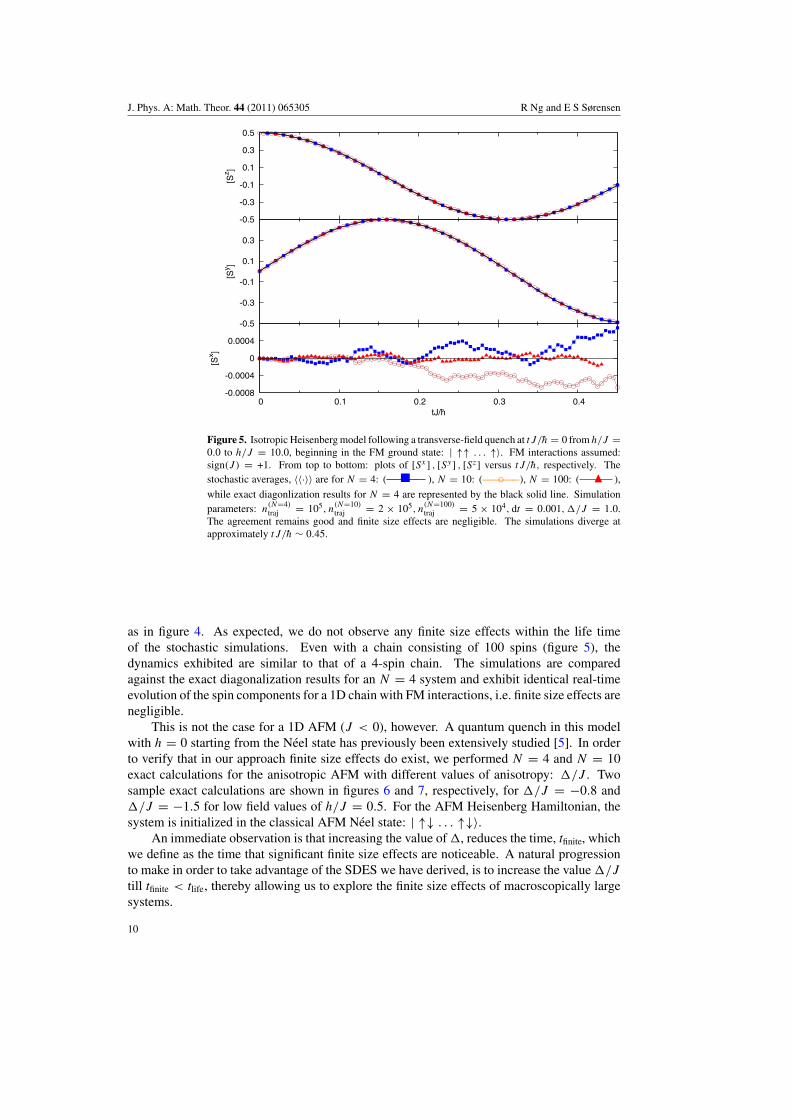
Figure 5. Isotropic Heisenberg model following a transverse-field quench at tJ/h = 0 from h/J =0.0 to h/J = 10.0, beginning in the FM ground state: | ↑↑ . . . ↑〉. FM interactions assumed:sign(J ) = +1. From top to bottom: plots of [Sx ] , [Sy ] , [Sz] versus tJ/h, respectively. Thestochastic averages, 〈〈·〉〉 are for N = 4: ( ), N = 10: ( ◦ ), N = 100: ( ),
while exact diagonlization results for N = 4 are represented by the black solid line. Simulationparameters: n
(N=4)traj = 105, n
(N=10)traj = 2 × 10⁵, n
(N=100)traj = 5 × 10⁴, dt = 0.001,�/J = 1.0.
The agreement remains good and finite size effects are negligible. The simulations diverge atapproximately tJ/h ∼ 0.45.
as in figure 4. As expected, we do not observe any finite size effects within the life timeof the stochastic simulations. Even with a chain consisting of 100 spins (figure 5), thedynamics exhibited are similar to that of a 4-spin chain. The simulations are comparedagainst the exact diagonalization results for an N = 4 system and exhibit identical real-timeevolution of the spin components for a 1D chain with FM interactions, i.e. finite size effects arenegligible.
This is not the case for a 1D AFM (J < 0), however. A quantum quench in this modelwith h = 0 starting from the Neel state has previously been extensively studied [5]. In orderto verify that in our approach finite size effects do exist, we performed N = 4 and N = 10exact calculations for the anisotropic AFM with different values of anisotropy: �/J . Twosample exact calculations are shown in figures 6 and 7, respectively, for �/J = −0.8 and�/J = −1.5 for low field values of h/J = 0.5. For the AFM Heisenberg Hamiltonian, thesystem is initialized in the classical AFM Neel state: | ↑↓ . . . ↑↓〉.
An immediate observation is that increasing the value of �, reduces the time, tfinite, whichwe define as the time that significant finite size effects are noticeable. A natural progressionto make in order to take advantage of the SDES we have derived, is to increase the value �/J
till tfinite < tlife, thereby allowing us to explore the finite size effects of macroscopically largesystems.
10
J. Phys. A: Math. Theor. 44 (2011) 065305 R Ng and E S Sørensen
0
0.01
0.02
0.03
0 0.5 1 1.5 2
[Sx ]
tJ/−h
-0.15
-0.1
-0.05
0
0.05
0.1
[Sy ]
-0.1
0
0.1
0.2
0.3
0.4
0.5
[Sz ]
Figure 6. Anisotropic Heisenberg model following a transverse-field quench at tJ/h = 0 fromh/J = 0.0 to h/J = 10.0, beginning in the AFM Neel state: | ↑↓ . . . ↑↓〉. AFM interactionsassumed: sign(J ) = −1. From top to bottom: plots of [Sx ] , [Sy ] , [Sz] versus tJ/h, respectively.The exact calculations for the N = 4 (solid black lines) and N = 10 (dashed red lines) arecompared. We observe tfiniteJ/h ∼0.8 for �/J ∼ −0.8.
-0.12
-0.08
-0.04
0
0 0.5 1 1.5 2
[Sx ]
tJ/−h
-0.25
-0.2
-0.15
-0.1
-0.05
0
0.05
[Sy ]
-0.5
-0.3
-0.1
0.1
0.3
0.5
[Sz ]
Figure 7. Anisotropic Heisenberg model following a transverse-field quench at tJ/h = 0 fromh/J = 0.0 to h/J = 10.0, beginning in the AFM Neel state: | ↑↓ . . . ↑↓〉. AFM interactionsassumed: sign(J ) = −1. From top to bottom: plots of [Sx ] , [Sy ] , [Sz] versus tJ/h, respectively.The exact calculations for the N = 4 (solid black lines) and N = 10 (dashed red lines) arecompared. We observe tfiniteJ/h ∼ 0.5 for a given anisotropy of �/J ∼ −1.5.
11
J. Phys. A: Math. Theor. 44 (2011) 065305 R Ng and E S Sørensen
0
0.004
0.008
0.012
0 0.25 0.5 0.75 1
[Sx ]
tJ/−h
-0.5
-0.3
-0.1
0.1
0.3
[Sy ]
-0.5
-0.3
-0.1
0.1
0.3
[Sz ]
Figure 8. Anisotropic Heisenberg model following a transverse-field quench at tJ/h = 0 fromh/J = 0.0 to h/J = 10.0, beginning in the AFM ground state: | ↑↓ . . . ↑↓〉. AFM interactionsassumed: sign(J ) = −1. From top to bottom: plots of [Sx ] , [Sy ] , [Sz] versus tJ/h, respectively.The stochastic averages, 〈〈·〉〉 are for N = 4: ( ) and N = 10: ( ◦ ), while exact
diagonalization results are for N = 4: (black solid lines) and N = 10: ( ). Simulation
good and finite size effects are unnoticeable up to tJh = 1. The SDEs diverge at tlifeJ/h ∼ 0.48.
We observe finite size effects through the same observables as in equations (22) to(24). However for the initial Neel state, it is more meaningful to take into consideration thealternating sign of spins when calculating the averaged spin components6, i.e.
[Sx] =
N−1∑i=0
⟨1
2
(a†i bi + b
†i ai
)⟩ =N−1∑i=0
⟨⟨1
2
(α+
i βi + β+i αi
)⟩⟩, (28)
[Sy] =
N−1∑i=0
⟨1
2i(−1)i
(a†i bi − b
†i ai
)⟩ =N−1∑i=0
(−1)i⟨⟨
1
2i
(α+
i βi − β+i αi
)⟩⟩, (29)
and
[Sz] =
N−1∑i=0
⟨1
2(−1)i
(a†i ai − b
†i bi
)⟩ =N−1∑i=0
(−1)i⟨⟨
1
2
(α+
i αi − β+i βi
)⟩⟩. (30)
Increasing �/J however has the adverse effect of decreasing tlife significantly. Thus, while itis possible to simulate macroscopically large system sizes, we find that the SDE simulationsdiverge much sooner than tfinite. Figure 8 (�/J = −0.5, h/J = 10.0) reinforces our claimthat tfinite decreases with �/J as no finite size effects are observed up to tJ/h = 1, in sharpcomparison to figure 6 (�/J = −0.8) and figure 7 (�/J = −1.5), albeit for h/J = 0.5.
6 Note that there exists an exception. There is no need to account for a sign change for the observable: [Sx ].
12
J. Phys. A: Math. Theor. 44 (2011) 065305 R Ng and E S Sørensen
0 0.001 0.002 0.003 0.004 0.005
0 0.1 0.2 0.3 0.4
[Sx ]
tJ/−h
0
0.02
0.04
0.06
0.08[S
y ] 0.44
0.46
0.48
0.5
[Sz ]
Figure 9. Anisotropic Heisenberg model following a transverse-field quench at tJ/h = 0 fromh/J = 0.0 to h/J = 0.5, beginning in the AFM ground state: | ↑↓ . . . ↑↓〉. AFM interactionsassumed: sign(J ) = −1. From top to bottom: plots of [Sx ] , [Sy ] , [Sz] versus tJ/h, respectively.The stochastic averages, 〈〈·〉〉 are for N = 4: ( ◦ ) and N = 10: ( ∗ ), while exact
diagonalization results are for N = 4: (black solid lines) and N = 10: ( ). Simulation
Our last effort to observe finite size effects was to increase �/J to −0.8 with hopes thattlife > tfinite. As seen in figure 9, our simulations do not survive beyond tfinite. Since tfinite
depends on the anisotropy �/J , increasing the system size while possible will result in tlife ofthe same order. In general, we find that increasing �/J will decrease tlife as well as tfinite suchthat tlife < tfinite always holds true. This thwarts our efforts to examine finite size effects for theAFM case. Furthermore, we find that using an initial Neel state results in poor convergencefor the observable: [Sx] as seen in figure 8 (and even more so in figure 9) compared to aninitial FM ground state and it is likely that we have used an insufficient number of trajectoriesin our simulations. Nevertheless, we have demonstrated the applicability of the PPR to AFMsystems.
3.2. Nearest-neighbor correlation functions
Correlation functions are generally of greater interest seeing as they are experimentallyaccessible quantities. In order to demonstrate the applicability of the PPR in this respect,we calculate the nearest-neighbor spin correlation functions for the z-component, which isdefined as
[Sz
i Szi+1
] =N−1∑i=0
〈Szi S
zi+1〉
N= 1
4
N−1∑i=0
⟨⟨(nα
i − nβ
i
)(nα
i+1 − nβ
i+1
)⟩⟩N
, (31)
13
J. Phys. A: Math. Theor. 44 (2011) 065305 R Ng and E S Sørensen
0.23
0.235
0.24
0.245
0.25
[Sz i.S
z i+1]
0
0.05
0.1
0.15
0.2
0.25
0 0.1 0.2 0.3 0.4 0.5 0.6
[Sz i.S
z i+1]
tJ/−h
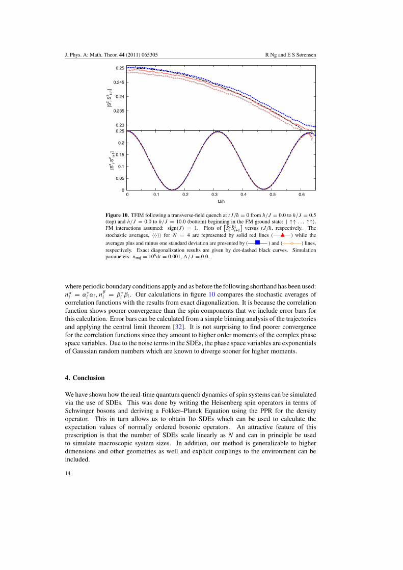
Figure 10. TFIM following a transverse-field quench at tJ/h = 0 from h/J = 0.0 to h/J = 0.5(top) and h/J = 0.0 to h/J = 10.0 (bottom) beginning in the FM ground state: | ↑↑ . . . ↑↑〉.FM interactions assumed: sign(J ) = 1. Plots of
[Sz
i Szi+1
]versus tJ/h, respectively. The
stochastic averages, 〈〈·〉〉 for N = 4 are represented by solid red lines ( ) while the
averages plus and minus one standard deviation are presented by ( ) and ( ◦ ) lines,respectively. Exact diagonalization results are given by dot-dashed black curves. Simulationparameters: ntraj = 106dt = 0.001,�/J = 0.0.
where periodic boundary conditions apply and as before the following shorthand has been used:nα
i = α+i αi, n
β
i = β+i βi . Our calculations in figure 10 compares the stochastic averages of
correlation functions with the results from exact diagonalization. It is because the correlationfunction shows poorer convergence than the spin components that we include error bars forthis calculation. Error bars can be calculated from a simple binning analysis of the trajectoriesand applying the central limit theorem [32]. It is not surprising to find poorer convergencefor the correlation functions since they amount to higher order moments of the complex phasespace variables. Due to the noise terms in the SDEs, the phase space variables are exponentialsof Gaussian random numbers which are known to diverge sooner for higher moments.
4. Conclusion
We have shown how the real-time quantum quench dynamics of spin systems can be simulatedvia the use of SDEs. This was done by writing the Heisenberg spin operators in terms ofSchwinger bosons and deriving a Fokker–Planck Equation using the PPR for the densityoperator. This in turn allows us to obtain Ito SDEs which can be used to calculate theexpectation values of normally ordered bosonic operators. An attractive feature of thisprescription is that the number of SDEs scale linearly as N and can in principle be usedto simulate macroscopic system sizes. In addition, our method is generalizable to higherdimensions and other geometries as well and explicit couplings to the environment can beincluded.
14
J. Phys. A: Math. Theor. 44 (2011) 065305 R Ng and E S Sørensen
The main drawback of the PPR, however, is its notoriously short life time which preventsus from obtaining useful results beyond a certain time: tlife. For the TFIM and the anisotropicHeisenberg model, we found a bare application of the PPR to have tlifeJ/h ∼ 0.45–0.65. Wesuspect that this is due to drift instability terms present in the SDEs that cause trajectories todiverge within this time scale.
We also attempted to explore finite size effects which were more significant for theanisotropic AFM Hamiltonian beginning in the classical Neel state. For the FM case, no finitesize effects were observed even for a lattice size of 100 spins within its lifetime. We find thatthe more negative the anisotropy parameter in the AFM Hamiltonian, the sooner finite sizeeffects are observed, i.e. tfinite decreases. However, this has the adverse effect of decreasingtlife such that tlife < tfinite for the simulations that we have carried out.
Finally, we would like to point that in cases where the underlying Hamiltonian hasconserved properties, such as the models addressed in this paper, then it could be advantageousto use projection methods instead [44, 45]. This ensures the use of a more efficient basis setwhich will lead to improved simulation performances. In particular, there exists the PPRapproach which uses the SU(n) spin coherent states [46] as a basis set instead.
An obvious future direction of our research involves applying the gauge-P representationin a bid to extend simulation life times and to examine the efficient of the other methodssuggested above. Also the study of systems in higher dimensions with and without couplingsto the environment would be of considerable interest.
Acknowledgments
This research has been made possible with the support of an NSERC research grant. Wewould also like to thank Piotr Deuar and Murray Olsen for helpful discussions.
Appendix A. The positive-P representation
In this section, we will review the PPR [24] that has been applied to both quantum optics[28–30] and exact many-body simulations of Bose gases [33, 47–49] successfully. The PPRis already well established and our aim for including this review is simply to provide aself-contained paper for readers who are not as familiar with it.
In short, the PPR is an expansion of the density operator in terms of an off-diagonalcoherent state basis:
ρ =∫
P(α, α+)�(α, α+) d2α d2α+ =∫
P(α, α+)|α〉〈α+∗|〈α+∗|α〉 d2α d2α+ (A.1)
where |α〉 = e− 12 |α|2 ∑∞
n=0αn
n! |n〉 is the standard bosonic coherent state [50] that are eigenstatesof the annihilation operator a. P(α, α+) plays the role of a distribution function in the phasespace spanned by {α, α+} and can be chosen such that it remains real and positive. In addition,due to the normalization factor in the denominator of equation (A.1) and using the fact thatTr[ρ] = 1, we see that∫
P(α, α+) d2α d2α+ = 1 (A.2)
i.e. the distribution is normalized over the entire complex phase space. Simply put, we caninterpret P(α, α+) as a probability distribution function for the variables α and α+, hence thename positive-P.
15
J. Phys. A: Math. Theor. 44 (2011) 065305 R Ng and E S Sørensen
A hallmark of the PPR is that the off-diagonal projection operators, �(α, α+) satisfies thefollowing correspondence relations:
a� = α�
a†� =(
α+ +∂
∂α
)� (A.3)
�a† = α+�
�a =(
α +∂
∂α+
)�,
which allows us to map complicated operator equations consisting of bosonic annihilationand creation operators onto differential equations of phase space variables α, α+. Thecorrespondence relation is typically used in an equation of motion for ρ, which after integrationby parts and ignoring of boundary terms allows us to obtain a FPE:
∂P (�x)
∂t={− ∂
∂xμAμ(�x) +
1
2
∂
∂xμ
∂
∂xνDμν(�x)
}P(�x), μ, ν = 0 . . . N − 1, (A.4)
where �x = {�α, �α+}, Aμ is called the drift vector and Dμν is called the diffusion matrix (whichis symmetric and positive semi-definite by definition). Due to the doubling of phase space,the diffusion matrix is guaranteed to be positive semi-definite [24]. This then allows one toconvert the FPE to a set of Ito SDEs proportional to the number of bosonic modes of thesystem, i.e.
where dWν is a vector of Wiener increments with Nw components and Bμν is a noise matrixthat must satisfy the factorization
D = BBT . (A.6)
This factorization is not unique and any noise matrix that satisfies equation (A.6) will producethe same stochastic averages in the limit of an infinite number of trajectories. This ambiguityin the choice of B may affect the performance of stochastic simulations [36, 38].
Since D = DT , an obvious factorization to use would be the square root of the diffusionmatrix, i.e. B = √
D, which is easily accomplished by using common mathematical softwaresuch as Matlab or Maple. While this is the most convenient procedure, it does not necessarilyproduce the most elegant noise matrix. On the other hand, it is possible to decompose a singlediffusion matrix into different diffusion processes [38]: D = D1 + D2 + D3 + · · · that may bemore easily factorized, i.e. the factorization Di = BiBT
i is trivial. Using this procedure, anequivalent noise matrix that also results in D is given by
B = [B1 B2 B3 . . .] . (A.7)
Despite possibly taking on a more elegant form, equation (A.7) introduces Nw(> N) Wienerincrements and with that the possibility of larger sampling errors. So we see that there areadvantages and disadvantages of the two factorization methods.
The convenience in using the PPR is in calculating the expectation values of normal-ordered operators as they can be replaced by simple stochastic averages over theircorresponding phase space functions. The equivalence is as follows:
〈(a)†)m(a)n〉 = 〈〈(α+)m(α)n〉〉 (A.8)
where 〈·〉 is the usual quantum mechanical expectation value and 〈〈·〉〉 represents an averageover stochastic trajectories. In the limit that the number of trajectories goes to infinity, we get
16
J. Phys. A: Math. Theor. 44 (2011) 065305 R Ng and E S Sørensen
an exact correspondence, although an average over 104–106 trajectories usually gives goodagreement7 before sampling errors cause divergences [35].
The main downside of the PPR is its notoriously short simulation life times. This istypically caused by instabilities in the drift or diffusion term [25] that cause trajectories todiverge in a finite time, when a finite number of trajectories are used to calculate expectationvalues. That being said, the PPR is best used for systems where the interesting physics occur atshort timescales. Nonetheless, this does not deter us from our our current aim of demonstratingthe possibility of simulating real-time spin dynamics using SDEs, even if only for short times.
Appendix B. Initial distribution
An important point in simulating SDEs would be using the right initial values for the phasespace variables, α, α+. For any density matrix, a particular form of the positive-P distributionfunction [24] that always exists is given by
It has been shown in [51] that using equation (B.1), it is possible to initialize the phase spacevariables for a variety of initial states such as: coherent states, Fock states or crescent statesto name a few. Of interest to us is the initial positive P-distribution for number states: |n〉〈n|which takes the form
P(μ, γ ) = e−|γ |2
π
(|μ|2, n + 1)
π, (B.2)
where
(x, n) = e−xxn−1
(n − 1)!(B.3)
is the Gamma distribution. Our phase space variables are related to γ and μ via the relationα = μ + γ and α+ = μ∗ − γ ∗ and so by sampling γ and μ using the appropriate distributionfunctions in equation (B.2) (i.e. gamma distribution for μ and Gaussian distribution for γ ),we can invert them to find the numerical values for α and α+ that represents the Fock state|n〉〈n|. Although, we have only outlined the steps for initializing the distribution of a Fockstate, more explicit details can be found in the useful article in [51].
While in this paper, we initialize the system in either the FM ground state or the AFM, itis in principle possible to initialize the system in a general entangled state, which is describedby the following density operator:
ρ = 1
N(w1| ↑〉 + w0| ↓〉) (〈↑ |w1 + 〈↓ |w0) , (B.4)
where N = w20 + w2
1 and w0 and w1 represent the probabilities of the entangled state beingspin down and spin up state, respectively. Or in the language of a and b bosons:
The general entangled state is of interest as it is the ground state of the random field Isingmodel (RFIM), which our formalism is also able to address. Substituting equation (B.5) into
7 This is just a general observation of the number of trajectories used in different articles when applying the PPR.See [28, 29, 33] for example.
17
J. Phys. A: Math. Theor. 44 (2011) 065305 R Ng and E S Sørensen
equation (B.1), the coherent state basis results in the following expression for the probabilitydistribution:
P(μ�α, γ�α, μ�β, γ�β) = 1
N
[w2
0 (|μ�α|2, 2)e−|γ�α |2
πδ(μ�β) + w2
1δ(μ�α) (|μ�β |2, 2)e−|γ�β |2
π
w0w1
(e−|μα |2 |μ�α|
π
e−|γ�α |2
π
)(e−|μβ |2 |μ�β |
π
e−|γ�β |2
π
)2 cos(2η)
], (B.6)
where μ�α = |μ�α| ei(η+ξ) = |μ�α| ei(ξ+η) and μ�β = |μ�β | ei(η+ξ) = |μ�β | ei(ξ−η). Note that wehave made a similar change of variables as above, i.e.
μ�α = α + (α+)∗
2, γ�α = α − (α+)∗
2
μ�β = β + (β+)∗
2, γ�β = β − (β+)∗
2. (B.7)
The PPR based on the SU-(n) coherent states [46] seems more tailored to dealing withsuperposition states, as they can be more easily initialized with delta functions.
Appendix C. Fokker–Planck equation for Heisenberg Hamiltonian
If we were to apply formalism outlined in appendix A, we obtain the following FPE for theTFIM in equation (3):
∂P (�α, �α+, �β, �β+)
dt=∑
i
(− ∂
∂αi
{iJ
4hαi
[(nα
i+1 − nβ
i+1) + (nαi−1 − n
β
i−1)]
+ih(t)
2hβi
}
− ∂
∂α+i
{iJ
4hα+
i
[(n
β
i+1 − nαi+1
)+(n
β
i−1 − nαi−1
)]− ih(t)
2hβ+
i
}
− ∂
∂βi
{iJ
4hβi
[(n
β
i+1 − nαi+1
)+(n
β
i−1 − nαi−1
)]+
ih(t)
2hαi
}
− ∂
∂β+i
{iJ
4hβ+
i
[(nα
i+1 − nβ
i+1
)+(nα
i−1 − nβ
i−1
)]− ih(t)
2hα+
i
}
+1
2
(iJ
4h
)[∂2
∂αi∂αi+1αiαi+1 +
∂2
∂αi+1∂αi
αiαi+1 − ∂2
∂α+i ∂α+
i+1
α+i α+
i+1
− ∂2
∂α+i+1∂α+
i
α+i α+
i+1∂2
∂βi∂βi+1βiβi+1 +
∂2
∂βi+1∂βi
βiβi+1 − ∂2
∂β+i ∂β+
i+1
β+i β+
i+1
− ∂2
∂β+i+1∂β
+i
β+i β+
i+1∂2
∂α+i ∂β+
i+1
α+i β+
i+1 +∂2
∂β+i+1∂α+
i
α+i β+
i+1 +∂2
∂α+i+1∂β
+i
α+i+1β
+i
+∂2
∂β+i ∂α+
i+1
α+i+1β
+i − ∂2
∂αi∂βi+1αiβi+1 − ∂2
∂βi+1∂αi
αiβi+1
− ∂2
∂αi+1∂βi
αi+1βi − ∂2
∂βi∂αi+1αi+1βi
])P(�α, �α+, �β, �β+), (C.1)
where we have already carried out an integration by parts and assumed that boundary termsvanish. By inspecting equation (C.1), the diffusion matrix (which is a 4N × 4N matrix) hasmatrix elements that are specified by the functions associated with their derivatives.
Obviously, calculating the noise matrix is not a trivial task and comprises the bulk ofthe analytical work. Instead of simply taking the straightforward B = √
D choice, we used
18
J. Phys. A: Math. Theor. 44 (2011) 065305 R Ng and E S Sørensen
the trick mentioned in appendix A and decomposed our diffusion matrix into eight differentconstituents, i.e.
D = Dα + Dβ + Dα++ Dβ+
+ Dβα + Dαβ + Dβ+α++ Dα+β+
(C.2)
where the obvious choice for these constituents would be
(Dα)i,i+1 = (Dα)i+1,i = iJ
4hαiαi+1
(Dβ)i,i+1 = (Dβ)i+1,i = iJ
4hβiβi+1
(Dα+)i,i+1 = (Dα+
)i+1,i = − iJ
4hα+
i α+i+1
(Dβ+)i,i+1 = (Dβ+
)i+1,i = − iJ
4hβ+
i β+i+1
(Dβα)i,i+1 = (Dβα)i+1,i = − iJ
4hαiβi+1
(Dαβ)i,i+1 = (Dαβ)i+1,i = − iJ
4hβiαi+1
(Dβ+α+)i,i+1 = (Dβ+α+
)i+1,i = iJ
4hα+
i β+i+1
(Dα+β+)i,i+1 = (Dα+β+
)i+1,i = iJ
4hβ+
i α+i+1.
The idea is that instead of factorizing one complicated diffusion matrix, D, we can insteadfactorize eight relatively simpler looking noise matrices, i.e. solving Bx (Bx)T = Dx. To makethings slightly more transparent we will write out the general form for the first constituent, i.e.x = α:
Dα = iJ
4h
⎡⎢⎢⎢⎢⎢⎢⎢⎢⎢⎢⎢⎢⎢⎣
⎡⎢⎢⎢⎢⎢⎢⎢⎣
0 α0α1 0 · · · tα0αN−1
α1α0 0 α1α2 · · · 0
0 α2α1 0. . . 0
... 0. . . · · · 0
αN−1α0 0 · · · · · · 0
⎤⎥⎥⎥⎥⎥⎥⎥⎦
0 0 0
0 0 0 00 0 0 00 0 0 0
⎤⎥⎥⎥⎥⎥⎥⎥⎥⎥⎥⎥⎥⎥⎦
(C.3)
where 0 represents an N × N null matrix. If it were possible to find Bx for all x, then the totalnoise matrix takes the form of equation (A.7).
Unfortunately, using the obvious choice√
Bx would still be messy and it would appearthat we have not made things any easier. However, we can apply the same trick once moreand decompose each Dx into N subconstituents: {Dx
j , j = 0 . . . N − 1}. Once again takingthe x = α matrix as an example, the intuitive way of choosing the subconstituents is
Dα = Dα0 + Dα
1 + · · · + DαN−1 (C.4)
19
J. Phys. A: Math. Theor. 44 (2011) 065305 R Ng and E S Sørensen
= iJ
4h
⎡⎢⎢⎢⎢⎢⎢⎢⎣
0 α0α1 . . . . . . 0α1α0 0 · · · · · ·
......
. . . · · · ...
......
. . . · · · ...
0 0 · · · · · · 0
⎤⎥⎥⎥⎥⎥⎥⎥⎦
+iJ
4h
⎡⎢⎢⎢⎢⎢⎢⎢⎣
0 0 · · · · · · 00 0 α1α2 . . .
0 α2α1. . . · · ·
...... · · · . . .
...
0 · · · · · · · · · 0
⎤⎥⎥⎥⎥⎥⎥⎥⎦
+ · · ·
+iJ
4h
⎡⎢⎢⎢⎢⎢⎢⎢⎢⎣
0 · · · · · · · · · α0αN−1
0 · · · ... · · ·... · · · . . . · · ·...
... · · · . . ....
αN−1α · · · · · · · · · 0
⎤⎥⎥⎥⎥⎥⎥⎥⎥⎦
, (C.5)
where the only non-trivial matrix elements of Dαj are given by
(Dαj )i,i+1 = (Dα
j )i+1,i = iJ
4hαjαj+1. (C.6)
Each subconstituent diffusion matrix Dαi can then be individually factorized. This reduces the
original problem to the much more trivial problem of factorizing matrices of the followingform:
D′ =[
0 X
X 0
](C.7)
for which we can easily show that either
B′ =[ −√
X/2 −i√
X/2−√
X/2 i√
X/2
](C.8)
or
B′′ =[ −√
X/2 i√
X/2−√
X/2 −i√
X/2
](C.9)
satisfies the necessary relation in equation (A.6). Now, granted that the decomposition foreach Dα
i exists, we can write equation (C.4) as
Dα = Bα0
(Bα
0
)T+ Bα
1
(Bα
1
)T+ · · · + Bα
N−1
(Bα
N−1
)T(C.10)
so that according to equation (A.7), the total noise matrix for Dα takes the obvious form:
Bα =⎡⎣ Bα
0 Bα1 . . . Bα
j . . . BαN−1
⎤⎦ (C.11)
obviously satisfying equation (A.6), with the only non-zero elements being:
(Bα
j
)j,2j
= −1
2
√iJ
4h√
αjαj+1
(Bα
j
)j,2j+1
= − i
2
√iJ
4h√
αjαj+1
(Bα
j
)j+1,2j
= −1
2
√iJ
4h√
αjαj+1
(Bα
j
)j+1,2j+1
= i
2
√iJ
4h√
αjαj+1,
20
J. Phys. A: Math. Theor. 44 (2011) 065305 R Ng and E S Sørensen
where j = 0 . . . N − 1. As an explicit example, the N = 4 case of equation (C.11) is shownbelow:
Bα = 12
√iJ4h
⎡⎢⎢⎢⎢⎢⎢⎢⎢⎣
⎡⎢⎢⎢⎢⎢⎢⎢⎢⎣
−√α0α1 −i
√α0α1
−√α0α1 +i
√α0α1
0 00 0...
...
0 0
⎤⎥⎥⎥⎥⎥⎥⎥⎥⎦
⎡⎢⎢⎢⎢⎢⎢⎢⎢⎣
0 0−√
α1α2 −i√
α1α2
−√α1α2 i
√α1α2
0 0...
...
0 0
⎤⎥⎥⎥⎥⎥⎥⎥⎥⎦
⎡⎢⎢⎢⎢⎢⎢⎢⎢⎣
0 00 0
−√α2α3 −i
√α2α3
−√α2α3 i
√α2α3
......
0 0
⎤⎥⎥⎥⎥⎥⎥⎥⎥⎦
(C.12)⎡⎢⎢⎢⎢⎢⎢⎢⎢⎣
−√α0α3 −i
√α0α3
0 00 0
−√α0α3 +i
√α0α3
......
0 0
⎤⎥⎥⎥⎥⎥⎥⎥⎥⎦
⎤⎥⎥⎥⎥⎥⎥⎥⎥⎦
(C.13)
which is an 4N × 2N matrix with most elements being trivial. This noise matrix wouldtherefore introduce 2N independent Wiener increments (see equation (A.5)) can be stored asthe components of the Wiener increment vector: d �Wα . In this fashion, the noise terms for theSDEs in equations (10) to (13) can be derived. If we label d �Wα in the conventional way8 then
d �Wα =
⎡⎢⎢⎢⎢⎢⎢⎢⎣
dWα0
dWα1
...
...
dWαN−1
⎤⎥⎥⎥⎥⎥⎥⎥⎦
, (C.14)
and the resulting stochastic terms only contribute to d�α, i.e.:
dαi ∝ −√αiαi+1 (dW2i + i dW2i+1) − √
αiαi−1(dW2i−2 + i dW2i−1), (C.15)
where we assumed ‘periodic boundary conditions’ for the Wiener increment vectors in thesense that dW−i = dWN−i where i ∈ [0, N − 1].
References
[1] Calabrese P and Cardy J 2007 Quantum quenches in extended systems J. Stat. Mech. P06008[2] Calabrese P and Cardy J 2007 Entanglement and correlation functions following a local quench: a conformal
field theory approach J. Stat. Mech. P10004[3] Kollath C, Lauchli A M and Altman E 2007 Quench dynamics and nonequilibrium phase diagram of the
Bose–Hubbard model Phys. Rev. Lett. 98 180601[4] Manmana S R, Wessel S, Noack R M and Muramatsu A 2007 Strongly correlated fermions after a quantum
quench Phys. Rev. Lett. 98 210405[5] Barmettler P, Punk M, Gritsev V, Demler E and Altman E 2009 Relaxation of antiferromagnetic order in
spin-1/2 chains following a quantum quench Phys. Rev. Lett. 102 130603[6] Roux G 2009 Quenches in quantum many-body systems: one-dimensional Bose–Hubbard model re-examined
Phys. Rev. A 79 21608
8 The labeling for dWαβ, dWβα, dWβ+α+and dWα+β+
does not follow the usual convention and can be deducedfrom the corresponding noise terms in equations (10)–(13).
J. Phys. A: Math. Theor. 44 (2011) 065305 R Ng and E S Sørensen
[7] Langer S, Heidrich-Meisner F, Gemmer J, McCulloch I P and Schollwock U 2009 Real-time study of diffusiveand ballistic transport in spin-1/2 chains using the adaptive time-dependent density matrix renormalizationgroup method Phys. Rev. B 79 214409
[8] Roux G 2010 Finite-size effects in global quantum quenches: examples from free bosons in an harmonic trapand the one-dimensional Bose–Hubbard model Phys. Rev. A 81 053604
[9] Barmettler P, Punk M, Gritsev V, Demler E and Altman E 2010 Quantum quenches in the anisotropic spin-1/2Heisenberg chain: different approaches to many-body dynamics far from equilibrium New J. Phys. 12 055017
[10] Prosen T 2008 Third quantization: a general method to solve master equations for quadratic open Fermi systemsNew J. Phys. 10 043026
[11] Calabrese P, Faribault A and Caux J-S 2009 Bethe ansatz approach to quench dynamics in the Richardsonmodel J. Math. Phys. 50 095212
[12] Faribault A, Calabrese P and Caux J-S 2009 Quantum quenches from integrability: the fermionic pairing modelJ. Stat. Mech. P03018
[13] Rizzi M, Montangero S and Vidal G 2008 Simulation of time evolution with multiscale entanglementrenormalization ansatz Phys. Rev. A 77 052328
[14] Fioretto D and Mussardo G 2010 Quantum quenches in integrable field theories New J. Phys. 12 055015[15] Fagotti M and Calabrese P 2008 Evolution of entanglement entropy following a quantum quench: analytic
results for the xy chain in a transverse magnetic field Phys. Rev. A 78 010306[16] Daley A J, Kollath C, Schollwock U and Vidal G 2004 Time-dependent density-matrix renormalization-group
using adaptive effective Hilbert spaces J. Stat. Mech. P04005[17] White S R and Feiguin A E 2004 Real-time evolution using the density matrix renormalization group Phys. Rev.
Lett. 93 76401[18] Banuls M C, Hastings M B, Verstraete F and Cirac J I 2009 Matrix product states for dynamical simulation of
infinite chains Phys. Rev. Lett. 102 240603[19] Gobert D, Kollath C, Schollwoeck U and Schuetz G 2005 Real-time dynamics in spin-1/2 chains with adaptive
time-dependent density matrix renormalization group Phys. Rev. E 71 36102[20] Verstraete F, Garcıa-Ripoll J J and Cirac J I 2004 Matrix product density operators: simulation of finite-
temperature and dissipative systems Phys. Rev. Lett. 93 207204[21] Zwolak M and Vidal G 2004 Mixed-state dynamics in one-dimensional quantum lattice systems: a time-
dependent superoperator renormalization algorithm Phys. Rev. Lett. 93 207205[22] Hartmann M J, Prior J, Clark S R and Plenio M B 2009 Density matrix renormalization group in the Heisenberg
picture Phys. Rev. Lett. 102 057202[23] Clark S R, Prior J, Hartmann M J, Jaksch D and Plenio M B 2010 Exact matrix product solutions in the
Heisenberg picture of an open quantum spin chain New J. Phys. 12 025005[24] Drummond P D and Gardiner C W 1980 Generalised P-representations in quantum optics J. Phys. A: Math.
Gen. 13 2353–68[25] Deuar P and Drummond P D 2002 Gauge P-representations for quantum-dynamical problems: removal of
boundary terms Phys. Rev. A 66 033812[26] Van Dam H and Biedenharn L C 1965 Quantum Theory of Angular Momentum (New York: Academic)[27] Sakurai J J 1994 Modern Quantum Mechanics (Reading, MA: Addison-Wesley)[28] Olsen M K, Plimak L I, Rebic S and Bradley A S 2005 Phase-space analysis of Bosonic spontaneous emission
Opt. Commun. 254 271–81[29] Smith A M and Gardiner C W 1989 Simulations of nonlinear quantum damping using the positive-P
representation Phys. Rev. A 39 3511–24[30] McNeil K J and Craig I J D 1990 Positive-P representation for second-harmonic generation: analytic and
computational results Phys. Rev. A 41 4009–18[31] Steel M J, Olsen M K, Plimak L I, Drummond P D, Tan S M, Collett M J, Walls D F and Graham R 1998
Dynamical quantum noise in trapped Bose–Einstein condensates Phys. Rev. A 58 4824–35[32] Deuar P and Drummond P D 2006 First-principles quantum dynamics in interacting Bose gases: I. The positive-P
representation J. Phys. A: Math. Gen. 39 1163–81[33] Deuar P and Drummond P D 2007 Correlations in a bec collision: first-principles quantum dynamics with
150 000 atoms Phys. Rev. Lett. 98 120402[34] Drummond P D and Mortimer I K 1991 Computer simulations of multiplicative stochastic differential equations
J. Comput. Phys. 93 144–70[35] Gilchrist A, Gardiner C W and Drummond P D 1997 Positive-P representation: application and validity Phys.
Rev. A 55 3014–32[36] Plimak L I, Olsen M K and Collett M J 2001 Optimization of the positive-P representation for the anharmonic
J. Phys. A: Math. Theor. 44 (2011) 065305 R Ng and E S Sørensen
[37] Deuar P and Drummond P D 2006 First-principles quantum dynamics in interacting bose gases: II. Stochasticgauges J. Phys. A: Math. Gen. 39 2723–55
[38] Deuar P 2005 First-principles quantum simulations of many-mode open interacting Bose gases using stochasticgauge methods arXiv:cond-mat/0507023
[39] Deuar P and Drummond P D 2001 Stochastic gauges in quantum dynamics for many-body simulations Comput.Phys. Commun. 142 442–5
[40] Drummond P D and Deuar P 2003 Quantum dynamics with stochastic gauge simulations J. Opt. B: QuantumSemiclass. Opt. 5 S281–9
[41] Drummond P D, Deuar P and Kheruntsyan K V 2004 Canonical Bose gas simulations with stochastic gaugesPhys. Rev. Lett. 92 040405
[42] Ghanbari S, Corney J F and Kieu T D 2010 Finite temperature correlations in the Bose–Hubbard model:application of the Gauge-P representation arXiv:1002.4735
[43] Deuar P, Sykes A G, Gangardt D M, Davis M J, Drummond P D and Kheruntsyan K V 2009 Nonlocal paircorrelations in the one-dimensional Bose gas at finite temperature Phys. Rev. A 79 043619
[44] Carusotto I, Castin Y and Dalibard J 2001 n-Boson time-dependent problem: a reformulation with stochasticwave functions Phys. Rev. A 63 023606
[45] Aimi T and Imada M 2007 Does simple two-dimensional Hubbard model account for high-tc superconductivityin copper oxides? J. Phys. Soc. Japan 76 113708
[46] Barry D W and Drummond P D 2008 Qubit phase space: su(n) coherent-state P-representations Phys. Rev.A 78 052108
[47] Drummond P D and Corney J F 1999 Quantum dynamics of evaporatively cooled Bose–Einstein condensatesPhys. Rev. A 60 R2661–4
[48] Ogren M and Kheruntsyan K V 2009 Atom–atom correlations in colliding Bose–Einstein condensates Phys.Rev. A 79 021606
[49] Mølmer K, Perrin A, Krachmalnicoff V, Leung V, Boiron D, Aspect A and Westbrook C I 2008 Hanbury Brownand Twiss correlations in atoms scattered from colliding condensates Phys. Rev. A 77 033601
[50] Glauber R J 1963 The quantum theory of optical coherence Phys. Rev. 130 2529–39[51] Olsen M K and Bradley A S 2009 Numerical representation of quantum states in the positive-P and Wigner