Exact Solution of Graph Coloring Problems via Constraint Programming and Column Generation Stefano Gualandi, Federico Malucelli Dipartimento di Elettronica ed Informazione, Politecnico di Milano, Piazza L. da Vinci 32, Milano [email protected],[email protected]We consider two approaches for solving the classical minimum vertex coloring problem, that is the problem of coloring the vertices of a graph so that adjacent vertices have different colors, minimizing the number of used colors, namely Constraint Programming and Column Generation. Constraint Programming is able to solve very efficiently many of the benchmarks, but suffers from the lack of effective bounding methods. On the contrary, Column Generation provides tight lower bounds by solving the fractional vertex coloring problem exploited in a Branch-and-Price algorithm, as already proposed in the literature. The Column Generation approach is here enhanced by using Constraint Programming to solve the pricing subproblem and to compute heuristic solutions. Moreover new techniques are introduced to improve the performance of the Column Generation approach in solving both the linear relaxation and the integer problem. We report extensive computational results applied to the benchmark instances: we are able to prove optimality of 11 new instances, and to improve the best known lower bounds on other 17 instances. Moreover we extend the solution approaches to a generalization of the problem known as Minimum Vertex Graph Multicoloring Problem where a given number of colors has to be assigned to each vertex. Key words: Column Generation, Integer Linear Programming, Constraint Programming, Graph Coloring History: 1 Introduction Given a graph G =(V,E) and an integer k,a k-coloring of G is a one-one mapping of vertices to colors, such that adjacent vertices are assigned to different colors. The Minimum Graph Coloring Problem (Min–GCP) consists in finding the minimum k such that a k-coloring exists. Such minimum k is known as the chromatic number of G and is denoted by χ(G), or simply by χ. Min–GCP is NP-hard. The chromatic number is bounded from below by the size of the maximum clique of G, known as the clique number ω(G) which is equal to χ(G) when G is a perfect graph. A formulation of Min–GCP based on Column Generation was introduced in Mehrotra and Trick (1996), where the master subproblem is a set partitioning and the pricing subproblem is a maximum weighted stable set problem. Column Generation-based Branch-and-Bound algorithms, known as Branch-and-Price, are reputed, so far, the most efficient exact methods to solve Min–GCP. 1
Transcript
Exact Solution of Graph Coloring Problems via ConstraintProgramming and Column Generation
Stefano Gualandi, Federico MalucelliDipartimento di Elettronica ed Informazione, Politecnico di Milano, Piazza L. da Vinci 32, Milano
Given a graph G = (V,E) and an integer k, a k-coloring of G is a one-one mapping of vertices to colors, such
that adjacent vertices are assigned to different colors. The Minimum Graph Coloring Problem (Min–GCP)
consists in finding the minimum k such that a k-coloring exists. Such minimum k is known as the chromatic
number of G and is denoted by χ(G), or simply by χ. Min–GCP is NP-hard. The chromatic number is
bounded from below by the size of the maximum clique of G, known as the clique number ω(G) which is
equal to χ(G) when G is a perfect graph.
A formulation of Min–GCP based on Column Generation was introduced in Mehrotra and Trick (1996),
where the master subproblem is a set partitioning and the pricing subproblem is a maximum weighted
stable set problem. Column Generation-based Branch-and-Bound algorithms, known as Branch-and-Price,
are reputed, so far, the most efficient exact methods to solve Min–GCP.
1
In addition to the Branch-and-Price presented in Mehrotra and Trick (1996) other remarkable exact
approaches to Min–GCP are the DSATUR algorithm (Brelaz, 1979) and the Branch-and-Cut (Mendez-Dıaz
and Zabala, 2006). DSATUR is a sequential vertex coloring algorithm that successively colors the vertices
sorted in a predetermined order. The ordering is based on the saturation degree of a vertex, that is the number
of different colors adjacent to the vertex. The Branch-and-Cut is based on the polyhedral study of the graph
coloring polytope presented in Coll et al. (2002), and it applies several families of valid inequalities, such as,
for instance, the clique and the neighborhood facet defining inequalities. The same families of inequalities
are used in a cutting-plane algorithm in Mendez-Dıaz and Zabala (2008). An implementation of a Branch-
and-Price-and-Cut approach for Min–GCP is reported in Hansen et al. (2009), where a family of valid
inequalities that do not break the structure of the pricing subproblem is introduced. Despite this interesting
idea, the practical impact of this approach is limited. For a recent survey on exact and heuristic methods
refer to Malaguti and Toth (2010).
The combinatorial structure of coloring problems makes Constraint Programming (CP) approaches par-
ticularly interesting and often efficient and competitive with respect to the mathematical programming ones.
CP is an emerging programing paradigm that has proved to be successful for checking if a k-coloring exists,
since constraint propagation can be exploited quite effectively (Barnier and Brisset, 2004) by means of the
well–known alldifferent constraint (Regin, 1994). Recently, the efficiency of CP solvers has significantly
improved, however standard CP approaches lack of efficient mechanisms to compute tight lower bounds and
to guide the search towards the optimal solution.
The idea of exploiting good lower bounds obtained via mathematical programming within a CP model
gives rise to hybrid methods (e.g., see Milano and Wallace (2006)). A promising hybrid approach is the so–
called Constraint Programming-based Column Generation (CP–CG) that formulates and solves the pricing
subproblem via CP. The CP–CG framework was introduced in Junker et al. (1999) for crew management
problems. For a recent survey on CP–CG, see Gualandi and Malucelli (2009), and for a summary of the
main references therein contained, see Table 1.
In this paper, we revive the work presented in Mehrotra and Trick (1996) by solving the pricing subprob-
lems with three different methods, more up to date with respect to the original paper. The first method
is based on a very efficient algorithm for solving the (weighted) maximum clique problem, presented in
Ostergard (2002) and called Cliquer. Cliquer can be used both as a heuristic to find a maximal clique
of weight at least equal to a given value, and as an exact method to solve the maximum weighted clique
problem. Since Cliquer is very efficient mainly for sparse graphs, but not so efficient for dense graphs,
we have exploited a second method for solving the pricing subproblem using a heuristic (weighted) maxi-
mum clique algorithm, based on a trust-region method, that was introduced in Busygin (2006) and is called
2
Application Refs.
Wireless Mesh Networks Capone et al. (2010)Employee Timetabling Demassey et al. (2006)Traveling Tournament Problem Easton et al. (2002)Airline Crew Assignment Fahle et al. (2002); Junker et al. (1999); Sellmann et al. (2002)Constrained Cutting Stock Fahle and Sellmann (2002)Airline Planning Gabteni and Gronkvist (2006); Gronkvist (2004, 2006)Grouping Cabin Crew Hansen and Liden (2005)Two Dimensional Bin Packing Pisinger and Sigurd (2007)Vehicle Routing Problem with Time Windows Rousseau (2004); Rousseau et al. (2004)Multi-Machine Assignment Scheduling Problem Sadykov and Wolsey (2006)Urban Transit Crew Management Yunes et al. (2000, 2005)
Table 1: Successful applications of the CP–CG framework.
Qualex-MS. The main feature of Qualex-MS is to compute quasi-optimum weighted cliques. Finally, we
considered a third approach to solve the pricing subproblem based on Constraint Programming and relying
on a weighted version of the cost-based filtering algorithm for the max-clique problem introduced in Fahle
(2002).
We unify the three methods in a CP–CG approach where we consider two possible formulations for the
pricing subproblem: in the first one, the most negative reduced cost column, i.e. a maximum weighted stable
set, is sought, in the second one, the decision problem that finds a maximal stable set with negative reduced
cost smaller than a threshold τ is considered. In the column generation algorithm, we alternatively apply the
two versions, utilizing one of the three algorithms mentioned above for the clique. In addition, we introduce a
so–called augmented pricing with the aim of generating integer feasible solutions during the execution of the
column generation algorithm. The motivations for having an augmented pricing are twofold: first, integer
feasible solutions so generated yield columns that can contribute the optimal solution, and second, since in
many cases the solution of the column generation algorithm is by itself time-consuming, improving both the
upper bound and the lower bound at the same time may be profitable.
The outline of this paper is as follows. Section 2 presents the CP approach, able to solve more than half
of the classical Min–GCP benchmarks. Section 3 reviews the Column Generation approach producing tight
lower bounds. Section 4 presents a CP–CG approach able to overcome the limitations of both the CP and the
Column Generation approaches, yielding some enhancements. Extensive computational results are reported
in Section 5. Section 6 extends the Branch-and-Price algorithm to the Minimum Graph Multicoloring
Problem (Min–GMP) and reports additional computational results. Finally, Section 7 concludes the paper
presenting new challenges for Min–GCP and Min–GMP.
3
2 Graph Coloring via Constraint Programming
Constraint Programming is a programming paradigm for solving combinatorial problems that combines
expressive modeling languages with efficient solver implementations. An introductory textbook on CP is
Apt (2003), while the state-of-the-art on CP is contained in Rossi et al. (2006). The two basic concepts
of CP are constraint propagation and constructive search. Constraint propagation is an efficient inference
mechanism aiming at reducing the domains of the problem variables by exploiting the semantics of the
problem constraints. The inference mechanism is implemented into filtering algorithms that filter out values
from the domain of each variable. When constraint propagation is unable to further reduce the domains of
variables, the constructive search comes into play. Constructive search explores the search tree by tightening
the domain of a single variable at a time. In practice, it performs a search in the space of partial solutions.
The simplest form of constructive search consists of selecting an undetermined variable, i.e., a variable having
more than a value in its domain, and assigning a value to that variable. This form of search is called labeling.
By iterating constraint propagation and labeling, the CP solver computes the solution(s) of a given problem,
or it reports that none exists. In the recent literature several attempts to combine CP with OR can be found
with the intent of integrating the pros of the two approaches. We refer the reader to Milano and Wallace
(2006) for a recent survey on hybrid methods that combine CP and OR techniques. CP–CG is one of the
most successful examples of such combinations.
The CP model of the Min–GCP problem relies on the alldifferent constraint, introduced in Regin
(1994). This constraint forces a set of integer variables to take different values in a given set. The strength
of the alldifferent constraint is an efficient propagation algorithm that is able to reduce the domain of
each variable by exploiting the bipartite matching theory.
Given a graph G = (V,E), let χ and χ denote a lower and upper bound for χ(G). Let K = {1, . . . , χ} be
the set of available colors (assuming that colors map to natural numbers), and let xi ∈ K be a finite domain
integer variable denoting the color assigned to vertex i ∈ V . Let x0 be a finite domain integer variable
denoting the number of used colors, hence at the optimal solution x0 = χ(G). The CP model of Min–GCP
4
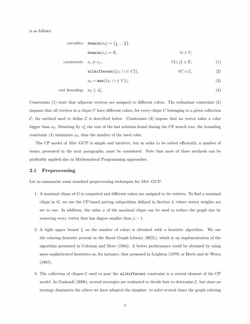
is as follows:
variables: domain(x0) = {χ . . . χ},
domain(xi) = K, ∀i ∈ V,
constraints: xi 6= xj , ∀{i, j} ∈ E, (1)
alldifferent({xi | i ∈ C}), ∀C ∈ C, (2)
x0 = max({xi | i ∈ V }), (3)
cost bounding: x0 ≤ x∗0. (4)
Constraints (1) state that adjacent vertices are assigned to different colors. The redundant constraint (2)
imposes that all vertices in a clique C have different colors, for every clique C belonging to a given collection
C; the method used to define C is described below. Constraints (3) impose that no vertex takes a color
bigger than x0. Denoting by x∗0 the cost of the last solution found during the CP search tree, the bounding
constraint (4) minimizes x0, thus the number of the used color.
The CP model of Min–GCP is simple and intuitive, but in order to be solved efficiently, a number of
issues, presented in the next paragraphs, must be considered. Note that most of those methods can be
profitably applied also in Mathematical Programming approaches.
2.1 Preprocessing
Let us summarize some standard preprocessing techniques for Min–GCP.
1. A maximal clique of G is computed and different colors are assigned to its vertices. To find a maximal
clique in G, we use the CP-based pricing subproblem defined in Section 4, where vertex weights are
set to one. In addition, the value ω of the maximal clique can be used to reduce the graph size by
removing every vertex that has degree smaller than ω − 1.
2. A tight upper bound χ on the number of colors is obtained with a heuristic algorithm. We use
the coloring heuristic present in the Boost Graph Library (BGL), which is an implementation of the
algorithm presented in Coleman and More (1984). A better performance could be obtained by using
more sophisticated heuristics as, for instance, that proposed in Leighton (1979) or Hertz and de Werra
(1987).
3. The collection of cliques C used to post the alldifferent constraint is a crucial element of the CP
model. In Gualandi (2008), several strategies are evaluated to decide how to determine C, but since no
strategy dominates the others we have adopted the simplest: to solve several times the graph coloring
5
problem on the complementary graph G with the heuristic in the BGL, randomly shuffling the order
of the vertices. Each class of colors in G corresponds to a clique of G.
2.2 Upper and lower bounding via CP
When solving model (1)–(3), there are two alternative options for the CP labeling strategy of variable x0:
(i) x0 is not considered as a branching variable, thus constraint (3) determines the value of x0 only when all
the other variables xi (with i > 0) have been assigned, or (ii) variable x0 is a branching variable.
In the first case, a Branch-and-Bound using the cost-bounding constraint (4) yields solutions with de-
creasing costs. We call this strategy CP–UB, since it provides a sequence of upper bounds even if the search
is stopped before the search tree has been completely explored. In the second case, we can consider the
following two-level labeling strategy: in the first level, we assign to variable x0 the minimum value v′ in its
domain, then, in the second level, we label all the other xi variables. In this way, the first solution found
by the CP solver is the optimum one, and the search can stop. Note that, in this case, the cost-bounding
constraint (4) is not needed. In addition, each time the second level labeling strategy has to backtrack to
the first level in order to assign a new value to variable x0, it means that a k coloring with k = v′ does not
exist, thus the lower bound increases. We call this second strategy CP–LB, since if it is stopped before the
search tree has been completely explored, the current value of x0 is the best lower bound.
2.3 Symmetry Breaking
Min–GCP is a challenging problem partially due to the high number of symmetric solutions. While fixing
the colors of a maximal clique breaks statically a certain number of symmetric solutions in the preprocessing,
many more symmetries arise during the solution of problem (1)–(4). In general the same criterion can be
applied at each labeling phase. Consider the set of variables with an undetermined value and such that their
domains have null intersection with the set of assigned colors, and let C ′ be a clique of the corresponding
vertices of G. As it is done in the preprocessing phase, we can avoid to generate branches on the assignment
of these variables and we can directly assign them a different color selecting it from their domain. The
simplest and less time consuming method is to consider cliques of one vertex, which allows in any case to
significantly reduce the number of search nodes in a reasonable time.
Other symmetry breaking strategies have been proposed in the literature (e.g. Gent et al., 2006). They
are computational more demanding and more complex to be implemented. Since the evaluation of their
utility goes beyond the scope of this work, we decided to leave their use for future investigation.
6
3 Graph Coloring via Branch-and-Price
Min–GCP can be also seen as the problem of partitioning the vertices of a graph into the minimum number
of stable sets, since all stable set vertices can be assigned to the same color, no matter which. Being a
minimization problem, Min–GCP can be formulated as a set covering where the ground set is given by
V and the family of subsets is the collection of maximal stable sets of G. Alternatively, a set packing
formulation of Min–GCP is presented in Hansen et al. (2009), but since it yields the same lower bound than
the set covering formulation, we consider here only the former.
Let S be the collection of all maximal stable sets of G = (V,E), and Sv be the collection of maximal stable
sets containing v ∈ V . Denoting by λi the selection variable of stable set i, the set covering formulation of
Min–GCP is:
zMP = min∑i∈S
λi (5)
s.t.∑i∈Sv
λi ≥ 1, ∀v ∈ V, (6)
λi ∈ {0, 1}, ∀i ∈ S. (7)
In a Column Generation scheme, we consider the so called restricted master problem:
zRMP = min∑i∈S
λi (8)
s.t.∑i∈Sv
λi ≥ 1, ∀v ∈ V, (9)
λi ∈ [0, 1], ∀i ∈ S. (10)
where S ⊆ S is such that the existence of a feasible solution is guaranteed, that is S is a subset of maximal
stable sets such that each vertex v of G is contained in at least one set of S. Let zMP denote the linear
relaxation optimal solution value of problem (5)–(7). Note that zMP is equal to the chromatic number χ(G),
and that zMP is equal to the fractional chromatic number χf (G). The computation of χf (G) is an important
NP-hard problem, and it gives the sharpest known lower bound for χ (Schrjiver, 2008).
Consider the dual of problem (8)-(10) where we denote by πv the dual variables of constraints (9). Given
the optimal dual solution πv, to check the existence of negative reduced columns to be added to (8)–(10),
the following pricing subproblem has to be solved:
s∗ = max∑v∈V
πvyv (11)
s.t. yv + yw ≤ 1, ∀{v, w} ∈ E, (12)
yv ∈ {0, 1}, ∀v ∈ V. (13)
7
Note that this problem is equivalent to finding the maximum weight stable set: variable yv is equal to one if
vertex v is part of the stable set and constraints (12) avoid that neighbors of v are in the solution. Negative
reduced cost columns correspond to solutions of problem (11)–(13) with value strictly greater than 1, thus
the actual value of the pricing subproblem is c∗ = 1 − s∗. The pricing subproblem (11)–(13) is solved in
Mehrotra and Trick (1996) with a recursive algorithm that could be used both as an exact and a heuristic
method. In the heuristic case, the execution is stopped when a stable set with s∗ > 1.1 (i.e. c∗ < −0.1) is
found.
If the pricing subproblem is solved with an exact method, the value zRMP
1−c∗ is a valid lower bound on
zMP , as shown in Lubbecke and Desrosiers (2005). This bound can be used to early terminate the column
generation algorithm whenever dzRMP e = d zRMP
1−c∗ e.
4 Constraint Programming-based Column Generation
The main idea of the CP–CG framework is to use CP to formulate and solve the pricing subproblem.
The use of CP is sound since it is not necessary to solve the pricing subproblem to optimality, but it
suffices to find a negative reduced cost solution. In order to formulate the pricing subproblem with CP,
the negativeReduceCost global constraint has been introduced in Fahle et al. (2002). Let Y be a set
variable having domain ranging into the vertex set V , and let τ ≤ 0 be a parameter. In our context, the
negativeReducedCost(π, Y, τ, c) symbolic constraint forces the set of vertices in Y to define a column with
reduced cost smaller than τ . Fixing the value of τ to 0 is equivalent to look for any negative reduced cost
column. This way, the general CP model of the pricing decision subproblem is:
variables/domains: Y ⊆ V, (14)
domain(Xi) ∈ {0, 1}, ∀i ∈ V, (15)
domain(c) < 0, (16)
constraints: negativeReducedCost(π, Y, 0, c), (17)
Xi +Xj ≤ 1, ∀{i, j} ∈ E, (18)
Xi = 1⇔ i ∈ Y, ∀i ∈ V, (19)
cost bounding: c0 ≤ c∗0. (20)
Constraints (17) is implemented as a weighted maximum clique constraint, that forces the vertices in Y to
be a clique of the complement G of G, i.e., a stable set of G, with cost at least equal to τ . Constraints (18)
are equivalent to constraints (12). Constraints (19) link the binary variables Xi with the set variable Y .
8
The CP pricing can be solved either as a decision problem or as an optimization problem. In the first case,
it is enough to solve problem (14)–(19) to obtain an improving column for the restricted master problem. In
the second case, the cost variable c is used as an optimization variable. During the search process, each time
the CP solver finds a solution of cost c∗, a bounding constraints c ≤ c∗−1 is added until optimality is proven.
In the context of CP–CG, the use of optimization constraints that perform cost-based domain reduction is
of particular interest for enhancing the filtering of the negativeReduceCost constraints. For further details
on the CP solving techniques and on more involved CP search strategies, see Milano and Wallace (2006).
We define some quality measures of columns added to the restricted master problem during the Column
Generation process in order to account for their impact in the solution of the linear relaxation and of the
integer problem. Let a be a column with negative reduced cost equal to c′, and let c∗ be the optimum value
of the pricing subproblem.
Definition 1 The relative reduced cost γ of column a with respect to (8)–(10) is
γ =c′
c∗.
Definition 2 Column a is γ-LP-good if it has a relative reduced cost γ > 0.
Solving the optimization version of the pricing subproblem is equivalent to generate 1-LP-good columns.
Let z0RMP be the optimum of the integer restricted master problem (8)–(9) with 0–1 variables λi without
column a, and let z′RMP be the optimum of the same integer master problem but extended by column a.
Definition 3 The integer impact factor δ of column a with respect to (8)–(9) with 0–1 variables λi is
δ =z0RMP − z′RMP
z0RMP
.
Definition 4 Column a is δ-IP-good if it has an integer impact factor δ > 0.
In a Column Generation approach γ-LP-good and δ-IP-good columns are important to improve the lower
bound and the upper bound, respectively. These issues have been addressed by several papers in the recent
literature. Further on, we present the related work while illustrating our enhancing strategies.
4.1 Weighted Maximum Clique Constraint
Constraint (17) plays a crucial role in the solution of the CP pricing subproblem. It might be implemented
as the naive sum over set constraint, but it would perform a rather weak propagation. Therefore, we have
extended the maximum clique constraint presented in Fahle (2002) to the case where vertices have positive
weights and we look for the maximum weighted clique.
9
The maximum clique constraint presented in Fahle (2002) basically works as follows. Two sets of vertices
are maintained: (i) the current partial solution C and (ii) the candidate set P , i.e., the set of vertices that
could extend C to a larger clique. A Branch-and-Bound algorithm selects the vertices from P to be added
to C; each time a vertex v ∈ P is moved into C, the candidate set is reduced as P ← P ∩N(v) \ C, where
N(v) is the set of vertices adjacent to v. An additional filtering algorithm removes from the set P all the
vertices having degree smaller than |C|. Despite its simplicity, this rule is very effective. Therefore, we have
adapted it to the weighted case. Let w(C) be the weight of the current clique. Then, the filtering algorithm
for the weighted case is: remove from the set P every vertex having the sum of the weights of its neighbors
plus its own weight smaller than w(C).
The maximum weighted constraint is used in a CP problem with an ad hoc labeling strategy that selects
from the candidate set P the vertex v maximizing the sum of vertex weights in N(v) ∩ P . In case of ties,
the vertex with highest degree is selected.
4.2 Generating γ-LP-good columns
The aim is to reduce the computation time required for solving the linear relaxation of master problem
(5)–(7) Note that the strategies that we are going to present are not tailored to graph coloring and can be
used also in other contexts.
4.2.1 Shuffled Static Order
In column generation, producing diverse columns is a desideratum, since diverse columns improve the con-
vergence rate of the algorithm, and mitigate the degeneracy phenomenon (Lubbecke and Desrosiers, 2005)
which unfortunately is quite common when CP is used to approach the pricing problem (Rousseau, 2004).
Indeed, during the iterations of the column generation algorithm, the pricing subproblem (14)–(17) does not
change, with the exception of coefficients π in the negativeReducedCost constraint. The decision variables
are stored in a vector y having always the same order corresponding to that of matrix A rows. Even if the
CP solver uses a dynamic ordering for labeling the variables, for instance the first-fail strategy, it will
always query them in vector y in the same order, typically from the lowest to the highest index. Therefore, if
the dynamic ordering heuristic has ties, independently from the way ties are broken and from how the search
tree is visited, variables with lower indices have more chances to be selected appearing more frequently in
the generated columns.
In order to avoid this phenomenon, several ideas have been proposed. For example in Sellmann et al.
(2002) variables selected more than k times are penalized in the labeling, or in (Rousseau, 2004) the Limited
Discrepancy Search (Harvey and Ginsberg, 1995) is used as a CP search strategy to implicitly generate
10
diverse columns. In contrast to Depth First Search, Limited Discrepancy Search is not a complete search
strategy and depends on a parameter, that is, the maximum number of allowed discrepancy whose value
may heavily affect the performance and that in practice is set by trial-and-error.
Our idea is to statically random shuffle variables indices of vector y at each iteration of the column
generation, before the CP solver begins the search phase. This shuffled static order acts as an implicit
random tie-breaking strategy. The effect of the shuffling is impressive: it produces very diverse columns as
a consequence of the constraint propagation, and it reduces dramatically the number of iterations of the
Column Generation (Gualandi, 2008). Note that the shuffled static order is straightforward to implement,
parameter-free and problem independent, moreover it is orthogonal to the search strategy.
The idea of using a random component in the search strategy is not completely new, but the way
and the purpose of its use are part of our contribution: the concern is not to speed-up the solution of a
single problem instance, but, given a set of instances of the same problem, to generate diverse solutions.
An iterative randomized search strategy that randomly selects variable-value pairs during the search is
presented in Gomes et al. (1998). The iterative randomized search is applied in Otten et al. (2006) obtaining
a considerable speed-up against usual deterministic search strategies. Though efficient, the iterative random
search strategy depends heavily on the parameter setting. The idea of the dual strategy presented in Gendron
et al. (2005) is close to that of the shuffled static order. The dual strategy selects first the variable having
the i-th smallest reduced cost, where i is a pseudo-random number, and it is used for generating multiple
columns at the same iteration of the column generation that is with the same dual multipliers π, rather than
generating diverse solution in different iterations.
4.2.2 Adaptive Thresholds for the Negative Reduced Cost Constraint
The solution of the pricing (11)–(13) as a decision problem through CP model (14)–(19) aims at generating
γ-LP-good columns limiting the computation effort. A solution of the pricing decision problem may have a
negative reduced cost slightly smaller than zero, yielding a modest improvement. If we knew the cost c∗ of
the pricing subproblem optimum solution, we could add to the CP model (14)–(19) the constraint c = c∗.
Since the value c∗ is not a priori known, our idea is to introduce an oracle that gives an estimate τ such that
c∗ ≤ τ < 0. If τ is equal to c∗, the solution of the decision problem is a 1-LP-good column and it has been
obtained without the need to prove optimality.
In practice, the idea is to alternate between the decision and the optimization pricing subproblems to
take advantage of the respective strengths. The pricing decision subproblem is faster since it can be arrested
whenever a solution with reduced cost lower than a given value τ is found. The pricing optimization problem
is useful to compute the following lower bound for the restricted master problem (Lubbecke and Desrosiers
11
(2005)):
κ(c∗) =zRMP
1− c∗ ≤ zMP . (21)
The underlying intuition of using a threshold τ is that we would like to obtain a new column potentially
yielding a lower bound improving the current one without solving the optimization pricing subproblem. The
idea of using a threshold is not new: for instance in Mehrotra and Trick (1996), the value of τ is empirically
fixed to 1.1. To the best of our knowledge, ours is the first attempt to determine the values of τ analytically,
and not experimentally by a trial-and-error hand-tuned strategy.
First threshold: exploiting an a priori known lower bound. Let κ be a given lower bound for zMP
and let κ(c∗) computed as in (21). There are two possibilities:
either κ ≤ κ(c∗) < zMP
or κ(c∗) < κ < zMP
In the first case, as κ(c∗) would yield a better lower bound than κ, the optimization pricing could be worth
solving. While, in the second case, this would be useless, since κ would be anyway the best lower bound.
Therefore, if the pricing subproblem finds a solution of cost c such that κ(c∗) ≤ κ(c) < κ, we could stop the
solution of the pricing subproblem, saving computation time.
Considering the Min–GCP setting, the idea is to look for a maximal stable set that attains a reduced
cost c < 0, and that satisfies the inequality:
κ(c∗) ≤ κ(c) =zRMP
1− c < κ < zMP (22)
Let z iRMP be the value of the restricted master problem at the i-th iteration, and let s denote the value of
the maximal stable set (i.e., c = 1 − s). Using the second and the third term in (22), the value of τ at the
i-th iteration is computed as follows:
zRMP
1− c < κ → c = 1− s = 1− ziRMP
κ→ s =
ziRMP
κ= τ(i). (23)
At the i-th iteration, if solving the pricing subproblem, we find a stable set of value s > τ(i) = ziRMP
κ , we
can stop since, even if we could find a solution of higher cost, we would not get a lower bound better than
κ. Therefore, in constraint (17), we can set the value of c equal to τ(i) computed as in (23), and solve the
decision problem (14)–(19).
Second threshold: exploiting the lower bound κ(c∗). Let j be the current iteration of the column
generation algorithm and be i a preceding one, i.e. i < j, when the optimization pricing subproblem (14)–
(20) has been solved yielding the lower bound κi(c∗) computed by (21). Let z jRMP be the value of the
12
Algorithm 1 CP-based Column generation using adaptive thresholds.In S : subset of maximal stable set SVar π : dual optimal multipliersVar κ(c∗) : lower bound on zMP
Var s : maximal stable set with negative reduced costVar τ : threshold for the negative reduced cost constraint
1: repeat2: {zRMP , π} ← solveRMP(S) . solve problem (8)–(10)3: τ ← computeThreshold . using either formula (23) or (24)4: s← solvePricingCP(π, τ) . solve problem (14)–(20)5: if s is empty then6: {c∗, s} ← solvePricing(π, 0) . if solved to optimality update κ(c∗)7: end if8: if s is not empty then9: S ← S ∪ s
10: end if11: until s is empty (or dzRMP e = dκ(c∗)e)
restricted master problem at the j-th iteration. Then in order to compute the value of τ , we replace κ with
κi(c∗) = z iRMP
c∗i in formula (23) as follows:
τ(i, j) =z jRMP
κi(c∗)=z jRMP
z iRMP
c∗i. (24)
Note that when the algorithm approaches the optimal solution z jRMP ' z iRMP , c∗ i ' 0, and consequently
the value of the estimate τ tends to 0. In addition, if a lower bound κ is given, the current lower bound
is κi(c∗) = max{κ, κi(c∗)}. The main difference between (23) and (24) is that the second is usually more
accurate, but it requires to solve the pricing subproblem to optimality. It is not always evident whether the
improved accuracy is worth the additional computational effort.
Embedding the estimate τ into column generation. The regular column generation algorithm ex-
tended by considering the threshold values is described by Algorithm 1. To guarantee the correctness the
following additional steps are necessary:
step 3: to compute the threshold τ according to either (23) or (24);
step 4: to solve the CP-pricing using τ in the negativeReducedCost constraint. This is achieved by the
procedure solvePricingCP that solves problem (14)–(20) with cost vector π and threshold τ ;
step 6: if using the threshold τ yields no solution, the pricing problem has to be solved either by replacing
τ with the value 0 in the negativeReducedCost constraint or by solving the pricing to optimality.
The procedure solvePricing either calls the procedure solvePricingCP or – for dense graph – calls
Cliquer to solve the pricing subproblem to optimality.
13
4.3 Generating δ-IP-good columns
The motivation for generating δ-IP-good columns is that solving the restricted master problem containing
the columns generated by the usual pricing techniques we could obtain a solution far away from the optimal.
Indeed, the pricing subproblem focuses on columns with negative reduced costs, thus potentially improving
the objective function of the linear relaxation of the master, but it usually gives no clues about the impact
on the integer problem.
The issue of generating good columns for either the linear or the integer master problem has been tackled
in Gendron et al. (2005), where two labeling strategies for solving the CP pricing subproblem are presented:
a dual strategy and a master strategy. The dual strategy consists in solving the CP pricing subproblem with
a static order of the variables based on the values of the dual variables, thus, according to our notation, it
focuses on generating γ-LP-good columns. The master strategy consists in adding constraints to the pricing
subproblem exploiting the structure of the master problem, thus it is a strategy for generating δ-IP-good
columns. Although the overall computation time is comparable with respect to the regular pricing, the
master strategy gives smaller integrality gap than the dual strategy. The dual strategy mainly suffers from
the tailing-in effect, that is the effect occurring in the first iterations of column generation when many
negative reduced cost columns are introduced without improvement, while the master strategy suffers from
the tailing-off effect, that is the very slow convergence towards the optimal solution of the relaxation, due
to the introduction of columns with very small negative reduced cost Lubbecke and Desrosiers (2005). The
conclusion in Gendron et al. (2005) is that a hybrid method combining the two strategies might be very
effective.
We propose to use an additional pricing subproblem, called augmented pricing, that takes a γ-LP-good
column and generates a set of δ-IP-good columns. The idea is to use two pricing subproblems: the first
generates γ-LP-good columns and the second generates δ-IP-good columns. The first subproblem is the
regular pricing and can be solved with any of the strategies presented previously. The second subproblem
called augmented pricing is based on the idea of generating a set of structured columns that together with
the column generated by the regular pricing contribute to define a feasible solution. The augmented pricing
can be modeled as a CP problem with constraints coming both from the master and the pricing subproblems.
Consider an integer k = κ, and the column ap generated by the regular pricing subproblem, the augmented
pricing problem looks for a κ-partition, thus an integer solution of the master problem, that includes the
14
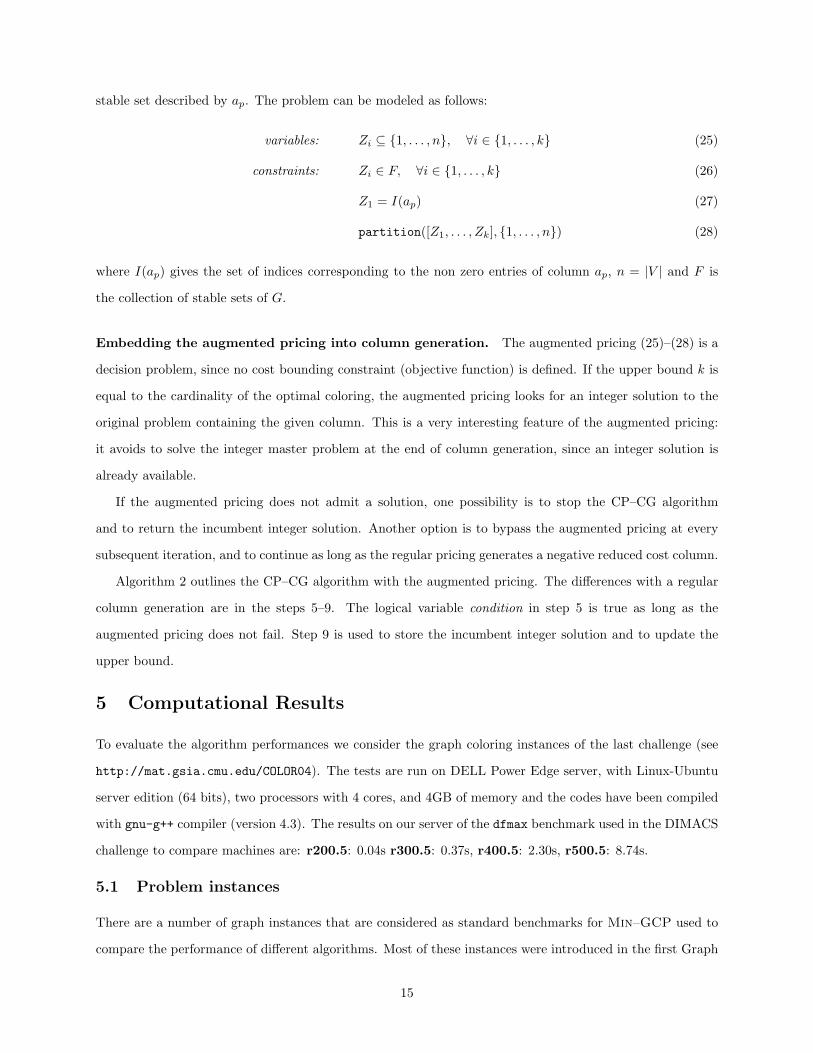
stable set described by ap. The problem can be modeled as follows:
There are a number of graph instances that are considered as standard benchmarks for Min–GCP used to
compare the performance of different algorithms. Most of these instances were introduced in the first Graph
15
Algorithm 2 Column generation with an augmented pricing.
In A : subset of feasible columns of AVar π : dual optimal values of the RMPVar κ, κ : integer lower and upper boundsVar ap, AP : improving columnsVar condition : boolean variableOut S : incumbent integer solution
1: repeat2: {zRMP , π} ← solveRMP(A) . solve problem (8)–(10)3: ap ← solveRegularPricing(π)4: if ap 6= ∅ then5: if condition then . strategy dependent6: AP ← solveAugmentedPricing(π, ap)7: end if8: if AP 6= ∅ then . in this case ap ∈ AP9: S ← AP ; κ← |AP | ; A← A ∪AP
10: else11: A← A ∪ ap; condition =false12: end if13: end if14: until ap = ∅ or dzRMP e = dκe
Coloring DIMACS challenge in 1994, and other instances were introduced during the second challenge held in
a series of workshops between 2002 and 2004. A number of instances from the first challenge are considered
easy, and do not provide significant information for comparing algorithms.
In this paper, we consider as easy all the instances that are solved to optimality by the Dsatur algorithm
within a timeout of two hours on our server. We have chosen the Dsatur algorithm, since it is used as
subroutine in other approaches, e.g., in Mendez-Dıaz and Zabala (2006). Table 2 lists all the easy instances
along with their number of nodes |V (G)| and edges |E(G)|, density d%, (maximal) clique number ω(G),
and chromatic number χ(G) (in italic when it is the best-known value). For instances having ω(G) < χ(G),
proving optimality is a non-trivial task.
We briefly describe the instances that are still challenging for exact methods. The first class of hard in-
stances are the random graphs DSJc.n.p introduced by Johnson. These instances correspond to standard ran-
dom graphs, where an edge between two vertices appears with probability equal to p. The DSJc.n.p instances
have probabilities equal to p = {0.1, 0.5, 0.9} and the number of vertices equal to n = {125, 250, 500, 1000}.Similar graphs are the Rn.p graphs introduced by Culberson, that are quasi-random graphs. The flat
instances were also introduced by Culberson, and are again very challenging. Another set of instances are
the Leighton graphs, all with 450 vertices, but with different clique numbers. The most difficult instances
are those with clique numbers equal to 15 and 25 (those with ω = 5 are easy). Then, there are the wap
instances, introduced by Koster, that are derived from frequency assignment problems, and are difficult due
16
to their size (around 1000 vertices).
Another type of challenging instances are those constructed so as to have an arbitrary large gap between
ω(G) and χ(G). The most famous are the Mycileski graphs, which have ω(G) = 2 and an arbitrary large
chromatic number. The myciel instances are quite easy to color. Though, it is very hard to prove opti-
mality. Similarly, the Insertions and FullIns graphs introduced by Caramia and Dell’Olmo, which are a
generalization of the Mycielski graphs, are easy to color, but it is hard to prove optimality.
Finally, there are few “isolated” challenging instances: abb313GPIA and ash608GPIA, arising in matrix
partitioning problems; and some latin square instances latin square 10, qgorder60 and qgorder100 that
are challenging due to their size.
5.2 CP approach
The CP approach presented in Section 2 is implemented in C++ using the Gecode 3.1 constraint system
(Schulte et al., 2009). The maximal clique used in the preprocessing is found with the Qualex-MS algorithm
(Busygin, 2006), a very efficient max-clique heuristic. The coloring heuristic used for the preprocessing is
part of the Boost Graph Library.
Table 2 compares the results obtained with the CP–UB and CP–LB approaches with the Dsatur algo-
rithm on the easy instances. For each method the table reports the computation time in seconds, and the
number of Branch-and-Bound nodes. Note the Dsatur algorithm is extremely fast on small graphs having
ω(G) = χ(G), but it takes more than 100 seconds on three instances (2-FullIns 3, le450 5d, and mug88 25)
and more than 3000 seconds on other three instances (1-Insertions 4, mug88 1, and quenn9 9). CP–UB
and CP–LB are never significantly worse than Dsatur both in terms of computation time and number
of Branch-and-Bound nodes, even if it is based on a general purpose solver, and perform much better for
Dsatur critical instances.
Table 3 reports the results of 11 instances that are solved within four minutes by the CP–LB approach,
but that are not solved within two hours by Dsatur. Among these instances, ash958GPIA and wap05 are
solved to optimality for the first time (with respect to the recent survey Malaguti and Toth (2010)), and
apart from the first two instances, the others are considered as hard instances in Mendez-Dıaz and Zabala
(2008). For the Dsatur algorithm, the table gives the UB found at the time limit. Note that for three
instances the upper bound is not even equal to the optimal solution, while CP–UB and CP–LB always return
the optimal solution.
17
Table 2: Instances solved by the CP–UB and CP–LB approaches within 1 minute. Comparison with theDsatur algorithm with a timeout of 7200 seconds.
CP-UB CP-LB Dsatur
Problem |V (G)| |E(G)| d% ω(G) χ(G) time B&B nodes time B&B nodes time B&B nodes
Table 3: Instances solved in about one minute by CP–LB. Comparison with CP–UB and Dsatur. Boldentries in column χ(G) denote instances optimally solved for the first time. Dsatur UB in italics denoteinstances where it differs from the optimal solution; for the other instances, Dsatur found the optimum butcould not certify it within 7200 secs (marked with ’-’).
CP-UB CP-LB Dsatur
Problem |V (G)| |E(G)| d% ω(G) χ(G) time B&B nodes time B&B nodes UB time
Preliminary experiments showed that most of the time of the column generation algorithm is spent in solving
the pricing subproblem, while solving the master takes a fraction of the whole time. Therefore, we decided
to focus on the number and the quality of the generated columns. While solving the optimization pricing
subproblem at each iteration does yield good columns reducing the number of iterations, the resulting overall
computation time is longer. To trade off the number of generated columns and their quality, we tested the
two rules to compute τ proposed in Section 4.2.2, comparing the results with those obtained fixing the
threshold as proposed in Mehrotra and Trick (1996).
The column generation approach given in Section 3 is implemented in C++ using CPLEX 12.1 as
Linear Programming solver, and using three different methods for the pricing subproblems. The pricing
decision subproblem is solved with an implementation of model (14)–(19) using Gecode 3.1, while the pricing
optimization subproblem is solved with Cliquer (Ostergard, 2002). On big and sparse instances, we have
also used the Qualex-MS algorithm (Busygin, 2006) for computing heuristic solutions. To compute the
initial set of stable sets S, we used the coloring heuristic part of the Boost Graph Library. The coloring
heuristic is executed a few times using different random vertex ordering, and all the classes of colors found
are stored in S. Note that before adding a class of colors to S, the corresponding stable set is increased to
a maximal one.
5.3.1 Adaptive thresholds
Table 4 compares the proposed strategies for setting the value of τ with the approaches found in the literature.
For each method, the table gives the number of generated columns and the computation time in seconds.
The timeout is set to 3600 seconds. Note that indeed a threshold different from 1.0 is necessary, otherwise a
19
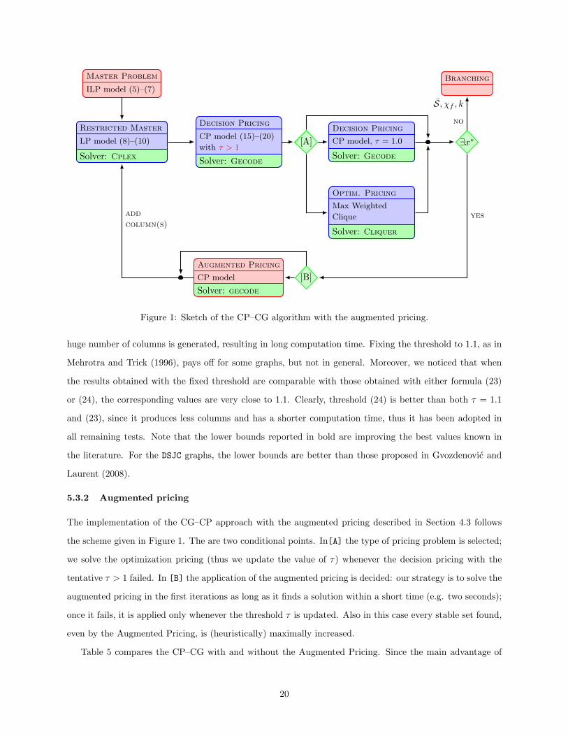
Master Problem
ILP model (5)–(7)
Branching
Restricted Master
LP model (8)–(10)
Solver: Cplex
Decision Pricing
CP model (15)–(20)
with τ > 1
Solver: Gecode
[A]Decision Pricing
CP model, τ = 1.0
Solver: Gecode
∃x∗
Optim. Pricing
Max Weighted
Clique
Solver: Cliquer
Augmented Pricing
CP model
Solver: gecode
[B]
yesadd
column(s)
no
S, χf , k
4
Figure 1: Sketch of the CP–CG algorithm with the augmented pricing.
huge number of columns is generated, resulting in long computation time. Fixing the threshold to 1.1, as in
Mehrotra and Trick (1996), pays off for some graphs, but not in general. Moreover, we noticed that when
the results obtained with the fixed threshold are comparable with those obtained with either formula (23)
or (24), the corresponding values are very close to 1.1. Clearly, threshold (24) is better than both τ = 1.1
and (23), since it produces less columns and has a shorter computation time, thus it has been adopted in
all remaining tests. Note that the lower bounds reported in bold are improving the best values known in
the literature. For the DSJC graphs, the lower bounds are better than those proposed in Gvozdenovic and
Laurent (2008).
5.3.2 Augmented pricing
The implementation of the CG–CP approach with the augmented pricing described in Section 4.3 follows
the scheme given in Figure 1. The are two conditional points. In[A] the type of pricing problem is selected;
we solve the optimization pricing (thus we update the value of τ) whenever the decision pricing with the
tentative τ > 1 failed. In [B] the application of the augmented pricing is decided: our strategy is to solve the
augmented pricing in the first iterations as long as it finds a solution within a short time (e.g. two seconds);
once it fails, it is applied only whenever the threshold τ is updated. Also in this case every stable set found,
even by the Augmented Pricing, is (heuristically) maximally increased.
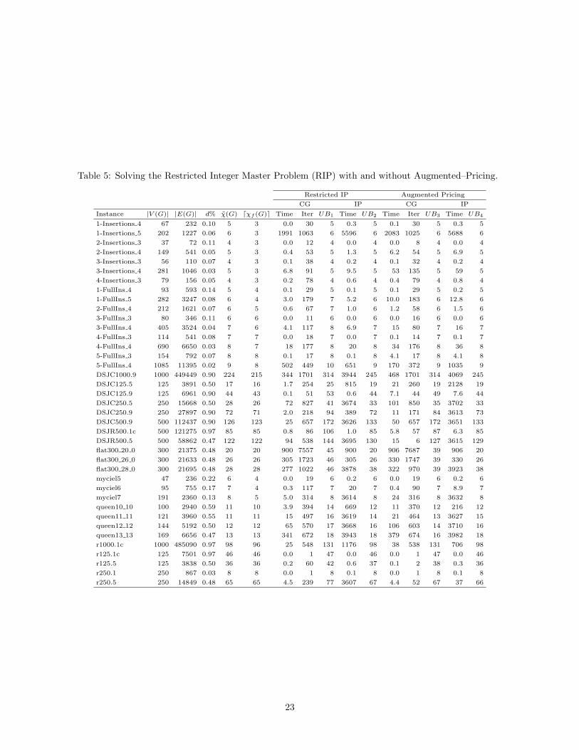
Table 5 compares the CP–CG with and without the Augmented Pricing. Since the main advantage of
20
Table 4: Comparing different strategies for threshold τ . Bold values in column dχg(G)e denote the new bestknown lower bounds. The times in bold point out the fastest approach. The timeout is set to 3600 secsdenoted by ’-’ when reached.
τ = 1.0 τ = 1.1 τ1 (23) τ2 (24)
Instance |V (G)| |E(G)| d% χ(G) dχf (G)e Iter Time Iter Time Iter Time Iter Time
This branching scheme is adopted in Mehrotra and Trick (1996), where an interpretation as a Ryan-Foster
(Ryan and Foster, 1981) branching is proposed. The advantage of this branching scheme is that at each
node of the Branch-and-Price tree we are facing an instance of Min–GCP, though on a different graph.
The critical issue of this branching scheme is how vertices v and w are selected. The branching used in
Mehrotra and Trick (1996) considers the stable set corresponding to the most fractional variable λ∗i of the
restricted master and another stable set corresponding to another column such that the two sets share a
vertex v and there is another vertex w belonging to one of the two sets only. We consider a similar selection
rule, but in choosing the second vertex w we break ties using the vertex degree.
Another critical issue in the Branch-and-Price algorithm is the order for visiting the nodes of the search
tree. Since the most important decisions are made in the first branching steps, i.e., the top of the search tree,
we have adopted an iterative depth-first search. That is, first, we fix a maximal depth; second, we entirely
visit the search tree up to the fixed depth; third, in case the search tree is not closed (by closing the lower
and upper bound gap) we increase the depth by one and restart the Branch-and-Price algorithm (almost)
from scratch. Note that every time the execution restarts, a new upper bound is computed. We could save
some computation time by storing the node that are still open at the given depth, but this would consume
much more memory, since the number of open nodes is exponential with the depth of the search tree. In
addition, in order to diversify the branching decisions each time the search restarts, we randomly generate
the columns of the initial pool of columns that form the initial feasible solution. Moreover, we use the ILP
solver also as a sort of primal heuristic: at each node of the search tree, we let CPLEX solve the restricted
master problem with a branch-and-bound node limit set to 100 (see, parameter MIP node limit in CPLEX
manuals), and with an upper bound set to the current upper bound -1.
Table 6 shows the results we obtain for some hard instances that in the recent survey of Malaguti and Toth
(2010) are reported as challenging for exact methods. The first six columns describe the instance features.
In addition, the column “BEUB.” gives the best results among those obtained with the exact methods, as
reported in Malaguti and Toth (2010). Note that DSJC125.5, DSJC125.9, DSJC500.1c, flat300 20 0, and
flat300 26 0 are solved to optimality for the first time with an exact method. For three other instances,
DSJC250.5, DSJC250.9, and DSJC500.9 we provide the best known lower bound obtained via column gen-
eration (see also Table 4) and the best upper bound obtained with an exact methods, though, for these last
three instances, meta-heuristics provide better upper bounds.
24
Table 6: Hard instances solved by our Branch-and-Price. Comparison with the best results found in theliterature with an exact method (column “BEUB”) as found in Malaguti and Toth (2010) and by heuristicalgorithms (column“bks”). Note that for the instances queen10 10 and queen11 11 the optimum values arereported in Vasquez (2004).
Min–GMP differs from Min–GCP because it requires that each vertex v is assigned to bv different colors,
i.e. to a given number of stable sets. Let S be the collection of all maximal stable sets in G = (V,E), and
Sv be the collection of maximal stable sets containing v ∈ V . The set covering formulation of Min–GMP
is:
zMP = min∑i∈S
λi (29)
s.t.∑i∈Sv
λi ≥ bv, ∀v ∈ V, (30)
λi ≥ 0, integer , ∀i ∈ S. (31)
Differently from Min–GCP formulation, here variables λi are integer and represent the number of times the
i-th class of colors is used in the solution. However, the pricing subproblem is the same as for Min–GCP, and
Min–GMP can be solved with the CP–CG approach given in Section 4 using (29)–(31) as master problem.
This approach was investigated in Mehrotra and Trick (2007) extending the work presented in Mehrotra and
Trick (1996).
Note that the graph reduction presented in Section 2.1 can be extended to Min–GMP: given the weight
ωm(G) of a maximum weighted clique, we can remove every vertex having the sum of the weights of its
neighbours plus its own weight smaller than ωm(G).
25
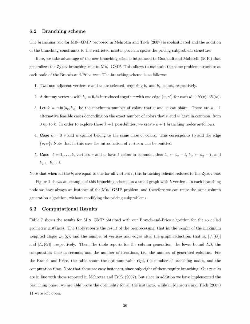
6.2 Branching scheme
The branching rule for Min–GMP proposed in Mehrotra and Trick (2007) is sophisticated and the addition
of the branching constraints to the restricted master problem spoils the pricing subproblem structure.
Here, we take advantage of the new branching scheme introduced in Gualandi and Malucelli (2010) that
generalizes the Zykov branching rule to Min–GMP. This allows to maintain the same problem structure at
each node of the Branch-and-Price tree. The branching scheme is as follows:
1. Two non-adjacent vertices v and w are selected, requiring bv and bw colors, respectively.
2. A dummy vertex u with bu = 0, is introduced together with one edge {u, u′} for each u′ ∈ N(v)∪N(w).
3. Let k = min{bv, bw} be the maximum number of colors that v and w can share. There are k + 1
alternative feasible cases depending on the exact number of colors that v and w have in common, from
0 up to k. In order to explore these k + 1 possibilities, we create k + 1 branching nodes as follows.
4. Case k = 0 v and w cannot belong to the same class of colors. This corresponds to add the edge
{v, w}. Note that in this case the introduction of vertex u can be omitted.
5. Case t = 1, . . . , k, vertices v and w have t colors in common, thus bv ← bv − t, bw ← bw − t, and
bu ← bu + t.
Note that when all the bi are equal to one for all vertices i, this branching scheme reduces to the Zykov one.
Figure 2 shows an example of this branching scheme on a small graph with 5 vertices. In each branching
node we have always an instance of the Min–GMP problem, and therefore we can reuse the same column
generation algorithm, without modifying the pricing subproblems.
6.3 Computational Results
Table 7 shows the results for Min–GMP obtained with our Branch-and-Price algorithm for the so–called
geometric instances. The table reports the result of the preprocessing, that is, the weight of the maximum
weighted clique ωm(g), and the number of vertices and edges after the graph reduction, that is, |Vr(G)|and |Er(G)|, respectively. Then, the table reports for the column generation, the lower bound LB, the
computation time in seconds, and the number of iterations, i.e., the number of generated columns. For
the Branch-and-Price, the table shows the optimum value Opt, the number of branching nodes, and the
computation time. Note that these are easy instances, since only eight of them require branching. Our results
are in line with those reported in Mehrotra and Trick (2007), but since in addition we have implemented the
branching phase, we are able prove the optimality for all the instances, while in Mehrotra and Trick (2007)
11 were left open.
26
1
2
3 4
5
(a) Initial graph: select vertices v = 2 andw = 4, with bv = 3 and bw = 2. Therefore,k = 2 is the maximum number of shared col-ors between v and w.
v
w
u
(b) The vertices v and w do not share anycolor. Vertex u, having bu = 0, is omittedalong with its incident edges.
v
w
u
(c) The vertices v and w share one color: weset bv = 2, bw = 1, and bu = 1.
v u
w
(d) The vertices v and w share two colors:we set bv = 1, bw = 0, and bu = 2. Vertex wis omitted.
Figure 2: Example of the branching rule for the Min–GMP problem: (a) the initial graph, and (b)–(d) thethree branching nodes, when the vertices 2 and 4 are selected for branching.
Table 8 reports the results obtained using the miscellaneous instances introduced in the DIMACS chal-
lenge. The best known results (column Bks) are obtained by taking the best results as reported in Mehrotra
and Trick (2007) and in Prestwich (2008). Note that 22 out of 40 instances are solved at the root node, since
the lower bound equals the upper bound. For 18 instances, branching is indeed necessary. 13 instances out
of 18 are solved to optimality with our Branch-and-Price algorithm. Remarkably, our algorithm requires a
small number of branching nodes for the instances that is able to solve. In addition, 13 instances are solved
to optimality for the first time.
Apparently most of Min–GMP literature instances are too small and relatively easy. For this reason
we generated a set of new more challenging instances derived from conflict graphs generated by the GLPK
Mixed Integer Linear Programming solver separating clique inequalities in solving MIPLIB2003 benchmarks.
Vertex weights are those assigned at the first call of the separation algorithm scaled and rounded in the range
[1..11]. We have omitted instances having more than 20000 vertices in the original graph and less than 60
vertices after preprocessing.
Table 9 shows the results obtained with our Branch-and-Price on the new COnflict Graph (COG)
instances. The first five columns describe each instance: note that the number of vertices can be very high,
while the density is always very small. Nevertheless, after the graph reduction based on the maximum
weighted clique (computed with Qualex), the resulting graphs are much smaller. In the new benchmarks,
there are four instances for which our Branch-and-Price algorithm reaches the timeout in the branching
phase, and five cases when the column generation algorithm does not even terminate at the root node. The
remaining 9 instances are solved to optimality. Our algorithm main difficulty emerges in the solution of
27
Table 7: Branch-and-Price results on the geometric instances. In bold the optimal results proved for thefirst time.
Preprocessing Column Generation Branch-and-Price
Instance |V (G)| |E(G)| d% |K| ωm(G) |Vr(G)| |Er(G)| LB Time Iter Opt. Nodes Time
the pricing subproblem. For example, for the COG-nsrand-ipx five iterations of the column generation,
corresponding to the solution of five pricing problems require one hour of computation.
7 Conclusions
We presented a computational study for Vertex Coloring Problems using two approaches Constraint Pro-
gramming and Column Generation, both as stand-alone methods and combined into a non-trivial hybrid
approach. A number of techniques improving the original implementations are also introduced. The result-
ing algorithms provide very interesting results on almost all the instances. Considering the Min–GCP in
particular, with respect with the best results presented in the literature and summarized in Malaguti and
Toth (2010), the main achievements can be summarized as follows:
1. CP–UB approach (or CP–LB, though with longer computation times) is able to prove the optimality
28
Table 8: Branch-and-Price results on several Min–GMP instances. In italics the upper bound of the openinstances, in bold the optimal results proved for the first time.
Preprocessing Column Generation Branch-and-Price
Instance |V (G)| |E(G)| d% |K| Bks ωm(G) |Vr(G)| |Er(G)| LB Time Iter UB Nodes Time