EXCEL 2007 Using Excel for Data Query & Management

IT Training & Development

(818) 677-1700

Training@csun.edu

http://www.csun.edu/training

Information Technology MS Office Excel 2007 Users Guide

Excel 2007 – Data Query & Management Page i

TABLE OF CONTENTS

Introduction ............................................................................................................................ 1

Freezing Panes ...................................................................................................................... 1

Keeping the Titles in View by Freezing Panes ..................................................................................... 1

Sorting Data ........................................................................................................................... 2

How Sorting Works ............................................................................................................................... 2

Sorting the Simple Way ........................................................................................................................ 3

Sort Orders ........................................................................................................................................... 3

Performing More Complex Sorting ....................................................................................................... 4

Changing the Sort Orientation .............................................................................................................. 5

Sorting by a Column That Contains Numbers or Text and Numbers ................................................... 6

How Excel Identifies Column Labels .................................................................................................... 6

Sorting a List That Does Not Have Column Labels .............................................................................. 6

Sorting Selected Data .......................................................................................................................... 6

How Filtering Works ............................................................................................................................. 7

Filtering a List Using a Simple Filter Command ................................................................................... 7

Removing a Filter ................................................................................................................................. 8

Filtering a Subtotaled List ..................................................................................................................... 8

Using Custom Criteria with AutoFilter .................................................................................................. 9

Creating And Removing Subtotals ........................................................................................10

Subtotals ............................................................................................................................................. 10

Data Validation ......................................................................................................................12

What is Data Validation? .................................................................................................................... 12

When is Data Validation Useful? ........................................................................................................ 12

Add Data Validation to a Cell or Range.............................................................................................. 12

The Data Validation Dialog Box ......................................................................................................... 13

Auditing Worksheets .............................................................................................................17

Display the Relationship between Formulas and Cells ...................................................................... 17

Using the Formulas Auditing Tools .................................................................................................... 18

Training And Support ............................................................................................................19

IT Training .......................................................................................................................................... 19

Microsoft on the Web ........................................................................................................................ 19

Excel 2007 – Data Query & Management Page ii of 26

Office 2007 Applications and Online Tutorials ................................................................................... 19

Troubleshooting and Support ............................................................................................................. 20

Excel 2007 – Data Query & Management Page 1 of 26

INTRODUCTION

Excel is a suburb data analysis tool if you know how to extract the information you really need. Learn how to obtain and locate the data you want. This guide provides the steps to follow so you can utilize some of the advanced features and tools within Excel.

FREEZING PANES

Keeping the Titles in View by Freezing Panes

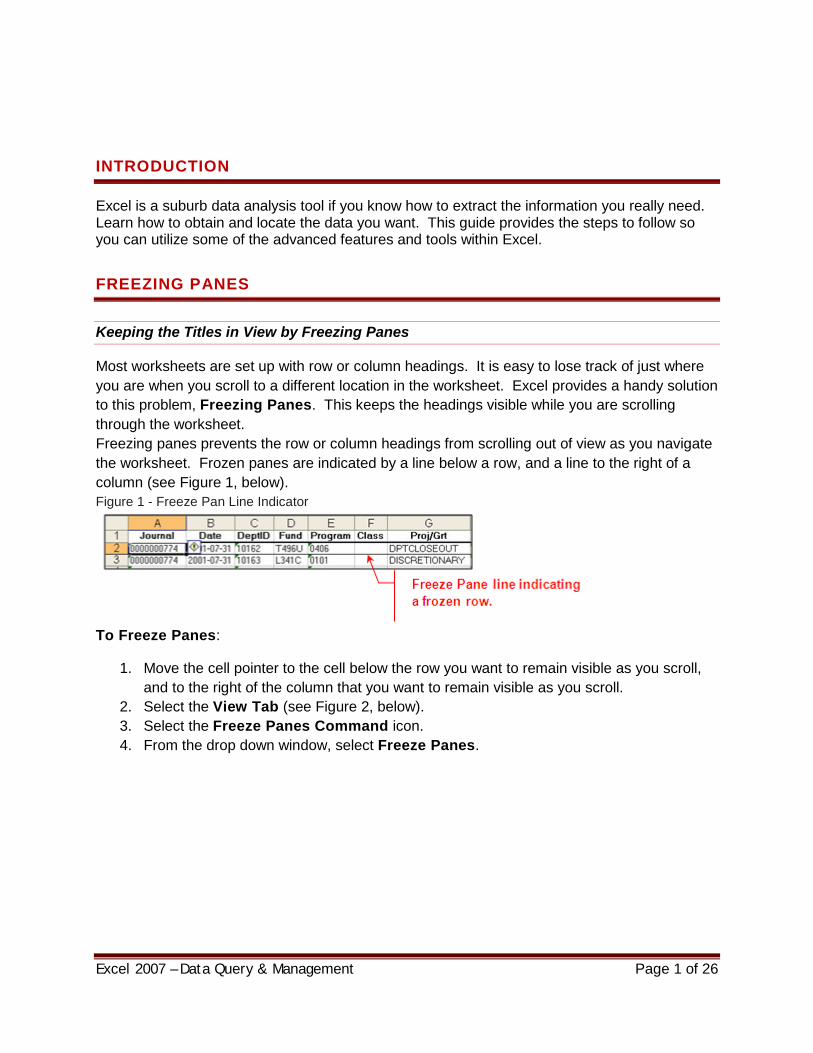
Most worksheets are set up with row or column headings. It is easy to lose track of just where you are when you scroll to a different location in the worksheet. Excel provides a handy solution to this problem, Freezing Panes. This keeps the headings visible while you are scrolling through the worksheet. Freezing panes prevents the row or column headings from scrolling out of view as you navigate the worksheet. Frozen panes are indicated by a line below a row, and a line to the right of a column (see Figure 1, below). Figure 1 - Freeze Pan Line Indicator

To Freeze Panes:

1. Move the cell pointer to the cell below the row you want to remain visible as you scroll, and to the right of the column that you want to remain visible as you scroll.

2. Select the View Tab (see Figure 2, below). 3. Select the Freeze Panes Command icon. 4. From the drop down window, select Freeze Panes.

Excel 2007 – Data Query & Management Page 2 of 26

Figure 2 - Selecting Freeze Pane from the View Tab

SORTING DATA

In some cases, the order of the rows in your list doesn’t matter. But in other cases, you want the rows to appear in a specific order. For example, in a personnel list, you may want the rows to appear in alphabetical order by last name. Or, if you have a list of expenditures, you may want to sort the list by date in ascending order.

Rearranging the order of the rows in a list is called Sorting. Excel is quite flexible when it comes to sorting lists, and you can often accomplish this task with the click of a mouse button.

Excel automatically treats any worksheet list as a database, allowing you to perform any of the commands on the Data menu. The rows serve as records, with columns serve as fields. When you have a data list in Excel, you can sort the list and filter the list to show only specific data

There are a few simple rules when creating your data list that you need to follow.

1. Include only one list per worksheet. 2. Include one blank column and one blank row between the list and any other

data in the worksheet. 3. Include column labels (titles) at the top of the list and format the labels (titles)

different from the rest of the data in the table. 4. Do not include any blank rows or columns in the data list.

How Sorting Works

When you sort a list, Microsoft Excel rearranges rows according to the contents of a column you choose - the Sort By column.

Excel 2007 – Data Query & Management Page 3 of 26

Sorting the Simple Way

The sort order is the way you want the data arranged. You can sort alphabetically or by value, and in ascending or descending order. For example, when you use an ascending sort order, numbers are sorted from 1 to 9, text is sorted from A to Z, and dates are sorted from earliest to latest.

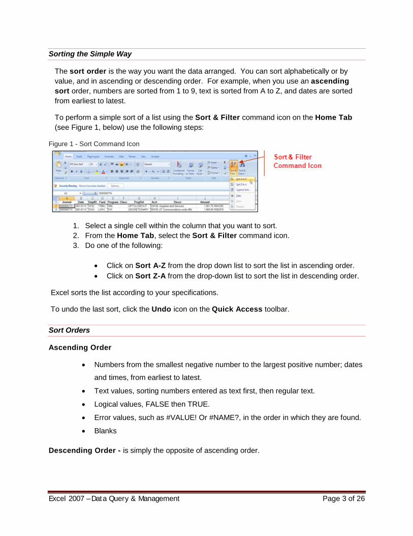
To perform a simple sort of a list using the Sort & Filter command icon on the Home Tab (see Figure 1, below) use the following steps:

Figure 1 - Sort Command Icon

1. Select a single cell within the column that you want to sort. 2. From the Home Tab, select the Sort & Filter command icon. 3. Do one of the following:

• Click on Sort A-Z from the drop down list to sort the list in ascending order. • Click on Sort Z-A from the drop-down list to sort the list in descending order.

Excel sorts the list according to your specifications.

To undo the last sort, click the Undo icon on the Quick Access toolbar.

Sort Orders

Ascending Order

• Numbers from the smallest negative number to the largest positive number; dates

and times, from earliest to latest.

• Text values, sorting numbers entered as text first, then regular text.

• Logical values, FALSE then TRUE.

• Error values, such as #VALUE! Or #NAME?, in the order in which they are found.

• Blanks

Descending Order - is simply the opposite of ascending order.

Excel 2007 – Data Query & Management Page 4 of 26

Restoring the Original Order of the List

If you want to perform a series of sorts and return the list to its original order:

1. Prior to beginning a sort, Insert a new column adjacent to the list.

2. Type “1: in the first cell beside the first row of information and “2’ in the second cell

beside the first row of information.

3. Use AutoFill to complete the consecutive numbering for the entire length of the list.

4. When you have completed the series of sorts, and want to return the list to its

original order, sort the numbered column in ascending order.

Performing More Complex Sorting

Sometimes, you may want to sort by two or more columns. Excel allows you to specify the priority of up to three columns by which you can sort the list. Figure 2 shows an example of an unsorted list.

Figure 2 - Sample of an Unsorted List

If you sort this list by date, Excel places the rows for each date together. But, you may also want to show the Department ID in ascending order within each date. In this case, you need to sort by at least two columns (Date and Department ID). Multiple column sorts require the use of the Custom Sort command on the Sort & Filter command icon drop-down list.

1. Select a cell in one of the columns in which you want to sort. 2. Select the Custom Sort option from the Sort & Filter command icon. Excel will

display the Sort dialog box (Figure 3, below).

Figure 3 - Custom Sort Dialog Window

Excel 2007 – Data Query & Management Page 5 of 26

3. In the Sort by field, select the down arrow. Excel will display the names of your column headings. Select the appropriate heading.

4. The Sort On field will default to Values. This will be the appropriate selection the majority of the time.

5. In the Order field, use the drop down arrow to select the appropriate sort. 6. Now, in the Then by field, select the next level of sort for your list. 7. To add additional levels to the sort, select the Add Level button (see Figure 4).

Complete each of the fields in the new level for sorting. 8. Click OK.

Figure 4 - Custom Sort Toolbar

If you have used the Sort command before, Excel displays the last column you selected. However, Excel recognizes the column headings, defaults to the left-most column heading, and places the column heading selections in the drop-down boxes.

Excel sorts the data in your list according to your specifications.

Note: If the sorting did not occur as you expected, select Edit > Undo (or press Ctrl + Z) to undo the sorting.

Changing the Sort Orientation

Excel allows you to change the sort orientation so that you can sort your information by rows rather than columns.

To change the sort orientation, use the following steps:

1. Select a cell in the row you want to sort. 2. Click on the Data tab and click on the Sort Command icon. 3. In the Sort dialog box click the Options button (see Figure 5, below).

Figure 5 - Sort Dialog Window Toolbar (Options Button)

Excel 2007 – Data Query & Management Page 6 of 26

4. Change the Orientation to Sort left to right. This will allow you to sort on a row. 5. Click OK. 6. In the Sort by field, select the down arrow. Excel will display the row number.

Select the appropriate row. 7. The Sort On field defaults to Values. This will be the appropriate selection the

majority of the time. 8. In the Order field, use the drop-down arrow to select the appropriate sort. 9. In the Then by field, select the next level; of sort for your list. 10. Click OK. Excel sorts the list according to your specifications.

Sorting by a Column That Contains Numbers or Text and Numbers

• If the Sort By column contains numbers, make sure the numbers are all in a numeric format, or are all formatted as text.

• If the column you want to sort by contains both numbers and numbers that include text characters (such as 100, 100a,), format them all as text if you want to sort them together. If you do not, Excel will sort the numbers first, then the numbers that include text (100, 200, 100a, 200a). To format a number as text, precede the number with an apostrophe ( ‘ ).

How Excel Identifies Column Labels

Microsoft Excel identifies labels by comparing the formatting in the top rows of your list. If there is a difference between the rows - - such as data type, capitalization, font alignment, or pattern - - Excel identifies the first row as column labels and excludes it from the sort. Excel can identify up to two rows or column labels.

Sorting a List That Does Not Have Column Labels

If there are no differences in data type, capitalization, font, alignment, or pattern between the first rows and the rows that follow, Excel will not identify column labels. Excel automatically selects the No Header Row option button under “My List Has” in the Sort dialog box. If for some reason, Excel identifies your first row as column labels but you want to include the row in the sort, manually select the No Header Row option button. You can then select a column to sort by using the generic column headings (Column A, Column B, and so on).

Sorting Selected Data

To sort only a subset of rows, or to sort the data in a single column of a list, first select the rows or columns you want to sort before you choose the Sort command. If you select data in a single column or row, Excel displays a message asking you to confirm that you want to sort only the selected cells. If you select Continue with the Current Selection and complete the sort, Excel sorts only the selected data, leaving the surrounding data in place.

Excel 2007 – Data Query & Management Page 7 of 26

Note: Sorting selected data does not move data in adjacent columns or rows.

How Filtering Works

Filtering is a quick and easy way to find and work with a subset of data in a list. When you filter a list, Excel displays only those rows that meet a set of search conditions called criteria.

• Filtering does not rearrange a list

• Filtering temporarily hides rows you do not want displayed.

There are two ways to filter a list in Excel:

• Simple Filter - Select the criteria to filter on.

• Customizing the Filter - Use Text Filters or Custom AutoFilters to narrow your search

criteria.

When you are in Filter mode, you can edit, format, chart, and print your list subset without rearranging or moving it.

Filtering a List Using a Simple Filter Command

1. From the Home tab, select the Sort & Filter Command icon (see Figure 6, below).

Figure 6 - Selecting Filter Command

2. Click Filter on the sub menu (see Figure 6, above). 3. Filter arrows appear at each column (see Figure 7, below).

Figure 7 - Filter Arrows at Each Column

Excel 2007 – Data Query & Management Page 8 of 26

4. Click the Filter arrow for the column of data you want to filter. An option box displays (see Figure 8, below).

Figure 8 - Filter Options Box

5. Excel lists each, unique entry for the selected column in the Text Filters area. De-select the unwanted entries so that only those entries you wish to see are checked.

6. Click OK.

Excel filters the data based on the criteria specified. All unmatched criteria are hidden. Note that the Arrow icon on the filtered column has changed (see Figure 9, below).

Figure 9 - Changed Filter Arrow Button

7. To bring the data back or to un-filter the data, select the Select All option from the filter drop-down selection.

Removing a Filter

• To remove filter criteria for a single column, select Select All from the column’s drop-down list.

• To remove Filter mode, select the Home tab > Sort & Filter command button > Filter.

Filtering a Subtotaled List

• Excel does not recalculate automatic subtotals when you filter. • Sort & Filter your list prior to using automatic subtotals.

Excel 2007 – Data Query & Management Page 9 of 26

Using Custom Criteria with AutoFilter

Each individual column can specify custom criteria.

This is useful when you want to:

• Display rows that contain either two items in a text field, such as rows that contain the account number for staff salaries and rows that contain the account number for management and supervisory salaries all under the Account column.

• Display rows that contain values that fall within a range of values such as rows that contain expenditures greater than 5,000 and less than 10,000.

To perform a custom criteria filter:

1. From the Filter Arrow, choose Text Filters OR Numbers Filters from the drop-down list (see Figure 10, below).

Figure 10 - Filter Menu

2. Select the custom criteria, by selecting the comparison operator you want to use. Such as greater than or equal to.

3. The Custom AutoFilter dialog box appears. 4. Specify the criteria. If you specify two custom criteria, choose how you want Excel to

apply the criteria.

Note: Excel allows you to filter with a Single Criterion or a Multiple Criterion.

Excel 2007 – Data Query & Management Page 10 of 26

CREATING AND REMOVING SUBTOTALS

Subtotals

Automatically calculate subtotals and grand totals in a list for a column by using the Subtotal command in the Outline group on the Data tab.

Subtotals are calculated with a summary function, such as Sum or Average, by using the Subtotal function. You can display more than one type of summary function for each column.

Grand Totals are derived from detail data, not from the values in a subtotals. For

example, if you use the Average summary function, the grand total row displays an average of all detail rows in the list, not an average of the values in the subtotal rows.

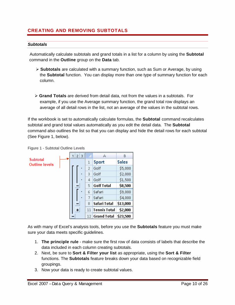
If the workbook is set to automatically calculate formulas, the Subtotal command recalculates subtotal and grand total values automatically as you edit the detail data. The Subtotal command also outlines the list so that you can display and hide the detail rows for each subtotal (See Figure 1, below). Figure 1 - Subtotal Outline Levels

As with many of Excel’s analysis tools, before you use the Subtotals feature you must make sure your data meets specific guidelines.

1. The principle rule - make sure the first row of data consists of labels that describe the data included in each column creating subtotals.

2. Next, be sure to Sort & Filter your list as appropriate, using the Sort & Filter functions. The Subtotals feature breaks down your data based on recognizable field groupings.

3. Now your data is ready to create subtotal values.

Excel 2007 – Data Query & Management Page 11 of 26

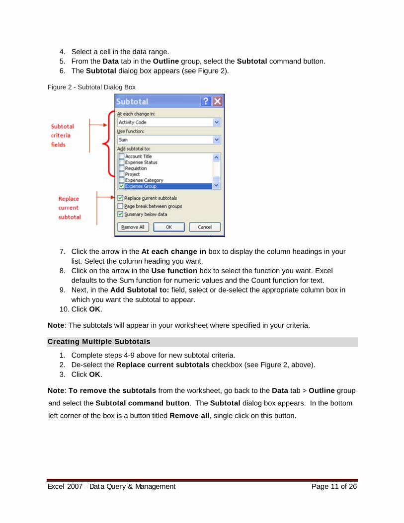
4. Select a cell in the data range. 5. From the Data tab in the Outline group, select the Subtotal command button. 6. The Subtotal dialog box appears (see Figure 2).

Figure 2 - Subtotal Dialog Box

7. Click the arrow in the At each change in box to display the column headings in your list. Select the column heading you want.

8. Click on the arrow in the Use function box to select the function you want. Excel defaults to the Sum function for numeric values and the Count function for text.

9. Next, in the Add Subtotal to: field, select or de-select the appropriate column box in which you want the subtotal to appear.

10. Click OK.

Note: The subtotals will appear in your worksheet where specified in your criteria.

Creating Multiple Subtotals

1. Complete steps 4-9 above for new subtotal criteria. 2. De-select the Replace current subtotals checkbox (see Figure 2, above). 3. Click OK.

Note: To remove the subtotals from the worksheet, go back to the Data tab > Outline group

and select the Subtotal command button. The Subtotal dialog box appears. In the bottom

left corner of the box is a button titled Remove all, single click on this button.

Excel 2007 – Data Query & Management Page 12 of 26

DATA VALIDATION

What is Data Validation?

Data validation is an Excel feature that you can use to define restrictions on what data can or should be entered in a cell. You can configure data validation to prevent users from entering data that does not meet your criteria. Messages can also be provided to define the input expected for a cell as well as instructions to help users correct any errors.

When is Data Validation Useful?

Data validation is invaluable when you want to share a workbook with others in your organization, and you want the data entered in the workbook to be accurate and consistent.

Add Data Validation to a Cell or Range

To create a validation rule:

1. From the Data tab, in the Data Tools group, click on the Data Validation command button (see Figure 1, below).

2. Excel will display the Data Validation dialog box (see Figure 2, below).

Figure 1 - Data Tab and Tools Grouping

Figure 2 - Data Validation Dialog Box

Excel 2007 – Data Query & Management Page 13 of 26

The Data Validation dialog box is used to define the type of data that Excel should allow in the cell and then, depending on the data type you choose, to set the conditions data must meet to be accepted in the cell.

For example: a column is set up to enter a person’s phone number and someone tries to enter the person’s name instead. By setting up accurate validation rules, the cell will only accept numeric values.

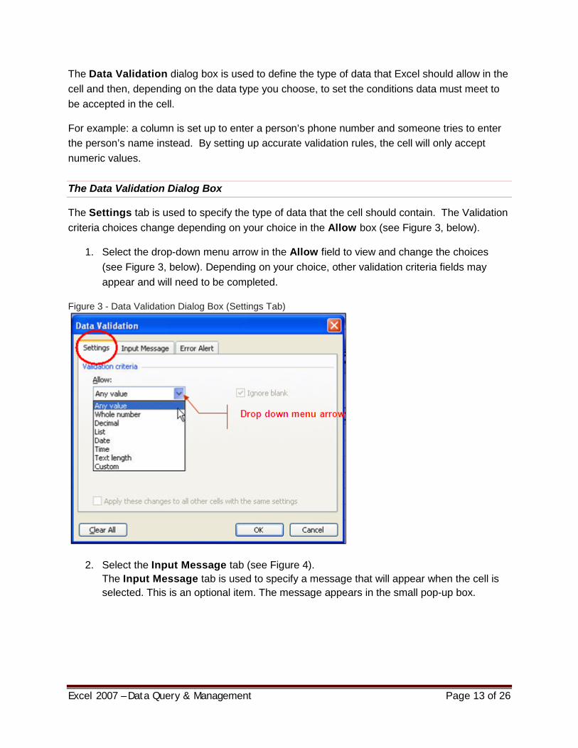
The Data Validation Dialog Box

The Settings tab is used to specify the type of data that the cell should contain. The Validation criteria choices change depending on your choice in the Allow box (see Figure 3, below).

1. Select the drop-down menu arrow in the Allow field to view and change the choices (see Figure 3, below). Depending on your choice, other validation criteria fields may appear and will need to be completed.

Figure 3 - Data Validation Dialog Box (Settings Tab)

2. Select the Input Message tab (see Figure 4). The Input Message tab is used to specify a message that will appear when the cell is selected. This is an optional item. The message appears in the small pop-up box.

Excel 2007 – Data Query & Management Page 14 of 26

Figure 4 - Data Validation Dialog Box (Input Message Tab)

Excel lets you create messages that tell the user what values are expected before data is entered. If the conditions are not met, it will reiterate the conditions in a custom error message when the Error Alert tab criteria fields are completed (see Figure 5, below).

Figure 5 - Input Message for Data Validation (Sample)

3. Title field - Enter a title for the message (see Figure 5, above). 4. Enter the message in the Input message: field.

Excel 2007 – Data Query & Management Page 15 of 26

Figure 6 - Sample of Validation Results after Message Input

5. To add the error message, select the Error Alert tab (see Figure 7). The Error Alert tab is used to specify the message that will appear in a dialog box if invalid data is entered. This is optional.

Figure 7 - Data Validation Box (Error Alert Tab)

6. There are four different components to complete. Each field is optional. • The Show error alert after invalid data is entered checkbox. • Style: field - offers three options for warning style. • Title: field - enter title or warning here. • Error message: field - enter the text that you want to appear.

Excel 2007 – Data Query & Management Page 16 of 26

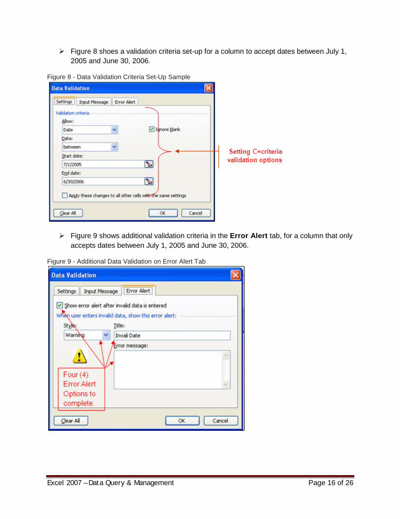
Figure 8 shoes a validation criteria set-up for a column to accept dates between July 1, 2005 and June 30, 2006.

Figure 8 - Data Validation Criteria Set-Up Sample

Figure 9 shows additional validation criteria in the Error Alert tab, for a column that only

accepts dates between July 1, 2005 and June 30, 2006.

Figure 9 - Additional Data Validation on Error Alert Tab

Excel 2007 – Data Query & Management Page 17 of 26

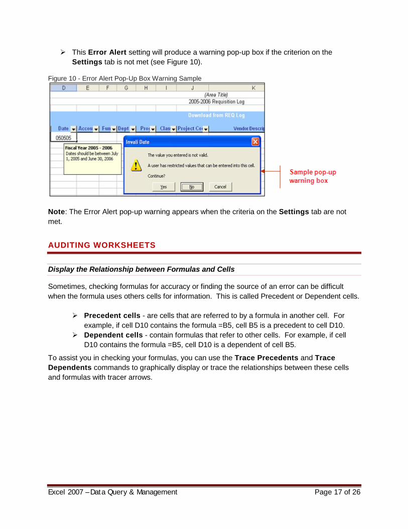
This Error Alert setting will produce a warning pop-up box if the criterion on the Settings tab is not met (see Figure 10).

Figure 10 - Error Alert Pop-Up Box Warning Sample

Note: The Error Alert pop-up warning appears when the criteria on the Settings tab are not met.

AUDITING WORKSHEETS

Display the Relationship between Formulas and Cells

Sometimes, checking formulas for accuracy or finding the source of an error can be difficult when the formula uses others cells for information. This is called Precedent or Dependent cells.

Precedent cells - are cells that are referred to by a formula in another cell. For example, if cell D10 contains the formula =B5, cell B5 is a precedent to cell D10.

Dependent cells - contain formulas that refer to other cells. For example, if cell D10 contains the formula =B5, cell D10 is a dependent of cell B5.

To assist you in checking your formulas, you can use the Trace Precedents and Trace Dependents commands to graphically display or trace the relationships between these cells and formulas with tracer arrows.

Excel 2007 – Data Query & Management Page 18 of 26

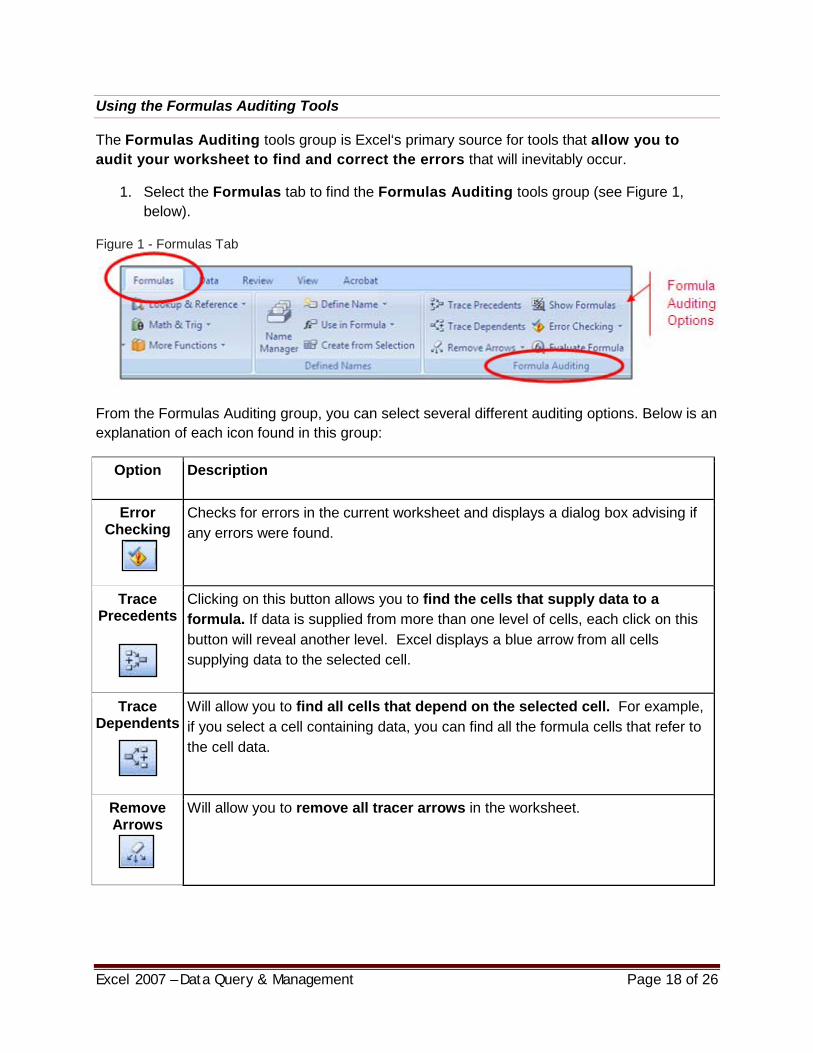
Using the Formulas Auditing Tools

The Formulas Auditing tools group is Excel‘s primary source for tools that allow you to audit your worksheet to find and correct the errors that will inevitably occur.

1. Select the Formulas tab to find the Formulas Auditing tools group (see Figure 1, below).

Figure 1 - Formulas Tab

From the Formulas Auditing group, you can select several different auditing options. Below is an explanation of each icon found in this group:

Option Description

Error Checking

Checks for errors in the current worksheet and displays a dialog box advising if any errors were found.

Trace Precedents

Clicking on this button allows you to find the cells that supply data to a formula. If data is supplied from more than one level of cells, each click on this button will reveal another level. Excel displays a blue arrow from all cells supplying data to the selected cell.

Trace Dependents

Will allow you to find all cells that depend on the selected cell. For example, if you select a cell containing data, you can find all the formula cells that refer to the cell data.

Remove Arrows

Will allow you to remove all tracer arrows in the worksheet.

Excel 2007 – Data Query & Management Page 19 of 26

Show Formulas

Displays the actual formula in each designated cell instead of the formulas results.

Evaluate Formula

Displays the Evaluate Formula dialog box so that you can view the formula and formula results in the selected cell. If the cell contains a complex formula, you can evaluate individual sections of the formula independently.

TRAINING AND SUPPORT

IT Training

IT Training & Development offer training in many different applications at various skill levels.

See what is coming up over the next few months by checking our website at:

www.csun.edu/it/training Contact Us: IT Training & Development

Phone: (818) 677-1700 or x1700 (on campus)

Email: training@csun.edu

Microsoft on the Web

Microsoft on the Web (WWW.MICROSOFT.COM) provides links to Web locations where you can find out more about Microsoft Office 2007. It is a great resource for learning. You need Internet connectivity and a web browser to use of this feature.

Office 2007 Applications and Online Tutorials

Get Up To Speed with Excel 2007

http://office.microsoft.com/training/training.aspx?AssetID=RC100620751033

Quick Reference Card for Get Up To Speed with 2007

http://office.microsoft.com/training/training.aspx?AssetID=RP100766581033&CTT=6&Origin=RC100766511033

Excel 2007 – Data Query & Management Page 20 of 26

Worksheet Design Strategy

http://office.microsoft.com/en-us/excel/HA011082671033.aspx

Troubleshooting and Support

If you experience problems getting started with Office 2007 contact the Help Center at x1400 or helpcenter@csun.edu.

Excel 2007 – Data Query & Management Page 21 of 26

NOTES

Excel 2007 – Data Query & Management Page 22 of 26

NOTES

Excel 2007 – Data Query Management Updated 04/26/10

IT’s technology training guides are the property of California State University, Northridge. They are intended for non-profit educational use only. Please cite source when using this material.