62
(212) 405.1010 | [email protected] | Follow: @1010data | www.1010data.com Excel Reporting with 1010data

(212) 405.1010 | [email protected] | Follow: @1010data | www.1010data.com
Excel Reporting with 1010data

Excel Reporting with 1010data | Contents | 2
© 2017 1010data, Inc. All rights reserved.
Contents
Overview....................................................................................................... 3
Start with a 1010data query....................................................................... 5
Running your query using the Excel Add-in............................................ 8
Adding a static input to a dashboard..................................................... 12
Targeting the query results to the dashboard........................................15
Formatting the results on the dashboard............................................... 17
Adding a simple chart to the dashboard................................................ 21
Creating a static drop-down in the dashboard.......................................25
Incorporating a dynamic drop-down in the dashboard......................... 31
Adding another query to the dashboard.................................................41
Adding a button to run the queries.........................................................44
Charting the results dynamically on the dashboard..............................49
Using 1010data libraries and blocks....................................................... 56
Hiding worksheets and locking the workbook....................................... 60

Excel Reporting with 1010data | Overview | 3
Overview
1010data gives its users the ability to manipulate and analyze large amounts of data using a familiarspreadsheet interface. It is for that very reason that the 1010data GUI is known as the Trillion RowSpreadsheet. Many of our users also like to use Microsoft Excel for its widely-known functionality andits ability to create user-interactive dashboards. Because of that, we’ve made it very easy to createdashboards in Excel that can leverage the power and speed of data analysis using the 1010data engine. Infact, it is fairly simple to incorporate user-specified parameters in a query that is run on 1010data and havethe results displayed directly in an Excel dashboard with charts and conditional formatting.
Let's say we want to build a dashboard in Excel that displays the results of two 1010data queries. Onesimply aggregates total sales for a specified department and date range, while the other aggregates totalsales by date for the same department. We want to give the user the ability to specify the start and enddates for the date range and to select the department for which they want to see total sales figures. Inaddition, we want to give the user the choice to aggregate either by group description or by brand. Finally,we want to see visualizations of the results in the dashboard using Excel's charting capabilities.
When we're finished with this tutorial, we want our dashboard to look something like the following:
Though this may look a little complex, it is created via a number of simple steps that this tutorial will guideyou through:
• Start with a 1010data query that aggregates total sales for a specific department and date range• Run the 1010data query from Excel using the 1010data Excel Add-in• Add static inputs to the dashboard for the date range• Target the results of the query to the dashboard• Format the query results using basic and conditional formatting• Add a simple chart to the dashboard• Create a static drop-down to allow the user to select whether they want to aggregate on group
description or brand• Incorporate a dynamic drop-down to allow the user to select a particular department for the query• Add another query that aggregates total sales by date for the same department

Excel Reporting with 1010data | Overview | 4
• Add a button to run both queries from the dashboard• Chart the results of both queries dynamically on the dashboard• Incorporate the use of 1010data libraries and blocks• Hide the worksheets and lock the workbook
Let's build the dashboard one step at a time.
We'll use the 1010data Excel Add-in to run a 1010data query from Excel and download the results directlyinto an Excel worksheet. Let's start with a 1010data query.

Excel Reporting with 1010data | Start with a 1010data query | 5
Start with a 1010data query
Let's start off by building a query using 1010data's Trillion-Row Spreadsheet interface.
For our example, we'll use a Sales Detail table (retaildemo.salesdetail) that containsbillions of rows of transactional data, and we'll incorporate information from a Product Master table(retaildemo.products) that contains detailed information about all of our products.
Let's say we want to calculate the total sales from 01/01/2011 to 03/31/2011 for items in department 19and we want to group the results by the values in the Group Desc column of the Product Master table.So, our results would look something like:
To do this in the 1010data web interface, it would take just a few simple steps.
We'll start by selecting those rows in the Sales Detail table whose values in the Date column fall between01/01/2011 and 03/31/2011:
Note: We specify the date using YYYYMMDD format.
In the Product Master table, we'll select those rows whose Department is 19.
Excel Reporting with 1010data | Start with a 1010data query | 6
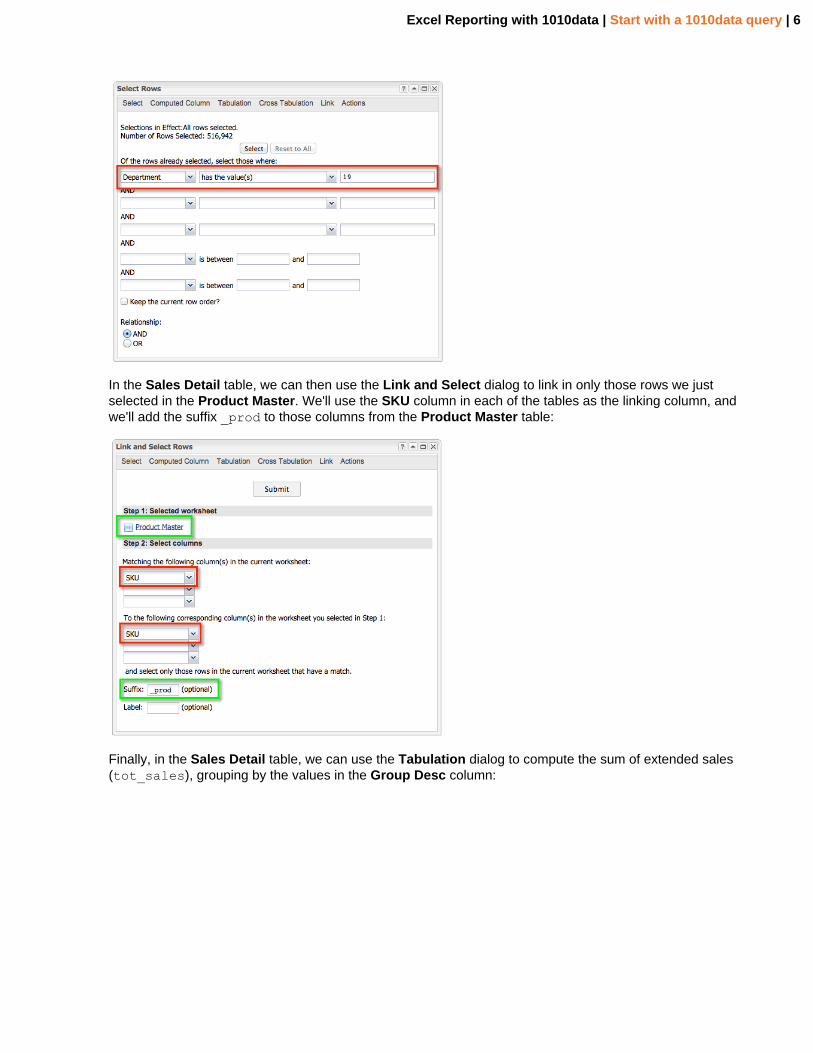
In the Sales Detail table, we can then use the Link and Select dialog to link in only those rows we justselected in the Product Master. We'll use the SKU column in each of the tables as the linking column, andwe'll add the suffix _prod to those columns from the Product Master table:
Finally, in the Sales Detail table, we can use the Tabulation dialog to compute the sum of extended sales(tot_sales), grouping by the values in the Group Desc column:

Excel Reporting with 1010data | Start with a 1010data query | 7
Click View > Edit Actions (XML)... to see the Macro Language code for our query:
We can then copy and paste this Macro Language code directly into the 1010data Excel Add-in.

Excel Reporting with 1010data | Running your query using the Excel Add-in | 8
Running your query using the Excel Add-in
Using the 1010data Excel Add-in, we can run a query on 1010data from Excel and have the results directlydownloaded into an Excel worksheet.
The Macro Language code for our example 1010data query is:
<note type="base">Applied to table: retaildemo.salesdetail</note><sel value="between(date;20110101;20110331)"/><link table2="retaildemo.products" col="sku" col2="sku" suffix="_prod" type="select"> <sel value="(dept=19)"/></link><tabu label="Tabulation on Sales Detail" breaks="groupdesc_prod"> <tcol source="xsales" fun="sum" name="tot_sales" label="Sum of`Extended Sales"/></tabu><sort col="tot_sales" dir="down"/>
To run this query in an Excel workbook, we can use the 1010data Excel Add-in.
Note: The 1010data Excel Add-in must be installed on your computer. (See Installing the 1010dataExcel Add-in for more information.) Once installed, you want to make sure that you have enabledthe advanced features of the 1010data Excel Add-in to perform the necessary steps in this tutorial.
In Microsoft Excel, from the Add-Ins menu, click 1010data > Add New Q-Sheet. This will open a q-sheetin a new tab labeled _1010q Sheet, which is where we will specify the query we want to run on 1010data.
Copy the Macro Language code for the 1010data query and paste it into the section of the q-sheet labeled1010data Macro Code.

Excel Reporting with 1010data | Running your query using the Excel Add-in | 9
We need to enter some other information in the q-sheet:
• For the Query Description, enter "Total Sales by Department".• In the To be Applied to Table field, we need to specify the full path to the table this query should be
applied to. For this example, we'll enter retaildemo.salesdetail.• In the Result Destination field, enter Sheet1!$A$1 so that the results will be pasted in cell A1 in the
Sheet1 worksheet.• From the Column Headers drop-down, select "Column Names".
Our q-sheet should look similar to the following:
Let's run the query and see our results. From the Add-Ins menu, click 1010data > Run Queries > InActive Workbook (or press Ctrl+Q).
Note: If you have not logged into 1010data via the Excel Add-in, you will be presented with thefollowing dialog:

Excel Reporting with 1010data | Running your query using the Excel Add-in | 10
Enter your 1010data credentials and click Secure Login.
As the query runs on 1010data, you'll see a 1010data Query Progress dialog, which shows thepercentage of total operations completed within the current query. When the query finishes running, youshould see a dialog saying: Query completed successfully. Click OK to dismiss this dialog.
To see the results, click the Sheet1 tab:
You can see that the results of this query have been downloaded into Excel and are the same as what wegot when we ran this query directly on 1010data.
Note: It's a good idea to save your workbook as you progress though this tutorial. Click File >Save As and navigate to the folder where you want to save your work. Be sure to select ExcelMacro-Enabled Workbook (*.xlsm) from the Save as type drop-down, as we will be incorporatingVBA macros later in this tutorial.

Excel Reporting with 1010data | Running your query using the Excel Add-in | 11

Excel Reporting with 1010data | Adding a static input to a dashboard | 12
Adding a static input to a dashboard
Our original query had date values hard-coded for the row selection. Let's add a little more flexibility byallowing the user to enter a date range using static inputs.
We'll create a dashboard where the user can enter the start and end dates for the date range, and thenwe'll use those values in the query.
We can use Sheet2 for our dashboard (or create a new worksheet, if necessary). Let's rename it"Dashboard" and change the background color to a light grey.
Enter text in the cells so that your dashboard looks similar to the following:
You can see in this example that we will allow the user to enter a start date in cell B3 and an end date incell B7. Below the inputs, we specify that we want the dates in the format YYYYMMDD, which is the dateformat used by 1010data.
Note: There are no restrictions as to what the user can enter in these cells. These are simplycells in which the user can type in any values. Also, though we are specifying that we want theuser to enter dates in the YYYYMMDD format for this example, you might want to allow the userto enter dates in a more recognizable format (e.g., MM/DD/YYYY). In this case, you would need todo some type of transformation on these input values to put them in the YYYYMMDD format. Thisdate transformation could be done in Excel before the values are passed to the query, or within the1010data query itself. (See Date Transformations for examples on how to do such a transformationwithin the 1010data query.)
Let's also name the cells that contain the start and end dates so that it will be easier to reference them inour q-sheet. We'll give the cell B3 the name startdate and the cell B7 the name enddate.
The q-sheet essentially sends whatever Macro Language code it contains to 1010data to process andreturn the results. Because of that, we can convert any row in the q-sheet that contains our macro codeinto an Excel formula that references the contents of other cells. Then, when the Excel Add-in sends thatquery to 1010data, it will contain the values in the referenced cells.
In our query, the date selection was done using the between(X;Y;Z) function:
<note type="base">Applied to table: retaildemo.salesdetail</note><sel value="between(date;20110101;20110331)"/><link table2="retaildemo.products" col="sku" col2="sku" suffix="_prod" type="select"> <sel value="(dept=19)"/></link><tabu label="Tabulation on Sales Detail" breaks="groupdesc_prod"> <tcol source="xsales" fun="sum" name="tot_sales" label="Sum of`Extended Sales"/></tabu><sort col="tot_sales" dir="down"/>

Excel Reporting with 1010data | Adding a static input to a dashboard | 13
Let's go over to our q-sheet and change the hard-coded date values in our query to reference the newinput values, startdate and enddate.
To reference input values from within the 1010data query, we will need to change the line in our macrocode into a formula. We do this by:
• removing any blank spaces from the start of the line• inserting an = at the beginning of the line• enclosing the macro code in double quotes• preceding any double quote within the macro code with another double quote so that Excel will not
interpret any of them as the end of the formula• replacing each hard-coded value with a reference to its corresponding input cell using the syntax:
"&[CELL_REFERENCE]&" (e.g., "&B3&")
Let's go through those steps for our example. There are no blank spaces at the start of the line, so we canmove to the next step and add an = to the beginning:
=<sel value="between(date;20110101;20110331)"/>
Next, let's enclose the macro code in double quotes:
="<sel value="between(date;20110101;20110331)"/>"
Then, we'll precede each double quote within the macro code with another double quote so that Excel willnot interpret any of them as the end of the formula:
="<sel value=""between(date;20110101;20110331)""/>"
Our last step is to replace each hard-coded value with a reference to its corresponding input cell, so we'llchange the start date value to a reference to the startdate cell and the end date to a reference to theenddate cell:
="<sel value=""between(date;"&startdate&";"&enddate&")""/>"
Now, let's test it out!
Change the date range values on the Dashboard worksheet so that the start date is 04/01/2011 and theend date is 06/30/2011. (Remember, we want these input values in the form YYYYMMDD.)
To run the query, click 1010data > Run Queries > In Active Workbook (or press Ctrl+Q).
Then to see the results, click the Sheet1 tab. The values displayed now show the total sales for eachdepartment for the new date range:

Excel Reporting with 1010data | Adding a static input to a dashboard | 14
It's not very convenient to have to go to one worksheet to enter input values and a different one to view theresults. It would be better if we could do everything from our dashboard. In the next step, we'll see how totarget the results of our query to the dashboard itself.

Excel Reporting with 1010data | Targeting the query results to the dashboard | 15
Targeting the query results to the dashboard
Let's set a result destination for our query results on the dashboard next to our input values.
Let's say we want our result values to be placed starting at cell D2 on the Dashboard worksheet:
Click the _1010q Sheet tab to modify the q-sheet. The Result Destination is a reference to the top left cellof the range where the query results will be pasted. This can be an address or a defined name. Let's createa defined name for cell D2 on the Dashboard worksheet.
On the Formulas tab, click Define Name. In the New Name dialog, enter query_results for the Nameand enter the following for Refers to: =Dashboard!$D$2, then click OK.
Note: If, for whatever reason, you need to modify a defined name that you have created, you canaccess it by clicking the Name Manager button on the Formulas tab and editing it within the NameManager dialog. In addition to the names that you have defined, you will notice that there are othernames that are needed by the Excel Add-in to work properly, which should not be altered in anyway.
In the Result Destination field on the q-sheet, enter query_results.
Since we will most likely run this query more than once, let's make sure that the contents from the resultsof any previous run of the query are cleared before we paste the results of the current query. To do this,click Define Name. In the New Name dialog, enter query_results_range for the Name and enter thefollowing for Refers to: Dashboard!$D$2:$E$500, then click OK.
Note: This assumes that our result data will be less than 500 rows, which is probably safe for thisexample; however, you would want to specify a range that makes sense for you.
In the Clear range before pasting field on the q-sheet, enter query_results_range.
We would also like the column labels to be displayed at the top of the result columns instead of the columnnames, so let's select "Column Labels" from the Column Headers drop-down.
Excel Reporting with 1010data | Targeting the query results to the dashboard | 16
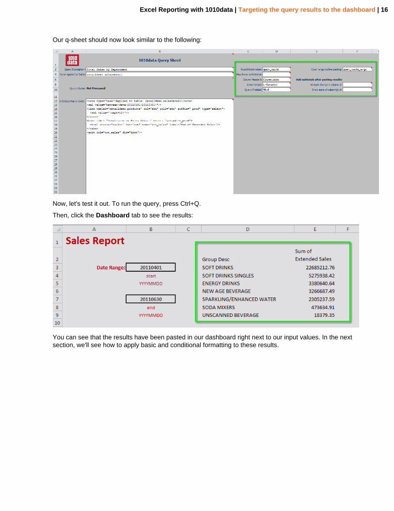
Our q-sheet should now look similar to the following:
Now, let's test it out. To run the query, press Ctrl+Q.
Then, click the Dashboard tab to see the results:
You can see that the results have been pasted in our dashboard right next to our input values. In the nextsection, we'll see how to apply basic and conditional formatting to these results.

Excel Reporting with 1010data | Formatting the results on the dashboard | 17
Formatting the results on the dashboard
You can apply basic and conditional formatting in Excel on the results that you got from running your1010data query.
Basic Formatting
Since this is a dashboard, we can add a little formatting to make it more visually appealing. So, for ourquery results, let's change the cells containing the column headers to be bold, and let's center the text inthose cells both horizontally and vertically.
We'll also change the format of the Sum of Extended Sales column to appear as dollar amounts. Right-click the column heading in Excel and click the $ from the context menu:
The values in that column will now be formatted correctly:

Excel Reporting with 1010data | Formatting the results on the dashboard | 18
These formats will be retained every time the query is run. We can verify that by changing the dates andrunning the query again. Change the start date to 20110701 (07/01/2011) and the end date to 20110930(09/30/2011). To run the query press Ctrl+Q (or click 1010data > Run Queries > In Active Workbook).When the query finishes running, you should see the following results:
You can see that the values in the Sum of Extended Sales column have changed to reflect the new daterange, and the formatting has been kept intact.
Conditional Formatting
We can also incorporate conditional formatting for the results from our 1010data query within our Excelworkbook. Let's say we want the format the range of values in the Sum of Extended Sales column using acolor scale. On the Home tab, click the Conditional Formatting button, and select Manage Rules... fromthe menu. The Conditional Formatting Rules Manager dialog is presented:

Excel Reporting with 1010data | Formatting the results on the dashboard | 19
Let's create a rule to apply conditional formatting using a color scale:
1. Click the New Rule... button.2. In the New Formatting Rule dialog, change the Format Style to 3-Color Scale, then click OK.3. In the Applies to field, enter =query_results_range, so that the rule will be applied to any of the
values that appear within the range we defined for our results earlier.4. Click Apply to create the new rule.
Let's also create a rule to show cells that have negative values with a red fill color:
1. Click the New Rule... button.2. From the Select a Rule Type list, select Format only cells that contain.3. Under Edit the Rule Description, make sure the first drop-down is Cell Value, change the second
drop-down to less than, and enter 0 in the third drop-down.4. Click the Format button.5. In the Format Cells dialog, click the Fill tab.6. Under Background Color, click the red box, then click OK.7. In the New Formatting Rule dialog, click OK .8. In the Conditional Formatting Rules Manager dialog, in the Applies to field, enter
=query_results_range.9. Click OK .
The results of our query are now formatted with a color scale:

Excel Reporting with 1010data | Formatting the results on the dashboard | 20
Our dashboard now shows us the total sales in a certain department within a specified date range andgroups those results by the values in the Group Desc column in the Product Master table. These resultsare also conditionally formatted using a color scale.
Let's add a simple chart to the dashboard to visually represent these results.
Excel Reporting with 1010data | Adding a simple chart to the dashboard | 21
Adding a simple chart to the dashboard
Leverage Excel's charting capabilities to visually represent the results from your query.
Let's combine Excel's easy-to-use charting functionality with the power and speed of running queries on1010data. Let's create a simple bar chart that shows the total sales for each group returned by our query.
We'll start by creating variables that will represent the x-axis and y-axis values for the chart.
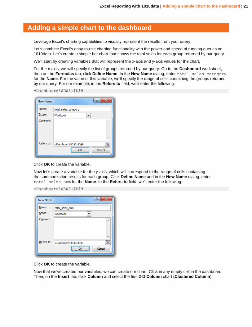
For the x-axis, we will specify the list of groups returned by our query. Go to the Dashboard worksheet,then on the Formulas tab, click Define Name. In the New Name dialog, enter total_sales_categoryfor the Name. For the value of this variable, we'll specify the range of cells containing the groups returnedby our query. For our example, in the Refers to field, we'll enter the following:
=Dashboard!$D$3:$D$9
Click OK to create the variable.
Now let's create a variable for the y-axis, which will correspond to the range of cells containingthe summarization results for each group. Click Define Name and in the New Name dialog, entertotal_sales_sum for the Name. In the Refers to field, we'll enter the following:
=Dashboard!$E$3:$E$9
Click OK to create the variable.
Now that we've created our variables, we can create our chart. Click in any empty cell in the dashboard.Then, on the Insert tab, click Column and select the first 2-D Column chart (Clustered Column):

Excel Reporting with 1010data | Adding a simple chart to the dashboard | 22
Position the chart where you want it to appear in the dashboard and resize it as desired:
Now let's incorporate the x-axis and y-axis variables we created earlier.
Let's start with the y-axis:
1. Right-click anywhere on the chart and click Select Data... from the context menu.2. In the Select Data Source dialog, click the Add button under Legend Entries (Series).
Excel Reporting with 1010data | Adding a simple chart to the dashboard | 23
3. In the Edit Series dialog, enter Total Sales for the Series name.4. In the Series values field, enter Dashboard!total_sales_sum, which is the name of the y-axis
variable we created earlier.5. Click OK.
And now, for the x-axis:
1. In the Select Data Source dialog, under Horizontal (Category) Axis Labels, click the Edit button.2. In the Axis Labels dialog, enter Dashboard!total_sales_category, which is the name of the x-
axis variable we created earlier.3. Click OK.
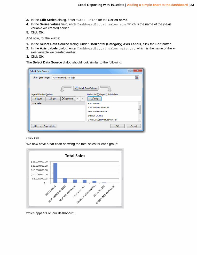
The Select Data Source dialog should look similar to the following:
Click OK.
We now have a bar chart showing the total sales for each group:
which appears on our dashboard:
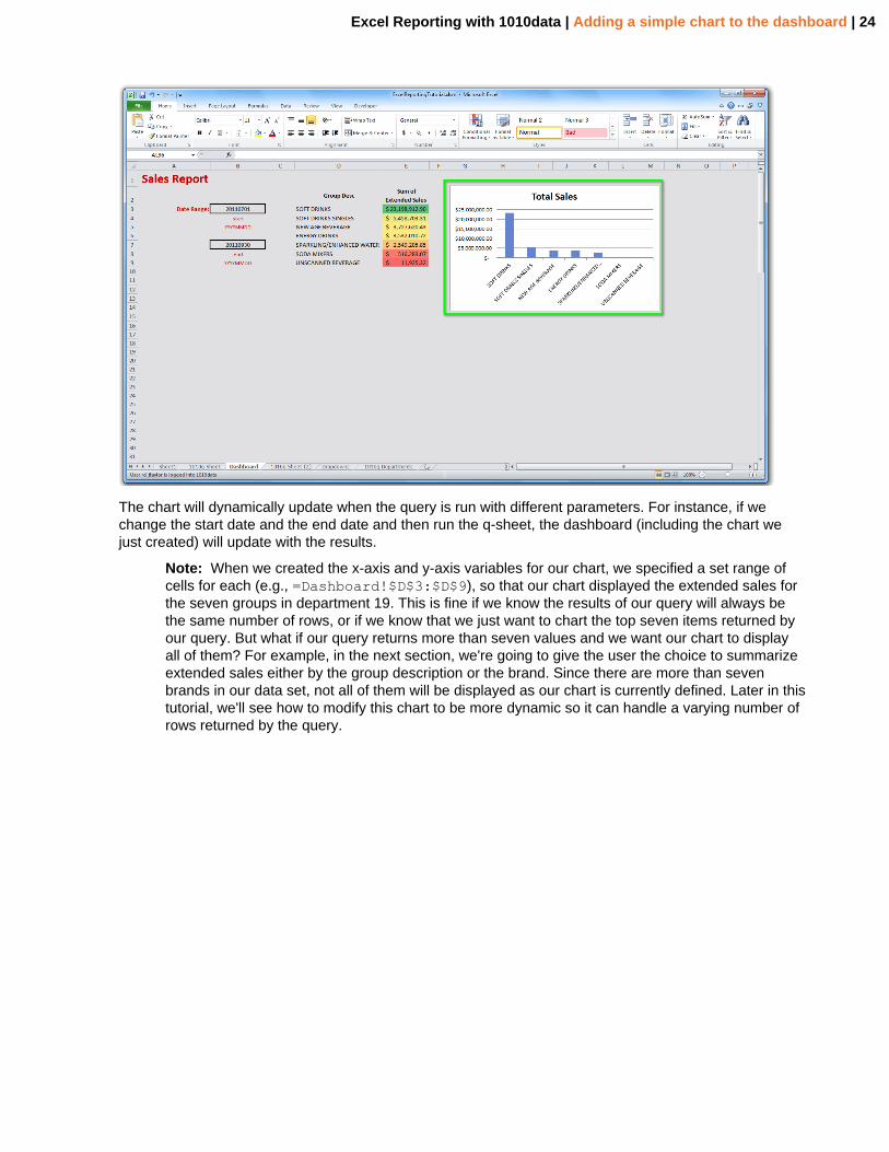
Excel Reporting with 1010data | Adding a simple chart to the dashboard | 24
The chart will dynamically update when the query is run with different parameters. For instance, if wechange the start date and the end date and then run the q-sheet, the dashboard (including the chart wejust created) will update with the results.
Note: When we created the x-axis and y-axis variables for our chart, we specified a set range ofcells for each (e.g., =Dashboard!$D$3:$D$9), so that our chart displayed the extended sales forthe seven groups in department 19. This is fine if we know the results of our query will always bethe same number of rows, or if we know that we just want to chart the top seven items returned byour query. But what if our query returns more than seven values and we want our chart to displayall of them? For example, in the next section, we're going to give the user the choice to summarizeextended sales either by the group description or the brand. Since there are more than sevenbrands in our data set, not all of them will be displayed as our chart is currently defined. Later in thistutorial, we'll see how to modify this chart to be more dynamic so it can handle a varying number ofrows returned by the query.

Excel Reporting with 1010data | Creating a static drop-down in the dashboard | 25
Creating a static drop-down in the dashboard
Let's create a drop-down to give the users of our dashboard the ability to select, from a static set of values,the column by which they want to group the results of the tabulation.
Currently, our query tabulates the sum of extended sales, grouping by the values in the Group Desccolumn in the Product Master table. Let's make it so that the user can select to group the results of thetabulation either by the group description or by the brand.
We're going to need a place to list the values that will populate the static drop-down. We can use Sheet3for our drop-down values (or create a new worksheet, if necessary). Let's rename it "Dropdowns".
In the Dropdowns worksheet, enter the following information:
Let's give this range of values a defined name. On the Formulas tab, click Define Name. In the NewName dialog, enter aggregate_by_values for the Name and enter the following for Refers to:=Dropdowns!$B$3:$B$4, then click OK.
Now let's go back to the Dashboard tab and create the static drop-down.
In the Dashboard worksheet, add the label "Aggregate by:" next to where you want the drop-down toappear.
Click the cell that you want to contain the drop-down. In our example, that would be cell B12. Let's givethat cell the defined name aggregate_by_dropdown.
From the Data tab, click Data Validation. In the Data Validation dialog, select List from the Allow drop-down, and enter =aggregate_by_values in the Source field:

Excel Reporting with 1010data | Creating a static drop-down in the dashboard | 26
Then click OK in the Data Validation dialog to finish creating the drop-down.
Now, if you click the newly created drop-down, you should see the two values, Group and Brand, in thelist:
Since we want the tabulation in our query to group by the item we select from the drop-down, we needto associate the choice in the drop-down with its corresponding column name. For instance, if someonechooses Brand from the drop-down, we want the query to specify the column brand_prod for thebreaks attribute to the <tabu> operation. Right now, it's hard-coded to be groupdesc_prod:
<note type="base">Applied to table: retaildemo.salesdetail</note><sel value="between(date;20110101;20110331)"/><link table2="retaildemo.products" col="sku" col2="sku" suffix="_prod" type="select"> <sel value="(dept=19)"/></link><tabu label="Tabulation on Sales Detail" breaks="groupdesc_prod"> <tcol source="xsales" fun="sum" name="tot_sales" label="Sum of`Extended Sales"/></tabu><sort col="tot_sales" dir="down"/>
So let's go back to the Dropdowns worksheet and add another column that will associate the drop-downchoices with their corresponding column names:

Excel Reporting with 1010data | Creating a static drop-down in the dashboard | 27
Since our query needs to reference a single cell (similar to what we did in Adding a static input to adashboard on page 12), we also need somewhere to store the choice that the user makes from the drop-down. Let's add one more column to the Dropdowns worksheet with a cell that will hold that value:
So, for our example, whatever choice the user selects from the drop-down will be stored in cell D3. Let'sgive that cell the defined name aggregate_by_selected
Let's add the functionality to populate that cell with the user's selection. We can use the Excel functionVLOOKUP() to help us do that. Let's add the following formula to cell D3:
=VLOOKUP(aggregate_by_dropdown,'Dropdowns'!B3:C4,2,FALSE)
This says that for the value in the aggregate_by_dropdown, search the first column in the table definedby the range 'Dropdowns'!B3:C4, and return the value in the second column (which we indicate bysetting the third parameter to 2), and only return if there is an exact match, which we specify by setting thelast parameter to FALSE Keep in mind that there will always be an exact match since we only have a finitenumber of defined choices in the drop-down.
So, if the user selects Brand from the drop-down in the Dashboard worksheet, the VLOOKUP functionwill search the values in the Drop-down Values column on the Dropdowns worksheet and will return thevalue in the second column, which is brand_prod:

Excel Reporting with 1010data | Creating a static drop-down in the dashboard | 28
Now that we have the column name, we can insert it into our query, just like we did in Adding a static inputto a dashboard on page 12.
The line that we need to change in our macro code is:
<note type="base">Applied to table: retaildemo.salesdetail</note><sel value="between(date;20110101;20110331)"/><link table2="retaildemo.products" col="sku" col2="sku" suffix="_prod" type="select"> <sel value="(dept=19)"/></link><tabu label="Tabulation on Sales Detail" breaks="groupdesc_prod"> <tcol source="xsales" fun="sum" name="tot_sales" label="Sum of`Extended Sales"/></tabu><sort col="tot_sales" dir="down"/>
To reference input values from within the 1010data query, we will need to change the line in our macrocode into a formula. We do this by:
• removing any blank spaces from the start of the line• inserting an = at the beginning of the line• enclosing the macro code in double quotes• preceding any double quote within the macro code with another double quote so that Excel will not
interpret any of them as the end of the formula• replacing each hard-coded value with a reference to its corresponding input cell using the syntax:
"&[CELL_REFERENCE]&" (e.g., "&B3&")
Let's go through those steps for our example. Click on the _1010q Sheet tab so that we can modify themacro code in our q-sheet.
Since there are no blank spaces at the start of the line, we can move to the next step and add an "=" to thebeginning:
=<tabu label="Tabulation on Sales Detail" breaks="groupdesc_prod">
Next, let's enclose the macro code in double quotes:
="<tabu label="Tabulation on Sales Detail" breaks="groupdesc_prod">"
Then, we'll precede each double quote within the macro code with another double quote so that Excel willnot interpret any of them as the end of the formula:
="<tabu label=""Tabulation on Sales Detail"" breaks=""groupdesc_prod"">"
Our last step is to replace the hard-coded groupdesc_prod value with a reference to theaggregate_by_selected cell, which contains the value the user selected from the drop-down:
="<tabu label=""Tabulation on Sales Detail"" breaks="""&aggregate_by_selected&""">"
Note: There are three sets of double quotes around &aggregate_by_selected&. Although thismay look odd, it is correct syntax for this Excel formula to work properly.
We can see the line in our macro code now consists of the formula we just created and that it resolves tobrand_prod within the 1010data Macro Code section of the q-sheet:
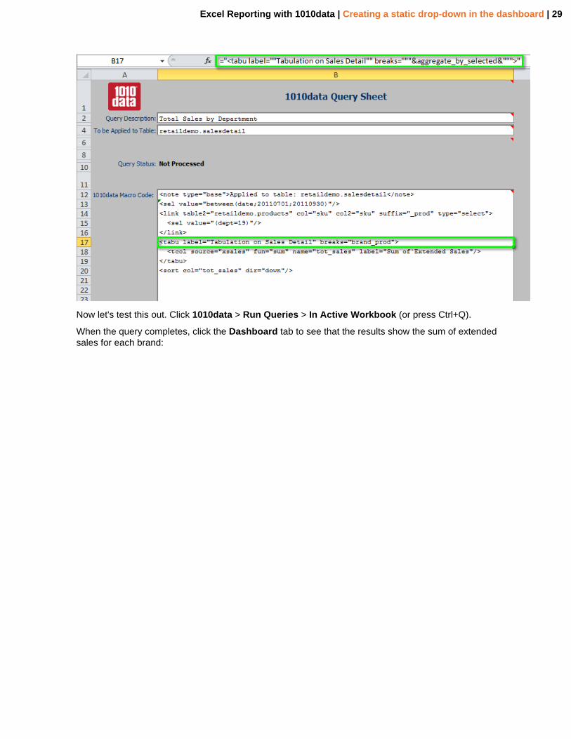
Excel Reporting with 1010data | Creating a static drop-down in the dashboard | 29
Now let's test this out. Click 1010data > Run Queries > In Active Workbook (or press Ctrl+Q).
When the query completes, click the Dashboard tab to see that the results show the sum of extendedsales for each brand:

Excel Reporting with 1010data | Creating a static drop-down in the dashboard | 30
The results we see are for department 19 only, since that was the department that was hard-coded in ouroriginal query. The next step will show how to add a dynamic drop-down that allows the user to choose anydepartment.
Excel Reporting with 1010data | Incorporating a dynamic drop-down in the dashboard | 31
Incorporating a dynamic drop-down in the dashboard
The contents of dynamic drop-downs can change based on selections in the dashboard or the resultsof queries, which means your dashboard will always be up to date even as the data changes. This ishistorically something very hard to do in Excel-based reporting and a big differentiator with using 1010dataand Excel.
Let's take a look at how to create a dynamic drop-down. Our original query calculated the sum of salesfor one particular department, which was hard-coded into the query. Let's say we want to give the user ofour dashboard the ability to select the department from a list of all the departments in our Product Mastertable. We could go through that table and list each department individually like we did in the previous step,Creating a static drop-down in the dashboard on page 25, but since our Product Master table has 59different departments, that would be a bit time consuming and could introduce errors (for instance, if adepartment number was entered incorrectly). It would be easier (and less susceptible to error) if we rana simple query on the Product Master table to find out the list of departments in the table and then usedthose results as the items in the drop-down. Let's create a dynamic drop-down to do just that.
We'll need to write a query that gives us a list of all the departments in the Product Master table, and we'llneed to put the results of that query in a place that our dashboard can access. We'll also need to createthe actual drop-down on the dashboard and populate it with the results of our department list query.
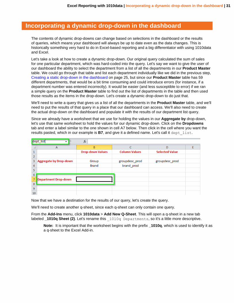
Since we already have a worksheet that we use for holding the values in our Aggregate by drop-down,let's use that same worksheet to hold the values for our dynamic drop-down. Click on the Dropdownstab and enter a label similar to the one shown in cell A7 below. Then click in the cell where you want theresults pasted, which in our example is B7, and give it a defined name. Let's call it dept_list.
Now that we have a destination for the results of our query, let's create the query.
We'll need to create another q-sheet, since each q-sheet can only contain one query.
From the Add-Ins menu, click 1010data > Add New Q-Sheet. This will open a q-sheet in a new tablabeled _1010q Sheet (2). Let's rename this _1010q Departments, so it's a little more descriptive.
Note: It is important that the worksheet begins with the prefix _1010q, which is used to identify it asa q-sheet to the Excel Add-in.
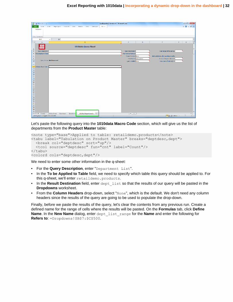
Excel Reporting with 1010data | Incorporating a dynamic drop-down in the dashboard | 32
Let's paste the following query into the 1010data Macro Code section, which will give us the list ofdepartments from the Product Master table:
<note type="base">Applied to table: retaildemo.products</note><tabu label="Tabulation on Product Master" breaks="deptdesc,dept"> <break col="deptdesc" sort="up"/> <tcol source="deptdesc" fun="cnt" label="Count"/></tabu><colord cols="deptdesc,dept"/>
We need to enter some other information in the q-sheet:
• For the Query Description, enter "Department List".• In the To be Applied to Table field, we need to specify which table this query should be applied to. For
this q-sheet, we'll enter retaildemo.products.• In the Result Destination field, enter dept_list so that the results of our query will be pasted in the
Dropdowns worksheet.• From the Column Headers drop-down, select "None", which is the default. We don't need any column
headers since the results of the query are going to be used to populate the drop-down.
Finally, before we paste the results of the query, let's clear the contents from any previous run. Create adefined name for the range of cells where the results will be pasted. On the Formulas tab, click DefineName. In the New Name dialog, enter dept_list_range for the Name and enter the following forRefers to: =Dropdowns!$B$7:$C$500.

Excel Reporting with 1010data | Incorporating a dynamic drop-down in the dashboard | 33
Note: This assumes that our result data will be less than 500 rows, which is probably safe for thisexample; however, you would want to specify a range that makes sense for you.
Then, in the _1010q Departments q-sheet, we can enter dept_list_range in the Clear range beforepasting field.
Our q-sheet should look similar to the following:
To run the q-sheet, click 1010data > Run Queries > In Active Workbook, or press Ctrl+Q.
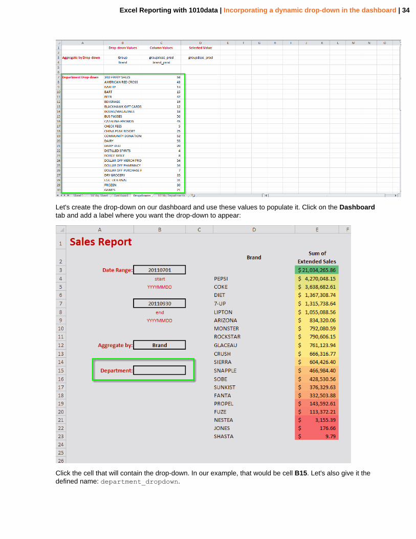
To see the results, click the Dropdowns tab. You can see that the results of the query have been pasted inthe cells that we specified:
Excel Reporting with 1010data | Incorporating a dynamic drop-down in the dashboard | 34
Let's create the drop-down on our dashboard and use these values to populate it. Click on the Dashboardtab and add a label where you want the drop-down to appear:
Click the cell that will contain the drop-down. In our example, that would be cell B15. Let's also give it thedefined name: department_dropdown.

Excel Reporting with 1010data | Incorporating a dynamic drop-down in the dashboard | 35
From the Data tab, click Data Validation. In the Data Validation dialog, select List from the Allow drop-down. For the Source field, you will need to use the following Excel OFFSET function:
=OFFSET(dept_list_range,0,0,COUNTA(dept_list_range),1)
The first parameter specifies the range of cells corresponding to the values in your query-generated drop-down list (which we named dept_list_range), and the second and third parameters tell the OFFSETfunction to start the list with the top left value in that range. The fourth parameter uses the Excel COUNTAfunction to calculate the number of non-empty cells in the range, which in essence specifies the length ofthe list. The last parameter tells the OFFSET function that we just want one column of data from the results.Dynamic drop-downs require this OFFSET function in conjunction with the COUNTA function to automaticallyaccount for the varying length of the list returned from our query. So, our Data Validation dialog will looksomething like:
Click OK in the Data Validation dialog to finish creating the drop-down.
Now, if you click the newly created drop-down, you should see the list of all the departments returned bythe query in the _1010q Departments q-sheet:

Excel Reporting with 1010data | Incorporating a dynamic drop-down in the dashboard | 36
Since we want our main query to perform the row selection based on the item we select from theDepartment drop-down, we need to associate the choice in the drop-down with its correspondingdepartment value. For instance, if someone chooses "DAIRY DELI" from the drop-down, we want thequery to specify department 20 in the value attribute to the <sel> operation. Right now, it's hard-codedto be 19:
<note type="base">Applied to table: retaildemo.salesdetail</note><sel value="between(date;20110101;20110331)"/><link table2="retaildemo.products" col="sku" col2="sku" suffix="_prod" type="select"> <sel value="(dept=19)"/></link><tabu label="Tabulation on Sales Detail" breaks="groupdesc_prod"> <tcol source="xsales" fun="sum" name="tot_sales" label="Sum of`Extended Sales"/></tabu><sort col="tot_sales" dir="down"/>
So let's go back to the Dropdowns worksheet and choose a cell that will contain the department valueassociated with the selected item in the Department drop-down (similar to what we did in Creating a staticdrop-down in the dashboard on page 25). For our example, we'll use cell D7. Let's give that cell the definedname department_selected.

Excel Reporting with 1010data | Incorporating a dynamic drop-down in the dashboard | 37
Let's add functionality to populate that cell with the department number that corresponds to the item theuser selects from the Department drop-down. We can use the Excel function VLOOKUP() to help us dothat. Let's add the following formula to cell D7:
=VLOOKUP(department_dropdown,dept_list_range,2,FALSE)
This says that for the value in the cell named department_dropdown, search the first column in the tabledefined by the range dept_list_range, and return the value in the second column, and only return ifthere is an exact match (which there will always be since we populated the drop-down from this list). So, ifthe user selects "DAIRY DELI" from the drop-down in the Dashboard worksheet, the VLOOKUP functionwill search the values in the Drop-down Values column on the Dropdowns worksheet until it finds amatch, and then return the value in the Column Values column, which for our example is 20:

Excel Reporting with 1010data | Incorporating a dynamic drop-down in the dashboard | 38
The last step is to reference the selected value in our original query. This process is essentially the sameas what we did in Adding a static input to a dashboard on page 12 and Creating a static drop-down in thedashboard on page 25.
The line that we need to change in our macro code is:
<note type="base">Applied to table: retaildemo.salesdetail</note><sel value="between(date;20110101;20110331)"/><link table2="retaildemo.products" col="sku" col2="sku" suffix="_prod" type="select"> <sel value="(dept=19)"/></link><tabu label="Tabulation on Sales Detail" breaks="groupdesc_prod"> <tcol source="xsales" fun="sum" name="tot_sales" label="Sum of`Extended Sales"/></tabu><sort col="tot_sales" dir="down"/>
To reference input values from within the 1010data query, we will need to change the line in our macrocode into a formula. We do this by:
• removing any blank spaces from the start of the line• inserting an = at the beginning of the line• enclosing the macro code in double quotes• preceding any double quote within the macro code with another double quote so that Excel will not
interpret any of them as the end of the formula• replacing each hard-coded value with a reference to its corresponding input cell using the syntax:
"&[CELL_REFERENCE]&" (e.g., "&B3&")
Let's go through those steps for our example. Click on the _1010q Sheet tab so that we can modify themacro code in our q-sheet.
First, remove any blank spaces from the start of the line:
<sel value="(dept=19)"/>
Then, add an "=" to the beginning of the line:
=<sel value="(dept=19)"/>

Excel Reporting with 1010data | Incorporating a dynamic drop-down in the dashboard | 39
Next, let's enclose the macro code in double quotes:
="<sel value="(dept=19)"/>"
Then, we'll precede each double quote within the macro code with another double quote so that Excel willnot interpret any of them as the end of the formula:
="<sel value=""(dept=19)""/>"
Our last step is to replace the hard-coded department 19 value with a reference to thedepartment_selected cell, which contains the value the user selected from the drop-down:
="<sel value=""(dept="&department_selected&")""/>"
Note: You must include the set of double quotes around &department_selected& for this Excelformula to work properly.
Now we can see the line in our macro code consists of the formula we just created and that it resolves to20 within the 1010data Macro Code section of the q-sheet:
Now let's test this out. Click 1010data > Run Queries > In Active Workbook (or press Ctrl+Q).
When the query completes, you can see that the results show the sum of extended sales for each brand indepartment 20:

Excel Reporting with 1010data | Incorporating a dynamic drop-down in the dashboard | 40
You can also see that the cell for the last item in the list, which contains a negative value, appears with adark red fill color, which we specified in Conditional Formatting on page 18.

Excel Reporting with 1010data | Adding another query to the dashboard | 41
Adding another query to the dashboard
In addition to aggregating total sales by either group description or brand for a specified department anddate range, we would also like to aggregate the total sales by date for the same department and daterange and display those results in our dashboard.
We have already created the framework to easily add this new query to our dashboard. Basically, we needto perform the following steps:
• Determine where on the dashboard we want our results to go• Create a new q-sheet for our new query and target the results to the dashboard
Determine the result destination on the dashboard
First let's figure out where we want our results to go. If we look at our dashboard, we can put our resultsright next to the other aggregation if we move our chart over to the right a bit:
Note: Since the first query will return results of varying length, it makes more sense to place theresults of the second query next to, not beneath, the first query in the dashboard.
Let's create a defined name for where the results of our query will be placed. On the Formulas tab, clickDefine Name. In the New Name dialog, enter query_2_results for the Name and enter the followingfor Refers to: =Dashboard!$G$2, then click OK.
Let's also create a defined name for the range to be cleared before pasting the results from a subsequentquery: Click Define Name. In the New Name dialog, enter query_2_results_range for the Name andenter the following for Refers to: =Dashboard!$G$2:$H$500, then click OK.
Note: This assumes that our result data will be less than 500 rows, which is probably safe for thisexample; however, you would want to specify a range that makes sense for you.
Create a new q-sheet
Now let's create a new q-sheet for the query we want to run on 1010data. From the Add-Ins menu, click1010data > Add New Q-Sheet. This will open a q-sheet in a new tab labeled _1010q Sheet (2).
We need to enter some other information in the q-sheet:
• For the Query Description, enter "Total Sales by Date".• In the To be Applied to Table field, enter retaildemo.salesdetail, since we want this query to be
applied to the same table as our first query.

Excel Reporting with 1010data | Adding another query to the dashboard | 42
• In the Result Destination field, enter query_2_results so that the results will be placed where wedecided on our dashboard.
• From the Column Headers drop-down, select "Column Labels".• In the Clear range before pasting field, we'll enter: query_2_results_range.
In the 1010data Macro Code box, enter the following Macro Language code:
<note type="base">Applied to table: retaildemo.salesdetail</note>="<sel value=""between(date;"&startdate&";"&enddate&")""/>"<note type="link">The following link is to table: All Databases/Retail Demo Data/Product Master</note><link table2="retaildemo.products" col="sku" col2="sku" type="select" suffix="_prod">="<sel value=""(dept="&department_selected&")""/>"</link><willbe name="date_formatted" value="date" format="type:date" label="Date"/><tabu label="Tabulation on Sales Detail" breaks="date_formatted"> <break col="date_formatted" sort="up"/> <tcol source="xsales" fun="sum" name="tot_sales" label="Sum of`Extended`Sales"/></tabu>
Note: The lines in bold are Excel formulas that reference the start and end dates (startdate andenddate) as well as the department number (department_selected) that the user provideson the dashboard. (See Adding a static input to a dashboard on page 12 and Creating a staticdrop-down in the dashboard on page 25 for more details on how to reference input values within1010data Macro Language code.)
Our new q-sheet should look similar to the following:
Note: The lines containing the Excel formulas display the values of the cells that theyare referencing. For example, department number 20 appears for the reference todepartment_selected in cell B16 within the 1010data Macro Code section.
Now let's test this out. Click 1010data > Run Queries > In Active Workbook (or press Ctrl+Q).
You can see the results from both queries next to one another in the dashboard:

Excel Reporting with 1010data | Adding another query to the dashboard | 43
Note: You can format the column headings and the dollar amounts, which appear in the newSum of Extended Sales column, so that the look across the dashboard is consistent. (See BasicFormatting on page 17 for details.)
It would be even more convenient if we could run the queries directly from our dashboard. The next stepwill show how to add a button to the dashboard that will allow you to do just that.

Excel Reporting with 1010data | Adding a button to run the queries | 44
Adding a button to run the queries
We want to be able to run our queries by simply clicking a button on the dashboard.
Click on the Dashboard tab. Let's add the button somewhere around cell B18 on that worksheet:
On the Developer tab, click the Insert button to bring up the Form Controls and then click the icon in thetop left corner, which corresponds to the Button (Form Control).
Note: If the Developer tab does not appear in your ribbon, click File > Options > CustomizeRibbon. Under the Customize the Ribbon list on the right side of the dialog, select Developer andthen click OK. The Developer tab should now appear in the ribbon.
Excel Reporting with 1010data | Adding a button to run the queries | 45
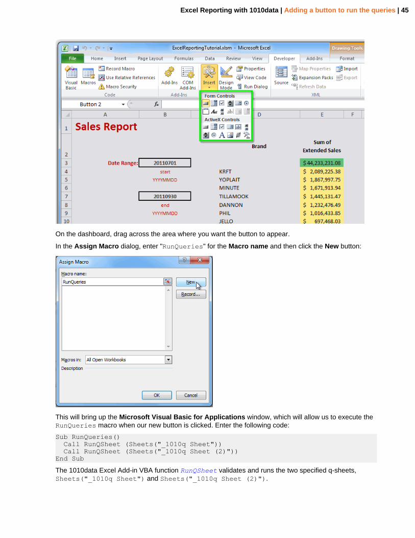
On the dashboard, drag across the area where you want the button to appear.
In the Assign Macro dialog, enter "RunQueries" for the Macro name and then click the New button:
This will bring up the Microsoft Visual Basic for Applications window, which will allow us to execute theRunQueries macro when our new button is clicked. Enter the following code:
Sub RunQueries() Call RunQSheet (Sheets("_1010q Sheet")) Call RunQSheet (Sheets("_1010q Sheet (2)"))End Sub
The 1010data Excel Add-in VBA function RunQSheet validates and runs the two specified q-sheets,Sheets("_1010q Sheet") and Sheets("_1010q Sheet (2)").

Excel Reporting with 1010data | Adding a button to run the queries | 46
Note: If you don't want the status bar to appear while queries are being run, or if you arerunning several q-sheets and don't want to click OK after each one completes, you can add theparameter Quiet:=True to the RunQSheet function calls. For example, Call RunQSheet(Sheets("_1010q Sheet"), Quiet:=True)
Let's make sure our VBA project has a reference to the 1010data Excel Add-in VBA library. In theMicrosoft Visual Basic for Applications window, click Tools > References and select A1010data fromthe list of Available References, if it is not already selected.
Click OK, then save the macro by pressing Ctrl+S.
After you close the Microsoft Visual Basic for Applications window, you should see the new button onthe dashboard:

Excel Reporting with 1010data | Adding a button to run the queries | 47
Change the text of the button to "RUN" and change the font size and style as you like. When you're done,right-click the new button and click Exit Edit Text from the context menu.
Now we're ready to test out our new button. Let's modify the date range once again so that we can seeif the sales totals update. Let's change the start date to 20111001 and the end date to 20111231. Thenclick the RUN button.
Note: After each query completes, you will be presented with a dialog that you must dismiss beforethe next query runs.
When the queries complete, we can see the results on the dashboard.

Excel Reporting with 1010data | Adding a button to run the queries | 48
You will notice that the chart has also been updated. However, it only shows the top seven items returnedfrom our first query. Let's modify the chart so that it will dynamically include all of the items returned fromthe first query. We'll also add a second chart that shows the results of the query that aggregates total salesby date.

Excel Reporting with 1010data | Charting the results dynamically on the dashboard | 49
Charting the results dynamically on the dashboard
Utilize more advanced charting techniques in Excel to show the details in the results returned by our1010data queries.
Here's what our dashboard looks like up to this point:
Our chart only shows the top seven items returned from our first query. Let's modify the chart so that it willdynamically include all of the items returned from the first query. We'll also add a line chart for the resultsof the second query to show the total sales by date for the same department.
Making the bar chart more dynamic
Our first query returns the total sales for each group or brand in a specific department. The bar chart wecreated earlier only shows the top seven items returned by the query, because we hard-coded a range ofvalues for the x-axis and y-axis variables. Let's modify those variables, so that our chart will dynamicallydisplay all of the items returned by the query.
On the Formulas tab, click the Name Manager button. In the Name Manager dialog, click thetotal_sales_category item in the list, and then click the Edit... button. For the value of this variable,we're going to use the Excel OFFSET function. In the Refers to field in the Edit Name dialog, we'll enterthe following:
=OFFSET(query_results,1,0,COUNTA(Dashboard!$D:$D),1)
The first parameter specifies the cell from which you want to base the offset, so we'll specifyquery_results for that parameter. The list of groups or brands returned from our first query begins atone row below in the same column as the cell named query_results, so we'll specify 1 for the secondparameter to indicate one row below, and we'll specify 0 for the third parameter to indicate the samecolumn. The fourth parameter uses the Excel COUNTA function to calculate the number of non-empty cellsin column D, because all information charted has to correspond to a value along the x-axis, and thosevalues are in column D. The last parameter tells the OFFSET function that we just want one column of datafrom the results.

Excel Reporting with 1010data | Charting the results dynamically on the dashboard | 50
Click OK to modify the variable.
Now let's modify the y-axis variable. In the Name Manager dialog, click the total_sales_sum item inthe list, and then click the Edit... button. In the Refers to field in the Edit Name dialog, we'll enter thefollowing:
=OFFSET(query_results,1,1,COUNTA(Dashboard!$D:$D),1)
For the first parameter, we specify query_results like we did for the x-axis variable. The list of totalsales returned from our first query begins at one row below and one column to the right of the cell namedquery_results, so we'll specify 1 for the second parameter to indicate one row below, and we'llspecify 1 for the third parameter to indicate one column to the right. For the fourth parameter, we'll usethe Excel COUNTA function again to calculate the number of non-empty cells in column D, because allinformation charted has to correspond to a value along the x-axis, and those values are in column D. Thelast parameter tells the OFFSET function that we just want one column of data from the results.
Click OK to modify the variable.
In the Name Manager dialog, click Close.
The chart will automatically update to show all of the items returned from our query:

Excel Reporting with 1010data | Charting the results dynamically on the dashboard | 51
Note: You may want to resize the chart to accommodate the additional items along the x-axis.
Creating a line chart
We can also create a line chart that shows the results from our second query, so that we can see totalsales by date for the department we have selected.
Once again, we need to create variables that will represent the x-axis and y-axis values for the chart. Forthe x-axis, we will specify the list of dates returned by our query. The determination of their values followsthe same logic as the variables we created for the bar chart in the previous section, so we won't go into asdetailed an explanation here.
On the Formulas tab, click Define Name. In the New Name dialog, enter daily_sales_date for theName. In the Refers to field, we'll enter the following:
=OFFSET(query_2_results,1,0,COUNTA(Dashboard!$G:$G),1)
Click OK to create the variable.
Now let's create a variable for the y-axis. Click Define Name and in the New Name dialog, enterdaily_sales_sum for the Name. In the Refers to field, enter the following:
=OFFSET(query_2_results,1,1,COUNTA(Dashboard!$G:$G),1)

Excel Reporting with 1010data | Charting the results dynamically on the dashboard | 52
Click OK to create the variable.
Now that we've created our variables, we can create our chart. Click in any empty cell in the dashboard.Then, on the Insert tab, click Line and select the first 2-D Line chart (Line):
Position the chart where you want it to appear in the dashboard and resize it as desired:
Excel Reporting with 1010data | Charting the results dynamically on the dashboard | 53
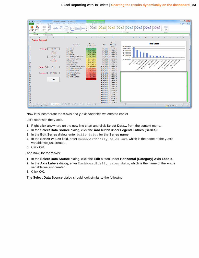
Now let's incorporate the x-axis and y-axis variables we created earlier.
Let's start with the y-axis.
1. Right-click anywhere on the new line chart and click Select Data... from the context menu.2. In the Select Data Source dialog, click the Add button under Legend Entries (Series).3. In the Edit Series dialog, enter Daily Sales for the Series name.4. In the Series values field, enter Dashboard!daily_sales_sum, which is the name of the y-axis
variable we just created.5. Click OK.
And now, for the x-axis:
1. In the Select Data Source dialog, click the Edit button under Horizontal (Category) Axis Labels.2. In the Axis Labels dialog, enter Dashboard!daily_sales_date, which is the name of the x-axis
variable we just created.3. Click OK.
The Select Data Source dialog should look similar to the following:

Excel Reporting with 1010data | Charting the results dynamically on the dashboard | 54
Click OK.
We now have a line chart showing the total sales by date for the department we've selected:
which appears on our dashboard:
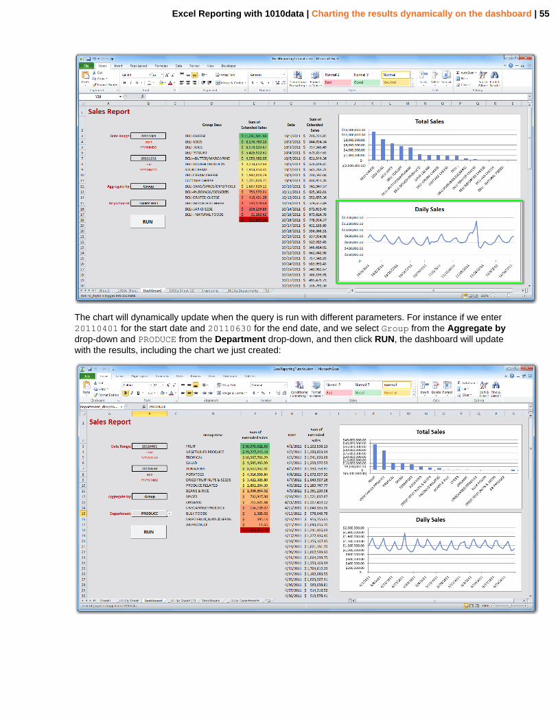
Excel Reporting with 1010data | Charting the results dynamically on the dashboard | 55
The chart will dynamically update when the query is run with different parameters. For instance if we enter20110401 for the start date and 20110630 for the end date, and we select Group from the Aggregate bydrop-down and PRODUCE from the Department drop-down, and then click RUN, the dashboard will updatewith the results, including the chart we just created:

Excel Reporting with 1010data | Using 1010data libraries and blocks | 56
Using 1010data libraries and blocks
You can make the Excel Add-in even more dynamic by accessing query code in libraries and blocks on1010data.
One of the most powerful features of 1010data is the use of libraries and blocks to encapsulate MacroLanguage code. Libraries consist of one or more blocks, each of which contains Macro Language codethat can be inserted within other queries. This allows you to keep your query code in a central location andgive multiple users access to it. If you need to change the code for any reason (e.g., one of the calculationsneeds to change), you can simply change the block. Whenever anybody inserts the block into their query,they will get the most up-to-date code.
To see how this works, we'll log into the 1010data web interface to create a library. The library will consistof one block that contains the code for the second query on our dashboard. As you'll recall, this querycalculates the total sales by date for a given department.
Note: If you are not already logged into the 1010data web interface, when you attempt to log in,you will see a message prompting you to either re-enter or end your existing session. You mustselect End existing session, which will log you out of your Excel Add-in session. Consequently,you will need to log in via the Excel Add-in again before you can run your q-sheets.
Our <library>, which consists of a <block> named sales_by_date, would look something like thefollowing:
<note type="base">Applied to table: retaildemo.salesdetail</note><library> <block name="sales_by_date" start="20110101" end="20110331" department="19"> <sel value="between(date;{@start};{@end})"/> <note type="link">The following link is to table: All Databases/Retail Demo Data/Product Master</note> <link table2="retaildemo.products" col="sku" col2="sku" type="select" suffix="_prod"> <sel value="(dept={@department})"/> </link> <willbe name="date_formatted" value="date" format="type:date" label="Date"/> <tabu label="Tabulation on Sales Detail" breaks="date_formatted"> <break col="date_formatted" sort="up"/> <tcol source="xsales" fun="sum" name="tot_sales" label="Sum of`Extended`Sales"/> </tabu> </block></library>
You'll notice that the code within the <block> is almost identical to the code that we used in Addinganother query to the dashboard on page 41.
You'll also notice that the <block> takes three parameters: start, end, and department. Theparameters are then referenced in the query using the {@PARAM_NAME} syntax (e.g., {@start}).
Note: We specify default values for these parameters in the <block> definition (e.g.,start="20110101").
The library is then saved as a Quick Query in a folder on 1010data.
Note: Users who want to use any of the blocks in the library must be given the appropriatepermissions to the requisite folders and tables. See How to Share Quick Queries and Folders in theQuick Start Guide for more information.
For this example, let's say that the path to the Quick Query containing this library is:uploads.t632564076_rd_jtaylor.
Excel Reporting with 1010data | Using 1010data libraries and blocks | 57
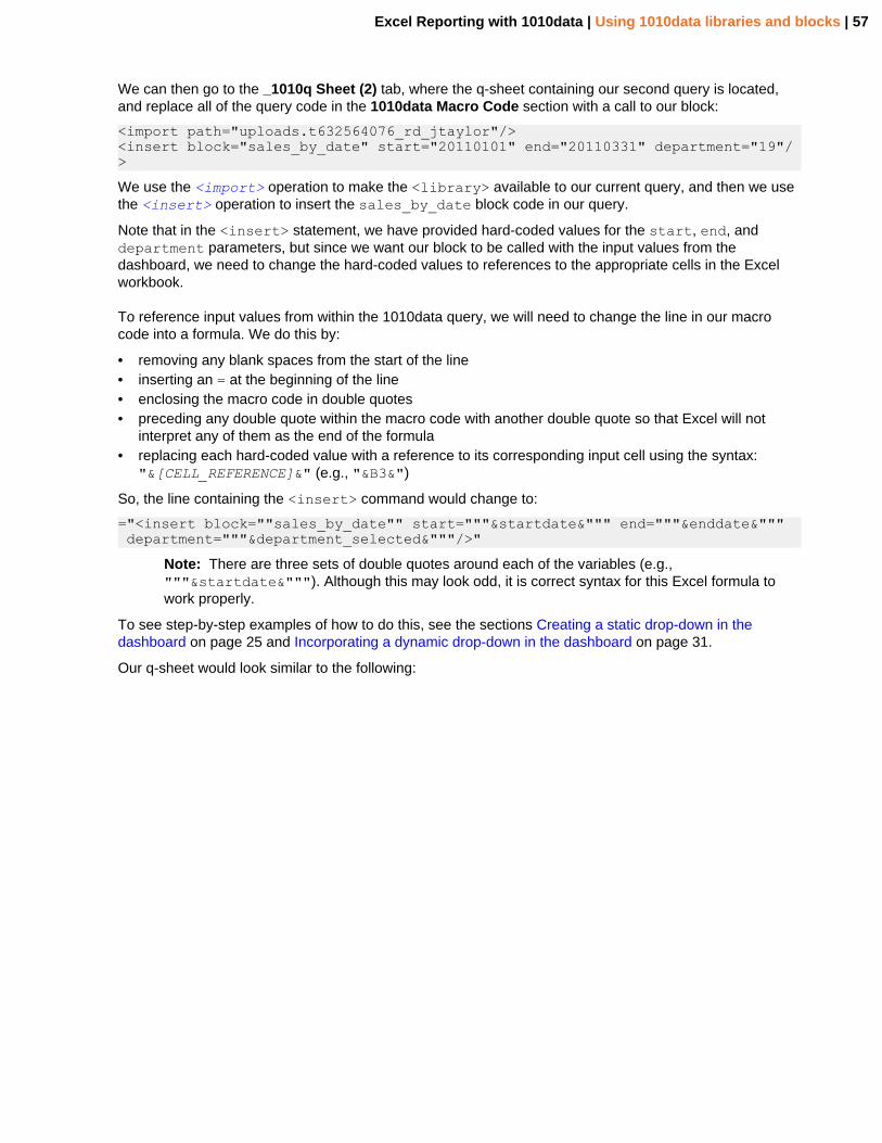
We can then go to the _1010q Sheet (2) tab, where the q-sheet containing our second query is located,and replace all of the query code in the 1010data Macro Code section with a call to our block:
<import path="uploads.t632564076_rd_jtaylor"/><insert block="sales_by_date" start="20110101" end="20110331" department="19"/>
We use the <import> operation to make the <library> available to our current query, and then we usethe <insert> operation to insert the sales_by_date block code in our query.
Note that in the <insert> statement, we have provided hard-coded values for the start, end, anddepartment parameters, but since we want our block to be called with the input values from thedashboard, we need to change the hard-coded values to references to the appropriate cells in the Excelworkbook.
To reference input values from within the 1010data query, we will need to change the line in our macrocode into a formula. We do this by:
• removing any blank spaces from the start of the line• inserting an = at the beginning of the line• enclosing the macro code in double quotes• preceding any double quote within the macro code with another double quote so that Excel will not
interpret any of them as the end of the formula• replacing each hard-coded value with a reference to its corresponding input cell using the syntax:
"&[CELL_REFERENCE]&" (e.g., "&B3&")
So, the line containing the <insert> command would change to:
="<insert block=""sales_by_date"" start="""&startdate&""" end="""&enddate&""" department="""&department_selected&"""/>"
Note: There are three sets of double quotes around each of the variables (e.g.,"""&startdate&"""). Although this may look odd, it is correct syntax for this Excel formula towork properly.
To see step-by-step examples of how to do this, see the sections Creating a static drop-down in thedashboard on page 25 and Incorporating a dynamic drop-down in the dashboard on page 31.
Our q-sheet would look similar to the following:

Excel Reporting with 1010data | Using 1010data libraries and blocks | 58
You can see in the 1010data Macro Code section that the actual values corresponding to the start, end,and department_selected inputs on our dashboard appear in the code:
If we change the values on the dashboard:
The values in our <insert> call in the q-sheet will change as well:

Excel Reporting with 1010data | Using 1010data libraries and blocks | 59
Note: Before you run the q-sheets, you may have to log in once again. From the Add-Ins tab, click1010data > 1010data Login..., enter your credentials, and then click Secure Login.
Now, if we go to the dashboard and click the RUN button, the second query will run the code from our<block>, and the dashboard will update accordingly:
Libraries and blocks give you flexibility in providing your users with the most up-to-date query code. In thisway, you can provide templates to your business users and change metric calculations without needingto update or send new Excel templates. If something within the block changes, the Excel Add-in willautomatically leverage the new definition going forward.

Excel Reporting with 1010data | Hiding worksheets and locking the workbook | 60
Hiding worksheets and locking the workbook
If you are planning to share your workbook with other users, you may want to hide all q-sheets and lock theworkbook to prevent accidental edits to your query code.
Hiding worksheets
Because our dashboard is self-contained, there is no need for users to see or access the q-sheets or, forthat matter, the Dropdowns worksheet we used to hold the values for the drop-downs in our dashboard. Itis also a good idea to hide q-sheets to prevent the user from changing the query code.
You can hide a worksheet by right-clicking its tab and then selecting Hide from the context menu:
For our example, we would hide the following worksheets:
• _1010q Sheet• _1010q Sheet (2)• _1010q Departments• Dropdowns• Sheet1
Note: In fact, you could delete Sheet1 since it is no longer needed.
Once those worksheets are hidden, our workbook looks like:

Excel Reporting with 1010data | Hiding worksheets and locking the workbook | 61
To unhide worksheets you have previously hidden, right-click anywhere along your worksheets pane at thebottom of your workbook and click Unhide. From the Unhide dialog, you can select which worksheets youwould like to be visible again:
Locking the workbook
To prevent users from unhiding worksheets, you can lock the workbook. On the Review tab, click ProtectWorkbook:
In the Protect Structure and Windows dialog, make sure that Structure is selected:

Excel Reporting with 1010data | Hiding worksheets and locking the workbook | 62
If you want to require the user to provide a password to unhide worksheets, enter a password in thePassword (optional) field.
Click OK for the changes to take effect.
Note: Once the workbook has been locked, you need to click Protect Workbook on the Reviewtab to be able to make changes to the workbook. If a password is required, you must enter thepassword in the Unprotect Workbook dialog and click OK
Now your dashboard is ready to send out to others!


