arXiv:0912.1612v1 [hep-th] 8 Dec 2009 Exceptional Lie algebras and M-theory Jakob Palmkvist Physique Th´ eorique et Math´ ematique Universit´ e Libre de Bruxelles & International Solvay Institutes Boulevard du Triomphe, Campus Plaine, ULB-CP 231, BE-1050 Bruxelles, Belgium [email protected]Thesis for the degree of Doctor of Philosophy, defended on December 10, 2008, at Fundamental Physics, Chalmers University of Technology, G¨ oteborg, Sweden. The work was funded by the International Max Planck Research School for Geometric Analysis, Gravitation and String Theory, and conducted at the Max Planck Institute for Gravitational Physics (Albert Einstein Institute) in Potsdam, Germany. Abstract In this thesis we study algebraic structures in M-theory, in particular the exceptional Lie algebras arising in dimensional reduction of its low energy limit, eleven-dimensional supergravity. We focus on e 8 and its infinite-dimensional extensions e 9 and e 10 . We review the dynamical equivalence, up to truncations on both sides, between eleven- dimensional supergravity and a geodesic sigma model based on the coset E 10 /K (E 10 ), where K (E 10 ) is the maximal compact subgroup. The description of e 10 as a graded Lie algebra is crucial for this equivalence. We study generalized Jordan triple systems, which are closely related to graded Lie algebras, and which may also play a role in the description of M2-branes using three-dimensional superconformal theories.
Transcript
arX
iv:0
912.
1612
v1 [
hep-
th]
8 D
ec 2
009
Exceptional Lie algebras
and M-theory
Jakob Palmkvist
Physique Theorique et MathematiqueUniversite Libre de Bruxelles & International Solvay Institutes
Boulevard du Triomphe, Campus Plaine, ULB-CP 231,BE-1050 Bruxelles, Belgium
Thesis for the degree of Doctor of Philosophy, defended on December 10, 2008,at Fundamental Physics, Chalmers University of Technology, Goteborg, Sweden.
The work was funded by the International Max Planck Research School for GeometricAnalysis, Gravitation and String Theory, and conducted at the Max Planck Institute
for Gravitational Physics (Albert Einstein Institute) in Potsdam, Germany.
Abstract
In this thesis we study algebraic structures in M-theory, in particular the exceptionalLie algebras arising in dimensional reduction of its low energy limit, eleven-dimensionalsupergravity. We focus on e8 and its infinite-dimensional extensions e9 and e10. Wereview the dynamical equivalence, up to truncations on both sides, between eleven-dimensional supergravity and a geodesic sigma model based on the coset E10/K(E10),where K(E10) is the maximal compact subgroup. The description of e10 as a gradedLie algebra is crucial for this equivalence. We study generalized Jordan triple systems,which are closely related to graded Lie algebras, and which may also play a role in thedescription of M2-branes using three-dimensional superconformal theories.
First of all, I would like to thank Professor Hermann Nicolai, not only in his role asmy supervisor, but also as a director of the Albert Einstein Institute, where I have hadthe pleasure to work the last three years. I am also grateful to my official supervisorProfessor Martin Cederwall and my examiner Professor Bengt E. W. Nilsson. Further-more, I would like to thank Axel Kleinschmidt and our collaborators in Groningen:Eric A. Bergshoeff, Olaf Hohm and Teake A. Nutma, especially for their efforts tofinish one of the papers when the deadline for my thesis was approaching. I am grate-ful to Jonas Hartwig, Ling Bao and especially Daniel Persson for carefully readingparts of the manuscript and giving me many valuable comments. I am also gratefulto Christoffer Petersson for generously lending me his sofa and his office during myvisits in Goteborg. Finally, among the students and postdocs at the Albert EinsteinInstitute I would especially like to thank Sudarshan Ananth, Claudia Colonnello, Ce-cilia Flori, Thomas Klose, Michael Koehn, Carlo Meneghelli and Hidehiko Shimada fortheir support and friendship.
There are four fundamental forces in nature. Three of them, the electromagnetic, weakand strong interactions, can be described within the framework of quantum mechanics.The fourth force, gravity, is one that we all experience every day, but it is also the leastunderstood of the four forces. Einstein’s theory of general relativity works well in mostsituations, and it is already a great improvement of Newton’s theory. However, at highenergies and small distances, for example near the center of a black hole or shortlyafter the big bang, we need a quantum theory to describe gravity. In particular, thisimplies the existence of a spin two particle, called the graviton, mediating the force.
String theory was originally developed in the late 1960s as a theory of strong in-teraction, which keeps the quarks together within the hadrons. However, anotherdescription of strong interaction, called quantum chromodynamics (QCD) appeared inthe early 1970s and turned out to be more successful. One of the drawbacks of stringtheory in this context is the existence of a spin two particle, which has no hadronicinterpretation. However, this also has the advantage that string theory may, and in-deed has to, be interpreted as a theory of quantum gravity. On the other hand, thespectrum of the bosonic string theory contains a tachyon, a state with negative masssquared. One can get rid of this problem by imposing supersymmetry and consideringsuperstrings instead of bosonic strings. Supersymmetry is a symmetry between bosons(particles that mediate forces) and fermions (particles that build up matter). Althoughnot yet experimentally observed, supersymmetry is a very natural property to requirefor a theory of all known forces and matter, since it implies that the strengths of theelectromagnetic, weak and strong interactions coincide at a certain energy scale.
A problem of bosonic string theory that cannot be solved by supersymmetry is the(natural) appearance of extra dimensions. Bosonic string theory does not work in thefour-dimensional world that we live in, but requires 26 dimensions. Supersymmetryreduces this number, but only down to 10. One way to come around this obstacle isto think of some of the dimensions as closed circles instead of lines that are infinitely
1
extended in both directions. If all except four of these circles are sufficiently small,they cannot be distinguished from points and the theory is effectively four-dimensional.This is an example of compactification – all but four of the dimensions are compact. Ifwe compactify n dimensions, each spacetime point in the effective lower-dimensionaltheory can be interpreted as an n-dimensional manifold. In the example with a circlefor each compact dimension, the resulting manifold is an n-torus, but there are othermuch more complicated possibilities. Compactification can be seen as a source ofunification – seemingly unrelated features of a theory can have a common origin in ahigher-dimensional theory, compactified on an appropriate manifold.
In the first superstring revolution 1984–85 two new string theories in ten dimensionswere found, called heterotic string theories, with SO(32) and E8×E8 as gauge groups,respectively. It was shown by Green and Schwarz that for these groups (but no others)all anomalies cancel [1,2]. Moreover, upon compactification on a so called Calabi-Yaumanifold the E8 × E8 theory may lead to the gauge group U(1) × SU(2) × SU(3)that describes the electromagnetic, weak and strong interactions. In addition to theheterotic theories, there were already two theories of closed strings, called type IIA andtype IIB, and a fifth theory, called type I, with both open and closed strings.
The fact that string theory on the one hand exhibited promising features as a the-ory of quantum gravity, and on the other hand required supersymmetry and extradimensions, raised the interest in supergravity in various dimensions, and with variousamount of supersymmetry. It was shown that eleven is the maximal number of di-mensions for a supergravity theory with Minkowski signature and without particles ofhigher spin than two [3]. Furthermore, in eleven dimensions there is only one supergrav-ity theory [4], whereas there are more possibilities in lower dimensions. Dimensionalreduction of eleven-dimensional supergravity on a circle gives type IIA supergravity,which is the low energy limit of type IIA string theory. More generally, reduction onan n-torus, gives maximal supergravity in 11− n dimensions.
In the second superstring theory revolution 1994–95, Hull, Townsend [5] and Witten[6] showed that the five string theories are connected by dualities. It was proposed thateleven-dimensional supergravity is the low energy limit of a more fundamental theory,called M-theory. Unlike strings, the fundamental objects in M-theory are believedto be extended in not only one but two spatial directions. Such objects are calledsupermembranes or M2-branes. Very little is known about M-theory but we can learnmore about it by studying its low energy limit, eleven-dimensional supergravity, andits reductions.
Toroidal reduction of eleven-dimensional supergravity to d = 11 − n dimensionsgives rise to symmetries in the reduced theories, which are said to be hidden sincesome of the fields must be dualized to make the symmetry manifest. After dualizationthe scalars in the d-dimensional theory parameterize the coset G/K(G), where G is theglobal symmetry group of the Lagrangian, and K(G) is its maximal compact subgroup(which appears as a local symmetry). For 4 ≤ n ≤ 8, the symmetry groups G are theexceptional groups En, with Lie algebras en [7–9].
2
In three dimensions all the bosonic degrees of freedom can be dualized to scalars andcan thereby be described by a sigma model based on the coset E8/(Spin(16)/Z2) [10,11].The fact that scalars are dual to scalars in two dimensions makes the step from d = 3down to d = 2 different from the preceding steps in the successive reduction. Thecorresponding E9 and K(E9) symmetries are not realized on the action but on theequations of motion, which can be written as an integrability condition of a linearsystem [12]. This difference is on the mathematical side reflected by the fact that e9 isinfinite-dimensional, unlike en for 4 ≤ n ≤ 8. The appearance of infinite-dimensionalsymmetries in d = 2 was first studied by Geroch for pure gravity reduced from four totwo dimensions [13, 14].
One might suspect that e10 should appear in the reduction to only one (time)dimension, or even e11 in zero dimensions [15, 16]. Partial results concerning e10 werefound in [17]. Although e9 and e10 both are infinite-dimensional and both can bedefined recursively, there is a crucial difference in complexity. For e9, which is an affinealgebra, there is a pattern that repeats itself and makes it possible to write down allthe commutation relations in a closed form. For e10, a hyperbolic algebra, the numberof new elements grows exponentially for each step in the recursive definition, and soonone looses control over the algebra.
Beside the conjectural symmetry in the reduction to one dimension, hyperbolic Kac-Moody algebras were also shown to appear near spacelike singularities in supergravitytheories [18, 19]. The chaotic behavior in this limit [20] can be reformulated as abilliard motion in the Weyl chamber of a hyperbolic Kac-Moody algebra, which foreleven-dimensional supergravity is e10.
Inspired by the coset symmetries in dimensional reduction and the appearance ofhyperbolic algebras in cosmological billiards, Damour, Henneaux and Nicolai consid-ered a one-dimensional geodesic sigma model based on the infinite-dimensional cosetE10/K(E10) [21]. They found a correspondence, up to truncations on both sides,between the sigma model equations of motion and those of eleven-dimensional super-gravity at a fixed, but arbitrarily chosen spatial point [21, 22]. Corresponding resultsfor the maximal supergravity theories in ten dimensions were obtained in [23,24] usingthe same coset model, but different level decompositions. The model has also beenextended to the fermionic sector of eleven-dimensional supergravity, involving spinorand vector-spinor representations of k(e10) [25–28]. These representations are finite-dimensional and thus unfaithful, since the algebra itself is infinite-dimensional. Thereare problems with the model related to this fact, and the construction of a faithfulfermionic representation would probably be an important progress. In an alterna-tive approach it has been has been proposed that eleven-dimensional supergravity isa nonlinear realization of the Lorentzian algebra e11 [29]. See also [30, 31] for a modelcombining the approaches in [21] and [29].
3
1.1 Outline
This text consists of six chapters and is intended to be an introduction to the fiveresearch papers [32–36].
In chapter 2 we review how dimensional reduction gives rise to coset symmetries.We do this in detail for pure gravity in D dimensions reduced to d = D−n dimensions.We also discuss very briefly how the symmetry gets enhanced from GL(n) to SL(n+1)in d = 3. Taking all the bosonic fields in supergravity into account, the global symmetrygroups are extended to (the split real forms of) the exceptional groups En for 4 ≤ n ≤ 8.In order to describe the corresponding Lie algebras, in particular for E8 and its infinite-dimensional extensions E9 and E10, we need the mathematical background presented inchapter 3 and 4. The first of these chapters provides the standard classification of Kac-Moody algebras, including also the simple finite-dimensional Lie algebras (defined overthe complex numbers). In the end of that chapter we extend the discussion to gradedLie algebras in general. The gradings of a Kac-Moody algebra, and the concomitantlevel decompositions of its adjoint representation are important, in particular in theinfinite-dimensional cases where this is the only way to extract information that wecan compare to physics.
In chapter 4 we discuss generalized Jordan triple systems. These are algebraicstructures that, on certain conditions on both sides, are in one-to-one correspondencewith graded Lie algebras. We refine this general result to some special cases of gradedLie algebras and generalized Jordan triple systems that we are interested in. Wecall them nicely graded Lie algebras and normed triple systems. The nicely gradedLie algebras include the Kac-Moody algebras that appear in supergravity but alsoinfinite-dimensional algebras that are not of Kac-Moody type. We explain how thecorresponding normed triple systems are proposed to describe multiple M2-branes inthree-dimensional superconformal theories. In chapter 4 we also present the main resultof [34] in a somewhat different formulation. Given two graded Kac-Moody algebras,such that one of their Dynkin diagrams is embedded in the other in a certain way, weshow how the corresponding triple systems are related to each other.
In chapter 5 we study the exceptional algebras en, in particular for n = 8, 9, 10,and their maximal compact subalgebras k(en). Many of the results for e8, e9, e10 holdin general for finite, affine and hyperbolic Kac-Moody algebras, respectively. We applythe results in chapter 4 to examine the levels in the level decomposition of en underthe an−1 subalgebra. For e9 we relate the a8 levels to the affine levels that appear inthe current algebra construction of e9. We also study the spinor- and vector-spinorrepresentations of k(en) that arise naturally in the fermionic extension of the originalE10 coset model. For e10 we apply the result about generalized Jordan triple systemsand show how e10 can be constructed in this way from e8. Finally, in chapter 6 wereview briefly the dynamical equivalence between the E10/K(E10) coset model andeleven-dimensional supergravity, up to truncations on both sides. On the e10 side weonly keep the first two positive a9 levels.
4
Beside the introductory text, the thesis also includes the five papers [32–36], hence-forth referred to as Paper I–V. In Paper I [32] we study the spinor and vector-spinorrepresentations of k(e10) appearing in the fermionic extension of the original E10 cosetmodel. We show that the restriction to the k(e9) subalgebra gives the correct R-symmetry transformations of the fermions in two-dimensional N = 16 supergravity [37].In Paper II [33] we give an explicit expression for the primitive E8 invariant tensorwith eight symmetric indices, motivated by possible applications to U-duality in thepresence of higher-derivative terms. Paper III [34] contains the result about general-ized Jordan triple systems that we already mentioned above. We show how two suchtriple systems, derived from two graded Kac-Moody algebras g and h (where h shouldnot be confused with the Cartan subalgebra of g) are related to each other if g is acertain extension of h. Together with the Kantor-Koecher-Tits construction, whichassociates a Lie algebra to any Jordan algebra, this implies that e8, e9 and e10 (andfurther extensions) can be constructed in a unified way from the exceptional Jordanalgebra, consisting of hermitian 3 × 3 matrices over the octonions. (However, we donot do this explicitly in the paper.) In Paper IV [35] we study generalized Jordantriple systems in the context of superconformal M2-branes. We show that the recentlyproposed theories with six or eight supersymmetries can be entirely expressed in termsof the graded Lie algebra associated to a generalized Jordan triple system. Finally, inPaper V [36] we return to the bosonic E10 coset model, this time applied to gaugedmaximal supergravity in three dimensions. We show that the embedding tensor thatdescribes the gauge deformation arises naturally as an integration constant.
5
6
2Eleven-dimensional supergravity and
its reductions
We start with a brief account of the bosonic sector of eleven-dimensional supergravity[4]. We will then review how coset symmetries arise in dimensional reduction of gravity[7–9]. A good introduction into the subject, which we partly follow, is [38].
2.1 Eleven-dimensional supergravity
The bosonic sector of eleven-dimensional supergravity consists of an elfbein EMA and
a gauge field AMNP , which is totally antisymmetric in the three indices.The curved indices M, N, . . . are lowered with the metric gMN , and the flat indices
A, B, . . . with
ηAB = (−+ · · ·+). (2.1.1)
Both curved and flat indices take the eleven values 0, 1, . . . , 10. We will denote theinverse of the elfbein by EA
M . Thus the position of curved and flat indices keeps thenotation unambiguous.
The bosonic theory is described by the Lagrangian [22]
L = E(R− 148FMNPQF
MNPQ) + 12−4εMNPQRSTUVWXFMNPQFRSTUAVWX, (2.1.2)
where we have introduced the determinant E of the elfbein and the field strength
FMNPQ = 4∂[MANPQ] (2.1.3)
of the gauge field AMNP . The curvature scalar R can be obtained from the elfbein viathe coefficients of anholonomy
ΩABC = 2E[A
MEB]N∂MEN
C , (2.1.4)
7
the spin connection
ωABC = 12(ΩABC + ΩCAB − ΩBCA), (2.1.5)
and the Riemann tensor (without torsion)
RABCD = 2E[A|M∂Mω|B]CD + 2ω[A|C
Eω|B]ED + 2ω[AB]EωECD, (2.1.6)
which finally gives
R = ηACηBDRABCD. (2.1.7)
We note that the Riemann tensor RABCD is antisymmetric within the pairs of indices[AB] and [CD] but symmetric under exchange of the pairs. The spin connection isantisymmetric in the last pair of indices, ωABC = −ωACB, and 2ω[AB]C = ΩABC .
The bosonic equations of motion that follow from the Lagrangian (2.1.2) read [22]
DAFABCD = 1
8·144εBCDEFGHIJKLFEFGHFIJKL,
RAB = 112FACDEFB
CDE − 1144ηABFCDEFF
CDEF . (2.1.8)
From the fact that partial derivatives commute we have the Bianchi identity
D[AFBCDE] = 0. (2.1.9)
We will come back to these equations in chapter 6, when we study the E10 coset model.
2.2 Dimensional reduction of pure gravity
If we set the gauge field AMNP in eleven-dimensional supergravity to zero, then we areleft with pure gravity in eleven dimensions,
L = ER. (2.2.1)
Pure gravity has the same form in any dimension, so we can as well be general andconsider the D-dimensional theory. Thus we let the indices A and M take D values.We will perform a dimensional reduction on a (spatial) n-torus to d = D−n spacetimedimensions. For this we split the D-dimensional spacetime indices as
M → (µ, m) (curved indices)
A→ (α, a) (flat indices) (2.2.2)
where µ, . . . and α, . . . are the d-dimensional spacetime indices, while m, . . . and a, . . .take n = D − d values. We will raise and lower all small latin indices with the SO(n)invariant metric δ. Flat greek indices will be raised and lowered with η.
8
We will use hats for the D-dimensional quantities. Quantities without hats aredefined in the same way as above, but with d-dimensional indices. We parameterizethe vielbein as
Eµβ = epϕEµ
β, Eµb = eqϕEm
bAµm,
Emβ = 0, Em
b = eqϕEmb, (2.2.3)
where p and q are constants that we will fix later, in order to have the reduced theory ona convenient form. The idea of Kaluza-Klein reduction is to interpret Aµ
m and ϕ as mvector fields and a scalar field (called the dilaton) in d dimensions. Furthermore, unlikegeneral compactificaation, we neglect all dependence on the compact dimensions, andset ∂m = 0.
We choose the dilaton such that the internal vielbein Ema has determinant one.
For the inverse of the vielbein we get
Eαν = e−pϕEα
ν , Eαn = −e−pϕEα
νAνn,
Eaν = 0, Ea
n = e−qϕEan. (2.2.4)
We introduce ‘flat’ derivatives ∂A and ∂α, for which we have
∂α = Eαµ∂µ = e−pϕEα
µ∂µ = e−pϕ∂α. (2.2.5)
Now we get the following coefficients of anholonomy,
epϕΩαβγ = Ωαβγ + pηβγ∂αϕ− pηαγ∂βϕ,
epϕΩαβc = e(q−p)ϕFαβc,
epϕΩγab = Eam∂γEmb + q∂γϕδab,
Ωαbγ = Ωab
γ = Ωabc = 0, (2.2.6)
where we have introduced the field strength
Fαβm = 2∂[α(Eβ]
µAµm), Fαβ
a = FαβmEm
a. (2.2.7)
We proceed with the spin connection,
epϕωαβγ = ωαβγ + 2pηα[β∂γ]ϕ ωabc = 0,
epϕωαβc =12e(q−p)ϕFαβc, epϕωcαβ = −1
2e(q−p)ϕFαβc,
epϕωabγ = Pγab + qδab∂γϕ, epϕωγab = Qγab, (2.2.8)
where we have decomposed the Maurer-Cartan form Eam∂γEmb into its symmetric and
antisymmetric parts,
Eam∂γEmb = P γab +Qγab, P γab = E(a|
m∂γEm|b), Qγab = E[a|m∂γEm|b], (2.2.9)
9
and furthermore taken out the trace,
P γab = Pγab + qδab∂γϕ, Pγaa = 0, P γaa = nq∂γϕ. (2.2.10)
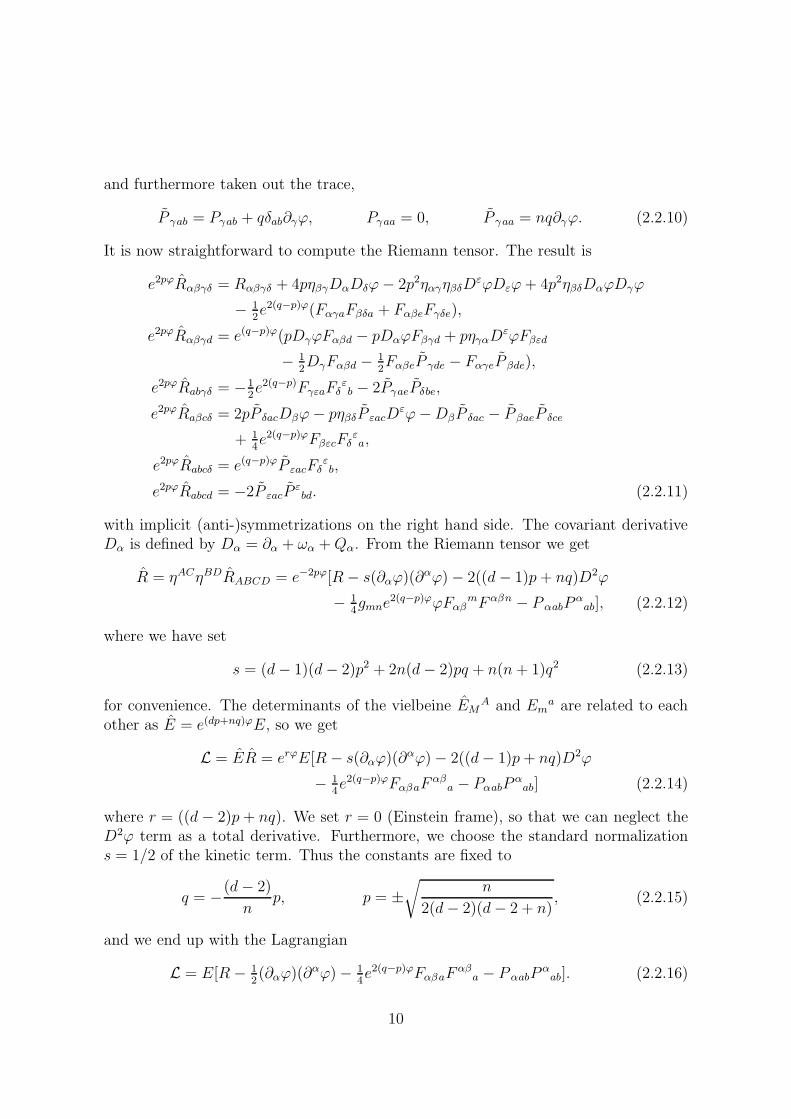
It is now straightforward to compute the Riemann tensor. The result is
for convenience. The determinants of the vielbeine EMA and Em
a are related to eachother as E = e(dp+nq)ϕE, so we get
L = ER = erϕE[R − s(∂αϕ)(∂αϕ)− 2((d− 1)p+ nq)D2ϕ
− 14e2(q−p)ϕFαβaF
αβa − PαabP
αab] (2.2.14)
where r = ((d − 2)p + nq). We set r = 0 (Einstein frame), so that we can neglect theD2ϕ term as a total derivative. Furthermore, we choose the standard normalizations = 1/2 of the kinetic term. Thus the constants are fixed to
q = −(d− 2)
np, p = ±
√
n
2(d− 2)(d− 2 + n), (2.2.15)
and we end up with the Lagrangian
L = E[R − 12(∂αϕ)(∂
αϕ)− 14e2(q−p)ϕFαβaF
αβa − P αabP
αab]. (2.2.16)
10
This Lagrangian is invariant globally under GL(n) and locally under SO(n). To un-derstand what this means, we rewrite the Lagrangian in terms of matrices. We let Vbe the internal vielbein, which is an n × n matrix with determinant one and compo-nents Vma = Em
a. Furthermore, we let M be the symmetric n × n matrix V V t withcomponents
Mmn = (V V t)mn = VmaVna = EmaEn
a. (2.2.17)
Finally, we interpret Pαab and F αβa as the components of a traceless symmetric n× nmatrix Pα and an n× 1 column matrix F αβ . After a little algebra we find that
tr (PαPα) = −tr (∂αM∂αM−1), (2.2.18)
and the last two terms in the Lagrangian (to be multiplied with the overall factor E)can be written
−tr (PαPα)− 1
4e2(q−p)ϕFαβ
tV V tF αβ = tr (∂αM∂αM−1)− FαβtMF αβ . (2.2.19)
First we show that this part of the Lagrangian has a global SL(n) symmetry. Considerthe transformations
V → LV, Fαβ → (Lt)−1Fαβ, (2.2.20)
where L is a constant n× n matrix with determinant one. This means that we replaceV by LV and F by (Lt)−1F everywhere. Then M and M−1 transform as
M → LMLt, M−1 → (L−1)tM−1L−1. (2.2.21)
Since L is constant and the trace is invariant under cyclic permutations, we get
tr (∂αM∂αM−1) → tr (∂αM∂αM−1), (2.2.22)
and it is also easy to see that
FαβtV V tF αβ → Fαβ
tV V tF αβ. (2.2.23)
The first two terms in the Lagrangian (2.2.16) and the overall factor E do not dependon V or F , so it follows that the whole expression is invariant. Consider now thetransformation
V → V J, (2.2.24)
where J is an orthogonal n× n matrix, leaving F invariant. Then we get
M = V V t → V JJ tV t = V JJ−1V t =M, (2.2.25)
11
so the Lagrangian is invariant even if J is not constant. The set of all n× n matriceswith determinant one form the Lie group SL(n) under matrix multiplication, and thesubgroup SO(n) consists of all orthogonal n×n matrices. What we have shown is thatthe Lagrangian (2.2.16) has a global SL(n) symmetry and a local SO(n) symmetry.Alternatively, this can be shown by considering infinitesimal transformations. Thenone acts with matrices that belong to the corresponding Lie algebras instead, sl(n)and its subalgebra so(n). They consist of all traceless and all antisymmetric n × nmatrices, respectively. Thus Pα itself is an element of the Lie algebra sl(n), but not ofso(n), whereas M is an element of the Lie group SL(n). The antisymmetric part Qα
of the Maurer-Cartan form, which dropped out of the Lagrangian, is an element of theLie algebra so(n) as well as of sl(n). Upon inclusion of the dilaton, or the trace partof the Maurer-Cartan form, SL(n) and sl(n) extends to GL(n) and gl(n).
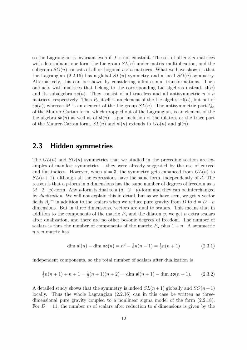
2.3 Hidden symmetries
The GL(n) and SO(n) symmetries that we studied in the preceding section are ex-amples of manifest symmetries – they were already suggested by the use of curvedand flat indices. However, when d = 3, the symmetry gets enhanced from GL(n) toSL(n + 1), although all the expressions have the same form, independently of d. Thereason is that a p-form in d dimensions has the same number of degrees of freedom as a(d−2−p)-form. Any p-form is dual to a (d−2−p)-form and they can be interchangedby dualization. We will not explain this in detail, but as we have seen, we get n vectorfields Aµ
m in addition to the scalars when we reduce pure gravity from D to d = D−ndimensions. But in three dimensions, vectors are dual to scalars. This means that inaddition to the components of the matrix Pα and the dilaton ϕ, we get n extra scalarsafter dualization, and there are no other bosonic degrees of freedom. The number ofscalars is thus the number of components of the matrix Pα plus 1 + n. A symmetricn× n matrix has
dim sl(n)− dim so(n) = n2 − 12n(n− 1) = 1
2n(n + 1) (2.3.1)
independent components, so the total number of scalars after dualization is
12n(n + 1) + n + 1 = 1
2(n+ 1)(n+ 2) = dim sl(n+ 1)− dim so(n + 1). (2.3.2)
A detailed study shows that the symmetry is indeed SL(n+1) globally and SO(n+1)locally. Thus the whole Lagrangian (2.2.16) can in this case be written as three-dimensional pure gravity coupled to a nonlinear sigma model of the form (2.2.18).For D = 11, the number m of scalars after reduction to d dimensions is given by the
12
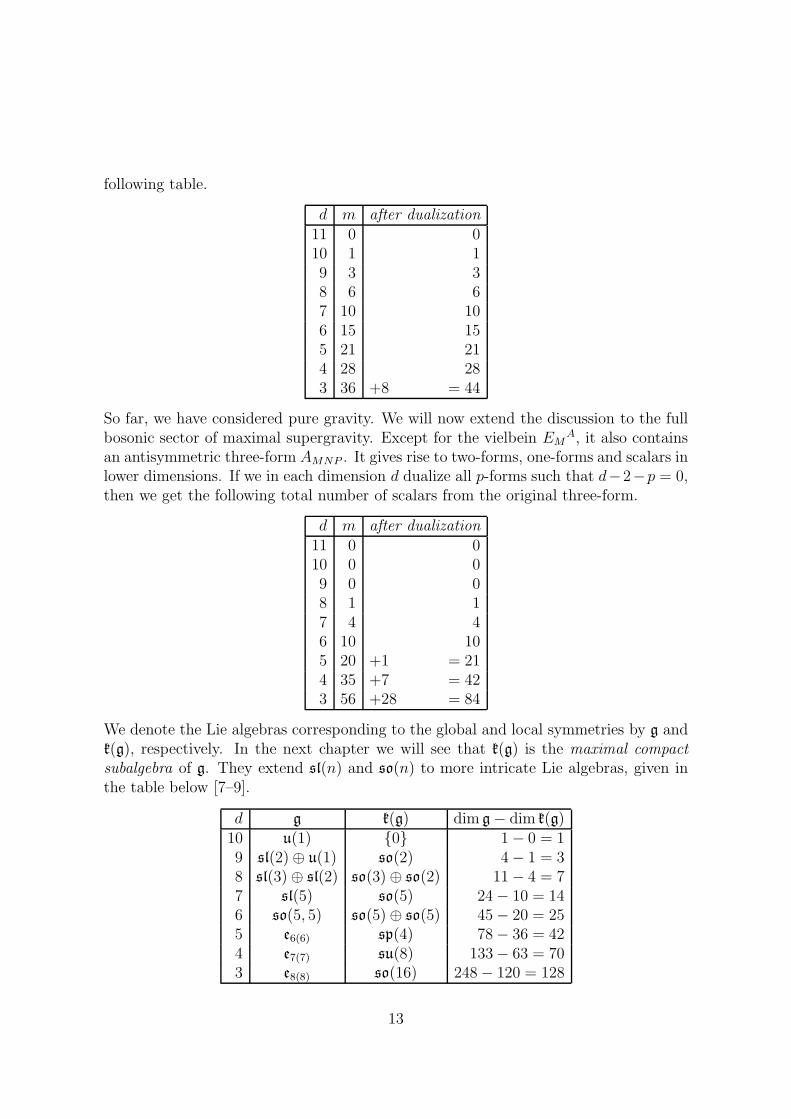
following table.
d m after dualization11 0 010 1 19 3 38 6 67 10 106 15 155 21 214 28 283 36 +8 = 44
So far, we have considered pure gravity. We will now extend the discussion to the fullbosonic sector of maximal supergravity. Except for the vielbein EM
A, it also containsan antisymmetric three-form AMNP . It gives rise to two-forms, one-forms and scalars inlower dimensions. If we in each dimension d dualize all p-forms such that d−2−p = 0,then we get the following total number of scalars from the original three-form.
d m after dualization11 0 010 0 09 0 08 1 17 4 46 10 105 20 +1 = 214 35 +7 = 423 56 +28 = 84
We denote the Lie algebras corresponding to the global and local symmetries by g andk(g), respectively. In the next chapter we will see that k(g) is the maximal compactsubalgebra of g. They extend sl(n) and so(n) to more intricate Lie algebras, given inthe table below [7–9].
As for pure gravity, we will not show this is in detail, but try to convince the readerby counting the degrees of freedom. For any 3 ≤ d ≤ 10, the dimension of the cosetp = g⊖ k(g), (which is the rightmost number in the last table) coincides with the sumof the number of scalars after dualization (which are the numbers in the two previoustables).
There is a Lie algebra en (with split real form en(n)) for any n ≥ 6, not only forn = 6, 7, 8 as in the table above. In fact, we will see that the algebras g for d = 6 andd = 7 can be considered as en for n = 5 and n = 4, respectively. It is therefore naturalto expect that also e9, e10 and e11 show up in the reduction to two, one or even zerodimensions. However, we cannot proceed in the same way after d = 3, since scalarsbecome dual to scalars in two dimensions. On the mathematical side, this difficulty isreflected by the fact that the Lie algebras en are infinite-dimensional for n ≥ 9. Wewill see how one can handle this in chapter 5, but first we need some more generalbackground about Lie algebras.
14
3Lie algebras
The simple finite-dimensional Lie algebras were classified by Cartan and Killing along time ago. In this classification, e6, e7, e8 are included as exceptional Lie algebras(together with f4 and g2). As we will see in this chapter, there is a natural way toextend the classification, such that also some infinite-dimensional Lie algebras can beincluded. In particular, Lie algebras en can be defined as such Kac-Moody algebrasfor any n ≥ 4. When we talk about exceptional Lie algebras in this thesis, we referto this generalized meaning. All Lie algebras that we consider are defined over thecomplex numbers if nothing else is stated. For introductions to Lie algebras and theirrepresentations, we recommend [39, 40].
3.1 Kac-Moody algebras
The Cartan-Killing classification of simple finite-dimensional Lie algebras is based onthe assignment of a (unique) Cartan matrix to any such Lie algebra, which describesit completely. By relaxing one of the conditions that a Cartan matrix must satisfy,one obtains a much larger class of Lie algebras, called Kac-Moody algebras [41–46].We will henceforth talk about Cartan matrices in this generalized meaning. The cor-respondence between Cartan matrices and Kac-Moody algebras is one-to-one up toisomorphisms between Kac-Moody algebras and permutations of the index set labelingrows and columns in the Cartan matrix [47].
In section 3.1.1, we will review the classification of Cartan matrices, following [48].Since there is a one-to-one correspondence between Cartan matrices and Kac-Moodyalgebras this will then correspond to a classification of Kac-Moody algebras. In section3.1.3 we will explain how a Kac-Moody algebra is constructed from its Cartan matrixA if detA 6= 0.
15
3.1.1 Cartan matrices
Let A be an indecomposable square matrix with integer entries Aij . If Aii = 2 alongthe diagonal (no summation) and Aij ≤ 0 for i 6= j, with
Aij = 0 ⇔ Aji = 0, (3.1.1)
then A is called a Cartan matrix.
For any column matrix a, we write a > 0 if all entries are positive, and a < 0 if allentries are negative. We now define an r × r Cartan matrix A to be
• finite if Ab > 0,
• affine if Ab = 0,
• indefinite if Ab < 0
for some r × 1 matrix b > 0. One and only one of these three assertions is valid forany A, and in the affine case, b is uniquely defined up to normalization [48,49]. AffineCartan matrices can also be characterized in the following way.
• A is affine if and only if detA = 0 and deletion of any row and the correspondingcolumn gives a direct sum of finite Cartan matrices.
As we will describe in section 3.1.3, any Cartan matrix defines uniquely a Liealgebra, and all Lie algebras that can be obtained in this way are called Kac-Moodyalgebras. Thus we can say that a Kac-Moody algebra is finite, affine or indefiniteif the same holds for its Cartan matrix. Finite Kac-Moody algebras are then nothingbut simple finite-dimensional Lie algebras, and their construction gives us back theCartan-Killing classification. Also the affine Kac-Moody algebras are well understood,as certain extensions of finite algebras. On the other hand, the indefinite Kac-Moodyalgebras are neither fully classified nor well understood. We need to impose furtherconditions in order to study them along with the finite and affine algebras. In whatfollows we will always require an indefinite Cartan matrix A to be symmetrizable,which means that there is a diagonal matrix D with positive diagonal entries suchthat DA is symmetric. Then D is unique up to an overall factor. All finite and affinealgebras are already symmetrizable [48, 49]. It now follows that
• A is finite if and only if A is symmetrizable and the symmetrized matrix hassignature (+ · · ·++),
• A is affine if and only if A is symmetrizable and the symmetrized matrix hassignature (+ · · ·+ 0 ).
16
Analogously, we define A to be Lorentzian if A is symmetrizable and the symmetrizedmatrix has signature (+ · · · + −). (With signature we mean the number of positive,negative or zero eigenvalues. Their order does not matter.) Clearly, the Lorentzianalgebras form a subclass of the class of indefinite algebras, but we can restrict it evenfurther. Similarly to the characterization of the affine case above, we define hyperbolicCartan matrices in the following way.
• A is hyperbolic if and only if detA < 0 and deletion of any row and the corre-sponding column gives a direct sum of affine or finite matrices.
It can be shown that any hyperbolic Cartan matrix is Lorentzian. We say that aKac-Moody algebra is Lorentzian or hyperbolic if the same holds for its Cartanmatrix.
3.1.2 Dynkin diagrams
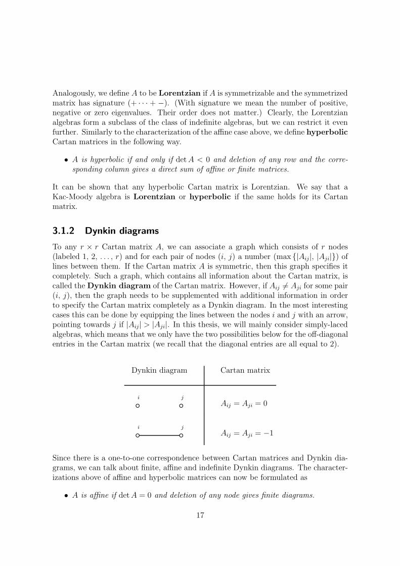
To any r × r Cartan matrix A, we can associate a graph which consists of r nodes(labeled 1, 2, . . . , r) and for each pair of nodes (i, j) a number (max |Aij|, |Aji|) oflines between them. If the Cartan matrix A is symmetric, then this graph specifies itcompletely. Such a graph, which contains all information about the Cartan matrix, iscalled the Dynkin diagram of the Cartan matrix. However, if Aij 6= Aji for some pair(i, j), then the graph needs to be supplemented with additional information in orderto specify the Cartan matrix completely as a Dynkin diagram. In the most interestingcases this can be done by equipping the lines between the nodes i and j with an arrow,pointing towards j if |Aij| > |Aji|. In this thesis, we will mainly consider simply-lacedalgebras, which means that we only have the two possibilities below for the off-diagonalentries in the Cartan matrix (we recall that the diagonal entries are all equal to 2).
Dynkin diagram Cartan matrix
i j
Aij = Aji = 0
i j
Aij = Aji = −1
Since there is a one-to-one correspondence between Cartan matrices and Dynkin dia-grams, we can talk about finite, affine and indefinite Dynkin diagrams. The character-izations above of affine and hyperbolic matrices can now be formulated as
• A is affine if detA = 0 and deletion of any node gives finite diagrams.
17
• A is hyperbolic if detA < 0 and deletion of any node gives affine or finite dia-grams.
Permutation of rows and (the corresponding) columns in A corresponds to rela-beling the nodes in the Dynkin diagram. The condition that a Cartan matrix shouldbe indecomposable corresponds to the condition that a Dynkin diagram should beconnected.
3.1.3 The Chevalley-Serre relations
We will now describe how a Lie algebra can be constructed from a given Cartan matrixA or, equivalently, from its Dynkin diagram. The Lie algebra g′ obtained in this wayis called the derived Kac-Moody algebra of A. The Kac-Moody algebra g of A isthen defined as a certain extension of g′ in the case when A is affine. We will explainthis in chapter 5.4. If A is finite or indefinite, then g coincides with g′.
In the construction of the Lie algebra g′ from its Cartan matrix A, one starts with3r generators ei, fi, hi satisfying the Chevalley relations (no summation)
[ei, fj ] = δijhj , [hi, hj ] = 0,
[hi, ej ] = Ajiej , [hi, fj ] = −Ajifj . (3.1.2)
The elements hi span the abelian Cartan subalgebra h. The derived Kac-Moodyalgebra g′ is then generated by ei and fi modulo the Serre relations (no summation)
(ad ei)1−Aji
ej = 0, (ad fi)1−Aji
fj = 0. (3.1.3)
It follows from the Chevalley relations (3.1.2) that g, except for the Cartan elements,is spanned by the set of multiple commutators
for all n ≥ 1, which is restricted by the Serre relations (3.1.3). It also follows from(3.1.2) that these multiple commutators are eigenvectors of ad h for any h ∈ h, andthus each of them defines an element µ in the dual space of h, such that µ(h) is thecorresponding eigenvalue. These elements µ are the roots of g and the eigenvectors arecalled root vectors. In particular, ei are root vectors of the simple roots αi, whichform a basis of the dual space of h. In this basis, an arbitrary root µ = µiαi has integercomponents µi, either all non-negative (if µ is a positive root) or all non-positive (ifµ is a negative root).
For finite Kac-Moody algebras, the space of root vectors corresponding to any rootis one-dimensional. Furthermore, if µ is a root, then −µ is a root as well, but no othermultiples of µ. For any positive root µ of a finite Kac-Moody algebra g, we let eµ be a
18
root vector corresponding to µ like the first one in (3.1.4), with αi1+αi1+ · · ·+αin = µ.In what follows we will write such a multiple commutator as
[ei1 , ei2 , . . . , ein ], (3.1.5)
assuming the same ordering as in (3.1.4). Then eµ is fixed up to a sign, and we let fµbe the root vector
[−fi1 , −fi2 , . . . , −fin ], (3.1.6)
corresponding to −µ. Thus a basis of g is formed by these root vectors eµ, fµ for allpositive roots µ, and by the Cartan elements hi for all i = 1, 2, . . . , r.
The reason for the minus signs in (3.1.6) is that we can now also associate anelement hµ in the Cartan subalgebra to each positive root in a way such that therelations (3.1.2) for i = j extend from the simple roots to all positive roots,
Now we can also define an involution ω on the finite Kac-Moody algebra g by
ω(hµ) = −hµ, ω(eµ) = −fµ, ω(fµ) = −eµ, (3.1.8)
for all positive rots µ = µiαi, where hµ = µihi. This involution is called the Chevalley
involution.For an arbitrary derived Kac-Moody algebra, there can bem ≥ 1 linearly dependent
root vectors to a given root, which is then said to have multiplicity m. Then the rootvectors eµ and fµ are not uniquely given by the root µ up to a sign, as for finite algebras.In order to distinguish between linearly independent root vectors corresponding to thesame root, we must also specify the order of the simple root vectors in the multiplecommutators. The Chevalley involution is in this general case defined by
ω(hi) = −hi, ω(ei) = −fi, ω(fi) = −ei (3.1.9)
for the Chevalley generators, and then extended to the whole algebra by the homo-morphism property.
3.1.4 The Killing form
In any finite-dimensional Lie algebra g we can define a bilinear form κ, called theKilling form, by κ(x, y) = tr (ad x ad y). The Killing form is symmetric and invari-ant under the adjoint action of the algebra,
κ([a, b], c) + κ(b, [a, c]) = 0. (3.1.10)
19
Furthermore it is non-degenerate if and only if the Lie algebra is semisimple. If g
is simple and finite-dimensional then κ can equivalently, up to an overall factor, bedefined by
κ(ei, fj) = Dij , κ(hi, hj) = (DA)ij, (3.1.11)
for all i, j = 1, 2, . . . , r, where D is a diagonal matrix (unique up to an overall factor)such that DA is symmetric. In all other cases the Killing form is defined to be zero. Itcan then be extended to the full algebra by the symmetry and invariance properties,together with the Chevalley relations. The Killing form will then be symmetric andinvariant by construction, but also non-degenerate. Moreover, these properties definethe Killing form uniquely up to automorphisms and an overall normalization.
3.1.5 The maximal compact subalgebra
The maximal compact subalgebra k(g) of a Kac-Moody algebra g is defined as thesubalgebra of g which is pointwise fixed by the Chevalley involution. Thus it consistsof all elements x + ω(x), where x ∈ g. A basis is given by eµ − fµ for all root vectorseµ, fµ. Similarly, we define the coset p(g) to be the subspace consisting of all elementsx−ω(x). Thus it is spanned by all elements eµ+ fµ, and the Cartan generators. Withrespect to the Killing form, the maximal compact subalgebra k(g) is negative-definite,the coset p(g) is positive-definite away from the Cartan subalgebra, and these twosubspaces of g are orthogonal complements to each other. Moreover, we have
[k, k] ⊂ k, [k, p] ⊂ p, [p, p] ⊂ k, (3.1.12)
so the subspace p(g) constitutes a representation of the subalgebra k(g), but p(g) doesnot close under the Lie bracket. The decomposition g = k + p is called the Cartan
decomposition.The maximal compact subalgebra k(g) of a Kac-Moody algebra g is itself a Kac-
Moody algebra or a direct sum of Kac-Moody algebras as long as g is finite. As wewill see, this is in general not true if g is infinite-dimensional.
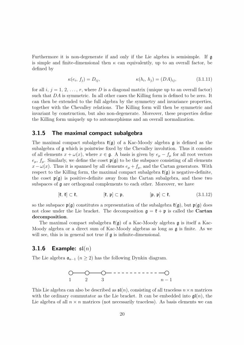
3.1.6 Example: sl(n)
The Lie algebra an−1 (n ≥ 2) has the following Dynkin diagram.
1 2 3 n− 1
This Lie algebra can also be described as sl(n), consisting of all traceless n×n matriceswith the ordinary commutator as the Lie bracket. It can be embedded into gl(n), theLie algebra of all n× n matrices (not necessarily traceless). As basis elements we can
20
take all matrices Kab for a, b = 1, 2, . . . , n, where the entry in row a and column b is
one, and all other entries are zero. The commutation relations are then
[Kab, K
cd] = δcbK
ad − δadK
cb. (3.1.13)
The subalgebra sl(n) is obtained by factoring out the one-dimensional ideal spannedby the identity matrix. Then we can write the Chevalley generators as
ha = Ka+1a+1 −Ka
a, ea = Ka+1a, fa = Ka
a+1. (3.1.14)
and we see that the Chevalley involution is given by minus the transpose. Thus themaximal compact subalgebra of sl(n) is so(n), consisting of all antisymmetric matrices.By embedding sl(n) into gl(n), the Killing form can be written
κ(Kab, K
cd) = δcbδ
ad +mδabδ
cd (3.1.15)
for an arbitrary number m (the terms involving m cancel out for the sl(n) subalgebra).For two arbitrary traceless matrices x and y, this gives κ(x, y) = tr (xy).
3.2 Graded Lie algebras
Kac-Moody algebras are special cases of graded Lie algebras. In fact, it was the interestin graded Lie algebras that led Kac (independently of Moody) to the study of Kac-Moody algebras [48].
With a graded (or Z-graded) Lie algebra we mean a Lie algebra that can be writtenas a direct sum of subspaces gk ⊂ g for all integers k, such that
[gm, gn] ⊆ gm+n (3.2.1)
for all integers m, n. If there is a positive integer m such that g±m 6= 0 but g±k = 0for all k > m, then the Lie algebra g is (2m+ 1)-graded. We will occasionally use thenotation g± = g±1 + g±2 + · · · . A graded involution τ on the Lie algebra g is anautomorphism such that τ 2(x) = x for any x ∈ g and τ(gk) = g−k for any integer k. Acharacteristic element [50, 51] in a graded Lie algebra g is an element d such that
[d, x] = kx (3.2.2)
if x ∈ gk, for all integers k. Any semisimple finite-dimensional graded Lie algebra hasa characteristic element [52].
3.2.1 Graded Kac-Moody algebras
Consider a simple Kac-Moody algebra g and choose a simple root αi. For any negative(positive) integer k, let gk be the subspace of g spanned by all root vectors eµ (fµ) such
21
that the component µi of the root µ, corresponding to αi in the basis of simple roots,is equal to |k|. Let g0 be spanned by all Cartan generators hj and all root vectors eµand fµ such that µi = 0. In this way any simple root αi gives a grading of g.
Generally, any set of simple roots αi1 , αi2 , . . . , αin gives a grading of g where gkis spanned by all root vectors eµ or fµ such that µi1 + µi2 + · · · + µin = ±k and, ifk = 0, the Cartan generators. Any grading of a simple finite-dimensional Lie algebrag, such that [gi, gj ] = gi+j for all integers i, j, is given by a set of simple roots in thisway [52]. With a graded Kac-Moody algebra we will always mean a simple Kac-Moodyalgebra togehter with such a grading for some set S of simple roots. It follows thatthe Chevalley involution is a graded involution in a graded Kac-Moody algebra. Anygraded involution τ together with the Killing form κ on g induces a non-degeneratebilinear form on the subspace g−1, given by
(x, y) = κ(x, τ(y)) (3.2.3)
for all x, y ∈ g−1. We call this the bilinear form associated to τ . A finite or indefinitegraded Kac-Moody algebra has a unique characteristic element d in the Cartan subal-gebra. Its components in the basis of Cartan generators are given by the solution to theequation Ad = b where A is the Cartan matrix of g and bi = 1 if αi belongs to the setS that defines the grading, and bi = 0 otherwise. Since g is simple, detA 6= 0 and theequation has a unique solution. The subalgebra g0 is a direct sum of one-dimensionalLie algebras spanned by the Cartan elements corresponding to the set S and a directsum g0
′ of derived Kac-Moody algebras. Their Dynkin diagrams are obtained fromthat of g by deleting the nodes that correspond to the set S of simple roots.
3.2.2 Level decomposition
The grading of a Kac-Moody algebra comes with a level decomposition of its adjointrepresentation under the g0
′ subalgebra. Since [g0, gm] ⊂ gm as a special case of (3.2.1),the subspace gm ⊂ g constitutes a representation rm of g0
′, which is the representationat level m in the level decomposition. It follows that rm is a subrepresentation of them-fold tensor product (r1)
m, irreducible or not. At level 2, only the antisymmetricpart of r1 ⊗ r1 occurs, because of antisymmetry of the Lie bracket. At level 3, thetotally antisymmetric part of r1 ⊗ r1 ⊗ r1 is ruled out because of the Jacobi identity.In addition, the Serre relations restrict the representation at any nonzero level.
3.2.3 The universal graded Lie algebra
In this section we will show how any vector space V naturally gives rise to a gradedLie algebra
U(V ) = U− + U0 + U+. (3.2.4)
22
As we will see, any graded Lie algebra g such that [g−m, g−n] = g−m−n for all positiveintegersm, n can be embedded in U(g−1) [53]. This will be important when we considergeneralized Jordan triple systems in the next chapter. Moreover, any graded Lie algebracan be embedded into U(g−), which gives a nonlinear realization of g [52]. A well knownexample of this is the conformal realization of so(2, d), as we explain in Paper III.
With an operator of order p ≥ 1 on a vector space V we mean a p-linear mapV p → V . Let A and B be operators on a vector space V of order p and q, respectively.Then we define the composition A B to be an operator on V of order p+ q − 1 by
(A B)(v1, . . . , vp+q−1)
=
p∑
m=1
∑
A(vn1, . . . , vnm−1
, B(vnm, . . . , vnm+q−1
), vq+m, . . . , vp+q−1) (3.2.5)
where the second sum goes over all distinct values of the q indices nm, . . . , nm+q−1
chosen among the m + q − 1 values 1, . . . , m + q − 1, such that nm < · · · < nm+q−1
and the remaining indices are ordered such that n1 < · · · < nm−1. For any integerk ≥ 0, let Uk be the vector space spanned by all operators on V of order k+1, and letU0 + U+ be the direct sum of all these vector spaces [53]. Then U0 + U+ is a gradedLie algebra under the commutator
[A, B] = A B − B A. (3.2.6)
A basis element A in Up−1 for p ≥ 1 is thus an operator on V of order p, but it canalso be viewed as a linear map V → U p−2 by
The vector spaces Uk for k ≥ −1 can be defined recursively in this way, starting fromU−1 = V . We will in the continuation use this definition of Uk instead of the one aboveby Kantor [53]. One reason for this is that (3.2.5) and (3.2.6) then can be replaced bythe simple formula
[A, B] = (ad A) B − (ad B) A, (3.2.8)
where, if B is of order zero, [A, B(v)] should be read as A(B(v)) for any v in V . Itis straightforward to show by induction that the two definitions of the Lie bracket areequivalent.
Having defined U+ and U0, we complete the vector space U(V ) by defining U− asthe free Lie algebra generated by V = U−1, where U−k, for any k ≥ 1, is spanned byall multiple commutators [v1, v2, . . . , vk]. We extend the Lie algebra structure on thesubspaces U− and U0 + U+ to the whole of U(V ) by
[A, v] = A(v) (3.2.9)
23
for any A in U 0 + U+ and any v in V . Since U−(V ) is generated by elements in V ,this defines all commutation relations between U− and U0+ U+ by the Jacobi identity.The resulting algebra U(V ) is the universal graded Lie algebra of V [53].
Any graded Lie algebra g such that [g−m, g−n] = g−m−n for all positive integersm, n is isomorphic to the direct sum
(U−/D)⊕ U0 ⊕ U+ ⊂ U(g−1), (3.2.10)
where U0 ⊕U+ is a certain subalgebra of U0 ⊕ U+, and D is a graded ideal of U− [53].(This means that D is the direct sum of its subspaces D ∩ Uk for all k.)
In fact, it is possible to embed any graded Lie algebra g in a universal graded Liealgebra U(V ), such that g is entirely contained in U−1 + U 0 + U+. But then we mustlet the vector space g be the whole of g−, and not only g−1. Furthermore, the basiselements in g are mapped onto symmetric operators in U 0 + U+. An operator A on Vof order p is symmetric if
for all 1 ≤ i, j ≤ p. Then there is a corresponding map a : V → V defined by
a(v) = A(v, . . . , v). (3.2.12)
Conversely, A is uniquely given by a, so we can identify A with a as an element inU−1 + U 0 + U+. The composition of a with another such element b is a symmetricoperator as well, given by
(a b)(v) = pA(b(v), v, . . . , v). (3.2.13)
Let M(V ) be the subalgebra of U−1 + U 0 + U+ spanned by all symmetric operators.Then M(V ) is a graded Lie algebra with M−k = 0 for k ≥ −2.
It has been shown [52] (see also [54]) that there is an injective homomorphismχ : g →M(g−) given by
χ(u) : x 7→
(
ad x
1− e−ad xPe−ad x
)
(u), (3.2.14)
where P is the projection onto U− along U0 + U+, and the ratio should be consideredas the power series
ad x
1− e−ad x= 1 +
ad x
2+
(ad x)2
12−
(ad x)4
720+ · · · . (3.2.15)
Since g is graded, χ induces a grading on χ(g). However, this is not the same gradingas the one that χ(g) is equipped with as a subalgebra of U−1 + U 0 + U+.
24
The grading that χ induces on χ(g) can be defined onM(V ) for an arbitrary vectorspace V , that is a direct sum of (infinitely many) subspaces V1, V2, . . .. Let A be anelement in M(V ) (that not necessarily belongs to one of the subspaces Mk). Then wecan write A(v) as a sum of An(v) for all n = 1, 2, . . ., where An is a map V → Vn.Suppose that An is a (p1 + p2 + · · · )-linear map
An : (V1)p1 × (V2)
p2 × · · · → Vn, (3.2.16)
symmetric under permutation of elements that belong to the same vector space Vm.(In general, An will be a sum of such maps.) Then we say that A has grade p ifp1 + 2p2 + 3p3 + · · · = n + p for all n. Note that the grade can also be negative.
As before, we can identify A as a symmetric operator of grade p with a correspondingmap a : V → V . Then the composition a b of a and another symmetric operator b,of grade q, is now the symmetric operator of grade p+ q given by
for all n = 1, 2, . . ., and a Lie bracket as usual by [a, b] = a b− b a. It follows thatM(V ) is a graded Lie algebra also with this grading, which is preserved by the inverseof the homomorphism χ for V = g−1.
25
26
4Generalized Jordan triple systems
In the end of the preceding chapter, we saw that any vector space V gives rise to agraded Lie algebra U(V ). Furthermore, we said that any graded Lie algebra g generatedby its g±1 subspaces can be embedded in U(V ) for some vector space V . In this chapterwe will see how a given graded Lie algebra can be extracted from U(V ). This is done byidentifying V with g−1 and adding extra structure to this vector space, correspondingto the properties of g. The result is a generalized Jordan triple system.
In this chapter we will study various kinds of generalized Jordan triple systems andtheir associated graded Lie algebras. One reason for this is that we might learn moreabout the exceptional Lie algebras appearing in supergravity by studying their corre-sponding generalized Jordan triple systems. We can also go in the opposite directionand learn more about a generalized Jordan triple system by studying its associatedgraded Lie algebra. In the end of this chapter we will explain how a certain kind ofgeneralized Jordan triple systems, called three-algebras, are used in three-dimensionalsuperconformal theories to describe multiple M2-branes. In Paper IV we show howthe theory can equivalently be formulated in terms of the associated graded Lie alge-bra. Such a formulation might lead to a generalization of the theory, since g−1 (thethree-algebra) is only one of many subspaces of a graded Lie algebra g.
4.1 Preliminaries
A triple system is a vector space V together with a trilinear map
V × V × V → V, (x, y, z) 7→ (xyz), (4.1.1)
called triple product. Let g be a graded Lie algebra with a graded involution τ .Then g−1 is a triple system with the triple product
(xyz) = [[x, τ(y)], z]. (4.1.2)
27
As a consequence of the Jacobi identity and the fact that τ is an involution, this tripleproduct satisfies the identity
Any triple system that satisfies (4.1.3) is called a generalized Jordan triple system.Let V be an arbitrary generalized Jordan triple system (not necessarily derived from
a Lie algebra as above) of dimensionm, and let TA be a basis of V , forA = 1, 2, . . . , m.In analogy with Lie algebras we introduce structure constants fABC
D for V , whichspecify the triple product by
(TAT BT C) = fABCDT
D. (4.1.4)
The identity (4.1.3) can then be written
fABCDf
EFDG − fEFC
DfABD
G = fEFADf
DBCG − fFEB
DfADC
G. (4.1.5)
4.2 Normed triple systems
Suppose now that g has a non-degenerate bilinear form κ, which is symmetric andinvariant,
and such that κ(gm, gn) = 0 whenever m + n 6= 0. The obvious example of such abilinear form is the Killing form in a graded Kac-Moody algebra, but we want to bemore general here and allow for Lie algebras that are not of Kac-Moody type. Togetherwith the involution τ , the bilinear form κ on g induces a bilinear form on g−1 by
h(x, y) = κ(x, τ(y)). (4.2.2)
We call h the bilinear form associated to τ . Suppose that h is symmetric (whichmeans that κ is preserved by τ). Then we call g a nicely graded Lie algebra. As aconsequence of the invariance (4.2.1), we have
If this identity holds for some symmetric bilinear form h defined on a generalized Jordantriple system V , then we say that h is a metric on V , and that V is a normed triplesystem. Thus any nicely graded Lie algebra gives rise to a normed triple system. Weintroduce the components hAB of the metric by
hAB = h(TA, T B). (4.2.4)
We use hAB and the inverse hAB to raise and lower indices, for example,
TA = hABTB, fABCD = fABC
EhDE . (4.2.5)
The identity (4.2.3) can now be written
fABCD = fCDAB = fBADC = fDCBA. (4.2.6)
28
4.3 The associated Lie algebra
In section 3.2.3, we defined the universal graded Lie algebra U(V ) of an arbitrary vectorspace V . We will now assume that V is a generalized Jordan triple system, and usethis to define a subalgebra of U(V ).
For any pair of basis elements (TA, T B) of V , we define the linear map
SAB : V → V, SAB(T C) = fABCDT
D. (4.3.1)
Thus (4.1.3) can be written
[SAB, SCD] = fABCES
ED − fBADES
CE . (4.3.2)
For any basis element TA, we also define the linear map
TA : V → End V, TA(T B) = SAB, (4.3.3)
Let L0 be the subspace of U0 spanned by all SAB, and let L+ be the subspace of U+
generated by all elements TA in U1. Furthermore, let L− be a Lie algebra isomorphic toL+, with the isomorphism denoted by τ . Thus L− is generated by all elements τ(TA).Consider the vector space
L(V ) = L− ⊕ L0 ⊕ L+. (4.3.4)
We can extend the Lie algebra structures on each of these subspaces to a Lie algebrastructure on the whole of L(V ), by the relations
[SAB, T C] = fABCDT
D,
[TA, τ(T B)] = SAB,
[SAB, τ(T C)] = −fBACDτ(T
D). (4.3.5)
The commutator between two arbitrary elements in two different subspaces L+, L− orL0 can be derived from (4.3.5) by the Jacobi identity since L+ and L− are generatedby TA and τ(TA), respectively. We can also extend the isomorphism τ between thesubalgebras L− and L+ to a graded involution on the Lie algebra L(V ). On L−, itis given by the inverse of the original isomorphism, τ(τ(TA)) = TA, and on L0 byτ(SAB) = −SBA.
We call L(V ) the associated Lie algebra to the generalized triple system V . (Thisdefinition differs from the definition by Kantor of the Lie algebra L(V ) in [52] in thatthe basis element τ(TA) of g−1 is not the same as the basis element TA of V . However,if the generalized Jordan triple system V does not contain any element a such that(axy) = 0 for all x, y in V , then we can identify TA with τ(TA) and the definitions areequivalent.)
29
If V is derived from a simple graded Lie algebra g with a graded involution τ by(4.1.2), then L(V ) is isomorphic to g. Conversely, the generalized Jordan triple systemderived from L(V ) by (4.1.2) is isomorphic to V if V is simple in the sense that thereare no nontrivial subspace W ⊂ V such that (V VW ) ⊆ W and (WV V ) ⊆ W . Thiswas shown by Kantor in [52] and we also include a proof of the first assertion in theappendix of Paper III (where we use a somewhat different notation). Thus there is aone-to-one correspondence between simple graded Lie algebras and simple generalizedJordan triple systems. In the rest of this section we will refine this to a one-to-onecorrespondence between simple nicely graded Lie algebras and simple normed triplesystems.
The basis elements of L2 are all commutators [TA, TB] in the universal graded Liealgebra U(V ) of V . Since they are elements in L2, they are linear operators V → L1.This means that [TA, T B](T C) is an element in L1 for any T C and thus is a linearmap V → EndV . We write [TA, T B] = TAB. It follows from the recursively definedcommutation relations for U(V ), that the linear map
TAB(T C) : V → EndV (4.3.6)
is given by
TAB(T C) = [TA, T B](T C) = (ad TA T B − ad T B TA)(T C)
= (ad TA)(T B(T C))− (ad TB)(TA(T C))
= [TA, SBC]− [T B, SAC]
= −fBCADT
D + fACBDT
D (4.3.7)
where we in the last step have used the commutation relations
[SAB, T C] = fABCDT
D. (4.3.8)
We can write this as
TAB(T C) = gABCDT
D, (4.3.9)
where gABCD = fACB
D − fBCAD. We note that the tensor gABC
D is antisymmetric inthe indices A and B due to the antisymmetry of the bracket [TA, T B]. In Paper III
we write (following [55]) the operator TAB as 〈TA, T B〉, or generally
〈u, v〉(x) = (uxv)− (vxu). (4.3.10)
If any triple product (uxv) is symmetric in u and v then all operators 〈u, v〉 are zero,and the associated Lie algebra L(V ) is three-graded,
L(V ) = L−1 + L0 + L1. (4.3.11)
30
In this special case, V is a Jordan triple system [56]. Conversely, if a Lie algebrag is three-graded, then the triple product (4.1.2) will automatically be symmetric in xand z and thus g−1 is a Jordan triple system.
We return to the general case, where L2 6= 0. In the same way as above we candefine a basis of L3 consisting of elements
TABC = [TAB, T C] = [[TA, TB], T C] (4.3.12)
in the universal graded Lie algebra U(V ) of V , and write
TABC(TD)(T E) = gABCDEF T
F (4.3.13)
for some tensor gABCDEF , which specifies the linear map TABC : V → U2 completely.
Again from the antisymmetry of the Lie bracket, we know that gABCDEF must be an-
tisymmetric in the first two indices. Furthermore, the Jacobi identity tells us thatgABCDE
F vanishes upon antisymmetrization in the first three upper indices. A calcula-tion like (4.3.7) for gABC
D gives
gABCDEF = 2(−fCD[A
Gg|G|B]E
F + f [A|D|B]Gg
GCEF )
= 2(−fCD[AGf
|GE|B]F + f [A|D|B]
GfGEC
F
+ fCD[AGf
B]EGF − f [A|D|B]
GfCEG
F ), (4.3.14)
which indeed satisfies g[ABC]DEF = 0. Continuing in this way, one obtains a recursion
formula for the constants gA1···AkB1···Bk−1Bk
that appear at each level k. It reads
gA1···AkB1···Bk−1Bk
= gCA3···AkB2···Bk−1BkfA1B1A2
C −∑
gCijB2···Bk−1BkfAjB1Ai
C, (4.3.15)
where the sum goes over all i, j such that 1 ≤ i < j ≤ k and Cij denotes the sequenceof indices obtained from A1 · · ·Ak by omitting Aj and replacing Ai by C, that is,
due to the antisymmetry of the Lie bracket and the Jacobi identity, but (for k ≥ 4)the tensor gA1···AkB1···Bk−1
Bkwill in addition satisfy further (anti-)symmetries. Thus we
will in this way for each k obtain a subrepresentation of the tensor product of k vectorrepresentations of sl(m), where m = dimV . The tensor g will be a linear combinationof the projectors of the representations that occur at each level. For example, if g atlevel k is symmetric under permutation of two of the k first upper indices, say A andB, then
T ···A···B··· = T ···B···A··· (4.3.18)
31
at level k. We must count these two expressions as one single element at level k sincethey define the same linear map V → Uk−1. On the other hand, they would representtwo different elements in the free Lie algebra generated by TA. Thus L+ is the algebrathat we obtain from the free Lie algebra by factoring out the ideal that is recursivelydefined by g at each level.
Suppose now that V is a normed triple system with a metric h. Since h is non-degenerate, this implies in particular that there is no element a in V such that (axy) = 0for all x, y in V , so we can identify TA with τ(TA). Thus we can write the elementsin L+ at level k as TA1···Ak and those at level −k as TA1···Ak . The graded involution issimply given by
for any k ≥ 2 (where we have raised the last index with the metric h) and κ(Lm, Ln) = 0if m+n 6= 0. Then it follows by the construction of κ and the commutation relations inL(V ) that κ is a symmetric, invariant and non-degenerate bilinear form on L(V ), andthat it is preserved by the graded involution. We have thus shown that any normedtriple system gives rise to a nicely graded Lie algebra. Conversely, as we have alreadyseen, any nicely graded Lie algebra gives rise to a normed triple system.
4.4 Extensions of generalized Jordan triple systems
In Paper III we define for any normed triple system V an infinite sequence of normedtriple systems V (n), labeled by a positive integer n, such that
dimV (n) = n dimV. (4.4.1)
Thus we can denote the basis elements of V (n) by TAa, where a = 1, 2, . . . , n. In the
special case n = 1, we can suppress the index a and identify V (n) = V (1) with V . Weintroduce a metric h(n) on V (n) by
hAaBb = h(n)(TA
a, TBb) = hABδab. (4.4.2)
The structure constants of V (n) can be expressed in those of V and the metric as
One can easily check that V (n) is a normed generalized Jordan triple system as wellas V . In Paper III we show that if the Lie algebra associated to V is a finite Kac-Moody algebra h, where the grading is given by a simple root α, then the Lie algebra g
32
associated to V (n) is a Kac-Moody algebra as well. (The subalgebra h of g should notbe confused with the Cartan subalgebra, which we called h in chapter 3.) Moreover,the Dynkin diagram of g is obtained from that of h by adding n− 1 nodes. Each nodethat we add is connected to the previous one with a single line, starting from the nodein the Dynkin diagram of h corresponding to the simple root α. The theorem can easilybe generalized to affine and hyperbolic algebras. In section 5.5.1, we will apply thismethod to show how e10 can be constructed from e8.
4.5 Three-algebras and M2-branes
As we mentioned in section 4.3, the triple product in a Jordan triple system is symmet-ric under a permutation of the first and the third element. We will not consider suchtriple systems here, but instead investigate the possibility of a triple product which isantisymmetric under a permutation of the the first and the third element,
(xyz) = −(zyx). (4.5.1)
If a generalized Jordan triple system satisfies this identity, then we call it an anti-
symmetric triple system. Thus, in addition to the identity (4.1.3), the structureconstants of a normed antisymmetric triple system satisfy
fABCD = −fCBAD = −fADCB = fCDAB (4.5.2)
and the identity (4.1.3) can be written
fED[A
CfB]
GDH = fA
DB[Gf
EH]
DC. (4.5.3)
Any associative algebra V with an anti-involution C is an antisymmetric triplesystem under the triple product
(xyz) = 12(xC(y)z − zC(y)x). (4.5.4)
For example, we can let C(x) be the transpose, inverse or hermitian conjugate of anyelement x in a matrix algebra V , that closes under C. Then it is straightforward tocheck that the identity (4.5.3) is satisfied. An important example is obtained if we takeV to be the divison algebra H of quaternions and C the conjugation, which changes signon the ‘imaginary units’ i, j, k (but leaves the real numbers unchanged). According tothe famous formula
i2 = j2 = k2 = ijk = −1 (4.5.5)
we have
(ijk) = −(jik) = 1,
(jk1) = −(kj1) = −i,
(k1i) = −(1ki) = j,
(1ij) = −(i1j) = −k (4.5.6)
33
with the triple product (4.5.4). This triple product is not only antisymmetric in x andz, but also in x and y (or y and z), so it is in fact totally antisymmetric. Moreover,since H is a normed divison algebra there is a positive-definite norm h, given by
h(x, y) = 12(xC(y) + yC(x)), (4.5.7)
and it satisfies
h(w, (xyz)) = −h(x, (wyz)). (4.5.8)
This means that if we introduce a basis TA and structure constants fABCD as before,where the last index is raised with the metric hAB = h(TA, T B), then fABCD is anti-symmetric in all four indices. If we take TA to be i, j, k, 1 for A = 1, 2, 3, 4, then wefind that
fABCD = εABCD hAB = δAB. (4.5.9)
Normed triple systems with totally antisymmetric triple products were recently usedby Bagger and Lambert in the construction of a three-dimensional theory, which wasproposed to describe multiple M2-branes [57–59]. They showed that if the scalar fieldstake values in such a triple system, called three-algebra, then one can add a non-propagating gauge field such that the resulting theory is maximally supersymmetric.The closure of the supersymmetry algebra was first shown by Gustavsson [60], usinga different but equivalent algebraic structure. In this approach, the scalar fields andthe gauge field take values in two different subspaces, called A and B, respectively,of an algebra A ⊕ B. The subspace B closes under the product and is a Lie algebra,unlike the full algebra A⊕B. If we consider the three-algebra as a generalized Jordantriple system, then we can in fact identify A and B with the subspaces L−1 and L0,respectively, of the associated Lie algebra. Their direct sum L−1⊕L0 closes and formsan algebra under a modified Lie bracket, obtained by replacing [x, y] by [x, τ(y)] forall elements x, y in L−1.
It was later proven [61–63] that the quaternionic triple system (4.5.9) is the onlynon-trivial three-algebra with positive definite metric, up to direct sums of such three-algebras. On the other hand, a generalized notion of three-algebras has gained interestsince Aharony, Bergman, Jafferis and Maldacena (ABJM) [64] constructed a supercon-formal Chern-Simons theory with less supersymmetry, N = 6 instead of the maximalnumber N = 8 in three dimensions. Bagger and Lambert showed [65] that this the-ory can be formulated in terms of a new kind of three-algebras, as a generalizationof their original model. Such a triple system is what we call a normed antisymmetrictriple system in this chapter. That is, a triple system whose structure constants satisfy(4.5.2) and (4.5.3) but are not totally antisymmetric. As we have seen, there are manyexamples of such triple systems. In this chapter we have shown that there is a one-to-one-correspondence between normed triple systems and nicely graded Lie algebras. Weuse this correspondence in Paper IV to express the ABJM theory (or the three-algebrareformulation by Bagger and Lambert) entirely in terms of the associated graded Liealgebra.
34
5The hidden symmetry algebras en
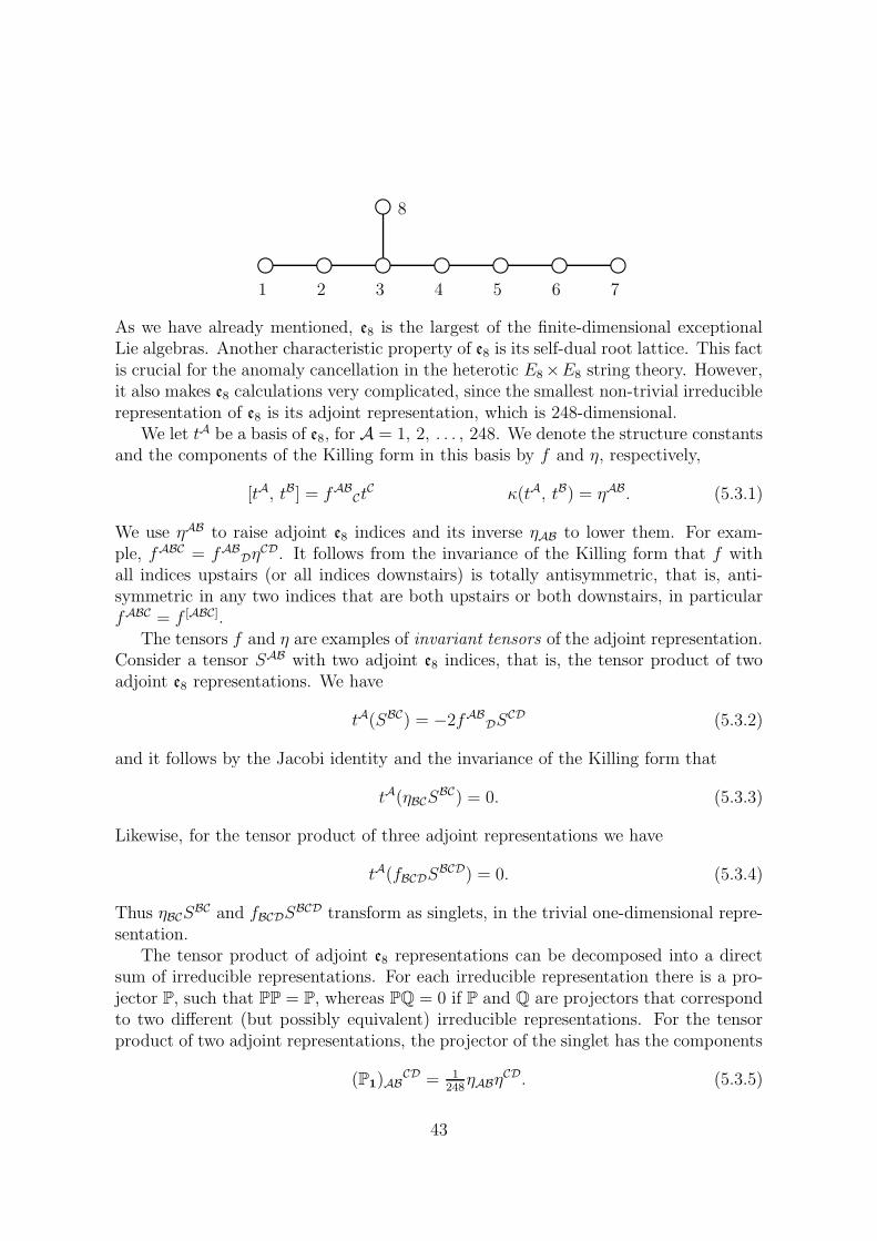
Beside the algebras an (n ≥ 1) and dn (n ≥ 4), there are three exceptional Lie algebrasthat are also simple, finite-dimensional and simply laced. These are called e6, e7 and e8.Although they do not belong to any infinite class of simple finite-dimensional algebras,they can be viewed as the first three members in an infinite family of Kac-Moodyalgebras en (n ≥ 6) with the following Dynkin diagrams.
1 2 3 4 5 n− 1
n
These algebras are infinite-dimensional for n ≥ 9. More precisely, e9 is affine, e10 ishyperbolic and e11 is Lorentzian (but not hyperbolic). In particular e8, e9 and e10 areinteresting from both a mathematical and a physical point of view, and will be devotedone section each of this chapter. First we will study the general properties of the enalgebras. These properties are in fact shared by a4 and d5, if we consider them as e4and e5, respectively. Therefore, when we talk about en in this chapter, we can assumeany n ≥ 4, if nothing else is stated. The case n = 9 will sometimes be excluded,because e9 is affine. As we saw already in chapter 2, the Lie algebras en for 4 ≤ n ≤ 8arise as hidden symmetries in the toroidal reduction of maximal supergravity from 11to d = 11− n dimensions. As we will see in the next chapter, there is also evidence fore10 as a symmetry of the unreduced theory.
5.1 Decomposition under an−1
Since the algebras en are infinite-dimensional for n ≥ 9 it is useful to study them asgraded algebras where each subspace in the grading is finite-dimensional. We choose
35
the grading given by the node labeled n in the Dynkin diagram, which is also sometimescalled the exceptional node. This node constitute the difference between sl(n) and en.Thus, according to chapter 2, it represents the difference between pure gravity and thebosonic sector of maximal supergravity. The level decomposition with respect to theexceptional node is crucial for the appearance of e10 in eleven-dimensional supergravityas we will see in chapter 6.
Following section 3.2.2 we consider the level decomposition of the adjoint repre-sentation under the subalgebra g0
′ = sl(n) corresponding to the horizontal line in theDynkin diagram. The subspace g−1 is spanned by all root vectors eµ such that thecomponent of the root µ corresponding to the simple root αn (the exceptional root)is equal to one. According to the Chevalley-Serre relations, a basis of g−1 is then theset of all multiple commutators
for all integers i, j, k such that 0 ≤ k ≤ j ≤ i ≤ n − 3 (If i = 0, this means that thesequence e3, e4, . . . , ei+2 should not appear at all, and likewise for j and k. For betterreadability, we have in (5.1.1) only written out the brackets between these sequences.)Thus we have
dim g−1 =16(n− 2)(n− 1)n (5.1.2)
and since g−1 must be an irreducible representation of g0, the only possibility is thetotally antisymmetric tensor product of either three vectors or three conjugate vectors.We write the corresponding tensors as Eabc and Fabc with the commutation relations
[Kab, E
cde] = 3δbcEade, [Ka
b, Fcde] = −3δacFbde. (5.1.3)
Here and throughout this chapter, we use implicit (anti-)symmerization which meansthat the right hand side of an equation is always understood to be (anti-)symmetrizedaccording to the left hand side. For example, the first equation in (5.1.3) would other-wise read
[Kab, E
cde] = 3δb[cE|a|de] = δb
cEade + δbdEaec + δb
eEacd. (5.1.4)
Furthermore, the indices will always take the following values,
a, b, . . . = 1, 2, . . . , n, i, j, . . . = 1, 2, . . . , n− 1. (5.1.5)
With our choice
hi = Kii −Ki+1
i+1, ei = Kii+1, fi = Ki+1
i (5.1.6)
(no summation) for the Chevalley generators of sl(n), a solution to the Chevalleyrelations (3.1.2) for the remaining Chevalley generators hn, en, fn is
en = F123, fn = E123, hn = −K11 −K2
2 −K33 +
13K, (5.1.7)
36
where we have embedded sl(n) in gl(n) and set
K = K11 +K2
2 + · · ·+Knn (5.1.8)
for n 6= 9. (If n = 9, we have to embed sl(n) into a larger algebra, and define Kdifferently, to make hn linearly independent of the other basis elements in the Cartansubalgebra. We will describe this in section 5.4.)
The Chevalley relation [en, fn] = hn now reads
[E123, F123] = K11 +K2
2 +K33 −
13K (5.1.9)
and we can covariantize it to get an arbitrary [g1, g−1] commutator,
[Eabc, Fdef ] = 18δadδbeK
cf − 2δadδ
beδ
cfK. (5.1.10)
Next we want to determine the subspace g2, or the sl(n) representation r2 that itconstitutes. We know that it must be contained in the antisymmetric product of twor1 representations, since g2 is spanned by commutators of elements in g1. With Dynkinlabels for sl(10), we can write this antisymmetric product as
(It is easy to generalize (5.1.11) to n 6= 10. If n < 10, we only keep the n − 1 firstindices, and if n > 10, we add n − 10 zeros in the end. In addition, the first termon the right hand side vanishes for n ≤ 5, since it corresponds to a tensor with sixantisymmetric indices.)
We can now employ the results in section 4.3 (replacing each A index used therewith an antisymmetric triple of sl(n) indices). If en is simple (which is the case forn 6= 9) then en is isomorphic to the Lie algebra L(g−1) associated to the triple systemg−1 with the triple product
(EabcEdefEghi) = −[[Eabc, Fdef ], Eghi]. (5.1.12)
Thus the elements in g2 are in one-to-one correspondence with the linear maps g−1 → g1given by
Fdef 7→ [[Eabc, Eghi], Fdef ] (5.1.13)
for all Eabc and Eghi in g1. Using (5.1.3), (5.1.10) and the Jacobi identity, we have
[[Eabc, Eghi], Fdef ] = −54δadδbeδ
gfE
chi + 6δadδbeδ
cfE
ghi
+ 54δgdδheδ
afE
ibc − 6δgdδheδ
ifE
abc. (5.1.14)
It is straightforward to check that the expression on the right hand side (antisym-metrized in [abc] and [ghi]) is antisymmetric under permutation of one element from
37
each of the two triples, say, c and g. Thus it must be antisymmetric in all six upperindices, and r2 is equal to the first term on the right hand side of (5.1.11). (This meansthat level two is empty for e4 and e5, and also any higher level.) Thus we can write
(The representation r−k is always the conjugate of rk, and we choose the minus signsince we want F with indices downstairs to always be the transpose of E with indicesupstairs.)
We proceed to level three. The representation r3 must be contained in the tensorproduct r2 × r1. With Dynkin labels for sl(10) we write this as
Except for (100000010), all the irreducible representations on the right hand side arecontained in the totally antisymmetric tensor product of three r1 representations, andthereby forbidden by the Jacobi identity. Thus r3 is equal to the second term in(5.1.16). This means that level three (and any higher level) is empty for e6 and e7,since r3 corresponds to a tensor E
a|bcdefghi that is antisymmetric in the eight last indices,but vanishes upon antisymmetrization in all nine indices. We can thus write
We summarize the representation contents (for n 6= 9) at the first three positive andnegative levels:
ℓ = 3 : Ea|bcdefghi = Ea|[bcdefghi]
ℓ = 2 : Eabcdef = E[abcdef ]
ℓ = 1 : Eabc = E[abc]
ℓ = 0 : Kab
ℓ = −1 : Fabc = F[abc]
ℓ = −2 : Fabcdef = F[abcdef ]
ℓ = −3 : Fa|bcdefghi = Fa|[bcdefghi] (5.1.20)
38
As we have already mentioned, some of the generators vanish for 4 ≤ n ≤ 7, becauseof the antisymmetries. For n = 9, there is an additional element at level zero, as wewill see in section 5.4.
One could in principle go on as we have done and determine the representations fromthe (anti-)symmetries that the basis elements must satisfy. However there are moreefficient methods, which are also recursive, but based on information about the roots ofthe algebra and the weights of the possible representations. In general there is not onlyone irreducible representation at each level, but a direct sum. For n ≥ 10, the numberof representations increases for each level, which soon makes it very complicated to gohigher up in levels. The higher levels of e10 and e11 have been studied systematicallyin [66–68]. Unfortunately, the only pattern that one has been able to find so far is thatthe tensors (5.1.20) generalize to
ℓ = 3k + 3 : E ··· |a|bcdefghi = E ··· |a|[bcdefghi]
ℓ = 3k + 2 : E ··· |abcdef = E ··· |[abcdef ]
ℓ = 3k + 1 : E ··· |abc = E ··· |[abc] (5.1.21)
for any k ≥ 0 and any n (and likewise for the negative levels). The ellipsis representsk tuples of 9 antisymmetric indices each, and the tensors are symmetric under permu-tations of the tuples. For n = 8 and n = 9 there are no other representations, whichin particular means that the elements in (5.1.20) for n = 8 is a basis of e8, since all9-tuples vanish. For e10, the elements (5.1.21) constitute only a tiny subset of a basis,since their number grows linearly with the level, while the total number of generatorsgrows exponentially.
We recall from section 3.1.6 that the Killing form for sl(n), with the choice (3.1.14)of Chevalley generators, can be written
κ(Kab, K
cd) = δadδ
cb +mδabδ
cd (5.1.22)
for an arbitrary constant m. This constant is now fixed by the condition
2 = κ(hn, hn) =19(m(n− 9)2 + (n+ 9)) (5.1.23)
with the solution m = (9 − n)−1 for n 6= 9. (We will come back to the case n = 9 insection 5.4.) We also have κ(E123, F123) = 1, which can be covariantized to
κ(Eabc, Fdef ) = 3!δadδbeδ
cf (5.1.24)
By invariance of the Killing form we then get
κ(Ea1···a6 , Fb1···b6) = 6! δa1b1 · · · δa6
b6 ,
κ(Ea|b1···b8 , Fc|d1···d8) =89· 8! (δacδ
b1d1 · · · δ
b8d8 − δb1cδ
b2d1 · · · δ
b8d7δ
ad8). (5.1.25)
39
5.2 The maximal compact subalgebra k(en)
We now write en as the (vector space) direct sum of its maximal compact subalgebrak(en) and its orthogonal complement p with respect to the Killing form,
en = k(en)⊕ p. (5.2.1)
The projection of an element 2x in en onto k(en) is given by x + ω(x), where ω is theChevalley involution. Likewise, the projection onto p is given by x− ω(x).
A grading of a Kac-Moody algebra g with the Chevalley involution ω as a gradedinvolution leads to a direct sum decomposition of the maximal compact subalgebrak(g) as well, into subspaces k0, k1, k2, . . .. In this decomposition, kk is spanned by allelements x + ω(x) ∈ g, where x ∈ gk (and thus ω(x) ∈ g−k). However, we do not callthis a grading since the condition [km, kn] ⊆ km+n is not satisfied. Rather,
[km, kn] ⊆ km+n + k|m−n| (5.2.2)
and likewise for p. Nevertheless, we will talk about levels of k(g) and p referring to thenon-negative integers in the decompositions above. Thus at the first levels we have
Jab = Kab −Kb
a,
Jabc = Eabc − Fabc,
Jabcdef = Eabcdef − Fabcdef ,
Ja|bcdefghi = Ea|bcdefghi − Fa|bcdefghi (5.2.3)
as basis elements for k(en), and
Sab = Kab +Kb
a,
Sabc = Eabc + Fabc,
Sabcdef = Eabcdef + Fabcdef ,
Sa|bcdefghi = Ea|bcdefghi + Fa|bcdefghi (5.2.4)
for the coset p. According to (5.2.2), the commutator
[Jabc, Jdef ] = Jabcdef − 18δadδbeJcf , (5.2.5)
of two level one generators is not entirely contained in the level two subspace, but hasalso a level zero part.
5.2.1 Spinor and vector-spinor representations
The level zero subalgebra of k(en) is so(n). It has a vector representation
Jabvc = 2δcavb, (5.2.6)
40
and a spinor representation
Jabϕ = 12Γabϕ, (5.2.7)
where Γab is the antisymmetrized product of two so(n) gamma matrices. The tensorproduct of these two representations is the vector-spinor representation
Jabψc = 12Γabψ + 2δcaψb. (5.2.8)
In this subsection we will investigate the possibility of extending the spinor and thevector-spinor representation from level zero to the whole of k(en). For this it sufficesto find an action of the level one generators such that the commutation relations
[Jabc, Jdef ] = −18δadδbeJcf (5.2.9)
are satisfied whenever (at least) one of the indices a, b, c is equal to one of d, e, f .Once we have found such actions of the level one generators, the action of the level twogenerators is defined by the commutation relations
[Jabc, Jdef ] = Jabcdef (5.2.10)
for six distinct indices a, b, c, d, e, f . Since k(en) is generated by the level one genera-tors, this is enough to define a representation of the whole algebra [28].
We write Γa1a2···ap = Γ[a1Γa2 · · ·Γap] for any p ≥ 2. It is easy to see that if we definethe action of the level one generator Jabc on the so(n) spinor ϕ by
Jabcϕ = 12Γabcϕ, (5.2.11)
then the commutation relations of k(en) are satisfied. The first levels of the represen-tation are then [25, 26]
Jabϕ = 12Γabϕ,
Jabcϕ = 12Γabcϕ,
Jabcdefϕ = 12Γabcdefϕ,
Ja|bcdefghiϕ = 4δabΓcdefghiϕ. (5.2.12)
The vector-spinor representation is more complicated. We make the most generalansatz for Jabcψd, including gamma trace terms,
Jabcψd = AΓabcψd +BδdaΓbψc − CΓdabψc
+ EΓabcdΓeψe + FδdaΓbcΓeψe. (5.2.13)
41
From the condition (5.2.9) when one of the indices a, b, c is equal to one of d, e, f , weget the equations
6E(3D + 3A− C) + 4FC = 0,
6E(3D − 3A− 2C) + 2F (B + 2C − 3A− 3D) = 0,
4A2 = 1,
6AC − BC − C2 + 3EG = 0,
B2 + 2C2 + 2FG = 18,
B2 + 2BC + 24AC + 4C2 + 4FG = 0,
BC + 4C2 − 6EG = 0, (5.2.14)
where D = A+ (n− 3)E−F and G = 6A+B+ (n− 2)C. We see that independentlyof n, we always have the six solutions
A = ±1/2, A = ±1/2, A = ±1/2,
B = 6, B = −6, B = ±4,
F = ∓1, F = ±3, C = ∓1,
C = E = 0, C = E = 0, E = F = 0. (5.2.15)
We are mostly interested in the last pair of solutions, those without gamma trace terms.For the first levels we then get [26, 27]
We stress that the spinor and the vector-spinor representation are finite-dimensional forall n, even for n ≥ 9, when the algebra k itself is infinite-dimensional. (The dimension ofthe representation is determined by the size of the so(n) gamma matrices.) This meansthat the kernel of the representation is nontrivial. But the kernel of a representationis an ideal of the algebra, so we conclude that k(en) is nonsimple for n ≥ 9, unlikek(e6), k(e7) and k(e8). In Paper I we study the ideals of k(e9) corresponding to thespinor and vector-spinor representations.
5.3 The finite algebra e8
Having explained the general properties of the en algebras, we now start our expositionof e8, e9 and e10. First we consider e8 with the following Dynkin diagram:
42
1 2 3 4 5 6 7
8
As we have already mentioned, e8 is the largest of the finite-dimensional exceptionalLie algebras. Another characteristic property of e8 is its self-dual root lattice. This factis crucial for the anomaly cancellation in the heterotic E8×E8 string theory. However,it also makes e8 calculations very complicated, since the smallest non-trivial irreduciblerepresentation of e8 is its adjoint representation, which is 248-dimensional.
We let tA be a basis of e8, for A = 1, 2, . . . , 248. We denote the structure constantsand the components of the Killing form in this basis by f and η, respectively,
[tA, tB] = fABCt
C κ(tA, tB) = ηAB. (5.3.1)
We use ηAB to raise adjoint e8 indices and its inverse ηAB to lower them. For exam-ple, fABC = fAB
DηCD. It follows from the invariance of the Killing form that f with
all indices upstairs (or all indices downstairs) is totally antisymmetric, that is, anti-symmetric in any two indices that are both upstairs or both downstairs, in particularfABC = f [ABC].
The tensors f and η are examples of invariant tensors of the adjoint representation.Consider a tensor SAB with two adjoint e8 indices, that is, the tensor product of twoadjoint e8 representations. We have
tA(SBC) = −2fABDS
CD (5.3.2)
and it follows by the Jacobi identity and the invariance of the Killing form that
tA(ηBCSBC) = 0. (5.3.3)
Likewise, for the tensor product of three adjoint representations we have
tA(fBCDSBCD) = 0. (5.3.4)
Thus ηBCSBC and fBCDS
BCD transform as singlets, in the trivial one-dimensional repre-sentation.
The tensor product of adjoint e8 representations can be decomposed into a directsum of irreducible representations. For each irreducible representation there is a pro-jector P, such that PP = P, whereas PQ = 0 if P and Q are projectors that correspondto two different (but possibly equivalent) irreducible representations. For the tensorproduct of two adjoint representations, the projector of the singlet has the components
(P1)ABCD = 1
248ηABη
CD. (5.3.5)
43
The full decomposition of the tensor product reads
248× 248 = 1+ 248 + 3875+ 27000+ 30380 (5.3.6)
and the corresponding projectors have the components
(P1)ABCD = 1
248ηABη
CD,
(P248)ABCD = − 1
60fE
ABfECD,
(P3875)ABCD = 1
7δ(A
CδB)D − 1
56ηABη
CD − 114fE
A(CfEB
D),
(P27000)ABCD = 6
7δ(A
CδB)D + 3
217ηABη
CD + 114fE
A(CfEB
D),
(P30380)ABCD = δ[A
CδB]D + 1
60fE
ABfECD, (5.3.7)
which were given in [69]. If we consider the symmetric product of four or six adjointrepresentations then we will also find a singlet, and the corresponding projector willalso be possible to write entirely in terms of the invariant tensor η, analogously tothe one above. However, in the symmetric product of eight adjoint e8 representations,there will be an additional singlet, which is not possible to express in η. We mustintroduce a new invariant tensor, which has eight symmetric indices. In Paper II wegive an explicit expression for this primitive invariant of order eight.
5.3.1 Decomposition under a7 and so(16)
According to section 5.1, we have the following basis of e8 in the sl(8) decomposition:
ℓ = 3 : Za|bcdefghi,
ℓ = 2 : Zabcdef ,
ℓ = 1 : Zabc,
ℓ = 0 : Gab,
ℓ = −1 : Zabc,
ℓ = −2 : Zabcdef ,
ℓ = −3 : Za|bcdefghi. (5.3.8)
The generators at level ℓ = ±3 can be dualized to
Za = 18!εbcdefghiZ
a|bcdefghi, Za =18!εbcdefghiZa|bcdefghi. (5.3.9)
(Instead of E, F, K we here use the notation Z, G as in [69]. This will be convenientin the next chapter when we compare e8 to e9.) The basis of k(e8) is thus
Jab = Gab −Gb
a,
Jabc = Zabc − Zabc,
Jabcdef = Zabcdef − Zabcdef ,
Ja = Za − Za (5.3.10)
44
but we could as well replace the single indices on the level three generator by sevenantisymmetric indices. Then we would have tensors with 2, 3, 6 or 7 antisymmetricsl(8) indices. This is reminiscent of the Clifford algebra generated by eight elements,which can be (faithfully) represented by all 16× 16 matrices. The eight generators Γa
are symmetric matrices, which anticommute and square to one. This means that theantisymmetrized products
Γa1a2···ap = Γ[a1Γa2 · · ·Γap] (5.3.11)
with p = 2, 3, 6 or 7 antisymmetric indices constitute a basis of the subspace of allantisymmetric 16× 16 matrices. This subspace closes under the commutator and formthe Lie algebra so(16). It is therefore natural to guess that the maximal compactsubalgebra k(e8) is isomorphic to so(16). If we define a new basis by
4XIJ = − 12!Γab
IJJab − 1
3!Γabc
IJJabc − 1
6!Γabcdef
IJJabcdef − (ΓaΓ9)IJJ
a, (5.3.12)
where XIJ = −XJI and
Γ9 = Γ1Γ2 · · ·Γ8 =
(
1 00 −1
)
, (5.3.13)
then we get
[XIJ , XKL] = 4δJKXIL, (5.3.14)
which are indeed the commutation relations of so(16). The relation (5.3.12) can beinverted to give
Jab = 14Γab
IJXIJ ,
Jabc = −14Γabc
IJXIJ ,
Jabcdef = 14Γabcdef
IJXIJ ,
Ja = −14(ΓaΓ9)IJX
IJ . (5.3.15)
The matrices Γa can be decomposed into so(8) gamma matrices as
ΓaIJ =
(
0 γaααγaαα 0
)
, (5.3.16)
where γaαβ is the transpose of γaαβ, and α, α = 1, 2, . . . , 8. Then the relations (5.3.15)can be written in an so(8) covariant form as [70]
Jab = 14γabαβX
αβ + 14γabαβX
αβ,
Jabc = −12γabcαβX
αβ,
Jabcdef = 14γabcdefαβX
αβ + 14γabcdef αβX
αβ,
Ja = −12(γaγ9)αβX
αβ. (5.3.17)
45
Due to so(8) triality, the matrices γαaα and γαaα have the same properties as γaαα.Thus we can take as so(16) gamma matrices the tensor products
Γα = δ ⊗ γα, Γα = γα ⊗ γ9, (5.3.18)
(where δ is the 8× 8 identity matrix) with the components
Γαβα|γa = δβγγ
aαα, Γα
ab|αc = δbcγaαα,
Γαba|cα = δbcγ
aαα, Γα
αβ|aγ = −δβγγaαα, (5.3.19)
as in [71], and all other components are zero. The splits of the so(16) vector, spinorand cospinor indices (I, A, A) into so(8) indices,
I → (α, α), A→ (αα, ab), A→ (αa, bα), (5.3.20)
are in accordance with the decompositions
16 → 8s ⊕ 8c,
128s → (8v ⊗ 8v)⊕ (8v ⊗ 8v),
128c → (8v ⊗ 8s)⊕ (8c ⊗ 8v) (5.3.21)
of these so(16) representations under the diagonal so(8)⊕ so(8) subalgebra. If we nowintroduce a new basis of the coset given by the relations
Y ab = Sab − 16δabSkk + 1
1440εabcdefghScdefgh,
Y αβ = 14γaαβS
a − 124γabcαβS
abc, (5.3.22)
which can be inverted to [70]
Sab = 2Y (ab) − δabY cc,
Sabc = −12γabcαβY
αβ,
Sabcdef = εabcdefghY gh,
Sa = −12γaαβY
αβ, (5.3.23)
then we find that the e8 commutation relations become
[XIJ , XKL] = 4δJKXIL, (5.3.24)
[XIJ , Y A] = −12ΓIJ
ABYB,
[Y A, Y B] = 14ΓIJ
ABXIJ .
(Note that we use a different notation in Paper II.) Thus the adjoint E8 representationdecomposes as
248 → 120+ 128s, (5.3.25)
46
under the maximal compact subalgebra k(e8) = so(16) (but we could of course havechosen 128c as well as 128s). Accordingly, we split the adjoint E8 indices as
A → ([IJ ], A). (5.3.26)
When the indices appear in a summation, we must also include a factor of 1/2 foreach antisymmetric pair [IJ ], to avoid double-counting. Furthermore, in any equationwhere such index pairs appear on the left hand side, we will follow our convention ofimplicit antisymmetrization on the right hand side. Thus the structure constants canbe written
f IJ KLMN = 8δIKδLMδJN , f IJ A
B = −12ΓIJ
AB, (5.3.27)
and the components of the Killing form become
ηAB = δAB, ηIJ KL = −2δIKδJL. (5.3.28)
This means that we have to change sign when we raise or lower an antisymmetric pair[IJ ] of so(16) vector indices with the e8 Killing form. (For the spinor indices, upstairsor downstairs does not matter.)
Before proceeding to e9, we return to the e8 basis that we obtain from the leveldecomposition under sl(8). In this basis, the so(16) vector and spinor representations
XIJϕK = −2δJKϕI ,
XIJχA = 12ΓIJ
ABχB (5.3.29)
are given by
Jabϕ = 12Γabϕ,
Jabcϕ = −12Γabcϕ, (5.3.30)
Jabχc = 12Γabχc + 2δc[aχb],
Jabcχd = −14ΓeΓabcΓdχe
= 12Γabcχl + 3δd[aΓbχc] − 3
2Γd[abχc]
− 14ΓabcdΓeχe − 3
4δd[aΓbc]Γeχe (5.3.31)
at the first levels. We see that (5.3.31) indeed is a solution to (5.2.14) in the casen = 8. We can also see that (5.3.31) is equivalent to (5.2.16) for n = 8 by settingχa = 2ψa − ΓaΓbψb.
47
5.4 The affine algebra e9
In this section, we will study the affine Kac-Moody algebra e9, which has the followingDynkin diagram.
1 2 3 4 5 6 7 8
9
However, the algebra constructed from this Dynkin diagram (or equivalently the cor-responding Cartan matrix) via the Chevalley-Serre relations as we described in section3.1.3 is not e9, but the derived Kac-Moody algebra e9
′ [48]. We will first study e9′, and
then define e9 as an extension of e9′.
5.4.1 Decomposition under e8
We consider the grading of e9′ given by the root corresponding to the rightmost node
in the Dynkin diagram above. If we delete this node, we obtain the Dynkin diagram ofe8, which means that the subalgebra (e9
′)0 is the direct sum of e8 and a one-dimensionalsubalgebra spanned by an element in the Cartan subalgebra.
Counting the basis elements of (e9′)1, we find that it is 248-dimensional, thus the
representation r1 of e8 is (since it is irreducible) the adjoint representation. In fact,there is a graded involution τ on e9
′ (which is not the Chevalley involution), such thatthe subspace (e9
′)−1 with the triple product
(uvw) = [[u, τ(v)], w] (5.4.1)
is a triple system isomorphic to e8 with the triple product
(xyz) = [[x, y], z]. (5.4.2)
Moreover, we find that the bilinear form on (e9′)−1 associated to this graded involution
τ , defined in (4.2.2), is the Killing form on e8. Thus we can write the structure constantsof the triple system as
fABCD = fAB
EfEC
D, (5.4.3)
where f with three indices are the e8 structure constants introduced in the precedingsection, and we can raise and lower the indices with the Killing form η on e8. Followingthe discussion in chapter 4 the e8 representation r2 at level two is given by the tensor
gABCD = 2f [A|C
EfE|B]
D = fABEf
ECD, (5.4.4)
48
where we have used the Jacobi identity. Thus we have
gABCD = −60(P248)
ABCD, (5.4.5)
where P248 projects out the adjoint representation 248 from the tensor product of twosuch representations (see the preceding section). This means that not only r1 at levelone, but also r2 at level two, is the adjoint representation 248 of e8. If we continue, wewill find that we have infinitely many levels and rp = 248 for any nonzero level p. Wewill also find that there is a vector space isomorphism ϕp : e8 → (e9
′)p for each levelp 6= 0, and for p = 0 an injective homomorphism such that
where x(p) = ϕp(x) for any e8 element x and c is the element in the Cartan subalgebrathat commutes with e8 at level zero. This Cartan element has the form
But this element commutes not only with the e8 subalgebra, but also with e2 (and f2),the simple root vector that defines the grading, and thus with the whole algebra. Inother words, it is a central element. The existence of a central element in the algebra isdue to the vanishing determinant of the Cartan marix. It means in particular that thealgebra is not simple since a central subspace is also an ideal. Furthermore, it meansthat the Killing form is degenerate (since it is invariant). We can extend the algebraby adding an extra basis element d to the Cartan subalgebra, such that κ(c, d) = 1and κ(x, d) = 0 for all non-central elements x. Then the Killing form will be non-degenerate again on the extended algebra. It follows by the invariance of the Killingform that the affine root vectors e8 and f8 must be eigenvectors of the adjoint map ofd, with the eigenvalues 1 and −1, respectively,
[d, e8] = e8, [d, f8] = −f8. (5.4.8)
Furthermore, we must have [d, x] = 0 for all elements x that are orthogonal to e8 andf8. Thus d will be an element in the Cartan subalgebra and a characteristic elementwith respect to the grading given by α8 (which otherwise would be lacking). Theextension of the derived Kac-Moody algebra e9
′ that we obtain in this way is the affineKac-moody algebra e9. The element d that we add is called derivation. Conversely,the derived algebra can be defined by e9
′ = [e9, e9] since d never appears on ‘the righthand side’ of any commutation relations. Using the isomorphism between e8 and eachsubspace in the grading given by α8, the commutation relations read
and otherwise zero. Although the Killing form on e9 now is non-degenerate, the sub-space spanned by c is still an ideal. The easiest way to modify e9
′, such that we geta simple Lie algebra, is to factor out the central subspace. The resulting Lie algebrais called the current algebra or loop algebra of e8, and the commutation relationsreduce to [x(p), y(q)] = [x, y](p+q).
5.4.2 Decomposition under a8
As we mentioned already in section 5.1, in the case n = 9 we cannot define the Cartanelements as
hi = Ki+1i+1 −Ki
i, hn = −K11 −K2
2 −K33 +
13K, (5.4.11)
(no summation), as we did for n 6= 9. The reason for this is that −2h9 then wouldbe the linear combination (5.4.7) of the other basis elements in the Cartan subalgebra.Thus we get only the current algebra of e8 by this construction, and not the full e9. Toobtain e9, we have to add the central element c by hand. If we then set
K = Kaa + c = K1
1 +K22 + · · ·+K9
9 + c, (5.4.12)
we can keep all expressions that we had for n 6= 9, and the resulting algebra is e9. Onenatural way to do this is to embed sl(9) in sl(10) and set c = K10
10. Furthermore, weeasily see that the derivation must be given by d = −K9
9. Then, with the normalizationκ(Ka
b, Kcd) = δcbδ
ad−δabδcd we get κ(c, c) = κ(d, d) = 0 and κ(c, d) = 1 as we should.
We recall from section 5.1 that in the sl(n) decomposition of en (for any n), thefollowing representations appear at level ℓ for any k ≥ 0,
ℓ = 3k + 3 : E ··· |a|bcdefghi = E ··· |a|[bcdefghi],
ℓ = 3k + 2 : E ··· |abcdef = E ··· |[abcdef ],
ℓ = 3k + 1 : E ··· |abc = E ··· |[abc]. (5.4.13)
The ellipsis represents k antisymmetric 9-tuples of indices. In the case n = 9 we canthus fix one ordering of the indices in each 9-tuple and then we only need to specifythe number k of 9-tuples, or the sl(n) level ℓ. Furthermore, we can dualize the sl(9)tensors with the epsilon tensor at the first positive levels and write
Eabcdef = 13!εabcdefghiE
ghi ⇔ Eabc = 16!εabcdefghiEdefghi,
Eabc =16!εabcdefghiE
defghi ⇔ Eabcdef = 13!εabcdefghiEghi,
Eab =
18!εbcdefghijE
a|cdefghij ⇔ Ea|bcdefghi = εbcdefghijEaj (5.4.14)
(and likewise for the negative levels). Then we see that we actually have the samerepresentations at level k and level k + 3 for any integer k (also k < 0), except for thetwo singlets at level zero. Therefore, we can use the letter E for generators at negative
50
as well as positive levels, and write the sl(n) level ℓ as an extra superscript withinparentheses. Then, with a suitable normalization of the generators we have
[E(3p+1)abc, E(3q−1)def ] = 18δadδ
beE
(3p+3q)cf + 6pδp+qδ
adδ
beδ
cfc,
[E(3p)ab, E
(3q+1)cde] = 3δcbE(3p+3q+1)ade,
[E(3p)ab, E
(3q−1)cde] = −3δacE
(3p+3q−1)bde,
[E(3p)ab, E
(3q)cd] = δcbE
(3p+3q)ad − δadE
(3p+3q)cb,
[E(3p+1)abc, E(3q+1)def ] = E(3p+3q+2)abcdef ,
[E(3p−1)abc, E
(3q−1)def ] = −E(3p+3q−2)
abcdef (5.4.15)
for any integers p, q. Up to dualization, and toghether with [c, x] = 0 for any x, theserelations exhaust the full set of commutation relations for e9.
The affine levels of e9 are the levels in the level decomposition with respect to theaffine root, corresponding to e9 and f9. It follows from (5.4.8) that the affine level ismeasured by minus the derivation, −d, and since d = −K9
9, the affine level is just thenumber of times 9 appears upstairs minus the number of times it appears downstairs(if we write out all the 9-tuples). The isomorphism from e8 to any subspace in thecurrent algebra is now given by
Z i(p) = E(3p+3)i
9,
Z ijklmn(p) = E(3p+2)ijklmn,
Z ijk(p) = E(3p+1)ijk,
Gij (p) = E(3p)i
j − δijE(3p)9
9,
Zijk(p) = E(3p−1)ijk,
Zijklmn(p) = E(3p−2)ijklmn,
Zi(p) = E(3p−3)9i, (5.4.16)
for all integers p, together with c = K1010 and d = −K9
9. Here i, j, . . . = 1, 2, . . . , 8and we have dualized the generators so that 9 appears explicitly only at level 3q + 3for integers q. The middle equation in (5.4.16) can equivalently be expressed as
E(3p)ij = Gi
j(p) −19δijG
kk(p). (5.4.17)
For p = 0, we set
E(0)ij = Ki
j − δij(Kaa + c), (5.4.18)
where i, j, . . . = 1, 2, . . . , 8 and E99(0) = K9
9. Thus we have E(3p)aa = 0 for p 6= 0
and E(0)aa = c.
51
The level decomposition of e9 can be illustrated by the following picture:
Ei9 Ei
jℓ = −6 E9i
Eijk Eijklmn
Eijklmn Eijk
Ei9 Ei
jℓ = −3 E9i
ℓ = 0 c = K1010
Eijk Eijklmn
Eijklmn Eijk
Ei9 Ei
j
ℓ = 3
E9i
Eijk Eijklmn
Eijklmn Eijk
Ei9 Ei
j
ℓ = 6
E9i
Eijk Eijklmn
Eijklmn Eijk
Ei9 Ei
j E9i
The horizontal rows correspond to the sl(9) levels, while the diagonal lines separatethe affine levels, with level zero in the middle. In addition we have the central elementc at affine level zero. For better readability, we have suppressed the superscripts (ℓ),specifying the sl(n) levels.
52
5.5 The hyperbolic algebra e10
We have finally arrived at e10, the hyperbolic algebra to which we will attach greatimportance in the next chapter when we return to eleven-dimensional supergravity.This Kac-Moody algebra is also interesting from a mathematical point of view. Forexample, it has a self-dual root lattice (a feature that it shares with e8), and all othersimply laced hyperbolic Kac-Moody algebras can be embedded in e10 [72]. The Dynkindiagram of e10 is given below.
1 2 3 4 5 6 7 8 9
10
We recall once again that we have the following pattern among the sl(n) representationsthat appear at level ℓ > 0 in the grading of e10 given by the exceptional root (labeled10 in the Dynkin diagram above):
ℓ = 3k + 3 : E ··· |a|bcdefghi = E ··· |a|[bcdefghi]
ℓ = 3k + 2 : E ··· |abcdef = E ··· |[abcdef ]
ℓ = 3k + 1 : E ··· |abc = E ··· |[abc] (5.5.1)
where the ellipsis represents k tuples of 9 antisymmetric indices each. Unlike theaffine algebra e9, for which all representations have this form, e10 has infinitely manyadditional basis elements, and the total number grows exponentially with the sl(10)level. For e9 we could replace the 9-tuples with a non-negative integer, specifying thenumber of tuples. For e10 we can instead by dualization replace each 9-tuple with anindex downstairs – it is enough to specify which of the possible ten values that doesnot appear among the nine indices. Thus these representations take the form
ℓ = 3k + 3 : Ea1···akb|cdefghij
ℓ = 3k + 2 : Ea1···akbcdefg
ℓ = 3k + 1 : Ea1···akbcd (5.5.2)
for any k ≥ 0, symmetric in the k indices downstairs. In the context of the geodesicsigma model based on the coset E10/K(E10) that we will review in the next chap-ter, these representations have been conjectured to correspond to spatial derivativesof the fields in eleven-dimensional supergravity at a fixed spatial point. This is a nat-ural guess, since the dynamical equivalence between the supergravity theory and theE10 model, which we will consider in the next chapter, only holds at a fixed spatialpoint. The supergravity theory is then truncated to the lowest order spatial deriva-tives, and the E10 model is truncated to the lowest levels in the level decomposition.Thus adding symmetric indices would somehow correspond to acting with (commuting)partial derivatives.
53
5.5.1 Decomposition under e8 ⊕ a1
Before studying the E10 coset model in the sl(10) decomposition, we consider thedecomposition under e8 ⊕ a1, where the appearing representations can be interpreteddifferently.
In section 5.4 we saw that the Lie algebra e8 is also a generalized Jordan triplesystem with the triple product
(xyz) = [[x, y], z]. (5.5.3)
Furthermore, we said that this triple system is isomorphic to the generalized Jordantriple system (e9)−1. In section 4.4 we reviewed Theorem 2.1 in Paper III, which easilycan be generalized to affine Kac-Moody algebras h. Applied to the case h = e9 it saysthat the triple system (e9)−1
(2) is isomorphic to (e10)−1, where the grading of g = e10 isgiven by the node labeled 8 in the Dynkin diagram above. Thus we can conclude thatthe triple system e8
(2) is isomorphic to the generalized triple system (e10)−1, derivedfrom e10 with this grading. It follows that the structure constants of the triple system(e10)−1 can be written
ECD. Furthermore, fABC and ηAB are the structure constants
and the components of the Killing form of e8, as in section 5.3. It is clear that therepresentation at the first level in the e8 ⊕ a1 decomposition is (248, 2). Continuingto level two, we have
gAaBbCcDd = fA
aCcBbDd − fB
bCcAaDd (5.5.5)
and comparing with the expressions (5.3.7) for the e8 projectors for the irreducibleparts of 248× 248, we get
−14gAa
BbCcDd = 7(P3875)
ABCD(P1)abcd
+ 15(P248)ABCD(P3)abcd
+ 31(P1)ABCD(P1)abcd, (5.5.6)
where (P1)ab
cd = δa[cδbd] and (P3)
abcd = δa(cδ
bd). Thus the representations at level
two are (3875, 1), (248, 3) and (1, 1). In Paper V we associate the representations(3875, 1) and (1, 1) to the irreducible parts of the embedding tensor appearing ingauged supergravity.
54
6The E10 coset model and maximal
supergravity
In chapter 2 we saw that the scalar part of eleven-dimensional supergravity reducedto d dimensions on an n-torus can be described by a sigma model based on the cosetG/K(G). For 4 ≤ n ≤ 8, the Lie algebra of the global symmetry group G is en(n), thesplit real form of the complex Lie algebra en. In the preceding chapter we studied thesealgebras, not only for 4 ≤ n ≤ 8, but also for n = 9 and n = 10. In this chapter wewill, following [21,22], construct a one-dimensional geodesic sigma model based on theinfinite-dimensional coset E10/K(E10). Although E10 is not well understood as a Liegroup we can describe the sigma model by the properties of the Lie algebra e10 thatwe studied in the preceding chapter. In the end of this chapter we will see that thereis a correspondence, up to truncations on both sides, between the equations of motionof eleven-dimensional supergravity on the one side, and the dynamics of the E10 cosetmodel on the other [21, 22].
6.1 Lagrangian
We start with an E10 group element V, depending on a parameter t, from which wederive the Maurer-Cartan form v = V−1∂V where ∂ denotes derivative with respectto t. Let Q and P be the projections of the e10 algebra element v on the maximalcompact subalgebra k(e10) and the coset p, respectively:
v = P +Q, P = 12(v − ω(v)), Q = 1
2(v + ω(v)), (6.1.1)
These projections correspond to the symmetric and antisymmetric parts of the sl(n)element that we considered in (2.2.9). The expression
P αabPαab = tr (PαP
α) (6.1.2)
55
that appeared in the Lagrangian (2.2.16), can be written κ(Pα, Pα) if we consider Pα
as an element in sl(n). Thus for the E10 model we consider analogously the Lagrangian
L = 14n−1κ(P, P), (6.1.3)
where n is a Lagrange multiplier needed for reparametrization invariance along thegeodesic (and 1/4 is a convention). We expand P and Q in the sl(10) bases of k(e10)that we described in the preceding chapter,
P = PabSab + PabcS
abc + PabcdefSabcdef + · · · ,
Q = QabJab +QabcJ
abc +QabcdefJabcdef + · · · . (6.1.4)
In the same way as we explained for SL(n)/SO(n) in chapter 2, the Lagrangian (6.1.3)has a global E10 symmetry and a local K(E10) symmetry. We can use the local K(E10)symmetry to choose v to always be an element in the subalgebra
(again up to a total derivative) and the equations of motion are
κ(P, P) = 0, n∂(n−1P) + [Q, P] = 0, (6.2.4)
where the first equation is the Hamilton constraint which ensures that the motion islightlike. Using the commutation relations for e10 the other equations can be written
n∂(n−1Pab) = 4Qc(aPb)c −14(PacdPbcd −
19δabPcdePcde)
− 1240
(PacdefgPbcdefg −19δabP cdefghP cdefgh),
n∂(n−1Pabc) = −16PabcdefPdef + 6(Pad −Qad)Pdbc,
n∂(n−1Pabcdef ) = 12(Pag −Qag)P gbcdef . (6.2.5)
6.3 Comparison to eleven-dimensional supergravity
We will now go back to the equations of motion for eleven-dimensional supergravitythat we gave in the first chapter, and study them under assumptions that make themcomparable with the equations of motion from the E10 model. For this we have tobreak spacetime covariance and treat space and time separately. We split the curvedindices as M = (t, m) and the flat indices as A = (0, a), where m, n . . . and a, b, . . .denote the ten spatial directions. The signature is mostly plus, (− + · · ·+). We splitthe elfbein EM
A into a spatial zehnbein ema and a lapse function N as
EMA =
(
N 00 ema
)
(6.3.1)
so that we get
Ω0ab = N−1eam∂tem
b, Ωa00 = eamN−1∂mN, Ωab0 = 0. (6.3.2)
Following [21], we neglect spatial derivatives of second order and higher, and set
ωabc = ω00c = ωaa0 = 0. (6.3.3)
One can show that this indeed is a consistent truncation [21, 22]. For the remainingcomponents of the spin connection we get
The equation of motion for the dual field strength F has been computed by dualizingthe Bianchi identity for F . We see now that the equations (6.2.5) coincide with (6.3.5)if we set
2Pab(t) = ωabt(t,x0), Pabc(t) = Ftabc(t,x0),
2Qab(t) = ωtab(t,x0), Pabcdef (t) = F tabcdef (t,x0), (6.3.7)
where x0 is a fixed, but arbitrarily chosen, spatial point.The analysis has been carried out in detail in [21, 22] for the first three positive
levels, including also the spatial components of the spin connection on the supergravityside. However, at level three the first mismatches appear, and at higher levels it is notclear how to interpret the representations. As we mentioned in section 5.5, some ofthem can be interpreted as spatial derivatives, but there is also a number of additionalrepresentations, which grows exponentially for each level. In conclusion, the E10 modelhas certainly proved successful to some extent, but much more work remains to makethe picture clear. We recommend the reviews [73–75] for further reading.
59
60
Bibliography
[1] M. B. Green and J. H. Schwarz, Anomaly cancellation in supersymmetric D=10gauge theory and superstring theory, Phys. Lett. B149, 117–122 (1984).
[2] M. B. Green and J. H. Schwarz, The hexagon gauge anomaly in type Isuperstring theory, Nucl. Phys. B255, 93–114 (1985).
[3] W. Nahm, Supersymmetries and their representations, Nucl. Phys. B135, 149(1978).
[4] E. Cremmer, B. Julia and J. Scherk, Supergravity theory in 11 dimensions, Phys.Lett. B76, 409–412 (1978).
[5] C. M. Hull and P. K. Townsend, Unity of superstring dualities, Nucl. Phys.B438, 109–137 (1995) [hep-th/9410167].
[6] E. Witten, String theory dynamics in various dimensions, Nucl. Phys. B443,85–126 (1995) [hep-th/9503124].
[7] E. Cremmer and B. Julia, The SO(8) supergravity, Nucl. Phys. B159, 141(1979).
[8] E. Cremmer, B. Julia, H. Lu and C. N. Pope, Dualisation of dualities I, Nucl.Phys. B523, 73–144 (1998) [hep-th/9710119].
[9] E. Cremmer, B. Julia, H. Lu and C. N. Pope, Higher-dimensional origin ofD = 3 coset symmetries, [hep-th/9909099].
[10] B. Julia, Application of supergravity to gravitation theory, in Unified fieldtheories in more than 4 dimensions, pp. 215–236. World Scientific, 1983.
[11] N. Marcus and J. H. Schwarz, Three-dimensional supergravity theories, Nucl.Phys. B228, 145 (1983).
[12] H. Nicolai, The integrability of N = 16 supergravity, Phys. Lett. B194, 402(1987).
61
[13] R. P. Geroch, A method for generating solutions of Einstein’s equations, J. Math.Phys. 12, 918–924 (1971).
[14] R. P. Geroch, A method for generating new solutions of Einstein’s equation. 2, J.Math. Phys. 13, 394–404 (1972).
[15] B. Julia in Lectures in applied mathematics, vol. 21, p. 355. AMS-SIAM, 1985.
[16] B. Julia, Group Disintegrations. Invited paper presented at Nuffield GravityWorkshop, Cambridge, Eng., Jun 22 - Jul 12, 1980.
[17] S. Mizoguchi, E10 symmetry in one-dimensional supergravity, Nucl. Phys. B528,238–264 (1998) [hep-th/9703160].
[18] T. Damour and M. Henneaux, E10, BE10 and arithmetical chaos in superstringcosmology, Phys. Rev. Lett. 86, 4749–4752 (2001) [hep-th/0012172].
[19] T. Damour, M. Henneaux, B. Julia and H. Nicolai, Hyperbolic Kac-Moodyalgebras and chaos in Kaluza-Klein models, Phys. Lett. B509, 323–330 (2001)[hep-th/0103094].
[20] V. A. Belinskii, I. M. Khalatnikov and E. M. Lifshitz, Oscillatory approach to asingular point in the relativistic cosmology, Adv. Phys. 19, 525 (1970).
[21] T. Damour, M. Henneaux and H. Nicolai, E10 and a ’small tension expansion’ ofM-theory, Phys. Rev. Lett. 89, 221601 (2002) [hep-th/0207267].
[22] T. Damour and H. Nicolai, Eleven dimensional supergravity and the E10/K(E10)sigma-model at low A9 levels, [hep-th/0410245].
[23] A. Kleinschmidt and H. Nicolai, E10 and SO(9, 9) invariant supergravity, JHEP07, 041 (2004) [hep-th/0407101].
[24] A. Kleinschmidt and H. Nicolai, IIB supergravity and E10, Phys. Lett. B606,391–402 (2005) [hep-th/0411225].
[25] S. de Buyl, M. Henneaux and L. Paulot, Hidden symmetries and Dirac fermions,Class. Quant. Grav. 22, 3595–3622 (2005) [hep-th/0506009].
[26] T. Damour, A. Kleinschmidt and H. Nicolai, Hidden symmetries and thefermionic sector of eleven- dimensional supergravity, Phys. Lett. B634, 319–324(2006) [hep-th/0512163].
[27] S. de Buyl, M. Henneaux and L. Paulot, Extended E8 invariance of11-dimensional supergravity, JHEP 02, 056 (2006) [hep-th/0512292].
62
[28] T. Damour, A. Kleinschmidt and H. Nicolai, K(E10), supergravity and fermions,JHEP 08, 046 (2006) [hep-th/0606105].
[29] P. C. West, E11 and M-theory, Class. Quant. Grav. 18, 4443–4460 (2001)[hep-th/0104081].
[30] F. Englert and L. Houart, G+++ invariant formulation of gravity and M-theories:Exact BPS solutions, JHEP 01, 002 (2004) [hep-th/0311255].
[31] F. Englert and L. Houart, G+++ invariant formulation of gravity and M-theories:Exact intersecting brane solutions, JHEP 05, 059 (2004) [hep-th/0405082].
[32] A. Kleinschmidt, H. Nicolai and J. Palmkvist, K(E9) from K(E10), JHEP 06,051 (2007) [hep-th/0611314].
[33] M. Cederwall and J. Palmkvist, The octic E8 invariant, J. Math. Phys. 48,073505 (2007) [hep-th/0702024].
[34] J. Palmkvist, Generalized conformal realizations of Kac-Moody algebras,arXiv:0711.0441 [hep-th].
[35] B. E. W. Nilsson and J. Palmkvist, Superconformal M2-branes and generalizedJordan triple systems, Class. Quant. Grav. 26, 075007 (2009) [0807.5134].
[36] E. A. Bergshoeff et al., E10 and Gauged Maximal Supergravity, JHEP 01, 020(2009) [0810.5767].
[37] H. Nicolai and H. Samtleben, On K(E9), Q. J. Pure Appl. Math. 1, 180–204(2005) [hep-th/0407055].
[38] C. N. Pope, Kaluza-Klein theory, Lecture notes.
[39] J. Fuchs and C. Schweigert, Symmetries, Lie algebras and representations.Cambridge University Press, 1997.
[40] W. Fulton and J. Harris, Representation theory. Springer-Verlag, 1991.
[41] V. G. Kac, Simple graded Lie algebras of finite growth, Funkt. Analis. i egoPrilozh 1, No. 4, 82–83 (1967).
[42] V. G. Kac, Graded Lie algebras and symmetric spaces, Funkt. Analis. i egoPrilozh 2, No. 2, 93–94 (1968).
[43] V. G. Kac, Simple irreducible graded Lie algebras of finite growth, Izvestija ANUSSR (ser. math.) 32, 1923–1967 (1968).
[44] R. V. Moody, Lie algebras associated with generalized Cartan matrices, Bull.Amer. Math. Soc. 73, 217–221 (1967).
63
[45] R. V. Moody, A new class of Lie algebras, J. Algebra 10, 211–230 (1968).
[46] R. V. Moody, Euclidean Lie algebras, Canad. J. Math. 21, 1432–1454 (1969).
[47] D. H. Peterson and V. G. Kac, Infinite flag varieties and conjugacy theorems,Proc. Natl. Acad. Sci. USA 80, 1778–1782 (1983).
[48] V. G. Kac, Infinite dimensional Lie algebras. 3rd edition, Cambridge UniversityPress, 1990.
[49] E. B. Vinberg, Discrete linear groups generated by reflections, Izvestija ANUSSR (ser. math.) 35, 1072–1112 (1971).
[50] H. Asano and S. Kaneyuki, On compact generalized Jordan triple systems of thesecond kind, Tokyo J. Math. 11, 105–118 (1988).
[51] J. Faraut, S. Kaneyuki, A. Koranyi, Q. Lu and G. Roos, Analysis and geometryon complex homogeneous domains. Birkhauser, 2000.
[52] I. L. Kantor, Some generalizations of Jordan algebras, Trudy Sem. Vect. Tens.Anal. 16, 407–499 (1972).
[53] I. L. Kantor, Graded Lie algebras, Trudy Sem. Vect. Tens. Anal. 15, 227–266(1970).
[54] I. Kantor, On a vector field formula for the Lie algebra of a homogeneous space,Journal of Algebra 235, 766–782 (2001).
[55] J. Palmkvist, A realization of the Lie algebra associated to a Kantor triplesystem, J. Math. Phys. 47, 023505 (2006) [math/0504544].
[56] N. Jacobson, Lie and Jordan triple systems, Amer. J. Math. 71, 149–170 (1949).
[57] J. Bagger and N. Lambert, Modeling multiple M2’s, Phys. Rev. D75, 045020(2007) [hep-th/0611108].
[58] J. Bagger and N. Lambert, Gauge symmetry and supersymmetry of multipleM2-branes, [arXiv:0711.0955 [hep-th]].
[59] J. Bagger and N. Lambert, Comments on multiple M2-branes,[arXiv:0712.3738 [hep-th]].
[60] A. Gustavsson, Algebraic structures on parallel M2-branes,[arXiv:0709.1260 [hep-th]].
[61] P.-A. Nagy, Prolongations of Lie algebras and applications,[arXiv:0712.1398 [math.DG]].
64
[62] G. Papadopoulos, On the structure of k-Lie algebras, Class. Quant. Grav. 25,142002 (2008) [arXiv:0804.3567 [hep-th]].
[63] J. P. Gauntlett and J. B. Gutowski, Constraining maximally supersymmetricmembrane actions, [arXiv:0804.3078 [hep-th]].
[64] O. Aharony, O. Bergman, D. L. Jafferis and J. Maldacena, N=6 superconformalChern-Simons-matter theories, M2-branes and their gravity duals, JHEP 10, 091(2008) [arXiv:0806.1218 [hep-th]].
[65] J. Bagger and N. Lambert, Three-algebras and N = 6 Chern-Simons gaugetheories, [arXiv:0807.0163 [hep-th]].
[66] P. C. West, Very extended E8 and A8 at low levels, gravity and supergravity,Class. Quant. Grav. 20, 2393–2406 (2003) [hep-th/0212291].
[67] H. Nicolai and T. Fischbacher, Low level representations for E10 and E11,[hep-th/0301017].
[68] T. Fischbacher, The structure of E10 at higher A9 levels: a first algorithmicapproach, JHEP 08, 012 (2005) [hep-th/0504230].
[69] K. Koepsell, H. Nicolai and H. Samtleben, On the Yangian [Y (e8)] quantumsymmetry of maximal supergravity in two dimensions, JHEP 04, 023 (1999)[hep-th/9903111].
[70] K. Koepsell, Maximal supergravity and exceptional symmetries. Doctoral thesis,Hamburg University, 2001.
[71] H. Nicolai, D = 11 supergravity with local SO(16) invariance, Phys. Lett. B187,316 (1987).
[72] S. Viswanath, Embeddings of hyperbolic Kac-Moody algebras into E10,[arXiv:0801.2586 [math.QA]].
[73] T. Damour, M. Henneaux and H. Nicolai, Cosmological billiards, Class. Quant.Grav. 20, R145–R200 (2003) [hep-th/0212256].
[74] A. Kleinschmidt and H. Nicolai, Maximal supergravities and the E10 coset model,Int. J. Mod. Phys. D 15, 1619–1642 (2006).
[75] M. Henneaux, D. Persson and P. Spindel, Spacelike singularities and hiddensymmetries of gravity, Living Rev. Rel. 11, 1 (2008)[arXiv:0710.1818 [hep-th]].