Key Words: Agriculture, Chlorophyll-a, Fertilizer usage, Landsat, Sentinel 2A & 2B and Water quality. Abstract: By 2050 most parts of India will be water stressed zones as most of the water resources are under heavy stress due to increasing nutrient contamination in their waters. In this scenario, studying the changes occurring in the freshwater nutrient contamination levels over a temporal scale is extremely important. This study focuses on monitoring the changes occurring in the nutrient contamination levels over a decade in a large reservoir known as Nagarjuna Sagar (NS) using remote sensing data. In this study, Landsat (5 & 8) data for the year 2005, 2009, 2015 and Sentinel (2A and 2B) data for the years 2016 and 2018 is used to study nutrient contamination in NS. The spatial spread of chlorophyll - a (chl-a) area is used as a proxy to estimate the extent of nutrient contamination in NS. In this study, only October images of NS are used as they exhibit the maximum spatial spread of Chl-a and hence help assess the contamination levels over the period 2005 - 2018. The analysis shows that during this period, chl-a spatial spread area has increased from 21 Km2 to 205 Km2, indicating a decrease in water quality in the reservoir. The study shows that this is accompanied by an increase in the agricultural land use area by 1000 Km2 in addition to a steep increase in the use of agricultural inputs, primarily fertilisers like urea, P and K. Thus, while the combined effect of excessive usage of fertilizers with agricultural intensification has increased crop yields, it has also contributed to damaging the freshwater resources.
1. Introduction Freshwater is an essential resource for our survival. About 2.5% of the total global water is freshwater and out of this, only about 1.3% is available to us as surface freshwater resources (rivers, lakes, ice and snow). So, river, wetlands and lakes which are our major source of freshwater sum up to only 0.007% of total global water resources (See Figure 1). From this, only about 4% of global rivers and lakes are present in India which hosts about 16% of world’s population (Cronin et al., 2014). This imbalance is greatly reducing the Water Availability Percapita (WAP) from 6042 cm3 in 1947 to only 1545 cm3 in 2011 and is predicted to come down to 1340 cm3 and 1140 cm3 by 2025 and 2050 respectively (Sharma et al., 2017). Since, WAP for water-stressed zones is less than 1000 cm3, most part of India will be in water stressed zone by 2050. One of the main reasons for the drastic reduction in WAP is increasing water contamination. Degraded water quality will limit the usage of water resources which will add to the water scarcity (Oki and Kanae, 2006). In India, over 80% of water resources are polluted by organic or inorganic pollutants (Sharma et al., 2017) greatly affecting freshwater availability. While contamination and its variation in Indian rivers are well studied (Kumar et al., 2016), contamination of lakes are not explored much. Lakes form a major portion of freshwater sources around the world (see Figure 1) and are heavily used for various anthropogenic purposes (Salem et al., 2017). So, studying current levels of contamination along with its temporal variation in lakes is essential to better understand the changes occurring in lake water quality and the potential causes for this change. There are several types of water body contaminations (Bhateria and Jain, 2016), but nutrient contamination has emerged as one of the greatest threat in recent years (Glibert, 2017) causing excessive growth of algae and phytoplankton. It is estimated that
the increase in algal population is proportional to the amount of nutrient concentration present in the water body (Smith et al., 1999) and prolonged growth of these organisms in the water body can cause many undesirable effects to the water body (Smith and Schindler, 2009). So, there is a need to detect the extent of algal populations. In addition, studying their temporal changes can provide important clues to understanding the severity of nutrient enrichment in the water bodies and help identify the potential causes for such contamination (Tan et al., 2017).
Figure 1: Total available water resources in the world,
information collected from Shiklomanov IA (1993) Studying of the nutrient contamination across the spatial spread of large water bodies is extremely difficult using traditional methods like field monitoring (Ritchie et al., 2003). Remote sensing (RS) approaches (Hansen et al., 2017) can become a valuable tool for detecting water contamination and also record
Saline water
(97.5%)
Glaciers & ice caps (68.6%)
Ice, snow, atmosphere & soil moisture
(77.00%)
Ground water
(30.1%)
Lakes (20.10%)
Freshwater (2.5%)
Surface water
(1.3%)
Rivers & wetlands (2.96%)
Total Global Water Total Freshwater Surface water
Global Water distribution
ISPRS Annals of the Photogrammetry, Remote Sensing and Spatial Information Sciences, Volume IV-3/W1 TC III WG III/2,10 Joint Workshop “Multidisciplinary Remote Sensing for Environmental Monitoring”, 12–14 March 2019, Kyoto, Japan
its temporal variations, depending on the spectral and spatial resolution of these sensors. This paper focuses on estimation of nutrient contamination in a large water body in India using remote sensing techniques. 1.1. Sensors for detecting nutrient contamination in water Chlorophyll-a (chl-a) present in the algal population can be used as a proxy to measure nutrient contamination using satellite data (Tan et al., 2017). Sensors like MERIS and MODIS which have dedicated spectral bands to detect chl-a are traditionally used to monitor algal population in the open seas, coastal regions and very large inland water bodies (Huot and Babin, 2010). Since most of the lakes are smaller in area when compared to oceans and very large lakes, data from MODIS and MERIS sensors which have coarse spatial resolution cannot be used effectively to study nutrient contamination in inland water bodies (Olmanson et al., 2011). Instead of MODIS and MERIS, sensors like Landsat 5 to 8 (Landsat) data and Sentinel 2A & 2B (Sentinel) data can be used to detect chl-a in most of the inland water bodies (Ha et al., 2017; Tan et al., 2017) Landsat and Sentinel data with spatial resolution of 30m and 10m and revisit times of 16 days and 5 days respectively, are a good source for such studies of nutrient contamination in water bodies. Since Landsat mission is running from 1980’s, Landsat will provide much needed temporal data to understand the changes occurring in nutrient contamination levels over many decades. Moreover, Landsat and Sentinel sensors have many spectral bands with similar wavelengths which will be useful to transfer chl-a detection method between the two sensors (Flood, 2017). Since Sentinel has better spatial resolution, it can be used whenever available. So, Landsat and Sentinel data are used in this study to detect chl-a content in the water body using a method suggested by Tarun Teja and Rajan (2016) for Landsat and extended a similar one to Sentinel data. Since, algal population increases proportionally to the nutrient enrichment levels, they are expected to have large spatial spread over the water body surface at higher nutrient concentrations (Tan et al., 2017). So in the current study, the maximum spread of chl-a on the surface of the water body is used as an index to estimate the extent of nutrient contamination and also to understand the changes occurring in its levels over a temporal period. 1.2. Estimating the potential cause for contamination Surface runoffs from its catchment area to a water body contributes a lot to the water quality of the water body especially during heavy rains (Abbaspour et al., 2007; Ngoye and Machiwa, 2004). So, once the chl-a content in the water body is detected across a temporal period, it indicates the changes occurring in the water contamination levels and this is further analysed with the changes in land use pattern within this catchment area. It is hypothesised that any large scale changes in the land use pattern and nutrient loading in the catchment are indicative of the observed rise in the nutrient contamination levels in the water body.
2. Objectives The primary focus of this study is to detect the spatial spread of chl-a content over a large inland water body in India using Landsat and Sentinel data for the period 2005 to 2018. The temporal variations in the nutrient contaminations are further correlated to the changes in the land use patterns and increasing
farm inputs, primarily fertilisers, within the contributing watershed, which may be the cause for the rise in in nutrient loading.
3. Study area In 1972, Nagarjuna Sagar (NS) reservoir was built on Krishna River in the Southern part of India to support irrigation needs and for production of hydroelectricity. Now, the water body is also used for supplying drinking water to nearby cities. NS has a maximum water spread area of about 285 Km2 holding up to 2208 m3 and provides necessary water for a catchment year of 215000 Km2. It has a contributing watershed area of 11209 Km2. Agriculture land use has become a primary land use around this reservoir. NS is covered by dense deciduous forests on its south side where the main river inlet to the water body is present. Recently, Irrigation canals are built on the north and northwest directions of the water body. Figure 2 shows the sentinel image of NS.
4. Methodology The overall flow of the methodology is presented in Figure 3. Satellite data for every few years between 2005 and 2018 are used in this study. Only cloud-free data for Landsat in the years 2005, 2009, 2015 and Sentinel data for the years 2016 and 2018 are collected and processed. The Landsat data between 2009 and 2014 was not used due to the stripping error in Landsat 7 data. Recently available Landsat data at level 2 (atmospheric noise removed data) has been directly used in the study. Sentinel data has been processed to remove atmospheric noise using Sen2Cor and SNAP Desktop application provided by European Space Agency. This step became necessary to normalize the two datasets. As the data are in comparable units (watt/m2*srad*µm) with similar spectral bands, similar methods can be employed for both Landsat and Sentinel data (Flood, 2017) processing.
Figure 3: Flowchart showing the flow of the current study.
Detect the changes occurring in the land use and nutrient loading in the
contributing watershed
Correlate the land use and nutrient loading effects with changes seen in nutrient contamination levels in NS
Landsat Level 2
(Reflectance) Data
Sen2Cor
Sentinel Data
Reflectance data
Red – Green
Classify using threshold values
Calculate the Chlorophyll-a spread area
Figure 2: Nagarjuna Sagar & its inlets
ISPRS Annals of the Photogrammetry, Remote Sensing and Spatial Information Sciences, Volume IV-3/W1 TC III WG III/2,10 Joint Workshop “Multidisciplinary Remote Sensing for Environmental Monitoring”, 12–14 March 2019, Kyoto, Japan
In this study, the method proposed by Tarun Teja and Rajan (2016) is used for detecting chl-a content in the water body. According to Tarun Teja and Rajan (2016), for Indian scenario subtracting Green band reflectance values from Red band reflectance values provides the best estimate for chl-a detection. So, this method was used to detect chl-a content in the water body. After chl-a detection, the spatial spread of the contamination is calculated. Based on the chl-a spread across the years, it was decided to use the images from the month of October for the respective years, as it showed maximum contamination spread in all years except 2015. To understand the cause for the increasing contamination, the changes in Land Use pattern in the contributing watershed has been studied. Land Use data with 87% accuracy at a scale of 1:250,000 was collected from National Remote Sensing Centre (NRSC) for the years 2005, 2009, 2013 and 2015. Using the watershed boundary delineated using ASTER DEM data as a mask, the Land Use of the contributing watershed was extracted,. The statistics of land use within the watershed over these years are calculated and then corelated with the shifts occurring in the contamination levels in NS.
5. Results and Discussion
Figure 4 shows the volume of the water in NS in TMCs
for the year 2015 – 2018. During monsoon season (July – October) increased water inflow from contributing watershed and upstream rivers increases the volume of the water in NS which increases spatial spread extent of water. Figure 4 shows the monthly average volume of water present in NS from 2015 – 2018 in TMC (HMWSSB, 2018). The volume of water in NS remains close to 120 – 140 TMC most of the year, but rapidly increases during Sept-Nov months and generally peaks during the month of October. It is observed that in this period large amounts of contaminants flow into NS from the contributing watershed making the water body highly contaminated. Hence, this month was choosen for the study. This heavy inflow transports large amounts of organic and inorganic nutrients from the contributing watershed into NS resulting in excess nutrient contamination which leads to a proportional increase in the amount of algal population in the water body. Figure 5 shows the chl-a spatial spread (Red colour) from A – E in the years 2005, 2009, 2015, 2016 and 2018 respectively. Further, the figure also compares the water spread extent in these years (black boundary) to the maximum water spread extent seen during 2009 (grey boundary). Figure 6 shows the statistics of the changes occurring in the amount of chl-a spread area over the years. It can be seen (from Figure 5 & 6),
that chl-a spatial spread has been on the rise during the study period from 21 Km2 in 2005 to 205 Km2 in 2018, representing a more than 80% increase. Moreover, it can be observed that even when the the spatial spread of the water shrunk in October 2015 and 2016, due to reduced or below normal rainfall, of around 784mm (India-Water Resource Information System, 2014), the contaminant spread still continued to increase. This indicates that the quality and quantity of nutrients capable of supporting large algal populations are being deposited into the water body at an increasing rate.
Figure 5: Shows the chl-a spread (Red) in NS from the October month of the year 2005, 2009, 2015, 2016 and
2018 from A – E respectively.
Correlating these changes occurring in nutrient contamination levels of NS with the changes occurring in the land use pattern of its contributing watershed may expose the role of land use changes in increasing the nutrient levels in the NS. So, the land use maps from NRSC for the year 2005, 2007, 2009, 2011, 2013 and 2015 are collected to study the changes occurring in the land use pattern. Figure 7 shows the land use patterns in the contributing watershed of NS in the years 2005, 2007, 2009, 2011, 2013 and 2015 from A – F respectively. In Figure 7, the
Jan Feb Mar Apr May Jun Jul Aug Sep Oct Nov Dec100
150
200
250
300
350Volume of water in NS
Volume of water in NS in 2015Volume of water In NS in 2016Volume of water in NS in 2017Volume of water in NS in 2018Month
A
B
C
D
E
Chlorophyll spread extent in ever year
Water spread extent in every year
Highest Water spread extent
(observed during 2009)
ISPRS Annals of the Photogrammetry, Remote Sensing and Spatial Information Sciences, Volume IV-3/W1 TC III WG III/2,10 Joint Workshop “Multidisciplinary Remote Sensing for Environmental Monitoring”, 12–14 March 2019, Kyoto, Japan
yellow colour indicates agriculture land use, green shows the deciduous forest cover, pale pink colour denotes current fallow land, blue colour represents water bodies and settlement area are denoted by red colour. From figure 7, the area of each land use class in different years is calculated and is shown as the percentage of total watershed area in Figure 8. The area of most of the land use classes remained nearly same except for agriculture land use which increased from 23% to 31% of total watershed from 2005 to 2015 and in 2013 it nearly occupied half of the watershed area. This increase in the agriculture area could have a direct effect on the nutrient concentrations entering into NS, especially during and after monsoon season when large amounts of excess organic and inorganic nutrient rich fertilizers, which are used for cropping purposes, are transported into the water body along with other organic matter (Khan et al., 2018). To understand the effect of agriculture land use on the NS, it is important to study the agriculture practices of India.
Figure 6: Shows the statistics of NS surface area and
chl-a spread area in Sq Km. In India, agriculture is carried out in two main seasons, namely Kharif (June to October) and Rabi (October to March) (Prasanna, 2014). In several locations, the agricultural land use has intensified by growing crops during both Rabi and Kharif and thereby increasing the amount of residual nutrients that runoff such lands. So, knowing the amount of area under agriculture in each of these seasons in the study area is really important for understanding the season based variation occurring in nutrient concentration in the water body. So, using the NRSC land use class definitions, the agriculture land is divided into Kharif, Rabi and double/triple cropping area. Figure 9 shows the statistics related to this categorization. It shows the amount of cultivated agriculture land area in Km2 in the selected years and how much of this land is cropped under Rabi or Kharif or both seasons. According to (Sharma et al., 2010) the Kharif season is very important in India and most of the cropping is done in this season because of the monsoon and similar results can be observed in NS watershed. In NS watershed, Kharif season acts as primary season for agriculture and is responsible for more than 80% of the total agricultural activity in the NS watershed since 2011 (see Figure 9). Since agriculture activity is really high in Kharif season, large quantity of fertilizers are expected to be used in this season to increase production or the efficiency of the cultivable lands. In India, urea contributes to more than 80% of the total chemical fertilizer (especially nitrogen fertilizer) use (Tewatia and Chanda, 2017), so urea is used as a proxy to show the fertilizer usage in Telangana, where the NS contributing watershed is located. Figure 10 shows the monthly usage of urea (bar graph) in Telangana state for 2015 (Fertilizers, 2015). It also shows the
volume of water present in the NS from 2015 to 2018 in TMC as line graphs. From this figure, the amount of urea used is high during July, August and September months when the monsoon has highest impact on crop growth. Since Kharif season is monsoon cropping seasons, it can be inferred that the utilization of fertilizers is really high during this period. While the Kharif seasons sees the major chuck of the fertilizer usage, the quantity of fertilizers being used throughout the year has been increasing in India from 1951 to 2015 in order to increase the food grain production to support the large growing population (Satistics, 2017). Figure 11 shows the trend of Nitrogen, Phosphorus and Potassium usage in India from 1951 – 2015. During this period, the usage of these fertilizers increased by several thousands of tonnes to support the increasing demand of food. The current average fertilizer usage is around 165.12 Kg/Hectare and it is estimated that about 50% of this is taken-up by the crops. This leads to the rest 50% getting washed away and ending up in the immediate water bodies, thus enriching them with high amounts of nutrients (Khan et al., 2018). This is a plausible explanation for the rise in contamination that is observed in NS over the years.
Figure 7: Shows the changes occurring in the Land Use
pattern in NS contributing watershed for every two years from 2005 (A) to 2015 (F) respectively.
Chlorophyll spread in NSWater spread area (Sq Km)Contamination spread area (Sq Km)
A B
C D
E F
ISPRS Annals of the Photogrammetry, Remote Sensing and Spatial Information Sciences, Volume IV-3/W1 TC III WG III/2,10 Joint Workshop “Multidisciplinary Remote Sensing for Environmental Monitoring”, 12–14 March 2019, Kyoto, Japan
Figure 8: Shows the statistics related to the area (%) of the land use patterns in NS contributing watershed for every two years
from 2005 to 2015.
Figure 9: Shows the amount of active agricultural land in NS
watershed in various cropping seasons. Figure 9A and 9B show the area under each cropping season as Km2 and %
respectively.
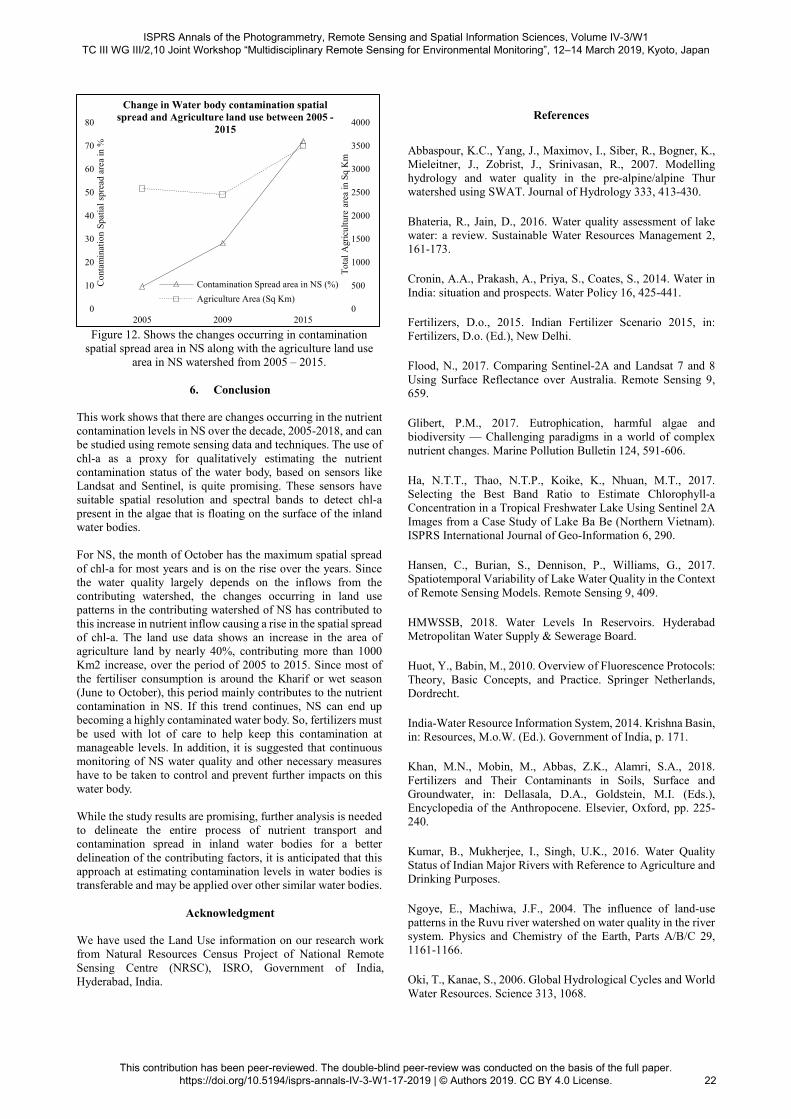
In addition, as can be seen from Figure 12, over the 10year period since 2005, the increasing agricultural land area with the corresponding increase in the fertiliser input in these lands (as discussed in the earlier paragraph) seems to the be directly responsible for the raise in the contamination levels of the water body. As most of the contributing watershed follows the Kharif croppping season, it is observed that the major inflow of the nutrient contaminants are during this season, leading to the maximum spatial spread in the month of October. Thus, the increasing agriculture land use in the wet season along with increased fertilizer usage during Kharif season have contributed largely to the increase of nutrient contamination levels in NS. The surface runoffs during the monsoon season (June to October) carry most of the nutrient contents into the water body. Hence, we can see large spatial spread of algal populations on the water surface during the month of October when compared to the other months. If this trend carries on, the NS will become highly contaminated water body. So, fertilizers must be used with lot of care to reduce the contamination levels in the NS. Along with this, continuous monitoring of NS water quality and necessary measures have to be taken to prevent further damage.
Figure 10: Shows the amount of monthly Urea usage in
Telangana State, where NS is situated, for the year 2015 and also the volume of water in NS in TMC from 2015 – 2018.
Figure 11: Shows the increase in the Nitrogen, Phosphorus and
Potassium usage in India from 1951 – 2015.
23 30 22 24
4831
25 19 26 240
17
29 29 29 29 29 30
16 15 16 15 14 146 6 6 6 6 6
1 2 2 2 2 2
2005 2007 2009 2011 2013 2015
Change in Land Use area (%) in NS contributing watershed
Buit up area Water bodiesWaste land Decidious forestFallow land Agriculture
2582
3357
2453 26
35
4392
3493
311
221
760
201
147
226
1799 22
00
1098
2197
3739
2895
428
893
551
194 46
3
324
2005 2007 2009 2011 2013 2015
Agriculture Land area (Sq Km) in various cropping seasons in NS Watershed
Total Agriculture land Rabi Kharif Double/Triple Crop
12%
7%
31%
8%
3% 6%
70%
66%
45%
83%
85%
83%
17%
27%
22%
7% 11%
9%
2005 2007 2009 2011 2013 2015
Agriculture Land area (%) in various cropping seasons in NS Watershed
Rabi Kharif Double/Triple Crop
7162
6
1335
53
1403
89
9238
3
8269
4
9884
4
1514
05
1590
62
1653
44
9852
9
5095
0
6616
5
0
50
100
150
200
250
300
350
0
50000
100000
150000
200000Ja
n
Feb
Mar
Apr
May Jun
Jul
Aug Sep
Oct
Nov Dec
TMC
Tonn
es2015 Monthwise Urea Usage in Telangana
2015 Urea Usage in Telangana (Tonnes)Volume of water in NS in 2015Volume of water In NS in 2016Volume of water in NS in 2017Volume of water in NS in 2018
0
2000
4000
6000
8000
10000
12000
14000
16000
18000
20000
1950
-51
1960
-61
1970
-71
1980
-81
1986
-87
1988
-89
1990
-91
1992
-93
1994
-95
1996
-97
1998
-99
2000
-01
2002
-03
2004
-05
2006
-07
2008
-09
2010
-11
2012
-13
2014
-15
Thou
sand
s of
Ton
nes
All India Consumption of Fertilizers (1951-2015)
NitrogenPhosphorusPotassium
A
B
ISPRS Annals of the Photogrammetry, Remote Sensing and Spatial Information Sciences, Volume IV-3/W1 TC III WG III/2,10 Joint Workshop “Multidisciplinary Remote Sensing for Environmental Monitoring”, 12–14 March 2019, Kyoto, Japan
Figure 12. Shows the changes occurring in contamination
spatial spread area in NS along with the agriculture land use area in NS watershed from 2005 – 2015.
6. Conclusion
This work shows that there are changes occurring in the nutrient contamination levels in NS over the decade, 2005-2018, and can be studied using remote sensing data and techniques. The use of chl-a as a proxy for qualitatively estimating the nutrient contamination status of the water body, based on sensors like Landsat and Sentinel, is quite promising. These sensors have suitable spatial resolution and spectral bands to detect chl-a present in the algae that is floating on the surface of the inland water bodies. For NS, the month of October has the maximum spatial spread of chl-a for most years and is on the rise over the years. Since the water quality largely depends on the inflows from the contributing watershed, the changes occurring in land use patterns in the contributing watershed of NS has contributed to this increase in nutrient inflow causing a rise in the spatial spread of chl-a. The land use data shows an increase in the area of agriculture land by nearly 40%, contributing more than 1000 Km2 increase, over the period of 2005 to 2015. Since most of the fertiliser consumption is around the Kharif or wet season (June to October), this period mainly contributes to the nutrient contamination in NS. If this trend continues, NS can end up becoming a highly contaminated water body. So, fertilizers must be used with lot of care to help keep this contamination at manageable levels. In addition, it is suggested that continuous monitoring of NS water quality and other necessary measures have to be taken to control and prevent further impacts on this water body. While the study results are promising, further analysis is needed to delineate the entire process of nutrient transport and contamination spread in inland water bodies for a better delineation of the contributing factors, it is anticipated that this approach at estimating contamination levels in water bodies is transferable and may be applied over other similar water bodies.
Acknowledgment We have used the Land Use information on our research work from Natural Resources Census Project of National Remote Sensing Centre (NRSC), ISRO, Government of India, Hyderabad, India.
References
Abbaspour, K.C., Yang, J., Maximov, I., Siber, R., Bogner, K., Mieleitner, J., Zobrist, J., Srinivasan, R., 2007. Modelling hydrology and water quality in the pre-alpine/alpine Thur watershed using SWAT. Journal of Hydrology 333, 413-430.
Bhateria, R., Jain, D., 2016. Water quality assessment of lake water: a review. Sustainable Water Resources Management 2, 161-173.
Cronin, A.A., Prakash, A., Priya, S., Coates, S., 2014. Water in India: situation and prospects. Water Policy 16, 425-441.
Fertilizers, D.o., 2015. Indian Fertilizer Scenario 2015, in: Fertilizers, D.o. (Ed.), New Delhi.
Flood, N., 2017. Comparing Sentinel-2A and Landsat 7 and 8 Using Surface Reflectance over Australia. Remote Sensing 9, 659.
Glibert, P.M., 2017. Eutrophication, harmful algae and biodiversity — Challenging paradigms in a world of complex nutrient changes. Marine Pollution Bulletin 124, 591-606.
Ha, N.T.T., Thao, N.T.P., Koike, K., Nhuan, M.T., 2017. Selecting the Best Band Ratio to Estimate Chlorophyll-a Concentration in a Tropical Freshwater Lake Using Sentinel 2A Images from a Case Study of Lake Ba Be (Northern Vietnam). ISPRS International Journal of Geo-Information 6, 290.
Hansen, C., Burian, S., Dennison, P., Williams, G., 2017. Spatiotemporal Variability of Lake Water Quality in the Context of Remote Sensing Models. Remote Sensing 9, 409.
HMWSSB, 2018. Water Levels In Reservoirs. Hyderabad Metropolitan Water Supply & Sewerage Board.
Huot, Y., Babin, M., 2010. Overview of Fluorescence Protocols: Theory, Basic Concepts, and Practice. Springer Netherlands, Dordrecht.
India-Water Resource Information System, 2014. Krishna Basin, in: Resources, M.o.W. (Ed.). Government of India, p. 171.
Khan, M.N., Mobin, M., Abbas, Z.K., Alamri, S.A., 2018. Fertilizers and Their Contaminants in Soils, Surface and Groundwater, in: Dellasala, D.A., Goldstein, M.I. (Eds.), Encyclopedia of the Anthropocene. Elsevier, Oxford, pp. 225-240.
Kumar, B., Mukherjee, I., Singh, U.K., 2016. Water Quality Status of Indian Major Rivers with Reference to Agriculture and Drinking Purposes.
Ngoye, E., Machiwa, J.F., 2004. The influence of land-use patterns in the Ruvu river watershed on water quality in the river system. Physics and Chemistry of the Earth, Parts A/B/C 29, 1161-1166.
Oki, T., Kanae, S., 2006. Global Hydrological Cycles and World Water Resources. Science 313, 1068.
0
500
1000
1500
2000
2500
3000
3500
4000
2005 2009 20150
10
20
30
40
50
60
70
80
Tota
l Agr
icul
ture
are
a in
Sq
Km
Con
tam
inat
ion
Spat
ial s
prea
d ar
ea in
%Change in Water body contamination spatial
spread and Agriculture land use between 2005 -2015
Contamination Spread area in NS (%)Agriculture Area (Sq Km)
ISPRS Annals of the Photogrammetry, Remote Sensing and Spatial Information Sciences, Volume IV-3/W1 TC III WG III/2,10 Joint Workshop “Multidisciplinary Remote Sensing for Environmental Monitoring”, 12–14 March 2019, Kyoto, Japan
Olmanson, L.G., Brezonik, P.L., Bauer, M.E., 2011. Evaluation of medium to low resolution satellite imagery for regional lake water quality assessments. Water Resources Research 47, n/a-n/a.
Prasanna, V., 2014. Impact of monsoon rainfall on the total foodgrain yield over India. Journal of Earth System Science 123, 1129-1145.
Salem, S.I., Higa, H., Kim, H., Kobayashi, H., Oki, K., Oki, T., 2017. Assessment of Chlorophyll-a Algorithms Considering Different Trophic Statuses and Optimal Bands. Sensors (Basel, Switzerland) 17, 1746.
Satistics, D.o.E.a., 2017. Pocket Book of Agricultural Statistics, 2017, in: Department of Agriculture, C.a.F.W. (Ed.), New Delhi.
Sharma, B.R., Rao, K.V., Vittal, K.P.R., Ramakrishna, Y.S., Amarasinghe, U., 2010. Estimating the potential of rainfed agriculture in India: Prospects for water productivity improvements. Agricultural Water Management 97, 23-30.
Sharma, R.K., Yadav, M., Gupta, R., 2017. Chapter Five - Water Quality and Sustainability in India: Challenges and Opportunities, in: Ahuja, S. (Ed.), Chemistry and Water. Elsevier, pp. 183-205.
Smith, V.H., Schindler, D.W., 2009. Eutrophication science: where do we go from here? Trends in Ecology & Evolution 24, 201-207.
Smith, V.H., Tilman, G.D., Nekola, J.C., 1999. Eutrophication: impacts of excess nutrient inputs on freshwater, marine, and terrestrial ecosystems. Environmental Pollution 100, 179-196.
Tan, W., Liu, P., Liu, Y., Yang, S., Feng, S., 2017. A 30-Year Assessment of Phytoplankton Blooms in Erhai Lake Using Landsat Imagery: 1987 to 2016. Remote Sensing 9, 1265.
Tarun Teja, K., Rajan, K.S., 2016. Understanding the behaviour of contamination spread in Nagarjuna Sagar reservoir using temporal Landsat data. Int. Arch. Photogramm. Remote Sens. Spatial Inf. Sci. XLI-B8, 343-348.
Tewatia, R.K., Chanda, T.K., 2017. 4 - Trends in Fertilizer Nitrogen Production and Consumption in India, in: Abrol, Y.P., Adhya, T.K., Aneja, V.P., Raghuram, N., Pathak, H., Kulshrestha, U., Sharma, C., Singh, B. (Eds.), The Indian Nitrogen Assessment. Elsevier, pp. 45-56.
ISPRS Annals of the Photogrammetry, Remote Sensing and Spatial Information Sciences, Volume IV-3/W1 TC III WG III/2,10 Joint Workshop “Multidisciplinary Remote Sensing for Environmental Monitoring”, 12–14 March 2019, Kyoto, Japan