Page 1
1
NGENE, AMUCHE NNENNA
PG/MSC/07/43243
EXCHANGE RATE FLUCTUATIONS AND TRADE FLOWS IN
NIGERIA: A TIME SERIES ECONOMETRIC MODEL
Economics
AN MSC PROJECT RESEARCH SUBMITTED TO THE DEPARTMENT
OF ECONOMICS, FACULTY OF THE SOCIAL SCIENCES, UNIVERSITY OF NIGERIA, NSUKKA
Webmaster
2010
UNIVERSITY OF NIGERIA
Page 2
2
EXCHANGE RATE FLUCTUATIONS AND TRADE FLOWS
IN NIGERIA: A TIME SERIES ECONOMETRIC MODEL
AN MSC PROJECT RESEARCH SUBMITTED TO THE
DEPARTMENT OF ECONOMICS, FACULTY OF THE SOCIAL
SCIENCES, UNIVERSITY OF NIGERIA, NSUKKA, IN PARTIAL
FULFILMENT OF THE REQUIREMENTS FOR THE AWARD OF
MASTER OF SCIENCE (M.SC) DEGREE IN ECONOMICS
BY
NGENE, AMUCHE NNENNA
PG/MSC/07/43243
SUPERVISOR: REV FR. DR. ICHOKU, H. E.
OCTOBER, 2010
Page 3
3
TITLE PAGE
EXCHANGE RATE FLUCTUATIONS AND TRADE FLOWS
IN NIGERIA: A TIME SERIES ECONOMETRIC MODEL
Page 4
4
CERTIFICATION
This is to certify that Ngene, Amuche Nnenna, a post-graduate student of the
Department of Economics, University of Nigeria, Nsukka, and whose registration
number is PG/M.Sc/07/43243 has satisfactorily completed the requirements for the
award of Master of Science (M.Sc) Degree in Economics.
REV FR. DR H. E. ICHOKU PROF C. C. AGU
Supervisor Head of Department
Page 5
5
APPROVAL PAGE
This project has been read and approved as meeting the requirements for the award of
the Degree of Master of Science (M.Sc) of the Department of Economics, University of
Nigeria, Nsukka.
REV FR. DR H. E. ICHOKU PROF C. C. AGU
Supervisor Head of Department
PROF E. O EZEANI
Dean, Faculty of Social Sciences External Examiner
Page 6
6
DEDICATION
To the infinite merciful God, who has proved that something good
can come out of Nazareth. Also, to my industrious and
resilient mother, for her immense sacrifice on me.
Page 7
7
ACKNOWLEDGEMENTS
Oh gracious God, great is thy faithfulness, for morning by morning thy new mercies I
beheld throughout the period of my study. I remain ever grateful.
To my resourceful project supervisor, Rev Fr. Dr. H. E. Ichoku, I say a million thanks
for your immense contributions amidst your tight schedules and fatherly advice to make
the research work a great success. Sincerely, you are a father and supervisor with a
difference.
Engr. Dr. Ben U. Ngene, I lack words to express my sincere gratitude to you. Indeed,
you are the worthy brain behind what I am, what I have achieved and whatever success I
reckon in life. I can only say thanks a million for your immense and immeasurable
supports to make my life worth it.
To my industrious and resilient mother, Mrs Theresa Ngene, I appreciate you greatly for
your unprecedented love, care and the burden you took to make my life what it is today.
Mum, I am indeed proud to have you as a parent. And to my entire siblings, your
goodwill, love and maximum support is highly appreciated.
I am highly indebted to all the lecturers in the Department of Economics, especially,
Prof(s) Agu, Ikpeze, Onah and Ogbu, Dr(s) Fonta, Onyukwu, Moses, Amuka, Dr (Mrs)
Madueme and Mr(s) Ukwueze, Urama, Chukwu J., Ugbor, etc. for their maximum
contributions to my life career. I owe special thanks to Dr (Mrs) Aneke, for giving me a
feeling of mother away from my mother. I remain most gratefully to Mr Nwosu
Emmanuel and Dr Asogwa whose academic assistance and commitment provided the
background knowledge that made the research a great success. And to all the non-
academic staff of the department, I appreciate you all for your great help.
Also, my profound gratitude goes to the staff of the CBN and National Bureau of
Statistics for their cooperation and efforts in making the data used for the study
available. Indeed, I appreciate wonderfully the inspiration, encouragement and efforts of
the following friends, roommates and classmates: Andy, Austin, Ijeoma, Samson,
Michael, Margaret, Ifeoma, Gabriel, I.k, Sir Pee, Emmanuel, Floxy, Ifeanyi, Chairmoo,
Nneka, Chineye, Kelechi, etc. Finally, to Bishop (Dr) Ken Uloh of DGLA, Nsukka and
GSF I say big thanks for being there always for me.
Ngene, Amuche
October, 2010
Page 8
8
TABLE OF CONTENTS
Page
Title Page .. .. .. i
Certification Page .. .. .. ii
Approval Page .. .. .. iii
Dedication .. .. .. iv
Acknowledgement .. .. .. v
Table of Contents .. .. .. vi
List of Tables .. .. .. viii
Abstract .. .. .. ix
CHAPTER ONE: INTRODUCTION
1.1 Background of the Study .. .. .. 1
1.2 Statement of the Problem .. .. .. 2
1.3 Research Questions .. .. .. 4
1.4 Objectives of the Study .. .. .. 4
1.5 Research Hypotheses .. .. .. 4
1.6 Significance of the Study .. .. .. 5
1.7 Scope of the Study .. .. .. 5
1.8 Summary .. .. .. 5
CHAPTER TWO: LITERATURE REVIEW
2.1 Theoretical Literature .. .. .. 6
2.2 Conceptual Issues in Exchange Rate Fluctuations .. .. .. 11
2.3 Empirical Literature .. .. .. 11
2.4 Theoretical Framework .. .. .. 14
2.5 Limitations of the Previous Studies .. .. .. 17
2.6 Summary .. .. .. 19
CHAPTER THREE: EXCHANGE RATE FLUCTUATIONS IN THE CONTEXT
OF NIGERIAN ECONOMY
3.1 Introduction .. .. .. 20
3.2 Brief Overview of Exchange Rate Regimes .. .. .. 20
Page 9
9
3.3 Historical and Current Developments of Exchange Rate Policies
in Nigeria .. .. .. 22
3.4 General Survey of Nigeria‟s Trade Policies and Performance .. 25
3.5 Trade and the Nigerian Economy .. .. .. 26
3.6 The Impact of Exchange Rate Fluctuations on Nigeria‟s Trade
and Growth .. .. .. 27
3.7 The CBN‟s Policy Responses to Exchange Rate Fluctuations in Nigeria 28
CHAPTER FOUR: RESEARCH METHODOLOGY
4.1 Analytical Framework of the Models Used .. .. .. 31
4.2 Data Transformation .. .. .. 32
4.3 Model Specification .. .. .. 33
4.4 Justification of the Models Used .. .. .. 38
4.4 Sources of Data and Variables used .. .. .. 38
4.5 Estimation Technique and Procedure .. .. .. 39
CHAPTER FIVE: DATA PRESENTATION AND DISCUSSION OF RESULTS
5.1 Interpolation of Time Series Data .. .. .. 41
5.2 Time Series Properties .. .. .. 41
5.3 Cointegration Analyses .. .. .. 44
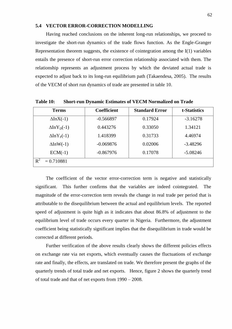
5.4 Vector Error-Correction Modelling .. .. .. 51
5.5 Variance Decomposition and Impulse Response Analyses .. .. 53
CHAPTER SIX: SUMMARY, CONCLUSION AND RECOMMENDATIONS
6.1 Summary of the Major Findings .. .. .. 57
6.2 Conclusion and Lessons for Policy Issues .. .. .. 58
6.3 Recommendations .. .. .. 60
References .. .. .. 63
Appendix
Page 10
10
LIST OF TABLES
Page
Table 1: Value of Nigeria‟s exports and imports, 1996 – 2004 .. .. 26
Table 2: Main Origins of Nigeria‟s Exports and Imports (% of total) .. 27
Table 3: Example of Interpolation of Data .. .. 41
Table 4: Unit Root Test Results .. .. 42
Table 5: Effect of Different Macroeconomic Policies on
Net Exports/Trade Balance .. .. 43
Table 6: The Engle-Granger Cointegration Tests .. .. 45
Table 7: Multivariate Johansen Cointegration Test Results .. .. 45
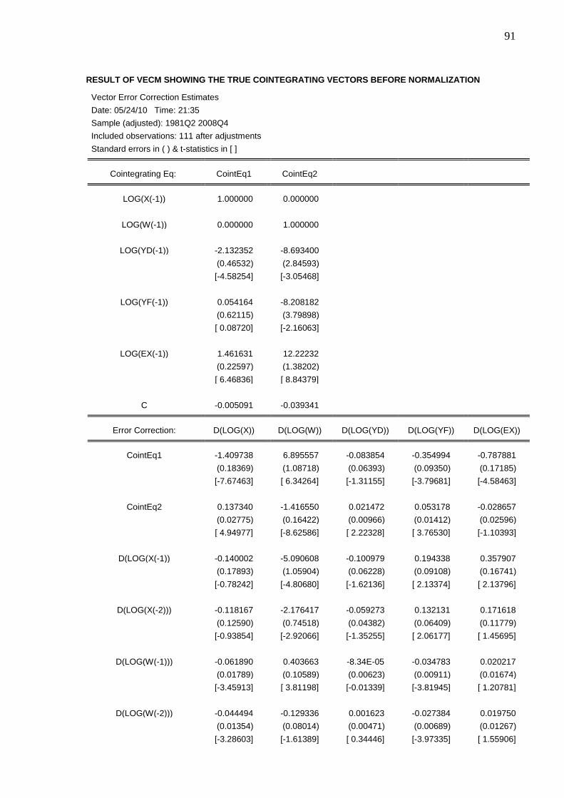
Table 8: VECM Results before Normalization, indicating the two True
Cointegrating Vectors .. .. 47
Table 9: Long-run Parameters of VECM Normalized on Trade .. 49
Table 10: Short-run Dynamic Estimates of VECM Normalized on Trade 51
Table 11: Variance Decomposition of Trade Flows (X) .. .. 54
Table 12: The Impulse Response Analysis of Trade in
Nigeria Response of LOG(X): .. .. 56
Page 11
11
ABSTRACT
Consequent upon the collapse of the Bretton Woods system and the resultant adoption of the
flexible exchange rate system in 1973, economists and policy-makers have been concerned
about the significant effects of exchange rate fluctuations on the economy in general and
trade, in particular. However, theoretical and empirical works on the subject have produced
mixed results. This study investigates exchange rate fluctuations and trade flows in Nigeria:
A time-series econometric model for the period 1980:1 to 2008:4, using GARCH modelling,
Mundell-Fleming model, multivariate Johansen cointegration test, vector error-correction
mechanism, and complemented by variance decomposition and impulse response analyses.
Empirically, interesting results were found. Exchange rate fluctuations are found to have a
negative and significant effect on Nigeria’s trade with the US. Different policy changes in
the economy are found to have great influence on the fluctuations of exchange rate, which
directly or indirectly affect trade flows negatively. In line with theoretical expectation, US
GDP exerts a significant positive effect on Nigeria’s trade but curiously, domestic income
exerts a significant negative effect on trade. The study also revealed that real exchange rate
may lead to an increase in the volume of net exports. Hence, policy-makers seeking export
promotion (import prohibition) strategies can use the real exchange rate as a means of
boosting trade. However, any exchange rate policy in the country that aims to encourage
trade regardless of its fluctuations is likely to be counterproductive. It is instructive
therefore, for policymakers to work towards increasing Nigeria’s trade while ensuring a
stable exchange rate that will equally not stabilize poverty.
Page 12
12
CHAPTER ONE
INTRODUCTION
1.1 BACKGROUND OF THE STUDY
Risk in international commodity trade usually emanates from two main sources:
changes in world prices or fluctuations in exchange rate. Consequent upon the collapse
of the Bretton Woods system and the resultant adoption of the flexible exchange rate
system in 1973, economists and policy makers have been concerned about the
significant effects of exchange rate fluctuations on the economy in general and trade, in
particular (Isitua & Neville: 2006). One of the most dramatic events in Nigeria over the
past decade was the devaluation of the Nigerian naira with the adoption of a structural
adjustment programme (SAP) in 1986. A cardinal objective of the SAP was the
restructuring of the production base of the economy with a positive bias for the
production of agricultural exports. The foreign exchange reforms that facilitated a
cumulative depreciation of the effective exchange rate were expected to increase the
domestic prices of agricultural exports and hence boost domestic production.
Significantly, this depreciation resulted in changes in the structure and volume of
Nigeria‟s exports as determined empirically by many researchers (Oyejide: 1986,
Ihimodu: 1993 and World bank: 1994). The depreciation increased the prices of
agricultural exports and the result indicated a marked increase in the volume of
agricultural exports over the years.
The two major strands of argument in the literature regarding the actual
relationship between exchange rate fluctuations and trade flows are between the
traditional and the risk-portfolio schools. The traditional school is of the opinion that
exchange rate fluctuations have negative effects on multilateral, bilateral and sectoral
trade. Higher exchange rate fluctuations lead to higher costs, risk and uncertainty of
profit in international transactions, economic agents as a result, respond by favouring
domestic-foreign trade just at the margin, hence, it reduces or depress the volume of
trade (Clark: 1973, Chowdhury: 1993, Cushman: 1983, 1988, Kenen & Rodrik: 1986,
etc). The second strand, which is the risk-portfolio school, argues that economic agents
in international transactions maximize their profits by diversifying the risk levels of their
portfolio, and as such, higher exchange rate fluctuations with the resulting higher risk
would not discourage them from engaging in trade but rather would present an
Page 13
13
opportunity for them to diversify their risk portfolios from high risk portfolio to low and
medium risk portfolio and still increase their profit. In other words, exchange rate
fluctuations promote the volume of trade (De Grauwe: 1988, IMF: 1984, Klein: 1990,
and Chambers, et al: 1991).
It became a source of concern to both the economists and policy makers that
despite the existence of literature on the issue, theoretical and empirical works on the
subject are yet to produce a consensus. And although these studies are very important
for policy reasons, only few attempts have been made to examine them for developing
countries, Nigeria inclusive. The available instances include Vergil (2002) for Turkey
and Bah and Amusa (2003) and Takaendesa, et al (2005) for South Africa, Ajayi (1988),
Adubi, et al (1999), Osagie (1985), Isitua and Neville (2006), and Osuntogun, et al
(1993) for Nigeria.
1.2 STATEMENT OF THE PROBLEM
Fluctuations in the exchange rate movements since the beginning of the floating
exchange rate regime have raised concerns particularly on the impact of such
movements on trade flows. Fluctuation is a major constraint on development of an
economy, making planning more problematic and investment more risky. For instance,
if potential foreign investors to Nigeria are risk averse (or even risk neutral), larger
exchange rate fluctuations may reduce the overall foreign direct investment inflows
since it increases uncertainty over the returns in a given investment. Potential investors
will invest in a foreign location only if the expected returns are high enough to cover for
the currency risk (Gerardo, et al: 2002).
Most developing economies are net debtors and in consequence, changes in the
trading partners‟ exchange rates may affect the real cost of servicing their debts. A
strong appreciation of the dollar, for example, implies a higher cost of servicing an
external debt that is mainly denominated. Furthermore, for a developing country like
Nigeria that is highly dependent on trade, the exchange rate, which is the price of foreign
exchange, has implications for balance of payments viability and the level of external
debt. For instance, if the exchange rate is overvalued, then it would result to
unsustainable balance of payments deficit, encourage capital flight and escalate external
debt stock, which in turn will lead to declining level of investment. On the other hand, a
real depreciation raises the cost of imported capital goods, and since a large chunk of
investment goods in developing countries is imported, domestic investment would be
Page 14
14
expected to fall with a real depreciation (Iyoha, 1998). All these show that the impact
of exchange rate variability on economies especially developing ones is not only in one
direction.
Therefore, understanding the behaviour of the exchange rate is very important for
many reasons. First, the relationship between a country‟s exchange rate and economic
growth via trade is a crucial issue from both the descriptive and policy prescription
perspectives. As Edwards (1994:61) asserts: “It is not an overstatement to say that the
issue of real exchange rate behaviour now occupies a central role in policy evaluation
and design”. A country‟s exchange rate behaviour is an important determinant of the
growth of its cross-border trading and it serves as a measure of its international
competitiveness (Bah and Amusa: 2003). It also plays a crucial role in guiding the
broad allocation of production and spending between foreign and domestic goods. In
addition, researches have shown that exchange rate stability influences importantly
export growth, consumption, resource allocation, employment and private investments
(Takaendesa, et al: 2005, Aron et al, 1999). The behaviour of exchange rate is a useful
indicator of economic performance of an economy that needs to be understood. In other
words, assessing the link between exchange rate fluctuations and Nigeria‟s trade flows
would have policy implication. Also, variability of the naira value in recent years calls
for understanding of the factors that actually cause exchange rate to fluctuate. For
example, knowledge of these would help to facilitate policies that would aid the
attainment of exchange rate stability and economic growth through trade flows in the
long run.
Furthermore, along the lines of the existing literature, a related question very few
researchers have investigated is whether changes in exchange rate regimes or policies
which can be associated with a shift in the amplitude of fluctuations cause export flows
to decrease. Few others, for reasons known to them, ascertained the impact of these
fluctuations on either the oil sector, excluding the non-oil sector or vice versa.
Nevertheless, we know that in a country like Nigeria that is so much over-dependent on
oil, assessing the effect of exchange rate fluctuations on either oil or non-oil sector trade
exclusively may not really give a value judgement and the conclusion thereof.
However, to bridge this gap and also avoid the effect of Dutch disease associated
with some previous findings, the current study attempts to examine the possible effect
and link between exchange rate fluctuations and Nigeria‟s trade flows for both the oil
and the non-oil sectors.
Page 15
15
Finally, the study covers longer period more than any of the previous studies,
which is, 1980 – 2008, the time span of the previous studies were too brief to capture the
long-run effects of fluctuations on trade. Hence, our results are therefore likely to be
more reliable for policy purposes.
1.3 RESEARCH QUESTIONS
In view of the above problems, the following research questions are raised:
1. What are the effects of different macroeconomic policies on exchange rate in
Nigeria?
2. What is the level of exchange rate fluctuations transmission to trade flows
(exports and imports) variability in Nigeria?
3. Does any long-run linear combination of cointegrating vectors of trade and
exchange rate fluctuations exist and the short-run dynamic adjustment process by
which trade could converge on its equilibrium position in Nigeria?
1.4 OBJECTIVES OF THE STUDY
The overall objective of the study is to examine empirically the link between
exchange rate fluctuations and Nigeria‟s trade flows (oil and non-oil trade) by first
determining the effect of different policy frameworks on exchange rate.
Specifically the study intends to:
Determine the effect of different policy framework on exchange rate in Nigeria.
Ascertain the transmission level of exchange rate fluctuations on exports and
imports (trade) variability in Nigeria.
Assess the long-run linear combination of cointegrating vectors of trade and
exchange rate fluctuations and the short-run dynamic adjustment process by
which trade could converge on its equilibrium position in Nigeria.
1.5 RESEARCH HYPOTHESES
The following research null hypotheses are tested
Different macroeconomic policy framework applied do not significantly affect
Nigeria‟s exchange rate.
Exchange rate fluctuations do not transmit significantly on exports and imports
variability in Nigeria.
Page 16
16
There is no significant long-run linear combination of cointegrating vectors of
trade flows and exchange rate fluctuations in Nigeria.
1.6 SIGNIFICANCE/POLICY RELEVANCE OF THE STUDY
The study is of relevance to the Nigerian economy in the following ways:
It serves as a future guide to the policy makers in the formulation of better and
efficient policy options for managing exchange rate fluctuations in Nigeria. Also, the
research is of immense help to the general economy, as it provides possible measures
that monetary authority could adopt in order to maintain stability in exchange rate so
that, it can influence importantly export growth, consumption, resource allocation,
employment and private and foreign investments as research has shown. Above all, it
adds to the existing literature thus, provides relevant information that could guide further
researchers on the subject.
1.7 SCOPE OF THE STUDY
The discussions in this work are based on the macroeconomic issue (exchange rate
fluctuations) affecting Nigerian economy in the growth of its cross-border trading and
international competitiveness. Hence, the study is limited to the Nigerian economy for
the period covered, which is 1980 – 2008. This range is chosen to ensure availability of
data and for the analysis to be meaningful and aid in the achievement of the objectives
of the work.
1.8 SUMMARY
In the foregoing, we have tried to set out the research problems, motivation and
objectives of the study.
In the next section, the theoretical and empirical literature is reviewed to provide a
link between theory, previous documented evidence and what this work intends to
achieve.
Page 17
17
CHAPTER TWO
LITERATURE REVIEW
2.1 THEORETICAL LITERATURE
Since the adoption of floating exchange rate in the developing countries in 1973,
the question of whether exchange rate changes/uncertainty have independent adverse
effects on exports and trade has attracted a lot of attention in the literature. The
introduction of Structural Adjustment Programmes by many of these countries and the
attendant liberalization of exchange rates has brought the discussion of this issue further
into global focus. A review of the literature shows that the issue is far from being
settled, though not all studies are fully comparable.
There are two major trends of argument in the literature. The first argues that
exchange rate fluctuations will impose costs on risk-averse market participants who will
generally respond by favouring domestic to foreign trade at the margin. Early study of
this issue focused on firm‟s behaviour and presumed that increased exchange rate
fluctuations would increase the uncertainty of profits on contracts denominated in a
foreign currency and would therefore reduce international trade to level lower than
would otherwise exist if uncertainty were removed. This uncertainty of profits, or risk,
would lead risk-averse and risk-neutral agents to redirect their activity from higher-risk
foreign markets to the lower risk home market.
Clark (1973) study, in many ways lays the theoretical groundwork for the
traditional school by examining bilateral trade and the behaviour of risk-averse firms.
Numerous restrictions are imposed, including firms that only produce goods for exports,
limited hedging possibilities, contracts denominated in foreign currencies, no imported
factor inputs and a perfectly competitive marketplace. He supposes that as the variance
of exchange rate uncertainty increases, so does the uncertainty of profitability, where
profits are expressed in the home currency. Utility is given as a quadratic function of
profits ))(( 2 baU , where b as a risk aversion parameter, is less than zero. As
uncertainty increases, Clark contends, that a risk-averse firm will reduce the supply of
goods to the level where marginal revenue actually exceeds marginal cost in order to
compensate for the additional risk, thereby maximizing utility.
Page 18
18
The argument views traders as bearing undiversified exchange risk; if hedging is
impossible or costly and traders are risk-averse or even risk neutral, risk-adjusted
expected profits from trade will fall when exchange risk increase (Chowdhury: 1993).
Also, Qian and Varangis (1992) assert that exchange rate fluctuations increase the
risk and uncertainty in international transactions and thus discourage trade; if traders are
risk averse, they will be willing to incur an added cost to avoid the risk associated with
the exchange rate fluctuations. Thus, a firm‟s export supply (import demand) curve will
shift to the left (right) in the presence of exchange rate fluctuations; for any quantity of
exports or imports, the corresponding price will be higher under exchange rate
fluctuations or risk than without it.
Another traditional school examination of fluctuations and bilateral trade is that of
Hooper and Kohlhagen (1978). They derive demand and supply schedules for individual
firms, where the explanatory variables include the currency denomination of contracts,
the degree of firms‟ risk aversion and the percentage of risk hedged in the forward
market. Perhaps the most significant contribution of this study is how it allows nominal
exchange rate volatility to only impact the amount of risk that remains unhedged. Their
study involved a number of a priori assumptions, including the importer being a price-
taker (where imports are assumed to be inputs used for producing goods that are sold
domestically), the importer facing a known demand curve and exporters that sell all of
their products abroad in a monopolistic market framework. They found that increased
exchange rate fluctuations lead to both downward-shifting supply and demand curves,
where quantities and prices decline when importers face the exchange rate risk
(depending on demand elasticity and their degree of risk-aversion), and quantities
decline and prices increase when exporters (suppliers) bear the risk.
Other studies in support of this idea include: Chusman (1983, 1988), Kenen and
Rodrik (1986), Kroner and Lastrapes (1991), Thursby and Thursby (1987), Akhtar and
Hilton (1984), and Isitua and Neville (2006). In other words, their studies indicate a
significant depressive effect of exchange risk on international trade.
Some studies such as Caballero and Corbo (1989), Kumar and Dhawan (1991),
concluded that due to the political economy, effects of exchange rate fluctuations, its
increase was responsible for the slowdown in trade in the 1970s. In essence, the flexible
exchange rate led to misalignments of major currencies, which led in turn, to adjustment
problems in the tradable goods sector and political pressures toward protectionism.
Page 19
19
Côté, (1994), in her comprehensive review of the literature, pointed out that the
traditional school (theories that exchange rate fluctuations affects trade negatively) has
examined not only the presence of risk, but also its degree, which in turn depends upon
such factors as whether production inputs are imported, the opportunity to hedge risk
and the currency in which contracts are denominated.
One of the main objections to the traditional school is that it does not properly
model how firms manage risk, not only through the use of derivatives, but also as an
opportunity to increase profitability. For this reason the argument turns to the risk-
portfolio school. What is referred to here as the risk-portfolio school is not a unified
body of thought, but is comprised rather of multiple theories, varying in complexity, but
united in the opinion of the traditional school as unrealistic.
This second strand of the literature argues that traders benefit from exchange rate
fluctuations or risk. According to these studies, trade can be considered as an option
held by firms - like any other options, such as stocks, the option value of trade can rise
with fluctuations Bredin, et al (2003).
De Grauwe (1988), in a straight forward attack on the former school, convincingly
argues that due to the convexity of the profit function, exporters‟ return from favourable
exchange rate movements and the accompanying increased output outstrip the decreased
profits associated with adverse exchange rates and decreased output, and therefore: “As
a result, risk-neutral individuals would be attracted by these higher profit opportunities”.
Although the convexity of the profit function may imply a positive correlation between
trade and exchange rate risk, the more prominent tenet of the risk-portfolio school
examines exchange rate risk in light of modern portfolio diversification theory.
As summarized by Farrell, et al (1983), economic agents maximize profitability by
diversifying the risk levels in their investment portfolios by simultaneously engaging in
low, medium and high-risk activity with corresponding potential rates of return. Greater
exchange rate fluctuations resulting in higher risk would then not discourage risk-neutral
agents from engaging in trade, but would present an opportunity to diversify their risk
portfolios and increase the likelihood of profitability.
Frankel (1991) argues that if exporters are sufficiently risk-averse, an increase in
exchange rate fluctuations may result in an increase in the expected marginal utility of
export revenue which serves as incentive to exporters to increase their exports in order
to maximize their revenues.
Page 20
20
Dellas and Zilberfarb (1993), examine trade decisions in the framework of a
portfolio-savings decision model under uncertainty. Their theoretical model assumes a
small open economy with an individual domestic agent importing, exporting and
consuming two products in two time periods, where asset markets are incomplete and
the agent makes trade decisions with incomplete knowledge of price risk. Their study
examines the effects of uncertainty both in the absence of a forward market and with
complete and incomplete hedging opportunities. Without a forward exchange market,
the individual maximizes utility by choosing a quantity of exports X such that:
),( PXXYEuq
where XY is the consumption of the exportable good and P is the real exchange
rate, with first order condition: 0)( 21 PuuE .
The effect of increased exchange rate fluctuations on trade depends on whether the
function 12 UPug is concave or convex, which in turn is determined by a degree of
risk-aversion in the utility function. With a forward exchange market, the domestic agent
maximizes utility, ),( 21 CCEu , subject to the constraints:
2111 XXYC
22112 XPXPC
With two products and incomplete forward market opportunities ( 1X representing
an exportable good subject to risk and 2X completely hedged), they find that the effects
of fluctuations on trade are ambiguous depending on the risk parameter a . With
complete hedging possible and costless, individuals can insulate themselves from
exchange rate risk and increased fluctuations do not depress trade levels. They then
extend these findings to producers selling to both domestic and foreign markets and find
results consistent with those for the individual domestic agent.
Broll and Eckwert (1999) theoretical model demonstrates how higher exchange
rate fluctuations increase the potential gains from trade. Their study uses an international
firm that sells its product either entirely at home or abroad, and must also determine
which market to choose with incomplete knowledge of exchange rate fluctuations. Their
theoretical construct results in a generally positive relationship between the variance of
the foreign spot exchange rate and the volume of output and total export. As with Dellas
and Zilberfarb, the increase in the value of the firm‟s option to export depends on the
convexity of the relationship between profits and the exchange rate, and ultimately upon
the degree of the firm‟s risks aversion.
Page 21
21
2.1.1 Alternatives
De Grauwe suggests a third, political-economic theory. This approach proposes
that nations that have flexible exchange rate systems and experience exchange rate
misalignments are susceptible to lobbying from failing industries to create or increase
protection from trade. As a result, greater exchange rate fluctuations would decrease
trade flows as a result of protectionist legislation or executive order. Critics of this
approach, such as Côté, point out that:
i. an industry‟s vulnerability due to adverse exchange rates often reflect deeper
competitiveness issues and;
ii. flexible rates help absorb the output and unemployment costs of misalignments.
These counter-arguments speak more to the welfare effects of De Grauwe‟s theory
than to its validity. It is not difficult to produce modern examples of U.S. industries,
even those industries suffering from non-exchange rate induced competitiveness
problems, e.g. steel, that have successfully lobbied the federal government to increase
tariffs on imports whose prices were argued to be artificially low. That firms
successfully lobby governments to restrict imports (trade) is evident.
A more salient problem with De Grauwe‟s political-economic theory is how to quantify
the degree of misalignment and the resulting effects of exchange rate induced lobbying
on trade flows.
Other supporters of this argument include: IMF (1984), Chambers and Just (1991),
and Klein (1990). Their studies indicate that exchange rate fluctuations catalyse trade
flows.
Côté likened this approach to derivative markets, where trade is viewed as an
option that becomes more valuable as the exchange rate becomes more volatile.
Abel (1983) showed that if one assumes perfect competition, convex and
symmetric costs of adjusting capital, and risk neutrality, investment is a direct function
of price (exchange rate) uncertainty.
Others found no evidence to suggest that exchange rate fluctuations have any
significant impact on trade; e.g. Aristotelous (2001). Given today's well-developed
financial markets, one may argue that traders (at least to some extent) should be able to
reduce or hedge uncertainty associated with exchange rate volatility. The relationship
between exchange rate volatility and trade may then be weak, if not completely absent.
Page 22
22
McKenzie (1999) gave a thorough review of the literature and discussed several
empirical issues that may be important when determining the impact of exchange rate
fluctuations on trade. These issues are mainly related to which exchange rate
fluctuations measure to use, which sample period to consider, which countries to study,
which data frequency and aggregation level to employ and which estimation method to
apply in each specific study at hand. As pointed out by him, each of these issues and
how they are handled may be part of the explanations for the inconclusive findings in
the literature.
2.2 CONCEPTUAL ISSUES IN EXCHANGE RATE FLUCTUATIONS
Risk in international commodity trade usually emanates from two main sources:
changes in world prices or fluctuations in exchange rates. These may affect trade by
increasing the uncertainties of trade or effecting a change in the cost of transaction,
processing, etc. The state of the two major sources determines the eventual domestic
trade price of a commodity over a period of time. In other words, a decision to produce
for exports involves uncertainties about the prices in the foreign exchange that such sales
will realize, as well as the exchange rate at which foreign exchange receipts can be
converted into domestic currency. In a period of fixed exchange rates, the major source
of concern in international trade for developing countries is the fluctuations that may
arise from the world prices of primary commodities, which constitute the bulk of exports
of these countries (Adubi, et al: 1999). With the increasing embrace of the structural
adjustment programmes that have devaluation of currency or market determination of
exchange rate and all prices as the fulcrum, the attention has shifted to the fortunes of
the currencies at the foreign exchange market. Given the erratic pattern of the exchange
rate in most developing countries as a result of devaluation, there has been increasing
concern about the possible effects of exchange rate fluctuations on trade. In other
words, for international traders with a given price, the major source of uncertainty is the
exchange rate at which they can translate their sales revenue in foreign currency into
local currency.
2.3 EMPIRICAL LITERATURE
Since theory has been unable to provide a definite answer as to whether the trade
enhancing effects of portfolio diversification outweigh the costs to risk-averse economic
agents as exchange rate fluctuations increase, a deal of recent research has been devoted
Page 23
23
to empirical analysis of this issue. However, the empirical evidence on this point is still
inconclusive. The studies by Cushman (1983, 1988), Thursby and Thursby (1987),
Kenen and Rodrik (1986), Caballero and Corbo (1989), Akhtar and Hilton (1984), etc
found statistically significant evidence that exchange rate fluctuations does impede
trade. Contrarily, the results from studies by IMF (1984), Bailey and Tavlas (1988),
Frankel (1991), etc could not find conclusive evidence that exchange rate fluctuations
have had statistically significant deterrent effects on trade. Even in this latter group of
studies, the results are inconsistent across countries; results from Kroner and Lastrapes
(1991) also indicate that for some countries, exchange rate fluctuations have a negative
effect on trade but for others it does not.
Maskus (1986), however, provided a link between his study and previous works by
comparing the effects of exchange rate risk across major sectors of an economy, e.g.,
manufactured goods, agriculture, chemicals and others. He found that aggregate
bilateral agricultural trade (the United States and its major western trading partners) is
particularly sensitive to exchange rate uncertainty. Maskus argued that agriculture,
compared with manufactured goods trade, is more responsive to exchange rate changes
because (a) agricultural trade is relatively open to international trade (where openness is
measured by the ratio of exports and imports to domestic agricultural output), and (b)
agriculture exhibits a low level of industry concentration.
Arize et al. (2000) provided evidence that increased exchange rate fluctuations
have an adverse effect on trade due to risk-averse traders. That is, higher exchange rate
fluctuations lead to higher costs for risk-averse traders and thus to less volume of trade.
Baron (1976) study, also looks at bilateral trade, but focuses on how the choice of
invoicing currency affects an exporting firm‟s production and pricing decisions when
exchange rates are volatile and the marketplace is not perfectly competitive. He shows
that exporting firms face greater price risk when invoices are denominated in the foreign
currency and face greater quantity demand risk when the home currency is used. In
response, as exchange rate uncertainty increases, risk-averse, profit-maximizing firms
will increase prices when the foreign currency is used to invoice goods. Baron argues
that the way in which a firm maximizes utility (minimizes risk) when the home currency
is used for invoicing depends on the shape of the demand curve it faces: e.g., reducing
prices when demand is linear, thereby increasing demand and decreasing profit variance
(uncertainty).
Page 24
24
Philippe, et al (2006), in their studies of exchange rate fluctuations and
productivity growth: the role of financial development, offer empirical evidence that real
exchange rate volatility can have a significant impact on long term rate of productivity
growth, but the effect depends critically on a country‟s level of financial development.
Thus, countries with relatively low levels of financial development, exchange rate
fluctuations generally reduce growth, whereas for financially advanced countries, there
is no significant effect.
In Nigeria, Ajayi (1988) and Osagie (1985) using the structuralist approach in their
study of external trade flows, opposed the adoption of a more flexible exchange rate
policy in Nigeria. Their arguments were based on the fact that exchange rate
devaluation would be stagflationary and have no significant effects on the external trade
balance in the less developed countries because of the low price elasticity generally
associated with the excess import and export demand functions.
The findings of Ajayi (1988) and Osagie (1985) support an earlier study by Ojo
(1978) who suggested that exchange rate changes need not play any significant role in
the explanation of Nigerian import-export balance.
Adubi, et al (1999), in their studies of price, exchange rate volatility and Nigeria‟s
agricultural trade flows, argue that if the exchange rate change is more volatile, it tends
to increase the prices of export crops, but the general effect leads to a decline in exports
production. Then for import trade, the appreciation of the exchange rate reduces
imports, while its volatility has a positive effect. If the exchange rate and import prices
are volatile, they tend to increase the level of imports. Their study also show that the
SAP era, though beneficial in terms of price increases of agricultural exports, has also
resulted in a high level of price and exchange rate fluctuations.
Another study that is relevant to this research is Osuntogun, et al (1993). In their
analysis of strategic issues in promoting Nigeria‟s non-oil exports, they determined the
effects of exchange rate uncertainty on Nigeria‟s non-oil export performance as a side
analysis. Their work is indeed, a pioneering effort in Nigeria to determine the effect of
exchange rate risk or fluctuations on trade. However, estimates of the exchange rate risk
obtained in their work are not standard. As pointed out by Pick (1990), the measure of
risk as postulated by Caballero and Corbo (1989) is faulty because it over-exaggerates
the risk measure, hence this was the risk measure used on Osuntogun et al.
Also, another study significant to this research is Isitua and Neville (2006). In their
work, assessment of the effect of exchange rate volatility on macroeconomic
Page 25
25
performance in Nigeria, the key result emanating from their study is that exchange rate
fluctuations have a negative and significant effect on Nigeria‟s exports using a standard
measure of exchange rate volatility, though their research concentrated only on oil
exports.
The most notable variations of this methodology are by Koray and Lastrapes
(1989), who used the vector autoregressive (VAR) model, and Kroner and Lastrapes
(1991), who used the generalized autoregressive conditional heteroskedasticity
(GARCH) in mean model. There are three issues regarding the model. The first is how
to measure exchange rate fluctuations or volatility; the second is which measure of
fluctuations, nominal or real exchange rates, is proffered in modelling. The third issue is
the effects of aggregate or bilateral trade data on the study.
Qian and Varangis (1992) dealt with these issues in their work and after careful
examination of the previous analytical frameworks on exchange rate fluctuations and
the factors discussed above, they concluded that there should be no imposed beliefs as to
whether exchange rate fluctuations affect trade volumes positively or negatively; thus
the model to be used has to be general and flexible in its specification to take into
account all the dynamics in the data generation process of the exchange rate and
international trade volume variables. The data on exchange rate should be in nominal
terms and either multilateral or bilateral trade data could be used in order to investigate
differences in the magnitude of the exchange rate fluctuations effects on trade.
2.4 THEORETICAL FRAMEWORK
Policy in the Mundell–Fleming Model
The model developed to extend the analysis of aggregate demand to include
international trade is the Mundell-Fleming model, which is an open economy version of
the IS-LM model.
The key macroeconomic difference between open and closed economies is that, in
an open, a country‟s spending in any given year need not equals its output of goods and
services. In other words, a country can spend or consume more than it produces by
importing from abroad, or can consume less than it produces and exports the rest abroad.
To understand this fully, we take a look at the expenditure approach of national
income accounting. In a closed economy, all output is sold domestically, thus,
expenditure is divided into three components: consumption (C), investment (I), and
Page 26
26
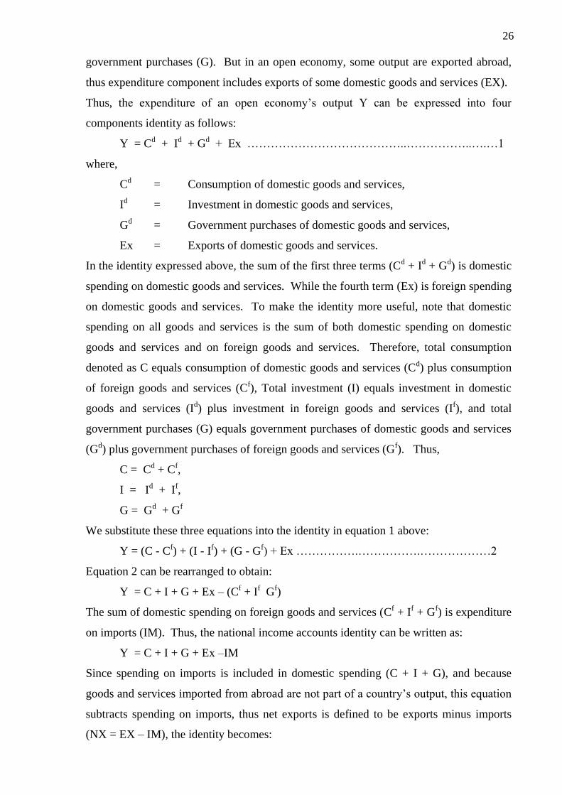
government purchases (G). But in an open economy, some output are exported abroad,
thus expenditure component includes exports of some domestic goods and services (EX).
Thus, the expenditure of an open economy‟s output Y can be expressed into four
components identity as follows:
Y = Cd + Id + Gd + Ex …………………………………..……………..….…1
where,
Cd = Consumption of domestic goods and services,
Id = Investment in domestic goods and services,
Gd = Government purchases of domestic goods and services,
Ex = Exports of domestic goods and services.
In the identity expressed above, the sum of the first three terms (Cd + Id + Gd) is domestic
spending on domestic goods and services. While the fourth term (Ex) is foreign spending
on domestic goods and services. To make the identity more useful, note that domestic
spending on all goods and services is the sum of both domestic spending on domestic
goods and services and on foreign goods and services. Therefore, total consumption
denoted as C equals consumption of domestic goods and services (Cd) plus consumption
of foreign goods and services (Cf), Total investment (I) equals investment in domestic
goods and services (Id) plus investment in foreign goods and services (If), and total
government purchases (G) equals government purchases of domestic goods and services
(Gd) plus government purchases of foreign goods and services (Gf). Thus,
C = Cd + Cf,
I = Id + If,
G = Gd + Gf
We substitute these three equations into the identity in equation 1 above:
Y = (C - Cf) + (I - If) + (G - Gf) + Ex …………….…………….………………2
Equation 2 can be rearranged to obtain:
Y = C + I + G + Ex – (Cf + If Gf)
The sum of domestic spending on foreign goods and services (Cf + If + Gf) is expenditure
on imports (IM). Thus, the national income accounts identity can be written as:
Y = C + I + G + Ex –IM
Since spending on imports is included in domestic spending (C + I + G), and because
goods and services imported from abroad are not part of a country‟s output, this equation
subtracts spending on imports, thus net exports is defined to be exports minus imports
(NX = EX – IM), the identity becomes:
Page 27
27
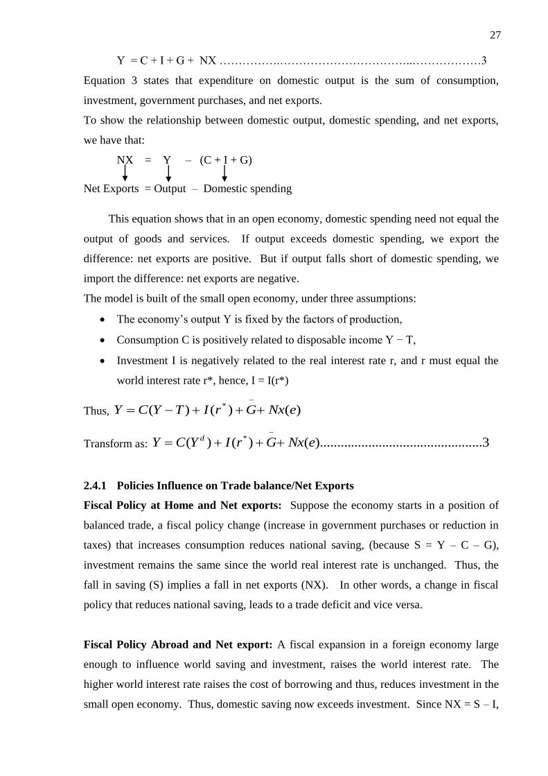
Y = C + I + G + NX …………….……………………………..………………3
Equation 3 states that expenditure on domestic output is the sum of consumption,
investment, government purchases, and net exports.
To show the relationship between domestic output, domestic spending, and net exports,
we have that:
NX = Y – (C + I + G)
Net Exports = Output – Domestic spending
This equation shows that in an open economy, domestic spending need not equal the
output of goods and services. If output exceeds domestic spending, we export the
difference: net exports are positive. But if output falls short of domestic spending, we
import the difference: net exports are negative.
The model is built of the small open economy, under three assumptions:
The economy‟s output Y is fixed by the factors of production,
Consumption C is positively related to disposable income Y − T,
Investment I is negatively related to the real interest rate r, and r must equal the
world interest rate r*, hence, I = I(r*)
Thus, )()()( * eNxGrITYCY
Transform as: 3......................................).........()()( * eNxGrIYCY d
2.4.1 Policies Influence on Trade balance/Net Exports
Fiscal Policy at Home and Net exports: Suppose the economy starts in a position of
balanced trade, a fiscal policy change (increase in government purchases or reduction in
taxes) that increases consumption reduces national saving, (because S = Y – C – G),
investment remains the same since the world real interest rate is unchanged. Thus, the
fall in saving (S) implies a fall in net exports (NX). In other words, a change in fiscal
policy that reduces national saving, leads to a trade deficit and vice versa.
Fiscal Policy Abroad and Net export: A fiscal expansion in a foreign economy large
enough to influence world saving and investment, raises the world interest rate. The
higher world interest rate raises the cost of borrowing and thus, reduces investment in the
small open economy. Thus, domestic saving now exceeds investment. Since NX = S – I,
Page 28
28
the reduction in investment stimulates NX. Hence, fiscal expansion abroad through fiscal
policy leads to a trade surplus at home.
The Real Exchange Rate and Net Exports: Suppose that the real exchange rate is
lower, domestic goods are less expensive relative to foreign goods, domestic residents
purchase few imported goods and foreigners buy many domestic goods. As a result of
both of these actions, the net exports are greater. The opposite occurs if the real exchange
rate is high. The relationship between the real exchange rate and net exports can be
written as:
NX = NX(e)
The equation states that net exports are a function of the real exchange rate.
Trade Policies and Net Exports: Suppose that government through a tariff or quota
prohibits the importation of foreign cars. For any given real exchange rate, imports
would now be lower, thus, this leads to increase in net exports. In other words, a
protectionist trade policy stimulates the trade balance or net exports.
Exchange Rate Fluctuations and Trade flows: The traditional theory is of the opinion
that exchange rate fluctuations depress trade. Fluctuations in exchange rate lead to costs,
risk and uncertainty of profit in international transactions. As a result of this, economic
agents who are only but price-takers in the market; rather than involving in international
transaction with uncertainty of profit in the face of fluctuations would prefer to redirect
their activity from international or foreign trade to home trade and avoid the risk and cost
associated with foreign trade. In other words, exchange rate fluctuations reduce the
volume of international trade.
2.5 LIMITATIONS OF THE PREVIOUS STUDIES
Some previous studies did not take into account the possibility of non-stationarity
in the variables used, yet it is often said that asset prices such as stock prices or
exchange rate follow a random walk. That is, they are non-stationary (Gujarati, 2005).
A time series is said to be stationary if its mean, variance and auto-covariance (at
various lags) remain the same no matter at what point they are measured, (i.e, they are
time invariant) while a non-stationarity time series is a time series with time varying
Page 29
29
mean or time varying variance or both. And for the purpose of forecasting such non-
stationarity time series may be of little practical value.
More also, the model used in the majority of these reviewed studies is based on a
linear regression form:
ttttt VRERYQ 3210
where tQ is the quantity of exports or imports, tY is a measure of economic activity
(GDP or GNP), tRER is the bilateral real exchange rate relevant to the analysis, tV is a
measure of exchange rate fluctuations, and t is a random error term. Hence, in this
model, a statistically significant and negative coefficient for 3 indicates the existence
of a negative relationship between exchange rate fluctuations and trade. While a
statistically significant and positive coefficient for 3 indicates the existence of a
positive relationship between exchange rate fluctuations and trade. These show that
some previous studies neglected to account for the possibility of unit roots, and research
has shown that estimation of regression models of series that have unit roots gives
spurious regression.
Also, some reviewed empirical studies econometrically are incapable of portraying
the dynamic adjustment process to the disequilibrium. Moreover, in their estimations,
the likely long-run linear combination of cointegrating vectors of trade flows and
exchange rate fluctuations, possible effect of macroeconomic policy framework on
exchange rate and also possible transmission effect of exchange rate fluctuations on
exports and imports variability were ignored. Hence, the goal of this study is to address
these neglected issues.
In addition, the current research, apart from introducing dynamism into the study,
will also employ a more popular econometric methodology for a measure of exchange
rate fluctuations, which is GARCH modelling technique, specifically exponential
GARCH (i.e., e-GARCH), which was not used by most previous studies. For instance,
the study by Osuntogun, et al (1993) which indeed, is a pioneering effort to this study
used a measure of exchange rate risk postulated by Caballero and Corbo (1989), which
as pointed out by Pick (1990) is faulty, thus, the estimates of the exchange rate risk
obtained were not standard. That is, according to Pick, such measure over-exaggerates
the risk. However, research has also shown that the analytical framework and the testing
procedure used to measure the influence of exchange rate fluctuations on trade volume
determine the outcome thereof. The choice of exponential GARCH is because it gives a
Page 30
30
scaling property which is in a fairly good agreement with that of real data than its
counterparts and also can easily detect whether the shocks are persistent or not.
2.6 SUMMARY
Attempts have been made to review some related theoretical and empirical
literature to this study. The theoretical background covers what economic theory says
concerning the subject or the a priori information about it, while the empirical literature
discusses the major findings of the existing works, the methods adopted, and their
strengths and weaknesses.
The next section will provide a background to understanding exchange rate
fluctuations in the context of Nigerian economy, its impact on Nigeria‟s trade and
growth, the CBN and other previous policy strategies to deal with the problem, etc.
Page 31
31
CHAPTER THREE
EXCHANGE RATE FLUCTUATIONS IN THE CONTEXT OF NIGERIAN
ECONOMY
3.1 INTRODUCTION
The exchange rate arrangements in Nigeria have undergone significant changes
over the past four decades. It shifted from a fixed regime in the 1960s to a pegged
arrangement between the 1970s and the mid 1980s, and finally, to the various types of
the floating regime since 1986, following the adoption of the Structural Adjustment
Programme (SAP). A regime of managed float, without any strong commitment to
defending any particular parity, has been the predominant characteristic of the floating
regime in Nigeria since 1986 (Sanusi: 2004).
The fixed exchange rate regime induced an overvaluation of the naira and was
supported by exchange control regulations that engendered significant distortions in the
economy. That gave vent to massive importation of finished goods with the adverse
consequences for domestic production, balance of payments position and the nation‟s
external reserves level. Moreover, the period was bedevilled by sharp practices
perpetrated by dealers and end-users of foreign exchange. These and many other
problems informed the adoption of a more flexible exchange rate regime in the context
of the SAP in 1986 (Sanusi: 2004).
3.2 BRIEF OVERVIEW OF EXCHANGE RATE REGIMES
Numerous exchange rate regimes are practiced globally, ranging from the extreme
case of fixed exchange rate system to a freely floating regime. In practice, countries
tend to adopt an amalgam of regimes such as adjustable peg, crawling peg, target
zone/crawling bands, and managed float, whichever suit their peculiar economic
conditions.
a. A Fixed Exchange Rate Regime: It entails the pegging of the exchange rate of the
domestic currency to either unit of gold, a reference currency or a basket of
currencies with the primary objective of ensuring a low rate of inflation. The
advantages and disadvantages of the fixed regime include amongst others, the
reduction of transaction cost in trade, increased macroeconomic discipline,
Page 32
32
possibility of increased credibility due to stability in the exchange rate and
increased response to domestic nominal shocks. A major drawback of the
fixed/pegged regimes, however, is that it implies the loss of monetary policy
discretion (or monetary policy independence).
b. The Floating Exchange Rate Regime: This regime on the other hand, implies that
the forces of demand and supply will determine the exchange rate. The regime
assumes the absence of any visible hand in the foreign exchange market and that
the exchange rate adjusts automatically to clear any deficit or surplus in the market.
Consequently, changes in the demand and supply of foreign exchange can alter
exchange rates but not the country‟s international reserves. Thus, the exchange
rate serves as a “buffer” for external shocks, hence allowing the monetary
authorities full discretion in the conduct of monetary policy. That is, monetary
policy independence, defined in terms of a country‟s ability to control its monetary
aggregates and influence its domestic interest rate and inflation. This is the
greatest advantage of the floating regime. The disadvantages of the freely floating
regime include persistent exchange rate fluctuations, high inflation and transaction
cost.
c. A Variant of the Freely Floating Regime, Managed Floating regime: This
exists when government intervenes in the foreign exchange market in order to
influence the exchange rate, but does not commit itself to maintaining a certain
fixed exchange rate or some narrow limits around it. The bank „gets its hands
dirty‟ by manipulating the market for foreign exchange. Depending on the central
bank‟s intervention, changes in the demand and supply of foreign exchange might
then be associated with changes in the exchange rates and/or changes in
international reserves. Under the system, fiscal and monetary policies are used to
promote internal and external balance (Ekaette, 2002).
Page 33
33
3.3 HISTORICAL AND CURRENT DEVELOPMENTS OF EXCHANGE RATE
POLICIES IN NIGERIA
For an open economy, whose currency is not internationally traded, exchange rate
policy is a key factor in economic management. In other words, the behaviour of an
economy depends on the exchange rate system and policy it has adopted.
Since the establishment of the CBN, Nigeria‟s exchange rate policy, has been
aimed at preserving the external value of the domestic currency and maintaining a
healthy balance of payments position, which indeed, is a major provision of the enabling
law. With the failure of the Autonomous Foreign Exchange Market (AFEM),
introduced in 1995, an Inter-Bank Foreign Exchange Market (IFEM) was introduced in
1999. IFEM was designed as a two-way quote system, and intended to diversify the
supply of foreign exchange in the economy by encouraging the funding of the inter-bank
operations from privately-earned foreign exchange. It also aimed at assisting the naira
to achieve a realistic exchange rate. The operation of the IFEM however, experienced
similar problems and setbacks as the AFEM, owing to supply-side rigidities, the
persistent expansionary fiscal operations of government and the attendant problem of
persistent excess liquidity in the system.
Specifically, the sustained demand pressure and the consequent depreciation of the
naira exchange rate under the IFEM were traced to the following causes:
- Limited sources of foreign exchange supply
- The excess liquidity in the system induced by the transfer of government accounts
from the CBN to banks.
- The huge extra-budgetary spending on unproductive investments.
- The heavy debt service burden; and
- Speculative demand, driven by uncertainties created by social and political unrest,
expectations of future depreciation of the naira as well as the deterioration of the
external sector position.
It became a matter of serious concern that despite, the huge amount of foreign
exchange, which the CBN supplied to the foreign exchange market, the impact was not
reflected in the performance of the real sector of the economy. Arising from Nigeria‟s
high import propensity of finished consumer goods, the foreign exchange earnings from
Page 34
34
oil continued to generate output and employment growth to other countries from which
Nigeria‟s imports originated (CBN: 2003).
This development necessitated a change in policy in 2002, when the demand
pressure in the foreign exchange market intensified and the depletion in external
reserves level persisted. The CBN thus re-introduced the Dutch Auction System (DAS)
to replace the IFEM. The DAS represents an improvement over the previous
mechanisms for determining the exchange rate of the naira, and its operation was/is in
line with the current global trends. However, to further liberalize the foreign exchange
market as a long term strategy in making naira a convertible currency in the future and
also to unify exchange rates such as: inter-bank rates, parallel market rates and official
rates, the CBN established a framework and guidelines for the introduction of a
Wholesale Dutch Auction System (WDAS) after the completion of the recapitalization
and consolidation of the banking industry by the end of 2005. Hence, in 2006 WDAS
was introduced in order to deepen the foreign exchange market and ensure sustained
exchange rate stability (Soludo, 2008).
Furthermore, the strong determination to resolve the fluctuations of foreign
exchange and restore stability made the CBN to suspend the WDAS and in 2008 re-
introduced the Retail Dutch Auction System (RDAS). The RDAS was re-introduced to
check the excesses of market players that engage in speculation, which had slashed the
value of naira against major foreign currencies. Under the RDAS regime, bid for the
purchase of foreign exchange must be cash-backed at the time of the bid and also "funds
purchased from CBN at the auction would be used for eligible transactions only, subject
to stipulated documentation requirements." And such funds "should not be transferable in
the inter-bank foreign exchange market" (Soludo, 2008).
The peculiarity of the Nigerian Foreign Exchange Market needs to be highlighted.
The country‟s foreign exchange earnings are more than 90 per cent dependent on crude
oil export receipts (CBN: 2003). This implies that the fluctuations of the world oil
market prices have a direct impact on the supply of foreign exchange. Moreover, the oil
sector contributes more than 80 percent of government revenue (CBN: 2003).
Therefore, when the world oil price is high, the revenue shared by the three tiers of
government rise correspondingly and, as has been observed since the early 1970s,
elicited comparable expenditure increases, which had been difficult to bring down when
oil prices collapse and revenues fall concomitantly. Indeed, such unsustainable
expenditure level had been at the root of high government deficit spending. It is
Page 35
35
therefore, pertinent that reserves be built up when the oil price is high to cushion the
effect of revenue shortfall on government spending when oil price falls in the
international oil market.
Precisely, throughout the developing world, the choice of exchange rate regime
stands as perhaps the most contentious aspect of macroeconomic policy (Philippe, et al:
2006). Several factors influence the choice of one regime over the other. But the major
consideration is the internal economic conditions or fundamentals, the external
economic environment, and the effect of various random shocks on the domestic
economy. Thus, countries like Nigeria which are vulnerable to unstable internal
financial conditions and external shocks (including terms of trade shocks, and excessive
debt burden), which require real exchange rate depreciation, tend to adopt a regime that
ensures greater flexibility. Generally, there is a consensus that a fixed exchange rate
regime is preferred if the source of macroeconomic instability is predominantly
endogenous. Conversely, a flexible regime is preferred if disturbances are
predominantly exogenous in nature. Nevertheless, it is increasingly recognised that
whatever exchange rate regime a country may adopt, the long term success depends on
its commitment to the maintenance of strong economic fundamentals and a sound
banking system.
Finally, the greatest challenge is to ensure that exchange rate is used as an
appropriate instrument to enhance the productivity of the economy. A strong naira not
supported by the economic fundamentals will only destroy the productive base. But an
appropriate exchange rate will make local production, other things being equal,
competitive. Therefore, to achieve wealth creation and generate employment in the
domestic economy, there is need to change the import dependency syndrome and export
more. Do we want a strong naira? If the answer is yes, our motto should be:
a. To produce more;
b. Import less;
c. Export more; and
d. Buy more Nigerian goods
The right exchange rate, is therefore, the one that facilitates the optimal
performance of the Nigerian economy as a part of the new integrated global village and
make the above objectives (a – d) possible (Sanusi, 2004).
Page 36
36
3.4 GENERAL SURVEY OF NIGERIA’S TRADE POLICIES AND
PERFORMANCE
Trade policy is within the realm of macroeconomic policy. Trade policies broadly
defined, are policies designed to influence directly the amount of goods and services
exported or imported in a country. The Federal Ministry of Commerce is the principal
government agency with the overall responsibility for trade policy formulation,
including for bilateral and multilateral agreements. Under the present political
dispensation in Nigeria, there are three principal organs responsible for decision-making.
These are the Federal Executive Council, the National Council of State and the Senate.
Trade policy ratification ultimately rests with the Federal Executive Council. Until
recently, trade policy formulation and implementation, even though conditioned by the
global context, was dominated by governmental and inter-governmental agencies and
dispersed among several public sector agencies whose responsibilities overlap and
between which coordination is deficient (Afeikhena: 2005).
The major policy thrusts of the Nigerian trade policy includes integrating the
economy into the global market system, liberalization to enhance competitiveness of
domestic industries, effective participation in trade negotiations to harness the benefits
in the multilateral trading system, adoption of appropriate technologies and support of
regional integration and corporation. The export policy seeks to diversify the export base
of the economy and replace the mono-commodity export orientation configured by the
dominant petroleum exports. The import policy is concerned with further liberalization
of the import regime to promote efficiency and international competitiveness of
domestic producers. In reviewing trade policies of the past, the government‟s policy
framework acknowledges that:
… trade and distribution were characterised by inter-regional trade barriers, many
layers of distribution that raise the cost of goods; bureaucracy in the
implementation of trade incentives including long delays in business registration,
payment of export-rebate incentives etc; and the dumping of substandard and
subsidised goods. The non implementation of the ECOWAS Treaty on Free Trade
for many years after its ratification served as a serious disincentive to exploring
the potential of West Africa Trade. The large number of security agents at the ports
and the long procedures for goods clearance were further impediments to trade.
Page 37
37
3.5 TRADE AND THE NIGERIAN ECONOMY
Nigeria is still predominantly a mono-cultural economy. It depends heavily on the
oil sector. Hence, the country is exposed to shocks beyond the control of the
government. The economy still has lingering problems of low output growth relative to
the population growth rate, unemployment and poor infrastructural amenities. Economic
recovery or slowdown still largely depends on crude oil sales. In fact, the pace of
economic recovery suffered a setback following intensification of pressure on external
sector as the world price of oil slumped in the late 1990s while the growth rate of non-
oil exports remained weak. However, the pressure on the balance of payments eased
considerably in 2000, because of the effect of higher oil prices in the international
market. These instances expose the economy‟s unsustainable degree of dependence on
the oil sector.
Table 1: Value of Nigeria’s exports and imports, 1996 – 2004
Year Exports of Goods (US $ million) Imports of Goods (US $ million)
1996 16,117 6,438
1997 15,539 9,630
1998 10,114 9,276
1999 11,927 10,531
2000 20,441 12,372
2001 17,261 11,585
2002 15,107 7,547
2003 19,887 10,853
2004 31,148 14,164
Source: Central Bank Annual Reports, Various Issues
The table above shows that the value of exports declined between 1997 and 1999,
but rose again in 2000. This is mainly due to the drop in oil prices during the period. The
table also shows an increase in imports, which was the result of increased demand for
finished goods and foreign inputs for the manufacturing sector during the period. In
general, the fluctuations in total exports and imports are usually attributable to
fluctuations in the sales of crude oil.
The direction of Nigeria‟s trade is also indicative of the structure of trade in the
country. A simplified version of Nigeria‟s trade directions is presented below. From the
table, the flow of exports shows the dominance of intercontinental trade while intra-
Page 38
38
Africa trade is very minimal, albeit the slight increase over the period. With reference to
exports, the table shows that United States remained the largest buyer of Nigeria‟s
exports (UNCTAD: 2001). Thus, in view of the excessive dependence of Nigeria‟s
trade on sales to the USA, it is imperative that regional trade particularly, within the
West African sub-region, be boosted as part of the drive towards establishing a private-
sector driven economy.
Table 2: Main Origins of Nigeria’s Exports and Imports (% of total)
Exports Imports
USA 46.1 UK 10.9
Spain 10.7 USA 9.2
India 6.1 France 8.7
France 5.2 Germany 7.4
Source: UNCTAD 2001
3.6 THE IMPACT OF EXCHANGE RATE FLUCTUATIONS ON NIGERIA’S
TRADE AND GROWTH
The evil effect of having an over-valued exchange rate is legion. The most critical
is the creation of a high propensity to import because an over-valued currency makes
import cheaper and promotes balance of payments deficits. Nigeria experienced an
unsustainable demand for foreign exchange in the early 1980s when the government
resorted to exchange control mechanism to support the over-valued naira. Also, the days
of foreign exchange rationing through import licensing created suffocating distortion
and corruption, to the Nigerian economy. The economic agents have resources in naira
that command more foreign exchange at the official rate than could be made available,
hence, foreign obligations contracted, which could not be settled immediately
subsequently, crystallised into Paris and London Clubs foreign debts. These debts, with
the accrued interest and penalties, constituted more than 80 per cent of Nigerian total
external debt. Indeed, most of these debts were not incurred by the government but
rather by Nigerian private sector induced by over-valued naira.
Furthermore, the period when exchange rate was $1.8 to the naira did incalculable
damage to the economy. It destroyed the agricultural base as food import became so
cheap that farmers abandoned their farms and became traders. The manufacturing sector
was not spared. A new culture of import dependency was created, which proved slow
Page 39
39
and difficult to change and at a painful cost caused frustrations and discomfort in the
land. Hence, the most critical factor and challenge, however, remains how to increase
the productivity of the domestic economy. The higher the productivity, the lesser the
pressure on the naira exchange rate and its fluctuations, and all the structural rigidities
facing the economy would be reduced to the barest minimum if they cannot be
completely eliminated.
In general it is imperative to let the exchange rate find its equilibrium level, as it is
only when the equilibrium exchange rate prevails that there is viability of the balance of
payments position. Moreover, a stable foreign exchange rate regime will lead to
macroeconomic stability and encourage investment and growth, reduce capital flight and
encourage capital inflows in the form of foreign private investment.
3.7 THE CBN’S POLICY RESPONSES TO EXCHANGE RATE
FLUCTUATIONS
The need to ensure that a realistic exchange rate of the naira is achieved has been a
major objective of the Central Bank of Nigeria. This is because a realistic exchange rate
would result in the simultaneous achievement of sustainable economic growth and
development. Indeed, the CBN has gone a long way in evolving an enduring exchange
rate management policy, and have no doubt made appreciable progress in this regard. A
realistic exchange rate would ensure that the naira is not overvalued in real terms, and
that the external sector remains competitive.
However, in the quest for a realistic naira exchange rate, the CBN employs the
Purchasing Power Parity (PPP) model as a guide to gauge movements in the nominal
exchange rate and to determine deviations from the equilibrium exchange rate. Although
the PPP as a relative price does not provide clear criteria for choosing a base period, and
is generally criticized for its insensitivity to short-term policy actions, it nonetheless,
provides a reasonable framework for a comparative analysis of trading partners‟
performances (Sanusi, 2002).
The monetary authority also usually intervenes through its monetary policy actions
and operations in the money market to influence the exchange rate movement in the
desired direction such that it ensures the competitiveness of the domestic economy. For
instance, in 2002, the CBN adopted a medium term monetary policy framework subject
to periodic amendments in order to free monetary policy implementation from the
problem of time inconsistency and minimize over-reaction due to temporary shocks.
Page 40
40
Also, in 2005, some new reforms were introduced as “amendments and addendum”
to the monetary policy circular, which include: exchange rate band (of +/- 3.0%), in
which under the West African Monetary Zone Exchange Rate Mechanism (ERM)
arrangement, member countries are required to maintain a band of +/- 10.0%. The band
was intended to anchor expectations, enable investors and end-users of foreign exchange
to plan and minimize transaction costs and also discourage the destabilising practices of
speculation and hoarding. However, the CBN maintained a narrower band of +/- 3.0%
due to the appreciable level of external reserves and the relative stability of naira
exchange rate achieved then (Soludo, 2008).
In Nigeria, maintaining a realistic exchange rate for the naira is very crucial, given
the structure of the economy, and the need to minimize distortions in production and
consumption, increase the inflow of non-oil export receipts and attract foreign direct
investment. Moreover, the persisting problems of import dependency, capital flight, and
lack of motivation for backward linkages in the production process need to be addressed,
amongst others.
And to this end, the CBN is ready to consider suggestions on possible strategies for
enhancing the efficiency of foreign exchange management in Nigeria, particularly in
meeting the urgent need, which is to strengthen and diversify the non-oil export base of
the economy.
3.7.1 Other Policy Strategies to tackle Exchange Rate Fluctuations
The government has committed itself to strengthening trade as an instrument for
achieving accelerated economic development. Some of the government‟s strategies as
documented in her policy direction for foreign trade include:
Effective implementation of incentives and their review;
Establishment of market search of exports houses;
Bilateral trade negotiations to diversify trade;
Establishment of reciprocal trade and investment centres;
Establishment of a databank on trade and related matters;
Adoption of measures for exploring Africa‟s potential for trade;
Continuous reforms at ports, and measures to check dumping;
Effective implementation of the ECOWAS Protocol on free movement of goods and
people;
Page 41
41
Full operationalisation of the existing Export Promotion Zones (EPZs), the
establishment of new ones, and the granting of export-processing status to deserving
factories that contribute to non-oil exports; and
Institutional strengthening and reorientation of staff, and streamlining of procedures
and processes (Akindele: 1988, Isitua, et al: 2006)
The implementation of some of these policies is underway in Nigeria. These
include review of customs tariffs with a view to raising revenue, as well as protecting
domestic industry, import-prohibition strategies, aimed at not only boosting
government‟s revenue base, but encouraging the agricultural sector, thereby increasing
the income of farmers. Export promotion and incentives to encourage non-oil exports
and reduce the over-dependence on oil revenue are also being encouraged. Other
measures being implemented are the liberalization of trade in accordance with the
demands of international financial institutions and the ECOWAS Trade Liberalization
Scheme (TLS), and inspection at destinations to replace pre-shipment inspection.
Page 42
42
CHAPTER FOUR
RESEARCH METHODOLOGY
This chapter discusses the analytical framework of the models used, data
transformation, model specification and justification, sources of data, and finally,
estimation technique and procedure used for the research work.
4.1 ANALYTICAL FRAMEWORK OF THE MODELS USED
To provide a deep insight into the relationship between exchange rate fluctuations
and trade flows; we assess the effect of different macroeconomic policies on exchange
rate in Nigeria with emphasis on Mundell Fleming Model. In other words, find out if
the fluctuations of exchange rate are as a result of poor implementation of policies or
that the policy framework is not favourable in the context of the adopting country
(Nigeria). This is because it is possible that the hesitant conclusions reached by
previous studies may have been partly attributed to their failure to consider first the
effect of different policy frameworks on exchange rate.
Also, the study adopts a standard econometric methodology for a measure of
fluctuations which is GARCH modelling technique, which was not used by most
previous studies. In addition, there is much evidence that a lagged relationship may
exist between the volume of trade and its determinant (exchange rate fluctuations);
hence, this study explicitly takes this possibility into account by adopting a VAR model,
which allows for joint estimation of relationships between trade and exchange rate
fluctuations, as well as how past information relate to the perceived fluctuations. Other
standard trade models tend to ignore the possibility of such a lagged relationship.
More also, a multivariate Johansen cointegration test is adopted to assess the long
run linear combination of the cointegrating vectors of exchange rate fluctuations and
trade flows and with evidence of cointegration, the VAR model is then reformulated into
a vector error correction model to know whether the disequilibrium in trade could be
corrected back to its equilibrium position. (That is, the short run dynamic adjustment
process by which trade could converge on its equilibrium long run value). Thus, the
model makes a clear distinction between the long-run and the short-run effects.
Finally, we equally ascertain the transmission level of exchange rate fluctuations
on exports and imports (trade) variability in Nigeria and the dynamic effect of shocks on
Page 43
43
the endogenous variables using both the impulse response and variance decomposition
analyses.
4.2 DATA TRANSFORMATION
Considering the following model:
1..................................................................43210 tttFtDtt WExYYX
where,
Xt = Trade flows (Oil & Non-oil exports plus imports) at time t
YDt = Domestic income at time t
YFt = Foreign income at time t
Ext = Bilateral exchange rate at time t
Wt = Exchange rate fluctuations at time t
Therefore, since equation 1 holds true at every time period, it equally holds in the
previous periods in the past, (t – 1), (t – 2), etc. Thus, equation 1 can be written as:
2....................................................43210 itititiFtiDtit WExYYX
where,
itX , iDtY , iFtY , itEx , itW and it represent unknown values of X, YD, YF, Ex,
W and respectively to be estimated.
Subtracting equation 2 from equation 1, we obtain
3.............................................................4321 tttFtDtt WExYYX
where,
= First-difference operator (telling us to take successive differences of the variables
in question. Thus, 1 ttt XXX , 1 DtDtDt YYY , 1 FtFtFt YYY , 1 ttt ExExEx ,
and 1 ttt .
To express the coefficients in elasticity form and also reduce the standard errors of the
variables, we can transform equation 3 into:
4............................................4321 tttFtDtt InWInExInYInYInX
where, 1 tttt
Page 44
44
1......................................................................................................'
0 ttt YX
iidt ~ 2...............................................................................................).........,0( 2
tN
Thus, equation 2 is known as the level form while equation 3 is known as the first
difference form. Both forms are often used in empirical analysis. But instead of
studying the relationships between the variables in the level form, we are interested in
their relationships in the growth form, which is the first-difference form. Thus, in
equation 4, InX , DInY , FInY , InEx and InW represent changes in the logs of
trade flows, domestic and foreign income, bilateral exchange rate and fluctuations
respectively, where a change in the variable is a relative or percentage change (if
multiplied by 100).
The model in equation 4 is known as dynamic regression model (that is, model
involving lagged regressand). To justify for the assumption of no autocorrelation in
equation 4, Durbin-Watson (D-W) d test is used. The first-difference transformation is
said to be appropriate if the D-W d is quite low. In the words of Maddala, use the first-
difference form whenever d < R2. While the choice of optimal lag length for the VAR
specification is determined using both the Akaike (AIC) and Schwarz (SC) information
criteria.
4.3 MODEL SPECIFICATION
We obtain the conditional fluctuations values from the estimated variance equation
of the GARCH model developed by Bollerslev (1986) and advanced by Nelson (1991).
We therefore specify the following GARCH (p, q) model:
In the above mean equation, Xt = Individual time series data of the variables of
interest while Yt is a (k x 1) vector of explanatory variables and it includes also
autoregressive terms of the dependent variables.
The initial condition is assumed to be:
Thus,
3...........................................................................11
2
1
2
0
2
n
k
kk
q
jjt
j
p
iitit
Y
Equation 3 is the variance equation, which states that the value of the variance scaling
parameter 2
t depends on both its past values captured by lagged 2
t terms and on the
Page 45
45
lagged squared residuals terms. While Yk is a set of explanatory variables that might
help to explain the variance equation.
To guarantee that the forecasts/estimates of the conditional variance are
nonnegative, we modify the variance equation in equation 3 by adopting the exponential
GARCH developed by Nelson (1991). He propounded E-GARCH to solve the
restriction problem of GARCH models (that is, problem of persistence of shocks to
conditional variance).
Thus, the generalized E-GARCH (p, q) model for the conditional variance is:
4.....................111
22
q
j jt
jt
j
jt
jt
j
n
k
kk
p
iitit
YInIn
where,
jki ,,, and j are parameters to be estimated. Therefore, the left hand side being
In of the conditional variance, implies that the leverage effect is exponential not
quadratic, hence, the estimates of the conditional variance are positive.
4.3.1 Introductory Explanation of the Net Export Equation
To attempt to predict the effects of major policy changes by using econometric
models of the economy based on data recorded when different policies were in place is
dangerous (Black, 2003). Individuals, firms and policy makers rather are assumed to
choose their actions in the light of existing policies; for example, choice of the variables
in the net exports equation takes account of different policy frameworks affecting
exchange rate in Nigeria. Hence, if there is a major policy change, this changes the
incentives in the system and will change economy‟s conduct. It cannot be assumed that
the effects of a major policy change can be predicted just by changing particular
parameters in a few fitted equations. The general implication of this critique is that the
effects of policy framework changes are hard to forecast (Lucas effect); they can be
learned by experience.
Therefore, in this study, the effect of different macroeconomic policy frameworks
on exchange rate in Nigeria can be learned from their effects on the net exports equation
specified.
Although the selection of the correct total trade equation in general and that of an
export equation in particular is problematic, we adapt the specification by Taglioni
Page 46
46
(2002) who analyze the relationship between exchange rate volatility and trade flows for
East and Central European countries in a very meticulous and systematic way.
The net exports equation is estimated in nominal terms thus, the implicit function of this
model takes the form:
aImpfNx VF 5..............................................................Ex).......,,Y,(YD
While the model for the net exports equation for objective one is specified as:
bExImpYYNx ttVFDot ttt5................................4321
where,
Nxt = Net Export value at time t
YDt = Domestic income at time t
YFt = Foreign income at time t (the USA income)
ImpVt = Import tariff at time t (proxy as value of imports at time t)
Ext = Bilateral exchange rate at time t
Also the total trade equation for the VAR model to capture the other objectives can be
written as:
6..................................43210 tttFttDt WExYYX
(Note, the variables are as explained before in equation 1 of data transformation).
Economic theory suggests that the impact of nominal or real domestic and foreign
income and also that of import tariff (proxy by import values) on net exports and trade
should be positive. While a fall in exchange rate (rise) may leads to an increase
(decrease) in net exports due to the relative price effect. Finally, the effect of exchange
rate fluctuations on trade flows is yet inconclusive. However, according to Taglioni
(2002), which we adapt, it is negative. In other words, it is expected that 1 / 1 , 2 / 2 ,
and 3 > 0 while, 4 / 3 , and 4 < 0.
We shall estimate the reduced form n-variable VAR model of order k as follows:
7.........................................................................................................1
0 t
n
iitit ZZ
where,
Z = vector of endogenous variables
Page 47
47
i = parameters ( ,,, and ) to be estimated
The impulse responses and variance decompositions computed from the VAR
estimates are used to ascertain the reaction of trade flows to exchange rate fluctuations
and the dynamic effect of shocks on the endogenous variables included in the model.
The further analysis to variance decomposition is needed as it offers information on the
relative importance or predictive content of each of the determinant variables regarding
the dependent variable.
We also specify the VAR model in equation 7 as follows:
The level of variations in trade flows from each of the endogenous regressors
determines how significant or not, shocks from such variable are to the Nigerian trade
flows. For instance, if shock from the exchange rate fluctuations is high, it implies that
exchange rate fluctuations are important determinant of variations in exports and imports
in Nigeria.
To asses the long-run linear combination of the cointegrating vectors of trade flows
and exchange rate fluctuations, the Engle Granger two-step approach to Error Correction
Model (ECM) and the multivariate Johansen procedure are adopted. However, the
Vector Error Correction Model (VECM) is a convenient model setup for cointegration
analysis. Therefore, the VAR model above is reformulated into a vector error correction
model with the evidence of co-integration as follows:
aZZZZZ ttktkttt 8................................... 1112211
aWExYYXX t
n
i
iti
n
i
iti
n
i
Fi
n
i
Diit
n
i
it itit7..1
11111
0
bXWExYYY tit
n
i
i
n
i
iti
n
i
iti
n
i
Fi
n
i
DitD itit7..2
11111
0
cYXWExYY t
n
i
Diit
n
i
i
n
i
iti
n
i
iti
n
i
FiFt itit7..3
11111
0
dYYXWExEx t
n
i
Fi
n
i
Diit
n
i
i
n
i
iti
n
i
itit itit7..4
11111
0
eExYYXWW t
n
i
iti
n
i
Fi
n
i
Diit
n
i
i
n
i
itit itit7...5
11111
0
Page 48
48
The reduced form p-variable dynamic VECM representation as:
bZZZ tt
p
i
itit 8............................................................................1
1
1
where,
Z = a vector of endogenous variables
Note, since tZ does not contain I(1), hence must be I(0), the term 1tZ is the only
one that includes I(1) variables, thus contains the cointegrating relations.
i = short-run parameters
1tZ = long-run part, that is, the matrix contains information regarding the long-run
relationships.
Suppose that r)(rank
Then we can decompose the matrix = '
rrkrxn )( ) (
rrkrk )( )(
where, includes the speed of adjustment to equilibrium coefficient while '
represents long run matrix of coefficients of cointegrating relation. After testing for the
existence of cointegration, it is useful to reparameterize the model in the equivalent
ECM form (Johansen, 1988) as follows:
9.....5
1
4
1
3
1
2
1
10 titlt
p
l
lkt
o
k
kF
n
j
jD
m
i
it ecmWExYYXjtit
where,
itlkFtjDtiit ExYYecm
t4t3210t ΔWλΔλΔλΔλλΔX , is the residual of the
cointegration equation and it estimates the speed of convergence of the dependent
variable back to equilibrium after changes in the other variables.
5λ = Adjustment parameter shows how the disequilibrium in the dependent variable is
being corrected each period. If statistically significant, it implies the
disequilibrium will be corrected at different period, otherwise, at the same period.
n
i 1
= Summation of the range of the variables
= Difference operator
rrkrxn )( ) (
Page 49
49
4.4 JUSTIFICATION OF THE MODELS USED
Multiple regression analysis and vector autoregressive (VAR) model are the
statistical framework for the research study. The choice of VAR model is based on the
fact that it allows for joint estimation of relationships between exchange rate fluctuations
and trade flows, as well as how past information relate to perceived fluctuations. Also,
it assumes that the information relevant to the prediction of the respective variables is
contained solely in the time series data of these variables and the disturbances
uncorrected. More also, variance decomposition as an aspect of VAR is one of the most
popular techniques for capturing the impulse responses and transmission of shocks
among the variables.
Furthermore, the GARCH model is considered suitable to measure fluctuations
because it provides a rich class of possible parameterizations of heteroskedasticity. Also,
GARCH model is more parsimonious, and avoids over-fitting. According to Qian and
Varangis (1992), the advantages of this approach over other approaches are, first, the
risk from exchange rate fluctuations is explicitly modelled and included as a regressor in
the trade volume equation, thus, avoiding arbitrariness in defining the measure of
fluctuation risk. Second, possible heteroskedasticity will be taken into full account in
the estimation process, hence avoiding the possibility of biased estimates of the test
statistic. The estimation of fluctuations or volatility using the GARCH modelling
technique as used by Kroner and Lastrapes (1991) follows the process: First, we obtain
the residual from the AR equation of the real exchange rate. Second, obtain squared
residuals from the equation and finally, estimate the AR equation of the squared
residuals to get a measure of fluctuations (Gujarati, 2005).
Trade flows are taken to cover both the oil and non-oil exports and imports.
Economic theory suggests that domestic income, denoted as YD and income in an
importing country denoted as YF, and also exchange rate between a country and its
major trading partner (e.g., US), denoted as Ex are important determinants of a country‟s
trade. In other words, they are conventionally treated as determinants of exports and
imports supply, while the exchange rate fluctuations is estimated and incorporated into
the equation as one of the explanatory variables.
4.5 SOURCES OF DATA AND VARIABLES USED
The dependent variable in the study is the Nigeria‟s trade flows (both oil and non-
oil) to the United States for the period between 1980 and 2008, and is denoted as X. The
Page 50
50
secondary data for the variables used are extracted from the CBN Statistical Bulletin
(various issues) and National Bureau of Statistics.
4.6 ESTIMATION TECHNIQUE AND PROCEDURE
We adopt method of maximum likelihood in our estimations. Evaluations of
results are based on three criteria, namely, economic criterion – a priori behaviour of the
parameters and their economic implications, statistical criterion – use of R2, F, and t-
statistics to test the explanatory power of the estimated parameters, and finally,
econometric criterion – reliability of the estimated parameters – consistency and
sustainability of the explanatory power of the parameters. While econometric views (E-
views) version 5.0 is the software package used for the estimations.
4.6.1 Procedure
The estimation commences with an extensive unit root test to confirm the
stationarity states of the variables that entered the model using both the Augmented
Dickey-Fuller (ADF) and Phillips-Perron (PP) tests. Both tests of unit root are used in
order to guarantee that our inferences regarding the important issue of stationarity are
not likely driven by the choice of the testing procedure used.
The testing procedure for the ADF test is as follows:
tptpttt XXXtX ...1110
where, 0 is a constant, t is the coefficient on a time trend and p is the lag order of the
autoregressive process and is the difference operator. The unit root test is then carried
out under the null hypothesis = 0 against the alternative hypothesis of < 0. We
compare the computed value of the test statistic with the relevant critical value for the
test. For instance, if the computed test statistic is greater (in absolute value) than the
critical value at 5% or 1% level of significance, then the null hypothesis of = 0 is
rejected and thus no unit root is present, otherwise, it is accepted.
The test for stationarity is first conducted at level, however, if the variables are not
stationary at level; we then difference them and test for the stationarity of the
differenced variables. Supposing the variables are stationary at first difference, we
conclude the variables are integrated of order one (i.e., I(1)).
Page 51
51
4.6.2 Cointegration Tests
Having confirmed the stationarity properties of the variables, we proceed to
determine the existence of a long-run relationship among these variables. A co-
integrating relationship exists between series, if there is a stationary linear combination
between them. To ensure a robustness check of the cointegration estimation, we used
both the Engle-Granger approach and the Johansen maximum likelihood procedure.
Using the Engle-Granger procedure of cointegration test, we first regress the dependent
variable on its various determinants to obtain the estimated coefficients, then estimate
the residuals from this regression and save it and finally, test if the saved estimated
residual series is stationary or not. However, since the Engle-Granger approach suffers
problem of normalization, the multivariate Johansen procedure, which uses maximum-
likelihood method of estimation and does not suffer normalization problem (Gujarati,
2005) is fully utilized.
A multivariate Johansen cointegration test is adopted to assess the long-run linear
combination of the cointegrating vectors of exchange rate fluctuations and trade flows
and if there is evidence of cointegration, the VAR model is reformulated into a vector
error correction model (VECM) to know whether the disequilibrium in trade could be
corrected back to its equilibrium position.
Finally, the analyses are complemented with impulse response and variance
decomposition mechanisms to ascertain the transmission level of exchange rate
fluctuations on trade variability and the dynamic effect of shocks on the endogenous
variables included in the model.
Page 52
52
CHAPTER FIVE
DATA PRESENTATION AND DISCUSSION OF RESULTS
5.1 INTERPOLATION OF TIME SERIES DATA
To ensure adequate observations for the time series analysis, the interpolation
approach which strongly utilizes the properties inherent in the actual quarterly series was
used to decompose the annual series to quarterly using the process or formular below:
0.75A1 + 0.25A2 .. .. .. .. 1st quarter
0.5A1 + 0.5A2 .. .. .. .. 2nd quarter
0.25A1 + 0.75A2 .. .. .. .. 3rd quarter
A1 .. .. .. .. 4th quarter
Table 3: Example of Interpolation of Data
1 Year Quarter
Annual Data
(Assumed as Column B)
Formular for
Interpolation
Result of Interpolated
Data
2 1980 Q1 0.5464 0.75B2 + 0.25B3 0.5623
3 Q2 0.61 0.5B2 + 0.5B3 0.5782
4 Q3 0.25B2 + 0.75B3 0.5941
5 Q4 B2 0.5464
6 1981 Q1 0.61 0.75B6 + 0.25B7 0.625725
7 Q2 0.6729 0.5B6 + 0.5B7 0.64145
8 Q3 0.25B6 + 0.75B7 0.657175
9 Q4 B6 0.61
Note: In interpolation using Excel, the 1st row must be used for labels, and the 1
st observation must begin
from the 2nd
row while the 1st column must be for year. Then after interpolating the 1
st observation (e.g.,
1980), highlight the interpolated data for that 1st observation (i.e., 1980) and apply auto fill to interpolate
the other series.
5.2 TIME SERIES PROPERTIES
We determine the stationarity properties of the variables using two tests of unit
roots, namely the Augmented Dickey-Fuller (ADF) and the Phillips-Perron Tests. While
the ADF procedure is perhaps the most commonly used test, it nevertheless requires
homoscedastic and uncorrelated errors in the underlying structure. The PP non-parametric
test generalizes the ADF procedure, allowing for less restrictive assumptions for the time
series in question. We used both tests of unit root in order to guarantee that our inferences
Page 53
53
regarding the important issue of stationarity are not likely driven by the choice of the
testing procedure used. The results of the tests are presented in table 4. The results from
both tests show that none of the series is stationary at level as their test statistic are all
smaller than the 5% critical value of -2.887 for rejection of hypothesis of a unit root.
However, the null hypothesis of non-stationarity is consistently rejected for all the
variables when they are expressed in first differences, suggesting that they are all
integrated of order one (I(1)). The results reported are for those with intercept. However,
the results with trend and intercept were not significantly different. See appendix 1 for
the detailed results of ADF test.
Table 4: Unit Root Test Results
ADF TEST PHILLIPS-PERRON TEST
Variable
Level
1st Difference
Level
1st Difference
Order of
Integration
X
Nx
YD
YF
ImpV
Ex
0.114318
-1.084100
2.190537
-1.351308
0.247726
-0.978992
-8.656687*
-19.69537*
-9.012390*
-11.12520*
-8.455986*
-13.29683*
0.817321
1.588428
1.908211
-1.004622
0.728731
-0.897728
-9.216683*
-18.69526*
-9.198508*
-6.949987*
-10.06517*
-12.41982*
I (1)
I(1)
I (1)
I (1)
I (1)
I(1)
Note: * denotes the rejection of null hypothesis of a unit root for both tests. The lag order
for the series was determined by the AIC and SIC.
5.2.1 Influence of Policies on the Trade balance/Net Exports
Having understood the links among the key macroeconomic variables that
measure interactions in an open economy with Mundell-Fleming model, we employ the
model to answer how the trade balance responds to changes in policy (i.e., the effect of
different policy changes (fiscal, monetary and trade policies) on net exports). The result
is presented in table 5.
Page 54
54
Table 5: Effect of Different Macroeconomic Policies on Net Exports/Trade
Balance
Dependent Variable: NX
Method: Least Squares
Sample: 1980Q1 2008Q4
Included observations: 116
Variable Coefficient Std. Error t-Statistic Prob.
C -900922.10 277591.30 -3.25 0.00
YD 0.49 0.13 3.92 0.00
YF 187.48 57.78 3.25 0.00
IMPv 0.11 0.20 0.55 0.58
EX -6791.318 2521.713 -2.693137 0.01
R2 = 0.80
Durbin-Watson stat = 1.23 Prob(F-statistic) = 0.00
ExImpYYExportsNet VFD 3180.67911088.04814.1874897.013.900922
The estimated result shows that all the variables except import tariff proxy by
import value are statistically significant and with correct signs. The estimated coefficient
of domestic income as 0.49 implies that for any 1 unit increase in domestic income, net
exports increases by about 49%. The result tends to support the economic theory of a
positive relationship between domestic income and net exports. The coefficient of
foreign (US) income as 187.48 supports the other findings below that increase in US
income exerts high effect on net exports. However, 1 unit increase in US income has a
positive influence of about 187.5% on trade balance. Indeed, this effect is highly
significant.
Furthermore, the coefficient of import values as 0.11, which is indicator for import
tariff, implies that for any 1 unit increase in import tariff, net exports increases
approximately by 11%. However, this increase in net exports as a result of the
protectionist trade policy (import tariff) is not statistically significant. This surprising
conclusion is often overlooked in the popular debate over trade policies. Because a trade
deficit reflects an excess of imports over exports, one might guess that reducing imports
such as by prohibiting or imposing duties on the import of foreign goods would reduce a
trade deficit. Yet our estimated model shows that protectionist policies can lead only to
an appreciation of the real exchange rate. And the increase in the price of domestic goods
Page 55
55
relative to foreign goods tends to lower net exports by stimulating imports and depressing
exports. Thus, the appreciation offsets the increase in net exports that is directly
attributable to the trade restriction. Although trade policies do not alter the trade balance,
they do affect the amount of trade. This fall in the total amount of trade is the reason
economists almost always oppose protectionist policies. Protectionist trade policies
diminish the gains from international trade. Although these policies benefit certain
groups within the society, for example, a ban on imported cars helps domestic car
producers but the society on the average is worse off when policies reduce the amount of
international trade. The analysis above shows that protectionist trade policies do not
affect significantly the trade balance.
Finally, the result of exchange rate is statistically significant at 5% level of
significance and with correct sign of negative. This tends to corroborate the theory,
which states that a high (low) exchange rate leads to reduction (increase) in net exports.
The overall conclusion drawn from the estimated result above is that for improved
balance of trade in Nigeria, coordination between the exchange rate and demand
management policies should be strengthened and be based on the long-run fundamentals
of the economy. However, one cannot judge economic performance from the trade
balance alone. Instead, we must look at the underlying determinants of the international
flows. In other words, we carry out further analysis of the impact of the various proposed
determinants of trade flows on trade.
5.3 COINTEGRATION ANALYSES
Having confirmed the stationarity properties of the variables and assessed the
influence of policies on net exports, we proceed to determine the existence of a long-run
relationship among these variables. But before this, we consider the optimal lag length for
the VAR specification. The results of two different information criteria, Akaike (AIC)
and Schwarz (SC) used unambiguously show that the optimal lag length is two. To do a
robustness check of the cointegration estimation, we used both the Engle-Granger
approach and the Johansen procedure.
Table 6 presents the results of cointegration tests using the Engle-Granger procedure for
trade flows. First, we regress Zt on Xt, and obtain the estimated coefficients, estimate the
residuals from this regression and save it and test if the residual series is stationary.
Page 56
56
Table 6: The Engle-Granger Cointegration Tests
Zt Xt t-Statistic Prob.
Trade
Trade
Trade
Trade
Domestic Income (YD)
Foreign Income (YF)
Bilateral Exchange rate (Ex)
Exchange rate fluctuations (W)
-9.82
-16.99
-9.77
-9.79
0.00
0.00
0.00
0.00
From the Engle-Granger procedure, it appears that all the variables are cointegrated
with trade. However, according to Banerjee, et al (1986), substantial bias occurs in the
estimation method of Engle-Granger procedure, which is based on OLS method.
Therefore, we also applied Johansen method, which uses maximum-likelihood method of
estimation to ascertain the number, if any, of cointegrating relationships in the vector
autoregressive equation. The results of the Johansen cointegration test are presented in
table 7, and both the Maximum Eigen-value and the Trace Statistic are reported.
Table 7: Multivariate Johansen Cointegration Test Results
Cointegration Vector (series) = (X, W, YD, YF, Ex)
Null
Hypothesis
Alternative
Hypothesis
Eigen Value Trace
Statistic
0.05
Critical Value
Probability
r = 0
r ≤ 1
r ≤ 2
r ≤ 3
r ≤ 4
r = 1
r = 2
r = 3
r = 4
r = 5
0.604150
0.326748
0.132621
0.056902
0.013637
172.1382
68.34568
24.03458
8.099340
1.537847
69.81889
47.85613
29.79707
15.49471
3.841466
0.0000
0.0002
0.1990
0.4549
0.2149
Null
Hypothesis
Alternative
Hypothesis
Eigen Value Max-Eigen
Statistic
0.05
Critical Value
Probability
r = 0
r ≤ 1
r ≤ 2
r ≤ 3
r ≤ 4
r = 1
r = 2
r = 3
r = 4
r = 5
0.604150
0.326748
0.132621
0.056902
0.013637
103.7925
44.31110
15.93524
6.561493
1.53847
33.87687
27.58434
21.13162
14.26460
3.841466
0.0000
0.0002
0.2287
0.5423
0.2149
For both the maximum eigen value and trace statistic, the null hypothesis is that
there are r cointegrating vectors while the alternative hypotheses are r+1 and at least r+1
Page 57
57
cointegrating vectors for the maximum eigen-value and trace statistic, respectively.
Overall, from the Johansen cointegration test results in table 4, both the trace and the
max-eigen value tests indicate that there are two cointegrating equations among the
variables at 5% level of significance.
Therefore, we get different findings following the Engle–Granger procedure and the
multivariate Johansen method. But we assigned more importance to the results obtained
by Johansen, which uses maximum-likelihood method of estimation than the ones from
the Engle–Granger procedure, because the former has significant power advantage over
the latter. Cheung and Lai (1993) show that the Engle–Granger procedure has very low
power in rejecting the no cointegration hypothesis even when an equilibrium relationship
in fact holds in the long run. Another limitation of the Engle–Granger procedure is that it
does not account for the possibility of multiple cointegrating relationships.
Furthermore, Phillips (1991), shows that the maximum-likelihood coefficient
estimator is super-consistent, symmetrically distributed and median unbiased
asymptotically.
To determine the true cointegrating vectors from the Johansen test, we followed
Arestis and Demetriades (1997: 788) in normalizing each of the vectors on the variable
for which a clear evidence of error correction is found.
Page 58
58
Table 8: VECM Results before Normalization, indicating the two true
cointegrating vectors
Vector Error Correction Estimates
Sample (adjusted): 1981Q2 2008Q4
Included observations: 111 after adjustments
Standard errors in ( ) & t-statistics in [ ]
Cointegrating Eq: CointEq1 CointEq2
LOG(X(-1)) 1.000000 0.000000
LOG(W(-1)) 0.000000 1.000000
LOG(YD(-1)) -2.132352 -8.693400
(0.46532) (2.84593)
[-4.58254] [-3.05468]
LOG(YF(-1)) 0.054164 -8.208182
(0.62115) (3.79898)
[ 0.08720] [-2.16063]
LOG(EX(-1)) 1.461631 12.22232
(0.22597) (1.38202)
[ 6.46836] [ 8.84379]
C -0.005091 -0.039341
Error Correction: D(LOG(X)) D(LOG(W)) D(LOG(YD)) D(LOG(YF)) D(LOG(EX))
CointEq1 -1.409738 6.895557 -0.083854 -0.354994 -0.787881
(0.18369) (1.08718) (0.06393) (0.09350) (0.17185)
[-7.67463] [ 6.34264] [-1.31155] [-3.79681] [-4.58463]
CointEq2 0.137340 -1.416550 0.021472 0.053178 -0.028657
(0.02775) (0.16422) (0.00966) (0.01412) (0.02596)
[ 4.94977] [-8.62586] [ 2.22328] [ 3.76530] [-1.10393]
Table 8 presents the results from the estimated vector error correction model
(VECM) without any restrictions. A comparison of the coefficients of the error
correction terms for the first vector shows that trade (X) has the most significant
coefficient, with a t-value of -7.67463 and with a correct negative sign of adjustment.
Also, in the first cointegrating equation, exchange rate (Ex) and foreign income (YF) have
significant coefficients with t-values of -4.58463 and -3.79681 respectively and correct
negative sign. However, normalizing on each of them produces inconsistent estimates of
the long run coefficients and positive adjustment coefficients. Other variables in the
equation either have a wrong sign or are less significant. This suggests that trade flows
Page 59
59
-4
-3
-2
-1
0
1
2
3
82 84 86 88 90 92 94 96 98 00 02 04 06 08
Cointegrating relation 1
-20
-10
0
10
20
30
82 84 86 88 90 92 94 96 98 00 02 04 06 08
Cointegrating relation 2
GRAPHS OF THE TWO TRUE COINTEGRATING VECTORS
TRADE AND EXCHANGE RATE FLUCTUATION
equation constitutes a true cointegrating relationship in the first vector. Thus, there exists
a sustainable cum long-run equilibrium relationship amongst the variables in the trade
flows equation.
In the second cointegrating equation, the variable for the true relationship is
fluctuations (W) with correct sign adjustment coefficient and corresponding t-value of
approximately -8.626 and normalizing on it produces good estimates of long and short
run parameters. In other words, both vectors explain long run relationships.
Figure 1: The Graphs of the Two True Cointegrating Vectors
The graphs exhibit mean-reversion thus a clear evidence of true cointegrating
vectors of trade and exchange rate fluctuations.
However, since our interest and target is on trade flows, we do not report the result
for the second cointegrating vector. Therefore, the model was normalised on trade
variable, X in order to obtain the long run and short run parameter estimates and possible
inferences. The variables of course are in their logarithmic form to enable the
interpretation of the parameter estimates as elasticity.
Page 60
60
Table 9: Long-run Parameters of VECM Normalized on Trade
Parameters Coefficient Standard Error t-Statistics
InX(-1)
C
InYD(-1)
InYF(-1)
InEx(-1)
InW(-1)
1
0.002035
-0.557720
1.540909
-0.752193
-0.181130
-
-
0.27110
0.36500
0.13197
0.01943
-
-
-2.05722
4.22170
-5.69972
-9.32300
)1(1811.0)1(7522.0)1(5409.1)1(5577.000204.0)( InWInExInYInYXInTrade FD
The result estimated in table 9, shows that the growth rate of domestic income (YD)
is statistically significant at 5% level of significance and has a negative sign. The result
suggests that an increase in domestic income through expansionary policy would result to
a decrease in the growth rate of trade in the long run. This result does not corroborate the
economic theory, which expects an increase in income to have a positive long run
relationship with trade flows.
However, one possible rationale for this observation may be poor domestic
production base coupled with high import dependency syndrome in the economy. Non-
oil exports could only be boosted with an increase in income when the production base is
strong. Unfortunately, in Nigeria, a large chunk of investment goods is imported, this
implies that with increase in domestic income and depreciation, domestic investment and
productivity would be expected to fall. In this case, any import dependency to encourage
productivity in the economy implies that the huge resources from oil exports with real
depreciation would only create wealth and employment to foreign countries. The
estimated result shows that any 1% increase in the domestic income reduces the trade by
56%. This finding articulates the fact that implementation of exports and imports policies
of the Nigerian trade policy, which seek to diversify the export base of the economy and
replace the mono-commodity (oil) export orientation and also liberalize the import
regime to promote efficiency and international competitiveness of domestic industries is
still far from being achieved. Hence, there is urgent need for stringent efforts to revamp
this harrowing experience.
The estimated coefficient of foreign income growth rate is statistically significant at
5% level and it does possess the expected sign. It lends support to the theoretical
proposition that an increase in the growth rate of the importing country‟s income can lead
Page 61
61
to an increase in export demand for the exporting country. In other words, an increase in
foreign income stimulates the net exports of the domestic country. However, the result
shows that a 1% increase in the rate of growth of foreign income amounts to 154%
increase in the growth rate of domestic trade. The result is a clear evidence of Nigeria‟s
heavy dependence on oil exports to the US and the huge amount of US dollars generated
from it. It therefore, become worrisome to observe that despite the huge resources from
the oil, the Nigerian economy still operates very far below the expected level in matters
of economic growth (measured in terms of per capita income) and sustainable
development at large. In fact, doomsday may not be far away from the Nigerian
economy unless serious urgent steps are taken to restructure and diversify the exports
base of the economy. Further delay may be dangerous as any serious disruption in oil
production or even a prolonged sharp fall in oil prices could spell doom to the economy.
The bilateral exchange rate is often adjudged to represent the country‟s international
competitiveness and is a key variable in trade relations. In the result, it is shown to have
the expected sign and is statistically significant at 5% level. This finding, which supports
the theory, implies that a depreciation of the exporting country currency, in this case the
naira, can lead to an increase in exports to the US, and it implies a favourable trade
balance, and vice versa. In other words, in the result estimated, 1% increase in bilateral
exchange rate (appreciation) will reduce the domestic trade deficit by 75%, which
indicates an increase in the trade balance relations.
The measure of exchange rate fluctuations has a negative sign and is statistically
significant at 5% level of significance. This corroborates the traditional theory that
exchange rate fluctuations depress or reduce trade. The estimated cointegrating vector
among the four variables suggests that the rate of real international trade activity in
Nigeria is affected by changes/fluctuations in exchange rate in the long run. The
magnitude of its estimated coefficient is relatively high; indicating that exchange rate
fluctuations is an important determinant of trade variations in the economy. This finding
encapsulates the seriousness of fluctuations of exchange rate in Nigeria. As the result
indicates, 1% increase in exchange rate fluctuations in Nigeria can lead to about 18%
reduction in Nigeria‟s trade to the US. Therefore, policy makers and monetary authority
must make more conscious efforts to minimize/manage the fluctuations problem of
exchange rates in Nigeria. The above result regarding fluctuations is consistent with the
findings of Arize (1995), Takaendesa (2005) and Taglioni (2002).
Page 62
62
5.4 VECTOR ERROR-CORRECTION MODELLING
Having reached conclusions on the inherent long-run relationships, we proceed to
investigate the short-run dynamics of the trade flows function. As the Engle-Granger
Representation theorem suggests, the existence of cointegration among the I(1) variables
entails the presence of short-run error correction relationship associated with them. The
relationship represents an adjustment process by which the deviated actual trade is
expected to adjust back to its long-run equilibrium path (Takaendesa, 2005). The results
of the VECM of short run dynamics of trade are presented in table 10.
Table 10: Short-run Dynamic Estimates of VECM Normalized on Trade
Terms Coefficient Standard Error t-Statistics
∆InX(-1)
∆InYD(-1)
∆InYF(-1)
∆InW(-1)
ECM(-1)
-0.566897
0.443276
1.418399
-0.069876
-0.867976
0.17924
0.33050
0.31733
0.02006
0.17078
-3.16278
1.34121
4.46974
-3.48296
-5.08246
R2 = 0.710881
The coefficient of the vector error-correction term is negative and statistically
significant. This further confirms that the variables are indeed cointegrated. The
magnitude of the error-correction term reveals the change in real trade per period that is
attributable to the disequilibrium between the actual and equilibrium levels. The reported
speed of adjustment is quite high as it indicates that about 86.8% of adjustment to the
equilibrium level of trade occurs every quarter in Nigeria. Furthermore, the adjustment
coefficient being statistically significant implies that the disequilibrium in trade would be
corrected at different periods.
Further verification of the above results clearly shows the different policies effects
on exchange rate via net exports, which eventually causes the fluctuations of exchange
rate and finally, the effects, are translated on trade. We therefore present the graphs of the
quarterly trends of total trade and net exports. Hence, figure 2 shows the quarterly trend
of total trade and that of net exports from 1990 – 2008.
Page 63
63
THE QUARTERLY TREND OF TOTAL TRADE AND NET EXPORT (1990 - 2008)
-2000000
0
2000000
4000000
6000000
8000000
10000000
12000000
14000000
16000000
18000000
1990Q
1
1990Q
4
1991Q
3
1992Q
2
1993Q
1
1993Q
4
1994Q
3
1995Q
2
1996Q
1
1996Q
4
1997Q
3
1998Q
2
1999Q
1
1999Q
4
2000Q
3
2001Q
2
2002Q
1
2002Q
4
2003Q
3
2004Q
2
2005Q
1
2005Q
4
2006Q
3
2007Q
2
2008Q
1
2008Q
4
PERIOD
CH
AN
GE
S (
MIL
LIO
N)
TotalTrade
NetExport
Source: Author (2010)
Figure 2: The Quarterly Trend of Total Trade and Net Exports (1990 – 2008)
From the graphs, we observe that total trade and net exports almost maintained the
same trend over the years. Evidence of this could be seen in the first quarter of 1990
through the third quarter of 1994 and also in the second quarter of 1995 to the third
quarter of 2002. However, with different policy changes in the economy, the net exports
from the fourth quarter of 2002 changes to a different trend with less fluctuations until the
first quarter of 2005. The periods of fluctuations in net exports as a result of changes in
policies, which affect the exchange rate were equally the same periods that high
fluctuations in total trade flows occurred. Fluctuations in trade were much pronounced
from the first quarter of 2008 to the last quarter of 2008. It changes from the value of
11771971m in the first quarter to 3923991m in the second quarter and eventually to
15695961m in the fourth quarter of the year 2008, thus recording a wider variance. At
the same periods also, the net exports had the highest fluctuations from 3406893m in the
second quarter of 2008 to -517097m in the third quarter and finally to 3853061m in the
fourth quarter of the same year.
In addition, the difference between exchange rate fluctuations and exchange rate itself
can be seen in figure 3.
Page 64
64
THE TREND OF EXCHANGE RATE FLUCTUATIONS AND EXCHANGE RATE (1990 - 2008)
0.01
0.1
1
10
100
1000
10000
100000
1990
Q1
1990
Q4
1991
Q3
1992
Q2
1993
Q1
1993
Q4
1994
Q3
1995
Q2
1996
Q1
1996
Q4
1997
Q3
1998
Q2
1999
Q1
1999
Q4
2000
Q3
2001
Q2
2002
Q1
2002
Q4
2003
Q3
2004
Q2
2005
Q1
2005
Q4
2006
Q3
2007
Q2
2008
Q1
2008
Q4
PERIOD (QUARTERLY)
CH
AN
GE
S (
MIL
LIO
N)
EXR FLT
EXR
Source: Author (2010)
Figure 3: The Trend of Exchange Rate Fluctuations and Exchange Rate
(1990 – 2008)
We observe from the figure above that the fluctuations of exchange rate have a
higher disparity compare to changes in exchange rate itself. That is, changes in exchange
rate were more pronounced in 1992, 1994, 1995 and 2006 but maintained a uniform
change from the last quarter of 1995 through the last quarter of 2005 and even after a
wide changes in 2006, it regained its uniform trend from the second quarter of 2007 to the
last quarter of 2008 as can be seen from the chart.
Therefore, we can undoubtedly conclude from the mere observations of the chart
above that different policy changes in the country have great influence on the fluctuations
of exchange rate, which directly or indirectly affect the total trade flows of the economy
in a negative way.
5.5 VARIANCE DECOMPOSITION AND IMPULSE RESPONSE ANALYSES
To augment the evidence found thus far, we introduce another well known
technique (variance decomposition). Variance decomposition analysis provides a means
of determining the relative importance of shocks in explaining variations in the variable
of interest. It gives the proportion of the forecast error variance of a variable that can be
attributed to its own innovations and to that of other variables. In other words, each
variable is explained as a linear combination of its own current innovations and lagged
Page 65
65
innovations of all the variables in the system. The results of the variance decomposition
analyses are presented in table 11. We reported only the proportion of the forecast error
variance in the real trade flows to the United States, explained by its own innovations and
innovations in its various determinants.
Table 11: Variance Decomposition of Trade Flows (X)
Variance Decomposition of LOG(X):
Period S.E. LOG(X) LOG(YD) LOG(YF) LOG(EX) LOG(W)
1 0.273919 100.0000 0.000000 0.000000 0.000000 0.000000
2 0.315582 85.51874 4.401757 3.194283 0.110307 6.774912
3 0.343315 81.59016 5.294005 3.087453 0.120910 9.907476
4 0.364186 77.24571 4.706937 6.622559 0.234344 11.19045
5 0.417068 78.11290 3.715589 6.028637 0.343896 11.79898
6 0.489492 73.26311 2.714192 10.65930 0.340506 13.02289
7 0.527324 72.71723 2.345514 9.867150 0.298302 14.77181
8 0.558963 72.11816 2.218338 8.792190 0.309599 16.56171
9 0.611428 70.65197 2.107495 8.827460 0.407255 18.00582
10 0.672795 68.39908 1.865093 10.57284 0.419869 18.74312
Observe from the estimated results that the variations in trade accounts for all the
variations in trade flow in the first quarter. Indeed, trade/exports itself is the most
determinant of variations in trade but this dominance wanes as the years proceed. For
example, by the end of the second quarter of the third year, it only accounts for about
68.4% of the variations. With regards to the true determinants, the fluctuations of
exchange rate are the most dominant determinant of variations in exports/imports in
Nigeria. Rising gradually from the second quarter with about 6.8%, is shown to account
for about 18.7% of systematic variations in Nigerian exports/imports to the United States
by the end of the second quarter of the third year. Hence, shocks from the exchange rate
fluctuations are not only significant but worrisome in the light of the relatively large
effect it can exert on Nigeria‟s trade flows. Foreign income is also shown to be another
dominant determinant of variations in Nigeria‟s trade. It accounts for about 10.6% of
variations in trade, hence, still lends support to the initial finding with VECM, of
Nigeria‟s heavy dependence on oil trade to the US. This implies that any prolonged sharp
fall in oil prices or fall in the US demand for oil may cause serious disaster to the
Nigerian economy. Indeed, the results of variance decomposition show that shocks from
Page 66
66
fluctuations in exchange rate and that of foreign income are very significant thus, requires
conscious efforts to bring it to the very minimal.
In overall, the effects of the determinants of Nigeria‟s trade are generally strong. At the
end of the second quarter of the third year, the real trade explains about 68.4% of its own
variations, while the remaining 31.6% of variations is accounted for by its determinants.
The above illustration is graphically shown below in figure 4:
Figure 4: Graphs of Variance Decomposition showing the level of Variations in
Trade Contributed by each of the Determinants
The graphs of variance decomposition analysis suggest that the variations of
Nigeria‟s real trade is strongly determined by its various determinants in the model
especially exchange rate fluctuations and foreign income, since a fairly good proportion
of its forecast error variance is explained by its various determinants. However, the level
of shocks from domestic income and exchange rate to trade are not really high, which
implies that these two variables are not important determinants of variations in trade in
Nigeria.
Page 67
67
Table 12: The Impulse Response Analysis of Trade in Nigeria
Response of LOG(X):
Period LOG(X) LOG(YD) LOG(YF) LOG(EX) LOG(W)
1 0.273919 0.000000 0.000000 0.000000 0.000000
2 0.100690 0.066210 0.056403 0.010481 -0.082142
3 0.104863 0.043081 -0.021396 -0.005714 -0.070215
4 0.079282 0.001758 -0.071726 -0.012973 0.056255
5 0.182818 -0.014841 0.041267 0.016952 0.075378
6 0.199162 0.006335 0.122692 0.014753 -0.103340
7 0.163294 0.004349 0.043563 0.003692 -0.099362
8 0.152054 -0.020218 -0.005713 0.011740 0.103292
9 0.196984 -0.030786 0.074369 0.023562 -0.124773
10 0.213267 -0.023742 0.121891 0.019444 -0.132392
The result analysis of impulse response and its graphs also indicate a negative
relationship of trade and exchange rate fluctuations. The graphs are also shown below in
figure 5:
Figure 5: Graphs of the Impulse Response Analysis of Trade
Page 68
68
CHAPTER SIX
SUMMARY, CONCLUSION AND RECOMMENDATIONS
6.1 SUMMARY OF THE MAJOR FINDINGS
This study set out to examine exchange rate fluctuations and Nigeria‟s trade with
the US. The e-GARCH modelling technique was used to generate a measure of
fluctuations while time-series econometric methods were applied to estimate the
demand-supply equation for trade flows. The secondary data used are quarterly
observations obtained from the CBN statistical bulletin and National Bureau of
Statistics. The study also explored whether the different policies adopted in the
economy improve the trade balance or not.
In deed, the Mundell-Fleming model shows that trade policies that have been
adopted in Nigeria have not been effective in improving balance of trade.
However, the model and the associated results indicate that more effective policies
may be founded on a sharp appreciation of the interaction and the
interrelationships between the policy instruments (exchange rate, fiscal and
monetary) considered in this work.
Furthermore, the empirical evidence analysed in the study suggests that exchange
rate fluctuations has certainly played a significant role in reducing Nigeria‟s trade
volume with the US. However, these empirical results show also that changes in
the bilateral real exchange rate are mostly driven by changes in the foreign (US)
income. The results obtained are very similar to the findings of earlier studies as
reported in Takaendesa (2005) and Taglioni (2002).
Nigeria has no choice, other than to adhere to the maintenance of strong economic
fundamentals and a sound banking system in order to solve its perennial problem
of fluctuations, by applying prudent fiscal, monetary and exchange rate policies
based on absolute purchasing power parity. These policy rules will also improve
the confidence of consumers, investors, traders in the economy and eventually
improve Nigeria‟s competitiveness in the international market. And finally,
establish an incentive structure in Nigeria that is conducive to macroeconomic
stability and higher rate of growth via trade in the long-run.
Undoubtedly, international trade is central to analyzing economic developments
and formulating economic policies in Nigeria.
Page 69
69
6.2 CONCLUSION AND LESSONS FOR POLICY ISSUES
Economists and policy-makers still disagree on the effects of exchange rate
fluctuations on trade flows. This is evident from the mixed results that have trailed
studies conducted on the subject. This study is an attempt to re-examine the issue as it
concerns US-Nigeria trade relations. An empirical model that links trade to its potential
determinants was specified and estimated using multivariate Johansen cointegration test
and complemented by impulse response and variance decomposition analyses. The key
result emanating from the study is that exchange rate fluctuations have a negative and
significant effect on Nigeria‟s trade to the United States. The cointegration results seem
to suggest existence of stable long run relationship between trade and its various
determinants. This empirical result revealed a clear evidence of the positive significant
influence of foreign income on Nigeria‟s trade. It further revealed that an appreciation of
the exchange rate may lead to an increase in trade via a reduction in domestic trade
deficit.
The results from the variance decomposition and impulse response analyses
confirmed also the significant effect of exchange rate fluctuations on trade. While trade
seemed to have negligible response to shocks from its various determinants in the first
quarter, the responsiveness of trade to such shocks increased gradually over time. Our
most striking finding is that Nigeria‟s trade flows with the US are quite significantly
negatively affected by domestic income. This result underscores the importance of both
continued further disaggregated exploration of this longstanding question and of the need
for more careful theoretical and empirical work on the processes by traders, private
sectors and investors form-expectations over the profitability of production and trade
decisions, and what these processes mean for the design and implementation of policies
to help stimulate international trade.
Some key lessons for policy issues can be derived from the results. Since the
results provide evidence of a negative relationship between exchange rate fluctuations
and Nigeria‟s trade with the US, policy-makers seeking export promotion (import
prohibition) strategies can use the real exchange rate as a means of boosting non-oil
exports to the US and reducing also imports. For instance, a depreciation of the exchange
rate improves the competitiveness of exports by making them cheaper. It will also help to
improve Nigeria‟s trade balance with the US by making US imports more expensive,
thereby, discouraging domestic consumers from buying foreign goods. This is simply the
Page 70
70
Chinese model of trade with the US. However, it is important to be wary of the effects of
exchange rate fluctuations on trade flows. Policy-makers and monetary authority as well
should seek for a well-managed exchange rate regime that will ensure a non-fluctuate
behaviour as these fluctuations could depress trade and growth. Any exchange rate
policy in the country that aims to encourage trade to the US regardless of its fluctuations
is likely to be counterproductive. It is instructive, therefore, for policymakers to work
towards increasing Nigeria‟s trade with the US while ensuring a stable exchange rate.
However, stability of exchange rate is not even enough, nor is it always good. In a
situation of mass poverty and low productivity, in a situation arising not from lack of
resources but failure to recognise, mobilize and manage them effectively, stabilizing
exchange rate could bring stagnation or decline rather than growth and development in
the economy. Stabilization of poverty in the name of exchange rate stability cannot be an
appropriate development objective. Any meaningful strategy for stabilization needs to be
built on a platform of structural transformation and growth, or in Rostow‟s phrasing; it
requires the creation of a viable platform for “take-off into sustained growth.” The
options for stabilization must be evaluated against this strategic imperative (Ukwu, et al:
2003).
Optimal exchange rate policy is designed to obtain real exchange rate (RER) that
maintains both internal and external balance. When the real exchange rate is optimal,
domestic producers of tradable goods can compete with their international counterparts;
this is because imports are not artificially cheaper than comparable domestic alternatives.
Exporters equally are not disadvantaged by the exchange rate. Hence, the optimal real
exchange rate will represent the equilibrium real exchange rate. Equilibrium real
exchange rate of a country depends on several factors such as:
the composition of government expenditure;
import intensity of all sectors of the economy;
external capital flows;
international terms of trade;
international real interest rates;
trade and commercial policies; and
technological progress.
There are many models for setting the equilibrium real exchange rate, each with
its associated difficulties. For an open economy, like Nigeria, regardless of the approach
Page 71
71
used in setting equilibrium exchange rate, economic management requires that a nominal
effective exchange rate (NEER) be determined.
The question is what RER regime should Nigeria adopts? We think that we
should calculate one RER index based on the IMF Multilateral Exchange Rate Model
(MERM) and another based on absolute PPP. The idea is that deviations of the two rates
from our nominal rate will give a comparative picture of what it should be to solve our
debt and BOP problems (given the existing domestic real sector), while the other will
give a picture of what it should be to get us out of poverty and into sustainable growth
(Ukwu, et al: 2003). With the two calculations, a policy maker‟s choice will be less
complex, and what is acceptable distortion (if any) and programme of eliminating any
identifiable distortions can be agreed.
6.3 RECOMMENDATIONS
The starting point in reclaiming and re-inventing project Nigeria is to squarely
admit that oil and the manner we have designed to utilize it have constituted a stumbling
block to Nigeria‟s progress.
One can equally admit that no matter how good a policy may be, without a well
structured implementation and management, no meaningful development can be
achieved. Taking for instance, the projection of vision 20: 2020 in Nigeria, it is believed
that for this not to end up as an empty sloganeering in Nigeria, the economy has to be
growing annually at the rate of 15 per cent or more (Soludo, 2010). To achieve this, we
must therefore, begin by breaking down the institutional arrangements around oil and
reconstructing Nigeria‟s political map in a way that it will bring a favourable trade flows
in the economy. The key principle is to ensure a true federal structure, with each of the
federating units being fiscally viable as to be able to fund its recurrent expenditures, and
provide some basic infrastructure on its own without recourse to the centre. There is need
to consolidate the current unviable entities called states that helplessly depend on federal
oil revenue even to pay the salaries of clerks into fiscally and economically viable
regions. The emphasis is to orchestrate a new politics that is aimed at cake-baking rather
than cake sharing, one which aims to mobilize the creative energies of Nigerians and their
endowed resources to unleash one of the economic miracles of the 21st Century.
The policy options for Nigeria‟s growth and stability go far beyond a few
macroeconomic reforms, into the transformation of the very basis of production and
exchange in the Nigerian economy. Accordingly, there is need to pay specific and
Page 72
72
systematic attention to the context of action and the production relations in the various
sectors of the economy (Ukwu, et al 2003). It must be understood that Nigeria cannot
develop on a sustainable basis without restoring the umbilical cord between government
and business (private sector) thus, bringing back competition among the regions/states to
create wealth. When government revenue depends on whether or not private businesses
thrive, it will become the primary business of government to ensure that businesses
survive and boom. Currently, there is no such an incentive and Nigeria cannot go
forward without it. Citizens‟ participation and demand for accountability increase when
government depends on them for revenue. Nigeria must unleash a productive investment
boom and competition/revolution in most sectors as all these will help promote our trade
(Soludo, 2010).
The real exchange rate appreciation that usually follows huge inflows of oil
receipts hurts non-oil exports and hence domestic output (the Dutch Disease). In Nigeria,
it is not an accident that non-oil exports have not exceeded 5% of total exports since the
1970s (Soludo, 2010). The worst of it being that the oil boom is treated as if it is a
permanent shock, while it is not. For instance, the United States and other western
economies are seriously in urgent search for alternative energy sources, thus, with this
determination, any alarm bells for alternative energy sources implies that the economic-
social-political structure for the world would be redesigned beyond oil and gas
dependence. The summary of the foregoing is that the Nigerian economy is helplessly
hanging on a life support of a fragile and temporary oil price boom. The savings-
investment levels are too low to carry the economy forward in case of any crash of oil
prices below the expected level. Hence, there is need for export promotion and incentives
to being productive (cake baking) in order to actively promote production and growth of
non-oil exports in Nigeria.
Manufacturing holds the key to technological development. It must be promoted
not only for its contribution to the GDP but, even more importantly, for its capacity to
energize and back-stop the other productive sectors of the economy. Growth in the
construction sector is directly related to growth in investment in both infrastructural and
local resource development and should be actively promoted. The generally low level of
services - social, economic and infrastructural - is a manifestation of the condition of
mass poverty in Nigeria. It reflects an approach to development that marginalises local
communities, resources and interests. A new approach based on total mobilisation and
Page 73
73
participation at local levels has the potential of raising the level of performance to a
higher, more sustainable and more stable level.
Finally, make no mistake about it, despite the litany of challenges outlined,
Nigeria has abundant growth reserves which if mobilized and deployed effectively, can
unleash it as Africa‟s China: the largest economy in Africa and perhaps one of the top 10
in the world in the shortest possible time. Only 40% of the arable land is under
cultivation; a large proportion of the educated youths are either unemployed or
underemployed or misemployed; much of the natural resources--- oil, gas, bitumen,
limestone, iron ore, columbite, gold, coal, gypsum, etc remain untapped; gross capacity
underutilization in most sectors; a youthful population (more than 50% under 18) and
potential future workforce; about 17 million largely skilled diasporas with remittances in
billions of dollars per annum with potentials for skill/technology transfer. With these
potentials, and oil prices remaining above $60 per barrel on average for the past three
years, there is no reason why Nigeria should not be growing at double digit. But its oil
and cake-sharing politics hold it down! (Soludo, 2010).
Page 74
74
REFERENCES
Abel, A. B. (1983), “Optimal Investment under Uncertainty”. American Economic
Review, 73( 1): 234-248.
Adubi, A. A. and Okunmadewa, F. (1999), “Price, Exchange Rate Fluctuations and
Nigeria‟s Agricultural Trade Flows”. Research paper (87), African Economic
Research Consortium, Nairobi.
Afeikhena, J. (2005), Institutional Framework and the Process of Trade policy Making
in African: The Case of Nigeria. Paper for the International Conference;
organised by the Secretariat for Institutional Support for Economic Research in
Africa (SISERA), Dakar, January 28 – 29, 2005.
Ajayi, S. I. (1988), “Issues of Overvaluation and Exchange Rate Adjustment in Nigeria”.
Prepared for Economic Development Institute (EDI), the World Bank, Washington,
D.C.
Akhtar, M. A. and Hilton, R. S. (1984), “Exchange Rate Uncertainty and International
Trade: Some Conceptual Issues and New estimate for Germany and the United
States”. Research Paper 8403, Federal Reserve Bank, New York.
Akindele, R. A. (1988) “The Formulation and Implementation of Nigeria‟s External
Economic Policy: Institutional Structure and Processes”, in Akindele, R. A. and
Ate, B. F. (Eds) Nigeria‟s Economic Relations with the Major Developed Market-
Economy Countries 1960 – 1985, Nigeria Institute of International Affairs (NIIA).
Lagos.
Aristotelous, K. (2001), “Exchange Rate Volatility, Exchange Rate Regime, and Trade
Volume: Evidence from the UK-US Export function (1989-1999)”, Economics
Letters 72, 87-94.
Arize, A. C., Osang T., and Slottje D. J. (2000), “Exchange Rate Fluctuations and
Foreign Trade: Evidence from Thirteen LDCs”, Journal of Business & Economic
Statistics 18, 10-17.
Aron, J., Elbadawi, I. A., & O‟ Connell, S. A. (1999), “Determinants of Real Exchange
Rate in South Africa” Oxford: CSAE. www.csae.ox.ac.uk Downloaded: 6th
January, 2009.
Bah, I and Amusa, H. A. (2003), “Real Exchange Rate Fluctuations and Foreign Trade:
Evidence from South Africa‟s Exports to the United States” The African Finance
Journal (5) 2: 1 – 20.
Bailey, M. J. and Tavlas, G.S. (1988), “Trade and Investment under Floating Exchange
Rates: The U.S. experience”. The Cato Journal, 01.8: 2.
Page 75
75
Baron, D. P. (1976), “Flexible Exchange Rates, Forward Markets, and the Level of
Trade.” American Economic Review 66: 253-266.
Black, J. (2003), A Dictionary of Economics (2nd ed), Published by Oxford University
Press Inc., New York.
Bollerslev, (1986), Generalised Autoregressive Conditional Heteroskedasticity. Journal
of Econometrics, 31, 307 – 27.
Bredin, D., Fountas, S. and Murphy, E. (2003), “An Empirical Analysis of Short-run and
Long-run Irish Export Functions: Does Exchange Rate Fluctuations Matter?”
International Review of Applied Economics 17, 193-208.
Broll, U. and Eckwert, B. (1999), “Exchange Rate Fluctuations and International Trade.”
Southern Economic Journal 66(1): 178-185.
Caballero, R. J. and Corbo, V. (1989), “The Effects of Real Exchange Rate Uncertainty
on Exports: Empirical Evidence”. The World Bank Economic Review, 013 (2).
CBN (2003), Central Bank of Nigeria. Annual Reports and Statements of Accounts,
various issues.
CBN (2004), Central Bank of Nigeria. Annual Reports and Statements of Accounts,
various issues.
Chambers, R. G. and Just, R. E. (1991), “Effects of Exchange Rate Changes on U.S.
Agriculture”, Amex J. of Agric Economics, 73: 33-43.
Chowdhury, A. R. (1993), “Does Exchange Rate Fluctuations Depress Trade Flows”?
Evidence from Error-Correction Models. Review of Economics and Statistics. 75:
700 – 706.
Clark, P. B. (1973), “Uncertainty, Exchange Risk, and the Level of International Trade.”
Western Economic Journal 11: 302-313.
Côté, A. (1994), “Exchange Rate Volatility and Trade: A Survey.” Bank of Canada.
Working Paper 94 -95.
Cushman, D. O. (1983, 1988), “The Effect of Real Exchange Rate Risk on International
Trade” Journal of International Economics, 15: 45 – 63, 24: 24 – 42.
De Grauwe, P. (1988), “Exchange Rate Variability and Slowdown in the Growth of
International Trade” IMF Staff Papers 35: 63 – 84.
Dellas, H. and Zilberfarb, B. (1993), “Real Exchange Rate Fluctuations and
International Trade: A Re-examination of the Theory.” Southern Economic Journal
59: 651-657.
Page 76
76
Edwards, S. (1994), “Real and Monetary Determinants of Real Exchange Rate
Behaviour: Theory and Evidence from Developing Countries” In Estimating
Equilibrium Exchange Rate by Williamson, J. (ed), Institute for International
Economics, Washington.
Ekaette, U J. (2002), “Monetary Policy and Exchange Rate Stability”, Proceedings of a
One-day Seminar @ Federal Palace Hotel, Lagos, The Nigerian Economic Society,
Pp ix – xi.
Enders, W. (1995), Applied Econometric Time Series, Jhon Wiley and Sons, New York.
Farrell, Victoria S., Dean A. DeRosa and Ashby M. T., (1983), “Effects of Exchange
Rate Variability on International Trade and other Economic Variables: A Review
of the Literature.” Board of Governors of the Federal Reserve System. Staff Studies
130. December.
Frankel, G. (1991), “Exchange Rate Volatility and International Strategy”. Journal of
International Money and Finance 10: 269-287.
Gerardo, E. and Felipe L. B. (2002), “The Impact of G-3 Exchange rate Volatility on
Developing Countries”. A G-24 Discussion Paper Series (16) on United Nations
Conference on Trade and Development (UNCTAD), at Harvard University.
www.unctad.org/en/pub/pubframe.htm, 6th January, 2009.
Gujarati, D. N. (2005), Basic Econometrics (4th ed), McGraw-Hill Publishing Company
Ltd, New Delhi 110008.
Hooper, P., and Kohlhagen, S.W. (1978), “The Effects of Exchange Rate Uncertainty on
the Prices and Volume of International Trade.” Journal of International
Economics, 8: 483-511.
Ihimodu, I. I. (1993), “The Structural Adjustment Programme and Nigeria‟s Agricultural
Development”. Monograph Series (2), National Centre for Economic Management
and Administration, Ibadan, Nigeria.
Isitua, K. O. and Neville, N. I. (2006), “Assessment of Exchange Rate Volatility on
Macroeconomic Performance in Nigeria” A Paper presented at the 11th Annual
Conference of the African Econometric society, Dakar, Senegal.
Iyoha, M. A. (1998), “Rekindling Investment for Economic Development in Nigeria:
The Macroeconomic Issues”. Selected papers in Annual Conference, Nigerian
Economic Society, Ibadan, Nigeria.
Johansen, S. (1988), “Statistical Analysis of Cointegration Vectors. Journal of
Economics Dynamics and Control. (12), pp. 231 – 54.
Kenen, P. B., and Rodrik, D. (1986), “Measuring and Analysing the Effects of Short-
term Volatility in Real Exchange Rate”. Review of Economics and Statistics, 68:
311 – 215.
Page 77
77
Klein, M. (1990) “Sectoral Effects of Exchange Rate Fluctuations on United States
Exports” Journal of International Money and Finance 9: 299 - 308.
Koray, F. and Lastrapes, W.D. (1989) “Real Exchange Rate Fluctuations and US
Bilateral Trade: A VAR Approach.” Review of Economics and Statistics (71):708-
12.
Kroner, K. F. and Lastrapes, W.D. (1991), “The Impact of Exchange rate Volatility on
International Trade: Reduced Form estimates using the GARCH-in-mean model,
Journal of International Money and Finance 12, 298-318.
Kumar, R. and Dhawan, R. (1991), “Exchange Rate Fluctuations and Pakistan‟s Exports
to the Developed World”. World Development, 01.19, (9): 1225-1240.
Maddala (2005) in Basic Econometrics (4th ed), by Gujarati, D. N., McGraw-Hill
Publishing Company Ltd, New Delhi 110008.
Mankiw, N. G. (2003), Macroeconomics (5th ed), Worth Publishers, New York.
Maskus, K. E. (1986), “Exchange Rate Risks and U.S. Trade: A Sectoral Analysis”.
Federal Reserve Bank of Kansas City, Economic Review.
McKenzie, M. D. (1999), “The Impact of Exchange Rate Fluctuations on International
Trade Flows”, Journal of Economic Surveys 13, 71-106.
Nelson, D. (1991), Conditional Heteroskedasticity in Asset Returns. Econometica, (59),
pp. 347 - 70
Ojo, et al (1978), “A Quarterly Econometric Model of the Nigerian Economy: Some
Preliminary Estimates”. Ife Social Science Review l (2): 149-165.
Osagie, E. (1985), “An Operational Econometric Model of the Nigerian Economy: Some
Preliminary Estimates”. Ife Social Science Review, l (2): 149-165.
Osuntogun, A., Edordu, C. C. and Oramah, B.O. (1993), “Promoting Nigeria‟s Non-oil
Export: An Analysis of Some Strategic Issues”. Final Report, African Economic
Research Consortium, Nairobi, Kenya.
Oyejide, T. A. (1986), “The Effect of Trade and Exchange Rate Policies on Agriculture
in Nigeria”. Research Report (55), International Food Policy Research Institute,
Washington, D. C.
Philippe, A., Philippe, B., Romain, R., & Kenneth, R. (2006), “Exchange Rate Volatility
and Productivity Growth: The Role of Financial Development”, Research Paper
(12117), National Bureau of Economic Research, Cambridge.
Pick, D. H. (1990), “Exchange Rate Risk and U.S. Trade”. American Journal of Agric.
Economics, 72(3): 694 -700.
Page 78
78
Qian, Y. and Varangis, P. (1992), “Does Exchange Rate Volatility Hinder Export
Growth?” International Economics Department, World Bank Working Paper on
International Trade. WPS 9 11.
Sanusi, J. O. (2002), “Monetary Policy and Exchange Rate Stability”, Proceedings of a
One-day Seminar at the Federal Palace Hotel, Lagos, The Nigerian Economic
Society, Pp xii – xvi.
Sanusi, J. O. (2004), “Exchange Rate Mechanism: The Current Nigerian Experience”
Paper Presented at the Nigerian-British Chamber of Commerce, Abuja, Nigeria.
Soludo, C. C. (2005), “The Political Economy of Sustainable Democracy in Nigeria”.
Federal Government of Nigeria, 2005 Democracy Day Lecture; Adgozo Press;
Lagos.
Soludo, C. C. (2008), “Financial Nigeria - Development Reports”, Central Bank of
Nigeria, Abuja. www.cenbank.org
Soludo, C. C. (2010), “Who will Reform Politics in Nigeria?” Lecture Delivery at
Faculty of the Social Sciences Home-Coming Event, University of Nigeria,
Nsukka, Enugu. www.soludo.org
Taglioni, D. (2002), Exchange Rate Volatility as a Barrier to Trade: New Methodologies
and Recent Evidence. In: Economie Internationale 89 – 90(1)- 227 – 259.
Takaendesa, P., Tsheola, T., & Aziakpono, M. (2005), “Analysis of the Determinants of
Real Exchange Rate Behaviour in South Africa”. Paper presented at the 11th
Annual Conference, African Econometric Society, Dakar, Senegal.
www.allacademic.com
Ukwu, I. U., Obi, A. W., Ukeje, S. (2003), Policy Options for Managing
Macroeconomic Volatility in Nigeria. African Institute for Applied Economics,
Enugu, Nigeria. Website: www.aiaeonline.org
UNCTAD (2001), United Nations Conference on Trade and Development Publications.
www.unctad.org.
Vergil, H. (2002) “Exchange Rate Volatility in Turkey and Its Effect on Trade Flows”
Journal of Economics Social Research, 4 (1), Pp 67 – 80.
World Bank (1994), “Nigeria Structural Adjustment Programme: Policies
Implementation and Impact. World bank Report (13053) - UNI.
Page 79
79
APPENDIX 1
RESULTS OF UNIT ROOT TESTS USING ADF
UNIT ROOT TEST OF TRADE (X) AT LEVEL FORM
Null Hypothesis: X has a unit root
Exogenous: Constant
Lag Length: 2 (Automatic based on SIC, MAXLAG=2) t-Statistic Prob.*
Augmented Dickey-Fuller test statistic 0.114318 0.9655
Test critical values: 1% level -3.489117
5% level -2.887190
10% level -2.580525
*MacKinnon (1996) one-sided p-values.
Augmented Dickey-Fuller Test Equation
Dependent Variable: D(X)
Method: Least Squares
Date: 05/22/10 Time: 14:03
Sample (adjusted): 1980Q4 2008Q4
Included observations: 113 after adjustments
Variable Coefficient Std. Error t-Statistic Prob.
X(-1) 0.003592 0.031423 0.114318 0.9092
D(X(-1)) -0.235344 0.117038 -2.010834 0.0468
D(X(-2)) -0.436867 0.122479 -3.566868 0.0005
C 160250.6 146029.4 1.097386 0.2749
R-squared 0.110549 Mean dependent var 138692.4
Adjusted R-squared 0.086069 S.D. dependent var 1323508.
S.E. of regression 1265271. Akaike info criterion 30.97423
Sum squared resid 1.74E+14 Schwarz criterion 31.07077
Log likelihood -1746.044 F-statistic 4.515832
Durbin-Watson stat 2.046254 Prob(F-statistic) 0.005026
Page 80
80
UNIT ROOT TEST OF TRADE (X) AT 1
ST DIFFERENCE
Null Hypothesis: D(X) has a unit root
Exogenous: Constant
Lag Length: 1 (Automatic based on SIC, MAXLAG=1) t-Statistic Prob.*
Augmented Dickey-Fuller test statistic -8.656687 0.0000
Test critical values: 1% level -3.489117
5% level -2.887190
10% level -2.580525
*MacKinnon (1996) one-sided p-values.
Augmented Dickey-Fuller Test Equation
Dependent Variable: D(X,2)
Method: Least Squares
Date: 05/22/10 Time: 14:08
Sample (adjusted): 1980Q4 2008Q4
Included observations: 113 after adjustments
Variable Coefficient Std. Error t-Statistic Prob.
D(X(-1)) -1.668423 0.192732 -8.656687 0.0000
D(X(-1),2) 0.435547 0.121386 3.588129 0.0005
C 169851.7 118923.9 1.428239 0.1561
R-squared 0.513088 Mean dependent var 69449.86
Adjusted R-squared 0.504235 S.D. dependent var 1788910.
S.E. of regression 1259582. Akaike info criterion 30.95665
Sum squared resid 1.75E+14 Schwarz criterion 31.02906
Log likelihood -1746.051 F-statistic 57.95673
Durbin-Watson stat 2.043339 Prob(F-statistic) 0.000000
UNIT ROOT TEST OF FOREIGN INCOME (YF) AT LEVEL FORM
Null Hypothesis: YF has a unit root
Exogenous: Constant
Lag Length: 2 (Automatic based on SIC, MAXLAG=2) t-Statistic Prob.*
Augmented Dickey-Fuller test statistic -1.351308 0.6036
Test critical values: 1% level -3.489117
5% level -2.887190
10% level -2.580525
*MacKinnon (1996) one-sided p-values.
Page 81
81
Augmented Dickey-Fuller Test Equation
Dependent Variable: D(YF)
Method: Least Squares
Sample (adjusted): 1980Q4 2008Q4
Included observations: 113 after adjustments
Variable Coefficient Std. Error t-Statistic Prob.
YF(-1) -0.035246 0.026083 -1.351308 0.1794
D(YF(-1)) 0.176356 0.096082 1.835471 0.0692
D(YF(-2)) -0.782440 0.104033 -7.521060 0.0000
C 365.9388 214.4105 1.706721 0.0907
R-squared 0.378947 Mean dependent var 99.65243
Adjusted R-squared 0.361853 S.D. dependent var 1098.660
S.E. of regression 877.6541 Akaike info criterion 16.42714
Sum squared resid 83960171 Schwarz criterion 16.52368
Log likelihood -924.1333 F-statistic 22.16942
Durbin-Watson stat 2.220096 Prob(F-statistic) 0.000000
UNIT ROOT TEST OF FOREIGN INCOME (YF) AT 1
ST DIFFERENCE
Null Hypothesis: D(YF) has a unit root
Exogenous: Constant
Lag Length: 1 (Automatic based on SIC, MAXLAG=1) t-Statistic Prob.*
Augmented Dickey-Fuller test statistic -11.12520 0.0000
Test critical values: 1% level -3.489117
5% level -2.887190
10% level -2.580525
*MacKinnon (1996) one-sided p-values.
Augmented Dickey-Fuller Test Equation
Dependent Variable: D(YF,2)
Method: Least Squares
Sample (adjusted): 1980Q4 2008Q4
Included observations: 113 after adjustments
Variable Coefficient Std. Error t-Statistic Prob.
D(YF(-1)) -1.634682 0.146935 -11.12520 0.0000
D(YF(-1),2) 0.796744 0.103881 7.669759 0.0000
C 98.59195 82.95325 1.188524 0.2372
R-squared 0.532349 Mean dependent var 62.53960
Adjusted R-squared 0.523846 S.D. dependent var 1276.657
S.E. of regression 880.9433 Akaike info criterion 16.42605
Sum squared resid 85366721 Schwarz criterion 16.49846
Log likelihood -925.0720 F-statistic 62.60905
Durbin-Watson stat 2.228349 Prob(F-statistic) 0.000000
Page 82
82
UNIT ROOT TEST OF EXCHANGE RATE (EX) AT LEVEL FORM
Null Hypothesis: EX has a unit root
Exogenous: Constant
Lag Length: 1 (Automatic based on SIC, MAXLAG=2) t-Statistic Prob.*
Augmented Dickey-Fuller test statistic -0.978992 0.7589
Test critical values: 1% level -3.488585
5% level -2.886959
10% level -2.580402
*MacKinnon (1996) one-sided p-values.
Augmented Dickey-Fuller Test Equation
Dependent Variable: D(EX)
Method: Least Squares
Date: 05/22/10 Time: 14:12
Sample (adjusted): 1980Q3 2008Q4
Included observations: 114 after adjustments
Variable Coefficient Std. Error t-Statistic Prob.
EX(-1) -0.022905 0.023397 -0.978992 0.3297
D(EX(-1)) -0.212677 0.092918 -2.288866 0.0240
C 2.568605 1.780236 1.442845 0.1519
R-squared 0.058557 Mean dependent var 1.064266
Adjusted R-squared 0.041594 S.D. dependent var 13.21525
S.E. of regression 12.93750 Akaike info criterion 7.984100
Sum squared resid 18579.05 Schwarz criterion 8.056105
Log likelihood -452.0937 F-statistic 3.452038
Durbin-Watson stat 2.053898 Prob(F-statistic) 0.035122
UNIT ROOT TEST OF EXCHANGE RATE AT 1
ST DIFFERENCE
Null Hypothesis: D(EX) has a unit root
Exogenous: Constant
Lag Length: 0 (Automatic based on SIC, MAXLAG=1) t-Statistic Prob.*
Augmented Dickey-Fuller test statistic -13.29683 0.0000
Test critical values: 1% level -3.488585
5% level -2.886959
10% level -2.580402
*MacKinnon (1996) one-sided p-values.
Page 83
83
Augmented Dickey-Fuller Test Equation
Dependent Variable: D(EX,2)
Method: Least Squares
Date: 05/22/10 Time: 14:17
Sample (adjusted): 1980Q3 2008Q4
Included observations: 114 after adjustments
Variable Coefficient Std. Error t-Statistic Prob.
D(EX(-1)) -1.224611 0.092098 -13.29683 0.0000
C 1.295148 1.215176 1.065811 0.2888
R-squared 0.612196 Mean dependent var 0.036344
Adjusted R-squared 0.608733 S.D. dependent var 20.67918
S.E. of regression 12.93510 Akaike info criterion 7.975154
Sum squared resid 18739.47 Schwarz criterion 8.023157
Log likelihood -452.5838 F-statistic 176.8057
Durbin-Watson stat 2.061303 Prob(F-statistic) 0.000000
UNIT ROOT TEST OF NET EXPORTS (NX) AT LEVEL FORM
Null Hypothesis: NX has a unit root
Exogenous: Constant
Lag Length: 1 (Automatic based on SIC, MAXLAG=2) t-Statistic Prob.*
Augmented Dickey-Fuller test statistic -1.084100 0.7203
Test critical values: 1% level -3.488585
5% level -2.886959
10% level -2.580402
*MacKinnon (1996) one-sided p-values.
Augmented Dickey-Fuller Test Equation
Dependent Variable: D(NX)
Method: Least Squares
Sample (adjusted): 1980Q3 2008Q4
Included observations: 114 after adjustments
Variable Coefficient Std. Error t-Statistic Prob.
NX(-1) -0.040483 0.037342 -1.084100 0.2807
D(NX(-1)) -0.781581 0.093460 -8.362768 0.0000
C 61752.13 56941.11 1.084491 0.2805
R-squared 0.413271 Mean dependent var 33784.42
Adjusted R-squared 0.402699 S.D. dependent var 675501.0
S.E. of regression 522062.4 Akaike info criterion 29.19493
Sum squared resid 3.03E+13 Schwarz criterion 29.26693
Log likelihood -1661.111 F-statistic 39.09225
Durbin-Watson stat 1.956006 Prob(F-statistic) 0.000000
Page 84
84
UNIT ROOT TEST OF NET EXPORTS (NX) AT 1
ST DIFFERENCE
Null Hypothesis: D(NX) has a unit root
Exogenous: Constant
Lag Length: 0 (Automatic based on SIC, MAXLAG=1) t-Statistic Prob.*
Augmented Dickey-Fuller test statistic -19.69537 0.0000
Test critical values: 1% level -3.488585
5% level -2.886959
10% level -2.580402
*MacKinnon (1996) one-sided p-values.
Augmented Dickey-Fuller Test Equation
Dependent Variable: D(NX,2)
Method: Least Squares
Date: 05/22/10 Time: 14:25
Sample (adjusted): 1980Q3 2008Q4
Included observations: 114 after adjustments
Variable Coefficient Std. Error t-Statistic Prob.
D(NX(-1)) -1.802493 0.091519 -19.69537 0.0000
C 30120.68 48935.65 0.615516 0.5395
R-squared 0.775959 Mean dependent var 38349.87
Adjusted R-squared 0.773958 S.D. dependent var 1098924.
S.E. of regression 522470.8 Akaike info criterion 29.18791
Sum squared resid 3.06E+13 Schwarz criterion 29.23592
Log likelihood -1661.711 F-statistic 387.9075
Durbin-Watson stat 1.974515 Prob(F-statistic) 0.000000
UNIT ROOT TEST OF IMPORT VALUES AT LEVEL FORM
Null Hypothesis: IMP has a unit root
Exogenous: Constant
Lag Length: 2 (Automatic based on SIC, MAXLAG=2) t-Statistic Prob.*
Augmented Dickey-Fuller test statistic 0.247726 0.9745
Test critical values: 1% level -3.489117
5% level -2.887190
10% level -2.580525
*MacKinnon (1996) one-sided p-values.
Page 85
85
Augmented Dickey-Fuller Test Equation
Dependent Variable: D(IMP)
Method: Least Squares
Sample (adjusted): 1980Q4 2008Q4
Included observations: 113 after adjustments
Variable Coefficient Std. Error t-Statistic Prob.
IMP(-1) 0.008674 0.035013 0.247726 0.8048
D(IMP(-1)) -0.306761 0.121141 -2.532256 0.0128
D(IMP(-2)) -0.419312 0.126405 -3.317210 0.0012
C 57301.04 55974.40 1.023701 0.3082
R-squared 0.105226 Mean dependent var 52296.87
Adjusted R-squared 0.080600 S.D. dependent var 496552.8
S.E. of regression 476121.5 Akaike info criterion 29.01949
Sum squared resid 2.47E+13 Schwarz criterion 29.11603
Log likelihood -1635.601 F-statistic 4.272842
Durbin-Watson stat 2.000409 Prob(F-statistic) 0.006810
UNIT ROOT TEST OF IMPORT VALUES AT 1
ST DIFFERENCE
Null Hypothesis: D(IMP) has a unit root
Exogenous: Constant
Lag Length: 1 (Automatic based on SIC, MAXLAG=1) t-Statistic Prob.*
Augmented Dickey-Fuller test statistic -8.455986 0.0000
Test critical values: 1% level -3.489117
5% level -2.887190
10% level -2.580525
*MacKinnon (1996) one-sided p-values.
Augmented Dickey-Fuller Test Equation
Dependent Variable: D(IMP,2)
Method: Least Squares
Sample (adjusted): 1980Q4 2008Q4
Included observations: 113 after adjustments
Variable Coefficient Std. Error t-Statistic Prob.
D(IMP(-1)) -1.716703 0.203016 -8.455986 0.0000
D(IMP(-1),2) 0.416151 0.125222 3.323316 0.0012
C 65557.36 44778.24 1.464045 0.1460
R-squared 0.527172 Mean dependent var 26192.82
Adjusted R-squared 0.518575 S.D. dependent var 683270.5
S.E. of regression 474085.8 Akaike info criterion 29.00235
Sum squared resid 2.47E+13 Schwarz criterion 29.07476
Log likelihood -1635.633 F-statistic 61.32137
Durbin-Watson stat 1.993447 Prob(F-statistic) 0.000000
Page 86
86
UNIT ROOT TEST OF DOMESTIC INCOME (YD) AT LEVEL FORM
Null Hypothesis: YD has a unit root
Exogenous: Constant
Lag Length: 2 (Automatic based on SIC, MAXLAG=2) t-Statistic Prob.*
Augmented Dickey-Fuller test statistic 2.190537 0.0660
Test critical values: 1% level -3.489117
5% level -2.887190
10% level -2.580525
*MacKinnon (1996) one-sided p-values.
Augmented Dickey-Fuller Test Equation
Dependent Variable: D(YD)
Method: Least Squares
Date: 05/22/10 Time: 14:44
Sample (adjusted): 1980Q4 2008Q4
Included observations: 113 after adjustments
Variable Coefficient Std. Error t-Statistic Prob.
YD(-1) 0.073627 0.008803 8.363477 0.0000
D(YD(-1)) -0.174606 0.083842 -2.082548 0.0396
D(YD(-2)) -0.620098 0.086129 -7.199677 0.0000
C 16380.93 13152.25 1.245485 0.2156
R-squared 0.449088 Mean dependent var 56321.38
Adjusted R-squared 0.433925 S.D. dependent var 153629.7
S.E. of regression 115587.8 Akaike info criterion 26.18821
Sum squared resid 1.46E+12 Schwarz criterion 26.28475
Log likelihood -1475.634 F-statistic 29.61788
Durbin-Watson stat 2.124386 Prob(F-statistic) 0.000000
UNIT ROOT TEST OF DOMESTIC INCOME (YD) AT 1
ST DIFFERENCE
Null Hypothesis: D(YD) has a unit root
Exogenous: Constant
Lag Length: 1 (Automatic based on SIC, MAXLAG=1) t-Statistic Prob.*
Augmented Dickey-Fuller test statistic -9.012390 0.0000
Test critical values: 1% level -3.489117
5% level -2.887190
10% level -2.580525
*MacKinnon (1996) one-sided p-values.
Page 87
87
Augmented Dickey-Fuller Test Equation
Dependent Variable: D(YD,2)
Method: Least Squares
Date: 05/22/10 Time: 14:46
Sample (adjusted): 1980Q4 2008Q4
Included observations: 113 after adjustments
Variable Coefficient Std. Error t-Statistic Prob.
D(YD(-1)) -1.112330 0.123422 -9.012390 0.0000
D(YD(-1),2) 0.297670 0.098234 3.030204 0.0030
C 60937.55 15337.33 3.973153 0.0001
R-squared 0.573444 Mean dependent var 322.9593
Adjusted R-squared 0.463870 S.D. dependent var 201346.4
S.E. of regression 147427.6 Akaike info criterion 26.66625
Sum squared resid 2.39E+12 Schwarz criterion 26.73866
Log likelihood -1503.643 F-statistic 49.45236
Durbin-Watson stat 1.820139 Prob(F-statistic) 0.000000
REGRESSION RESULT OF NET EXPORTS (NX) ON YD, YF, IMP, AND EX
Dependent Variable: NX
Method: Least Squares
Date: 05/23/10 Time: 15:45
Sample: 1980Q1 2008Q4
Included observations: 116
Variable Coefficient Std. Error t-Statistic Prob.
C -900922.1 277591.3 -3.245499 0.0016
YD 0.489723 0.124830 3.923110 0.0002
YF 187.4814 57.78137 3.244668 0.0016
IMP 0.108791 0.197423 0.551057 0.5827
EX -6791.318 2521.713 -2.693137 0.0082
R-squared 0.801362 Mean dependent var 798808.4
Adjusted R-squared 0.794204 S.D. dependent var 1364630.
S.E. of regression 619060.8 Akaike info criterion 29.55194
Sum squared resid 4.25E+13 Schwarz criterion 29.67063
Log likelihood -1709.013 F-statistic 111.9515
Durbin-Watson stat 1.228836 Prob(F-statistic) 0.000000
Page 88
88
APPENDIX 2
RESULTS OF COINTEGRATION TEST AND VECTOR ERROR CORRECTION MODEL
RESULT OF COINTEGRATION TEST ON TRADE AND ITS VARIOUS DETERMINANTS
Date: 05/24/10 Time: 12:29
Sample (adjusted): 1981Q1 2008Q4
Included observations: 112 after adjustments
Trend assumption: Linear deterministic trend
Series: X W YD YF EX
Lags interval (in first differences): 1 to 2
Unrestricted Cointegration Rank Test (Trace)
Hypothesized Trace 0.05
No. of CE(s) Eigenvalue Statistic Critical Value Prob.**
None * 0.604150 172.1382 69.81889 0.0000
At most 1 * 0.326748 68.34568 47.85613 0.0002
At most 2 0.132621 24.03458 29.79707 0.1990
At most 3 0.056902 8.099340 15.49471 0.4549
At most 4 0.013637 1.537847 3.841466 0.2149 Trace test indicates 2 cointegrating eqn(s) at the 0.05 level
* denotes rejection of the hypothesis at the 0.05 level
**MacKinnon-Haug-Michelis (1999) p-values
Unrestricted Cointegration Rank Test (Maximum Eigenvalue)
Hypothesized Max-Eigen 0.05
No. of CE(s) Eigenvalue Statistic Critical Value Prob.**
None * 0.604150 103.7925 33.87687 0.0000
At most 1 * 0.326748 44.31110 27.58434 0.0002
At most 2 0.132621 15.93524 21.13162 0.2287
At most 3 0.056902 6.561493 14.26460 0.5423
At most 4 0.013637 1.537847 3.841466 0.2149 Max-eigenvalue test indicates 2 cointegrating eqn(s) at the 0.05 level
* denotes rejection of the hypothesis at the 0.05 level
**MacKinnon-Haug-Michelis (1999) p-values
Unrestricted Cointegrating Coefficients (normalized by b'*S11*b=I):
X W YD YF EX
-5.08E-07 0.000733 -1.77E-07 8.17E-05 0.003175
1.00E-06 -0.000887 -2.30E-06 0.000129 -0.023991
-1.02E-06 -0.000168 3.80E-06 -0.001080 0.035604
3.49E-07 0.000138 -1.93E-07 0.000113 -0.031702
-2.64E-06 -0.001047 6.59E-06 0.000962 -0.044328
Page 89
89
Unrestricted Adjustment Coefficients (alpha):
D(X) 242217.6 -312778.3 99449.85 -130205.3
D(W) -116.4932 385.9514 -295.4388 -207.1775
D(YD) -43446.77 -38463.11 -5748.803 -9252.808
D(YF) 371.9180 -132.0415 92.64654 -120.9627
D(EX) 4.545524 -3.432081 -1.723624 0.919516
1 Cointegrating Equation(s): Log likelihood -5282.442 Normalized cointegrating coefficients (standard error in parentheses)
X W YD YF EX
1.000000 -1443.308 0.347908 -160.8063 -6251.084
(233.907) (0.32443) (222.421) (10832.7)
Adjustment coefficients (standard error in parentheses)
D(X) -0.123013
(0.04524)
D(W) 5.92E-05
(7.0E-05)
D(YD) 0.022065
(0.00450)
D(YF) -0.000189
(3.5E-05)
D(EX) -2.31E-06
(4.7E-07)
2 Cointegrating Equation(s): Log likelihood -5260.287 Normalized cointegrating coefficients (standard error in parentheses)
X W YD YF EX
1.000000 0.000000 -6.474505 587.5479 -51873.60
(0.81435) (594.484) (26014.1)
0.000000 1.000000 -0.004727 0.518499 -31.60968
(0.00070) (0.50923) (22.2835)
Adjustment coefficients (standard error in parentheses)
D(X) -0.436780 455.0692
(0.09379) (95.9994)
D(W) 0.000446 -0.427838
(0.00015) (0.15330)
D(YD) -0.016520 2.281089
(0.00898) (9.19411)
D(YF) -0.000321 0.389775
(7.5E-05) (0.07711)
D(EX) -5.75E-06 0.006377
(9.8E-07) (0.00100)
3 Cointegrating Equation(s): Log likelihood -5252.319 Normalized cointegrating coefficients (standard error in parentheses)
Page 90
90
X W YD YF EX
1.000000 0.000000 0.000000 1291.637 -11127.81
(606.468) (34964.8)
0.000000 1.000000 0.000000 1.032543 -1.861866
(0.41832) (24.1177)
0.000000 0.000000 1.000000 108.7479 6293.267
(145.775) (8404.41)
Adjustment coefficients (standard error in parentheses)
D(X) -0.538451 438.4013 1.054772
(0.12586) (96.3200) (0.36820)
D(W) 0.000748 -0.378322 -0.001990
(0.00020) (0.15106) (0.00058)
D(YD) -0.010642 3.244595 0.074328
(0.01211) (9.26701) (0.03542)
D(YF) -0.000416 0.374247 0.000590
(0.00010) (0.07718) (0.00030)
D(EX) -3.99E-06 0.006666 5.44E-07
(1.3E-06) (0.00099) (3.8E-06)
4 Cointegrating Equation(s): Log likelihood -5249.038 Normalized cointegrating coefficients (standard error in parentheses)
X W YD YF EX
1.000000 0.000000 0.000000 0.000000 -85263.90
(28375.0)
0.000000 1.000000 0.000000 0.000000 -61.12674
(22.9475)
0.000000 0.000000 1.000000 0.000000 51.46229
(3494.39)
0.000000 0.000000 0.000000 1.000000 57.39702
(26.1604)
Adjustment coefficients (standard error in parentheses)
D(X) -0.583863 420.3784 1.079908 -142.8710
(0.12752) (95.7934) (0.36396) (89.7166)
D(W) 0.000676 -0.407000 -0.001950 0.336084
(0.00020) (0.15018) (0.00057) (0.14065)
D(YD) -0.013869 1.963826 0.076114 -3.361801
(0.01234) (9.26927) (0.03522) (8.68125)
D(YF) -0.000458 0.357504 0.000614 -0.100504
(0.00010) (0.07642) (0.00029) (0.07157)
D(EX) -3.67E-06 0.006793 3.66E-07 0.001894
(1.3E-06) (0.00099) (3.8E-06) (0.00093)
Page 91
91
RESULT OF VECM SHOWING THE TRUE COINTEGRATING VECTORS BEFORE NORMALIZATION
Vector Error Correction Estimates
Date: 05/24/10 Time: 21:35
Sample (adjusted): 1981Q2 2008Q4
Included observations: 111 after adjustments
Standard errors in ( ) & t-statistics in [ ]
Cointegrating Eq: CointEq1 CointEq2
LOG(X(-1)) 1.000000 0.000000
LOG(W(-1)) 0.000000 1.000000
LOG(YD(-1)) -2.132352 -8.693400
(0.46532) (2.84593)
[-4.58254] [-3.05468]
LOG(YF(-1)) 0.054164 -8.208182
(0.62115) (3.79898)
[ 0.08720] [-2.16063]
LOG(EX(-1)) 1.461631 12.22232
(0.22597) (1.38202)
[ 6.46836] [ 8.84379]
C -0.005091 -0.039341
Error Correction: D(LOG(X)) D(LOG(W)) D(LOG(YD)) D(LOG(YF)) D(LOG(EX))
CointEq1 -1.409738 6.895557 -0.083854 -0.354994 -0.787881
(0.18369) (1.08718) (0.06393) (0.09350) (0.17185)
[-7.67463] [ 6.34264] [-1.31155] [-3.79681] [-4.58463]
CointEq2 0.137340 -1.416550 0.021472 0.053178 -0.028657
(0.02775) (0.16422) (0.00966) (0.01412) (0.02596)
[ 4.94977] [-8.62586] [ 2.22328] [ 3.76530] [-1.10393]
D(LOG(X(-1)) -0.140002 -5.090608 -0.100979 0.194338 0.357907
(0.17893) (1.05904) (0.06228) (0.09108) (0.16741)
[-0.78242] [-4.80680] [-1.62136] [ 2.13374] [ 2.13796]
D(LOG(X(-2))) -0.118167 -2.176417 -0.059273 0.132131 0.171618
(0.12590) (0.74518) (0.04382) (0.06409) (0.11779)
[-0.93854] [-2.92066] [-1.35255] [ 2.06177] [ 1.45695]
D(LOG(W(-1))) -0.061890 0.403663 -8.34E-05 -0.034783 0.020217
(0.01789) (0.10589) (0.00623) (0.00911) (0.01674)
[-3.45913] [ 3.81198] [-0.01339] [-3.81945] [ 1.20781]
D(LOG(W(-2))) -0.044494 -0.129336 0.001623 -0.027384 0.019750
(0.01354) (0.08014) (0.00471) (0.00689) (0.01267)
[-3.28603] [-1.61389] [ 0.34446] [-3.97335] [ 1.55906]
Page 92
92
D(LOG(YD(-1))) -0.780507 0.508778 -0.534310 0.041012 -0.864012
(0.37539) (2.22175) (0.13066) (0.19107) (0.35120)
[-2.07921] [ 0.22900] [-4.08939] [ 0.21464] [-2.46018]
D(LOG(YD(-2))) -0.234494 -2.497455 -0.103512 -0.090373 -0.466872
(0.30516) (1.80614) (0.10622) (0.15533) (0.28550)
[-0.76842] [-1.38276] [-0.97454] [-0.58181] [-1.63527]
D(LOG(YF(-1))) 1.396192 -11.34321 0.221433 -0.419103 0.189152
(0.28200) (1.66903) (0.09815) (0.14354) (0.26383)
[ 4.95106] [-6.79627] [ 2.25600] [-2.91980] [ 0.71695]
D(LOG(YF(-2))) 0.824631 -17.70928 0.128821 -0.990263 0.453994
(0.42605) (2.52162) (0.14829) (0.21686) (0.39860)
[ 1.93553] [-7.02298] [ 0.86870] [-4.56634] [ 1.13898]
D(LOG(EX(-1))) 0.199243 4.399496 -0.193198 -0.110252 0.203600
(0.19300) (1.14228) (0.06718) (0.09824) (0.18056)
[ 1.03235] [ 3.85150] [-2.87601] [-1.12231] [ 1.12758]
D(LOG(EX(-2))) 0.129679 1.950367 -0.146787 -0.003616 0.095926
(0.12009) (0.71075) (0.04180) (0.06113) (0.11235)
[ 1.07987] [ 2.74410] [-3.51183] [-0.05917] [ 0.85382]
C 0.002483 -0.046188 0.001605 -0.003209 0.003065
(0.02808) (0.16621) (0.00977) (0.01429) (0.02627)
[ 0.08842] [-0.27789] [ 0.16421] [-0.22452] [ 0.11665]
R-squared 0.774041 0.845225 0.688539 0.516030 0.731318
Adj. R-squared 0.746372 0.826273 0.650401 0.456769 0.698419
Sum sq. resides 8.476640 296.9346 1.026924 2.196172 7.419494
S.E. equation 0.294103 1.740674 0.102366 0.149699 0.275153
F-statistic 27.97552 44.59798 18.05383 8.707671 22.22866
Log likelihood -14.74418 -212.1132 102.4022 60.21402 -7.351398
Akaike AIC 0.499895 4.056093 -1.610851 -0.850703 0.366692
Schwarz SC 0.817228 4.373425 -1.293518 -0.533371 0.684024
Mean dependent 0.006496 0.049468 0.001526 0.005120 -0.000909
S.D. dependent 0.583983 4.176218 0.173129 0.203108 0.501039
Determinant resid covariance (dof adj.) 2.05E-06
Determinant resid covariance 1.10E-06
Log likelihood -26.00469
Akaike information criterion 1.819904
Schwarz criterion 3.650668
Page 93
93
RESULT OF VECM NORMALIZED ON TRADE AS A COINTEGRATING VECTOR
Vector Error Correction Estimates
Date: 05/24/10 Time: 12:41
Sample (adjusted): 1981Q2 2008Q4
Included observations: 111 after adjustments
Standard errors in ( ) & t-statistics in [ ]
Cointegrating Eq: CointEq1
LOG(X(-1)) 1.000000
LOG(W(-1)) -0.181130
(0.01943)
[-9.32300]
LOG(YD(-1)) -0.557720
(0.27110)
[-2.05722]
LOG(YF(-1)) 1.540909
(0.36500)
[ 4.22170]
LOG(EX(-1)) -0.752193
(0.13197)
[-5.69972]
C 0.002035
Error Correction: D(LOG(X)) D(LOG(W)) D(LOG(YD)) D(LOG(YF)) D(LOG(EX))
CointEq1 -0.867976 7.664823 -0.112699 -0.303933 -0.001145
(0.17078) (0.90073) (0.05272) (0.07722) (0.18272)
[-5.08246] [ 8.50957] [-2.13766] [-3.93618] [-0.00626]
D(LOG(X(-1))) -0.566897 -5.696770 -0.078250 0.154103 -0.262021
(0.17924) (0.94536) (0.05533) (0.08104) (0.19177)
[-3.16278] [-6.02606] [-1.41416] [ 1.90155] [-1.36630]
D(LOG(X(-2))) -0.317393 -2.459305 -0.048665 0.113354 -0.117694
(0.13507) (0.71237) (0.04170) (0.06107) (0.14451)
[-2.34991] [-3.45228] [-1.16714] [ 1.85618] [-0.81443]
D(LOG(W(-1))) -0.069876 0.392322 0.000342 -0.035536 0.008619
(0.02006) (0.10581) (0.00619) (0.00907) (0.02147)
[-3.48296] [ 3.70765] [ 0.05520] [-3.91758] [ 0.40152]
D(LOG(W(-2))) -0.050759 -0.138232 0.001957 -0.027975 0.010651
(0.01518) (0.08006) (0.00469) (0.00686) (0.01624)
[-3.34404] [-1.72666] [ 0.41764] [-4.07624] [ 0.65586]
D(LOG(YD(-1))) 0.443276 2.246468 -0.599469 0.156352 0.913141
Page 94
94
(0.33050) (1.74316) (0.10203) (0.14943) (0.35362)
[ 1.34121] [ 1.28873] [-5.87544] [ 1.04631] [ 2.58228]
D(LOG(YD(-2))) 0.543729 -1.392430 -0.144948 -0.017026 0.663249
(0.29991) (1.58182) (0.09259) (0.13560) (0.32089)
[ 1.81295] [-0.88027] [-1.56554] [-0.12556] [ 2.06691]
D(LOG(YF(-1))) 1.418399 -11.31167 0.220251 -0.417010 0.221401
(0.31733) (1.67370) (0.09796) (0.14348) (0.33953)
[ 4.46974] [-6.75849] [ 2.24828] [-2.90644] [ 0.65209]
D(LOG(YF(-2))) 0.632686 -17.98183 0.139041 -1.008353 0.175255
(0.47771) (2.51956) (0.14747) (0.21599) (0.51112)
[ 1.32441] [-7.13688] [ 0.94282] [-4.66852] [ 0.34288]
D(LOG(EX(-1))) -0.519528 3.378890 -0.154928 -0.177996 -0.840184
(0.15261) (0.80492) (0.04711) (0.06900) (0.16329)
[-3.40423] [ 4.19781] [-3.28844] [-2.57959] [-5.14550]
D(LOG(EX(-2))) -0.159481 1.539779 -0.131392 -0.030870 -0.323986
(0.12000) (0.63290) (0.03704) (0.05426) (0.12839)
[-1.32903] [ 2.43290] [-3.54687] [-0.56897] [-2.52346]
C 0.000642 -0.048802 0.001703 -0.003383 0.000391
(0.03160) (0.16668) (0.00976) (0.01429) (0.03381)
[ 0.02030] [-0.29279] [ 0.17457] [-0.23675] [ 0.01156]
R-squared 0.710881 0.842735 0.686502 0.511392 0.550377
Adj. R-squared 0.678756 0.825261 0.651668 0.457103 0.500419
Sum sq. resides 10.84601 301.7117 1.033641 2.217219 12.41609
S.E. equation 0.330992 1.745736 0.102180 0.149653 0.354140
F-statistic 22.12903 48.22810 19.70828 9.419684 11.01677
Log likelihood -28.42402 -212.9989 102.0404 59.68467 -35.92737
Akaike AIC 0.728361 4.054035 -1.622349 -0.859183 0.863556
Schwarz SC 1.021283 4.346957 -1.329427 -0.566261 1.156478
Mean dependent 0.006496 0.049468 0.001526 0.005120 -0.000909
S.D. dependent 0.583983 4.176218 0.173129 0.203108 0.501039
Determinant resid covariance (dof adj.) 3.73E-06
Determinant resid covariance 2.11E-06
Log likelihood -62.12064
Akaike information criterion 2.290462
Schwarz criterion 3.877124