Exclusion, Employment and Opportunity

A B AtkinsonJohn Hills(editors)

CASEpaper Centre for Analysis of Social ExclusionCASE/4 London School of EconomicsJanuary 1998 Houghton Street

London WC2A 2AECASE enquiries: tel: 0171 955 6679

ii

Centre for Analysis of Social Exclusion

The ESRC Research Centre for Analysis of Social Exclusion (CASE) was establishedin October 1997 with funding from the Economic and Social Research Council. It islocated within the Suntory and Toyota International Centres for Economics andRelated Disciplines (STICERD) at the London School of Economics and PoliticalScience, and benefits from support from STICERD. It is directed by HowardGlennerster, John Hills, Kathleen Kiernan, Julian Le Grand and Anne Power.

Our Discussion Papers series is available free of charge. We also producessummaries of our research in CASEbriefs. To subscribe to the series, or for furtherinformation on the work of the Centre and our seminar series, please contact theCentre Administrator, Jane Dickson, on:

Telephone: UK+171 955 6679Fax: UK+171 242 2357Email: j.dickson@lse.ac.ukWeb site: http://sticerd.lse.ac.uk/case.htm

Editorial Note

The papers contained in this volume were originally presented at Section F of theBritish Association for the Advancement of Science at Leeds University in September1997. The authors are grateful to the participants and organisers of the conference fortheir help and support.

iii

Contents Page

List of contributors

Preface

Chapter One: Social Exclusion, Poverty and Unemployment 1A B Atkinson

Chapter Two: Employment and Social Cohesion 21Andrew Britton

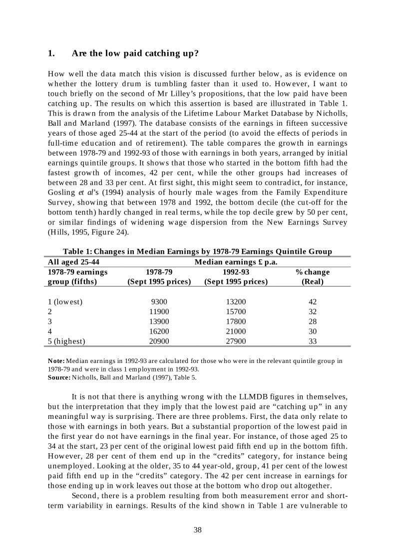
Chapter Three: Does Income Mobility Mean that We Do Not Need to Worry aboutPoverty? 31

John Hills

Chapter Four: Childhood Disadvantage and Intergenerational Transmissions ofEconomic Status 55

Stephen Machin

Chapter Five: Labour Market Flexibility and Skills Acquisition: Is there a trade-off? 65Wiji Arulampalam and Alison L Booth

Chapter Six: Are British Workers Getting More Skilled? 89Frances Green, David Ashton, Brendan Burchell,Bryn Davies and Alan Felstead

iv

List of Contributors

Wiji Arulampalam is Reader in Econometrics at the University of Warwick.

David Ashton is Professor of Economics at the University of Leicester.

A B Atkinson is Warden of Nuffield College, Oxford.

Alison Booth is Professor of Applied Economics, ESRC Research Centre on Micro-Social Change at the University of Essex and Research Fellow of the CEPR.

Andrew Britton was Executive Secretary of the Churches' Enquiry intoUnemployment and the Future of Work and formerly Director of the National Institutefor Economic and Social Research.

Brendan Burchell is a member of the Faculty of Social and Political Sciences at theUniversity of Cambridge.

Bryn Davies is a consultant in occupational psychology.

Alan Felstead is a Senior Research Fellow in the Centre for Labour Market Studies,University of Leicester.

Frances Green is Professor of Economics at the University of Leeds Business School.

John Hills is Professor of Social Policy and Director of the Centre for Analysis ofSocial Exclusion, London School of Economics.

Stephen Machin is Professor of Economics, University College London and aResearch Associate of the Centre for Economic Performance at the London School ofEconomics.

v

Preface

The principal aim of Section F of the British Association is to show how economicanalysis can be applied to illuminate important issues of public concern. The themefor the 1997 Section F Meeting of “Equality and Opportunity” surely satisfied thiscriterion. The subject matter is highly relevant to key initiatives of the LabourGovernment elected in May 1997. The first Budget of Gordon Brown was centred onWelfare to Work, seeking to create employment opportunities for the young and thelong-term unemployed. Training, education, and the acquisition of skills are centralto the Government's programme. In August 1997, Peter Mandelson, Ministerwithout Portfolio, announced that there would be a campaign against socialexclusion as a prominent plank in government policy. December saw theestablishment of the new Social Exclusion Unit. According to the Prime Minister, thisis in many ways “the defining difference between ourselves and the previousgovernment” (The Observer, 23 November 1997).

The measures are yet to take full effect, and it will not be possible to evaluatetheir impact for some time. But we can ask now what one can learn from moderneconomics, together with other social sciences, that is relevant to this policy area. Viewsdiffer as to the contribution of modern economics to understanding contemporaryproblems. Andrew Britton, in his chapter, reaches rather negative conclusions aboutthe contribution of economics. He says that the subject of the Section’s meeting showsup the limitations of economics rather than its strengths. In my contribution, I am moreupbeat. While there are major gaps in our understanding, to a notable degree Britisheconomists have identified the areas where more knowledge is needed, and haveinvested in acquiring data and developing theories.

My Presidential Address, which is Chapter One of this Paper, is concerned withthe three-way relationship between poverty, unemployment and social exclusion.These concepts are related but should not be equated. In debates about Social Europe,the terms poverty and social exclusion have on occasion been used interchangeably,but they are not the same. People may be poor without being socially excluded; andothers may be socially excluded without being poor. Unemployment may causepoverty, but this may be prevented, as in a number of mainland European countries,by social security. In countries such as France there has not been the same rapid rise inpoverty as in the United Kingdom. Unemployment may cause social exclusion, butemployment does not ensure social inclusion; whether or not it does so depends on thequality of the work offered. “Marginal” jobs may be no solution.

The link between employment and social cohesion is the subject of Chapter Twoby Andrew Britton, Executive Secretary of the Churches' Enquiry into Unemploymentand the Future of Work, which reported in April 1997. He argues that conventionaleconomic analysis is too committed to individualism and too narrowly focused on amaterial view of human well-being. It therefore misses an important part of theproblem of unemployment: the role of work in providing self-esteem and a properstate of being. The search for social cohesion in the Report of the Churches' Enquirymay be seen as an application of a social contract, but a Christian approach is onebased on sharing of suffering. The resulting policy recommendations have somecongruence with the approach of the new Government, aiming to ensure enough good

vi

work for all, but there are also major differences. Notably, the Report argues thatpaying taxes is an important way in which we discharge our social obligations, andthat higher taxation is necessary to finance the creation of new opportunities, and newjobs, in fields such as health and education.

A key aspect of social exclusion is that of dynamics. People are excluded not justbecause they are currently without a job or income but because they have littleprospects for the future. Assessment of the extent of social exclusion has therefore togo beyond current status. Mobility in terms of incomes is the subject of Chapter Threeby John Hills, Director of the newly established Centre for Analysis of Social Exclusionat LSE. As he notes, longitudinal data are being used to argue that there is considerablesocial mobility, so that a great deal of poverty may be a one-off event, and that mobilityhad increased with labour market flexibility, so that we need be less concerned aboutthe associated rise in earnings differences. He makes the point that mobility is in part alife-cycle phenomenon. This insight goes back at least to Seebohm Rowntree's study ofYork in 1899, but he and Karen Gardiner have taken the analysis an important stepfurther by characterising different types of trajectory, such as “rising out of poverty” or“blips into poverty”. Their characterised trajectories account for a much higher fractionof households than would be expected on a random basis. His chapter points the wayto a much richer understanding of income dynamics.

By future prospects, we have in mind not only those of the current generationbut also those of their children. Social exclusion may apply across generations.Intergenerational transmission of economic status is the subject of Chapter Four byStephen Machin. Using data from the National Child Development Survey, he findsthat the extent of intergenerational mobility is limited in terms of earnings andeducation, and that there is evidence of asymmetry in that upward mobility from thebottom is more likely than downward mobility from the top. He argues that childhooddisadvantage is an important factor in maintaining immobility of economic statusacross generations. If this is the case, then inequality of outcome today is a cause ofinequality of opportunity in the next generation.

The acquisition of skills is the subject of Chapters Five and Six. WijiArulampalam and Alison Booth in Chapter Five explore the connection betweenlabour market flexibility and work-related training. They find, using data from theBritish Household Panel Survey, that workers on short-term contracts, or not coveredby a union collective agreement, are less likely to be involved in work-related trainingto improve their skills. They suggest that there is a conflict between expanding themore marginal forms of employment and expanding the proportion of workers gettingtraining. Such a finding underlines the importance of the quality of employment.

In Chapter Six, Francis Green and colleagues use evidence from the 1997 SkillsSurvey, and a comparison with the 1986 SCELI survey, to examine what has beenhappening to skills, with particular reference to those actually used in the workplace.The findings show a significant increase in the skills used in Britain, with the increasebeing particularly marked among women. There is greater use of problem-solvingskills, of communication and social skills, and of computing skills. At the same time,the authors emphasise that the findings apply only to those in employment, nothingbeing said about skill acquisition by those not in work.

vii

The chapters in this Paper draw on extensive economic research. A significantpart of this research has been financed by the Economic and Social Research Council,and I end by stressing the importance of this funding, and that from independentfoundations such as the Leverhulme Trust and the Joseph Rowntree Foundation.

Tony AtkinsonJanuary 1998

Chapter One: Social Exclusion, Poverty and Unemployment1

Tony Atkinson

1 Poverty and Social Exclusion

A central theme of the paper is the three-way relationship between poverty,unemployment and social exclusion. These concepts are related but should not beequated. In debates about Social Europe, the terms poverty and social exclusion haveon occasion been used interchangeably. Cynics have suggested that the term ‘socialexclusion’ has been adopted by Brussels to appease previous Conservativegovernments of the United Kingdom, who believed neither that there was poverty inBritain nor that poverty was a proper concern of the European Commission.

Poverty and social exclusion are not, however, the same. By “poverty”, I meanthe dictionary definition of “lack of money or material possessions”. This may gotogether with being “shut out from society” (Tony Blair, 23 November 1997), but itdoes not necessarily do so. People may be poor without being socially excluded in thePrime Minister’s sense. People may be socially excluded without being poor.Confusion of the two concepts is one reason for differences of view about the role ofsocial security benefits.

The three-way relationship between poverty, unemployment and socialexclusion is developed in the next three sections of the paper. A route map is providedby Figure 1. Unemployment may lead to poverty, but it does not necessarily do so(Section 2). Does unemployment lead to social exclusion (Section 4)? To answer this, wehave first to define what we mean by social exclusion (Section 3).

A second theme of this paper is the tension within the European Union betweendifferent approaches to the labour market. We can represent the UK as being in themiddle of a tug of war between American and Continental European conceptions ofthe future of the labour market and the welfare state. On one side, there is increasedlabour market flexibility, which has dominated Anglo-Saxon thinking, and which hasbeen forcefully advocated by the IMF and the OECD. On the other, there is theContinental European approach, which gives more weight to labour market securityand social partnership, and which values the economic contribution of a proper systemof social protection. This over-simplifies the two positions, but the tension is a genuineone.

Reflecting this difference in approach, debates about social exclusion in theUnited Kingdom emphasise the role of workers and families. Increased labour marketflexibility is interpreted by many politicians to be a matter of adjustments by those onthe supply side of the labour market: workers and their representatives. There are,however, other actors who should not be overlooked and whose role has receivedmore attention in Continental debates. The Government itself may contribute to social

1 Presidential Address to Section F of the British Association for the Advancementof Science, Annual Meeting, University of Leeds, September 1997.

10

exclusion where its social security benefit programmes privilege certain groups ofworkers (Section 5). There are those who campaign for more inclusionary benefitschemes, such as a citizen’s income; others argue that the state is too inclusionary andshould be more open to pluralism in both welfare provision and life styles.

A further important class of actors is that of firms. There are two sides to thelabour market, and we need to consider the role of employers, whose labour marketdecisions may contribute to the exclusion of workers (Section 6). A high required rateof return, or a short time horizon, may inhibit employers from taking on new workers.Firms may not be willing to invest in job creation. Examination of firm behaviourbrings us to another dimension of social exclusion: that which occurs in the domain ofconsumption. People may be excluded if they are unable to participate in thecustomary consumption activities of the society in which they live. Their access toconsumer goods and services depends in part on the pricing decisions of firms (Section7). For utilities such as electricity or telephones, the connection of consumers may beinfluenced by regulatory and public sector policy.

Poverty Unemployment

Social Exclusion

Social Exclusion

CompaniesSocialSecurity

2

1 4

5

6

78

3

relativity

agency

dynamics

Figure 1: Route Map (Section numbers)

11

Exclusion from consumption is also a function of income, which takes us backonce more to social security benefits and the determination of benefit levels (Section 8).While poverty is not the same as exclusion, raising people’s incomes via social securityis an essential part of any programme to reduce exclusion. Simply linking benefits toretail prices is not sufficient to guarantee that benefit recipients can continue toparticipate in normal consumption activities. Their exclusion from consumption may inturn limit their capacity to engage in the modern labour market.

2 Unemployment and Poverty

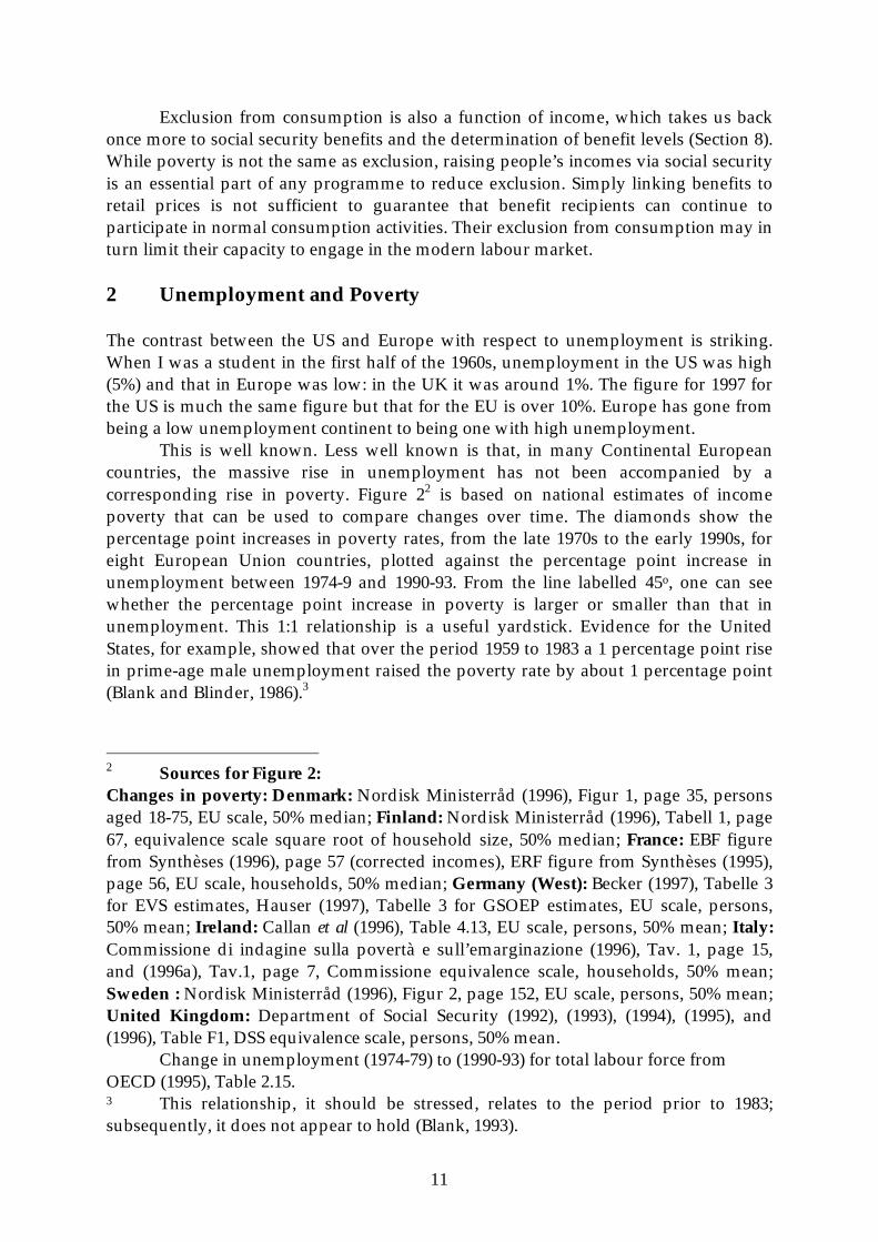
The contrast between the US and Europe with respect to unemployment is striking.When I was a student in the first half of the 1960s, unemployment in the US was high(5%) and that in Europe was low: in the UK it was around 1%. The figure for 1997 forthe US is much the same figure but that for the EU is over 10%. Europe has gone frombeing a low unemployment continent to being one with high unemployment.

This is well known. Less well known is that, in many Continental Europeancountries, the massive rise in unemployment has not been accompanied by acorresponding rise in poverty. Figure 22 is based on national estimates of incomepoverty that can be used to compare changes over time. The diamonds show thepercentage point increases in poverty rates, from the late 1970s to the early 1990s, foreight European Union countries, plotted against the percentage point increase inunemployment between 1974-9 and 1990-93. From the line labelled 45o, one can seewhether the percentage point increase in poverty is larger or smaller than that inunemployment. This 1:1 relationship is a useful yardstick. Evidence for the UnitedStates, for example, showed that over the period 1959 to 1983 a 1 percentage point risein prime-age male unemployment raised the poverty rate by about 1 percentage point(Blank and Blinder, 1986).3

2 Sources for Figure 2:Changes in poverty: Denmark: Nordisk Ministerråd (1996), Figur 1, page 35, personsaged 18-75, EU scale, 50% median; Finland: Nordisk Ministerråd (1996), Tabell 1, page67, equivalence scale square root of household size, 50% median; France: EBF figurefrom Synthèses (1996), page 57 (corrected incomes), ERF figure from Synthèses (1995),page 56, EU scale, households, 50% median; Germany (West): Becker (1997), Tabelle 3for EVS estimates, Hauser (1997), Tabelle 3 for GSOEP estimates, EU scale, persons,50% mean; Ireland: Callan et al (1996), Table 4.13, EU scale, persons, 50% mean; Italy:Commissione di indagine sulla povertà e sull’emarginazione (1996), Tav. 1, page 15,and (1996a), Tav.1, page 7, Commissione equivalence scale, households, 50% mean;Sweden : Nordisk Ministerråd (1996), Figur 2, page 152, EU scale, persons, 50% mean;United Kingdom: Department of Social Security (1992), (1993), (1994), (1995), and(1996), Table F1, DSS equivalence scale, persons, 50% mean.

Change in unemployment (1974-79) to (1990-93) for total labour force fromOECD (1995), Table 2.15.3 This relationship, it should be stressed, relates to the period prior to 1983;subsequently, it does not appear to hold (Blank, 1993).

12

West Germany has close to a 1:1 relationship between unemployment andpoverty; Sweden has a larger increases in poverty than unemployment. But it is the UKwhich stands out: the proportion of people living in households with low incomesmore than doubled over the period when Mrs. Thatcher was Prime Minister (it fell alittle while Mr. Major was Prime Minister).4 In the majority of European countries,however, there has been little or no increase in poverty. Between the late 1970s and theearly 1990s, poverty did not show a trend increase in Denmark, Finland, France orItaly.

The same picture is shown by studies using data from the Luxembourg IncomeStudy. Smeeding (1997) uses a scale of

0 for a change of less than 1 percentage point,+ (or -) for an increase (decrease) of 1 to 2 percentage points,++ (--) for 2 to 4 percentage points,+++ (---) for 4 points or more.

Taking a base year between 1979 and 1981, the UK scored +++ for the change up tothe early 1990s, and the US ++, whereas Sweden and Norway scored +, and France

4 The high quality of statistics in the UK on financial poverty owes a great deal tothe Department of Social Security. The development of the Households Below AverageIncome series (for example, Department of Social Security, 1997) is one of the mostimportant recent developments in official statistics. There is equally a long tradition ofacademic inquiries, from the postwar revival of concern with Abel-Smith andTownsend’s The Poor and the Poorest (1965) to the establishment in October 1997 of theESRC Centre for Analysis of Social Exclusion.

Figure 2 Changes in poverty and increases in unemployment in Europe: late 1970s to early 1990s

-6

-4

-2

0

2

4

6

8

10

12

0 1 2 3 4 5 6 7 8 9

% point increase in unemployment

% p

oin

t ch

ang

e in

po

vert

y Sweden

UK

Germany

Italy

France

Ireland

Finland

Denmark

45 degree line

13

and Spain scored -. For shorter periods, West Germany and the Netherlands scored+, but Belgium, Denmark and Finland scored 0. Smeeding concludes that

trends in poverty in the 1980s were generally flat with the exception of theUnited States and the United Kingdom (1997: 25).

This may suggest that we need not be concerned about unemployment inEurope. However, there is a serious risk, emphasised by Sen (1997), that Europeansbecome complacent about their levels of unemployment. He contrasts attitudes in theUnited States and Europe:

American social ethics finds it possible to be very non-supportive of theindigent and the impoverished, in a way that the typical West European,reared in a welfare state, finds hard to accept. But the same American socialethics would find the double-digit levels of unemployment, common inEurope, to be quite intolerable (1997: 11).

As he, and others such as Clark and Oswald (1994), have stressed, unemploymenthas costs which go beyond the loss of cash income. Even if there were 100%replacement of lost income, individuals would suffer from unemployment.Moreover, it is not only individual welfare which is at stake but also wider objectivessuch as social integration.

At the same time, it does not follow that employment implies social inclusion.People may remain excluded even though at work. This however raises the questionthat I can avoid no longer – what do we mean by social exclusion?

3 The Definition of Social Exclusion

Social exclusion is a term that has come to be widely used, but whose exact meaning isnot always clear. Indeed, it seems to have gained currency in part because it has noprecise definition and means all things to all people. A review of the sociologicalliterature concluded that

Observers in fact only agree on a single point: the impossibility to define thestatus of the ‘excluded’ by a single and unique criterion. Reading numerousenquiries and reports on exclusion reveals a profound confusion amongstexperts (Weinberg and Ruano-Borbalan, 1993, translation by Silver, 1995:59).

There do however seem to be three elements that recur in the discussion. Thefirst is that of relativity. People are excluded from a particular society: it refers to aparticular place and time. In the case of poverty, such relativity has been challenged.According to Joseph and Sumption,

A person who enjoys a standard of living equal to that of a medieval baroncannot be described as poor for the sole reason that he has chanced to beborn into a society where the great majority can live like medieval kings(1979: 27).

However, whatever the merits of an absolute approach when measuring poverty, it hasno relevance to social exclusion. We cannot judge whether or not a person is socially

14

excluded by looking at his or her circumstances in isolation. The concreteimplementation of any criterion for exclusion has to take account of the activities ofothers. People become excluded because of events elsewhere in society. Exclusion mayindeed be a property of groups of individuals rather than of individuals. Economiststend to consider individuals and their families in isolation: for example, taking noaccount of whether the respondents in a sample survey come from the same street orneighbourhood. Yet social exclusion often manifests itself in terms of communitiesrather than individuals, an illustration being the use by financial institutions of streetpostcodes for purposes of credit rating.

This brings me to a second element, which is that of agency. Exclusion implies anact, with an agent or agents. People may exclude themselves in that they drop out ofthe market economy; or they may be excluded by the decisions of banks who do notgive credit, or insurance companies who will not provide cover. People may refuse jobspreferring to live on benefit; or they may be excluded from work by the actions of otherworkers, unions, employers, or government. This notion of agency has been examinedby Sen in his work on social justice, stressing the difference between (1) the realisationof one’s objectives irrespective of one’s own role and (2) their realisation as a result ofone’s own efforts (Sen, 1985 and 1992). Put the other way round, in terms of failure toachieve the status of inclusion, we may be concerned not just with a person’s situation,but also the extent to which he or she is responsible. Unemployed people are excludedbecause they are powerless to change their own lives.

A third key aspect is that of dynamics. People are excluded not just because theyare currently without a job or income but because they have little prospects for thefuture. By “prospects”, we should understand not only their own but also those of theirchildren. Social exclusion may apply across generations. Assessment of the extent ofsocial exclusion has therefore to go beyond current status. The same can be argued ofpoverty, and Robert Walker has argued that this is one way of bringing together thetwo concepts:

when poverty predominantly occurs in long spells ... the poor have virtuallyno chance of escaping from poverty and, therefore, little allegiance to thewider community ... In such a scenario the experience of poverty comesvery close to that of social exclusion (1995: 103).

There is greatly increased risk but the two concepts should not be equated: socialexclusion is not simply long-term, or recurrent, poverty. Social exclusion is not only amatter of ex post trajectories but also of ex ante expectations. We need forward-lookingindicators.

Empirical implementation of measures of social exclusion poses major researchproblems, but the three elements of relativity, agency and dynamics provide a basis forconsidering in principle the mechanisms of exclusion and inclusion that are the subjectof the rest of the paper.

4 Unemployment and Social Exclusion

The 1994 European Union White Paper on Growth, Competitiveness, Employment arguesthat the creation of jobs is necessary to safeguard

15

the future of our children, who must be able to find hope and motivation inthe prospect of participating in economic and social activity (EuropeanCommission, 1994: 3).

Would a fall in unemployment in Europe provide such a guarantee of social inclusion?The answer must depend on the reason for unemployment and on the form

taken by the increase in employment. If unemployment is due to deficiency ofaggregate demand, or technological shifts, then an individual worker may reasonablyfeel that he or she is powerless in the face of macro-economic forces. Studies ofunemployment in the 1930s, such as Bakke (1933) in the United States or Jahoda et al(1933) in Germany, emphasised the loss of personal control; and recent reviews in the1980s

have been impressed more by the similarities than the differences inresearch findings on current unemployment (Lewis et al, 1995: 159).

Reduction of such “involuntary” unemployment would score positively in terms of theagency dimension of exclusion. On the other hand, this presupposes that return towork does in fact restore a sense of personal control. As noted in one summary ofBakke’s research, it

suggested that much of the apparent inactivity and negative mood of theunemployed was not a function of job loss alone. It was also a function ofpast work experiences which left people feeling they lacked control of theirlives (O’Brien, 1986: 195-6).

If, on the other hand, unemployment is attributed to high reservation wages, forexample, on account of the level of unemployment benefit, then again the issue arisesof the nature of the employment which would be generated as a result of policymeasures to reduce unemployment (for example, benefit cuts). Critics of the Americanapproach of labour market flexibility see it as generating jobs which are less privilegedin their remuneration or in their security. The newly created jobs are seen as“marginal” rather than “regular” jobs, where the latter have the expectation ofcontinuing employment, offer training and prospects of internal promotion, and arecovered by employment protection. “Marginal” jobs lack one or more of theseattributes; they may also be low paid. In this respect, the relativity of the concept ofexclusion becomes important. If the expansion of employment is obtained at theexpense of a widening of the gap between those at the bottom of the earnings scale andthe overall average, then it may not end social exclusion.

It is possible that new jobs are marginal, but offer future prospects, which bringsus to the dynamic dimension of exclusion. The key question is whether these jobs are infact stepping-stones to regular employment or whether they trap people in low paidand insecure jobs with recurrent unemployment. Does the young woman who comesin to do part-time photocopying get taken on as a management trainee? Figures 3A and3B show two different stylised situations, where the size of the circles is an indicator ofthe relative probabilities of movement. In Figure 3B, employment in the marginalsector is indeed a stage of transition to regular employment. Workers progress. Havingproved their employability, they stand a good chance of being taken on in a regular job.In terms of the typology in John Hills’ paper in this volume, people are rising out of

16

poverty. On the other hand, in Figure 3A there is little connection between the regularsector and marginal employment/ unemployment. People go up and down at thelower levels of income. Their trajectories are, in Hills’ terminology, repeated poverty orblips out of (into) poverty. This happens independently of the overall rate ofunemployment.

Figure 3A: Social SeparationTo:

From: Regular job Marginal job Unemployment

Regular jobl l l

Marginal jobl l l

Unemploymentl l l

Figure 3B: Stepping Stone MobilityTo:

From: Regular job Marginal job Unemployment

Regular jobl l l

Marginal jobl l l

Unemploymentl l l

Which, if either, of these two pictures is more relevant is an empirical question. Recentresearch has made productive use of longitudinal data, such as those collected in theBritish Household Panel Survey (a far-sighted social science investment which is nowpaying off) to learn about labour market transitions. We have seen a series of veryinteresting studies, including chapters in this volume. Here I simply refer to one study,that by Amanda Gosling et al (1997), which casts light on the transitions out of low paidjobs, where low pay is defined in terms of hourly earnings in the bottom quartile. Thefindings (Gosling et al, 1997, Figure 3.1) indicate that 36% of low paid men in the firstyear of the survey had moved out by the next year, but this included 11% who wereout of work. Of the 25% who moved up the earnings distribution, about 30% revertedto the low paid group in the next year or the following one. This suggests that asignificant number are indeed trapped, although this kind of evidence tends to raise asmany questions as it answers: for example, it is not clear that hourly earnings are anadequate yardstick. As at the top of the scale, it is the total remuneration packagewhich is relevant, including the qualitative features associated with the marginality ofjobs.

The link between employment and social inclusion is a complex one. Creatingjobs can contribute to ending social exclusion, but success depends on the nature of

17

these new jobs. Do they restore a sense of control? Do they provide an acceptablerelative status? Do they offer prospects for the future? These are importantquestions.

18

5 Social Security

In describing the history of use of the word “exclusion” in France, Hilary Silver statesthat

The coining of the term is generally attributed to René Lenoir, who, in 1974... estimated that `the excluded’ made up one-tenth of the Frenchpopulation. ... All were social categories unprotected under social insuranceprinciples at that time (1995: 63).

This brings us to a different source of exclusion: that people are excluded from thewelfare state.

In France, concern with a patent lack of solidarity led to the introduction of theRevenu Minimum d’Insertion. In the UK the situation is different in that a nationalsystem of social assistance has long been in operation (although this has begun to comeunder threat). There are however questions as to how far means-tested benefits can berelied on as a source of inclusion. As is well known, take-up of assistance issignificantly less than 100% (Department of Social Security, 1996a). Incomplete take-upin part reflects lack of information, or the time costs of claiming, but studies of themotives for not claiming reveal that it is also related to stigma associated with receiptof assistance. People do not wish to be identified as recipients of Income Support, andin this regard the benefit system itself is exclusionary. There are also fears that the newgovernment measures stressing return to work will stigmatise those who remain onbenefits, making them feel excluded by the state. There are serious dangers in stressingthe negative aspects of welfare receipt. Headlines such as “The £X million Scandal of‘Skivers’” do not help.

Consideration of the role of the state may lead to more fundamentalquestioning. Goodin has argued that there is a sense in which

the state, as presently conceived, is too inclusive. It is not necessarily itself theonly source of social succour available to any given citizen. But it claims amonopoly on the power to legitimate any other sources of social succour(1996: 363).

He puts forward an alternative model in which

we could be members of many different clubs, drawing on them in turn formany different purposes and many different kinds of support andassistance (1996: 364).

The European Union is, he suggests, a prototype of such an organisation. It is anintriguing thought that exclusion at a national scale might be resolved at a Europeanlevel. Political realities indicate that access to Brussels may be even more difficult forthose on margins of society, but the European Poverty Programmes have beenexplicitly concerned with the fostering of economic and social integration of under-privileged groups (see for example Duffy, 1994).

These considerations point to a rather different agenda from that usuallyenvisaged under the slogan of “rethinking the welfare state”, but they should not betaken as implying that national social security has no role to play in combatting socialexclusion - to which I return in Section 8.

19

6 Role of Employers

In his Presidential Address to Section F in 1958, Professor Arthur Brown, seeking toexplain how the postwar decade had come to surpass the hopes of Lord Beveridgewith regard to unemployment, noted

one factor which was imperfectly foreseen, and which may have played avery important part in realising the still lower level of unemployment whichwe have reached. That factor is a change in the attitude of employers, fromregarding labour as a commodity always in elastic supply to treating it assomething which, if once released, may not be easily replaced (1958: 450).

The role of employers is, in my view, too little emphasised in today’s economicanalysis. In seeking to explain the rise in unemployment, we have to consider thehiring decisions of employers. Are people now being excluded from the labour marketby the employment practices of companies?

To illustrate this, let us return to the explanation of unemployment, in this casetaking a simple model of equilibrium employment based on matching ofvacancies/unemployed and bilateral wage bargaining, jobs are created until

Marginal return to labour =Reservation wage

+ Cost of job creation * (Rate of job termination + Rate of discount) / Employer’srelative bargaining power

Employment is expanded up to the point where the marginal return is equal to theright hand side. The left and side falls as employment increases, so that the larger theright hand side the lower is employment.

From this, we can see the basis for the labour flexibility argument referred toearlier. Cutting social security benefits, it is argued, reduces the reservation wage, andhence expands employment. Reducing hiring costs expands employment. Reducingtrade union power, and hence increasing that of the employers, increases employment.This however focuses on the side of labour supply. Attention needs to be directed notjust at workers and unemployed but also at employers. How do firms influence jobcreation and job destruction? If, for instance, employers now expect jobs to be short-lived, anticipating a high rate of termination, this raises the right hand side, making jobcreation less attractive. Perhaps most importantly, if employers are applying a higherrate of discount to future benefits, then they are less willing to invest in job creation.Debate about “short-termism” should not be confined to the capital market; it may beequally relevant to the labour market.

In this way, we are led to link social exclusion with the capital market, bringingit closer to the heart of economic analysis. The next step is to bring in the productmarket.

7 Social Exclusion in Consumption

20

Social exclusion has so far been equated with exclusion from the labour market, but it isonly one face of social exclusion. People may face exclusion in other parts of their lives,notably in the domain of consumption. An important strand in the concerns that havebeen expressed is that people are unable to participate in the customary consumptionactivities of the society in which they live. The most evident example is that ofhomelessness, but also significant are access to durables, food expenditure (nutritionalcontent), and expenditure relating to recreational, cultural and leisure activities. Thelast of these is particularly relevant to families with children. Peer group pressure maymean that a Manchester United shirt or Nike trainers are necessary for children to beincluded in neighbourhood activities.

Exclusion may apply not just to goods but also to services. The poor may beexcluded from insurance cover where premia are set on a postcode basis; banks mayrefuse on similar criteria to open bank accounts or to issue credit cards. The services arenot available locally:

Using computerised mapping technology to show where profits are highest,banks and building societies have been pulling out of poorer areas. [Forexample] all the building society branches have closed in Birmingham’sAston ward since 1986 (Rossiter and Kenway, 1997: 7).

Such credit-rating criteria may be a rational response on the part of financialinstitutions, but this does not change the consequences for individual families.According to McCormick (1997), when a low income housing estate in Scotlandsuffered flooding in the winter of 1994, 95 per cent of the tenants were not insured.

A good example of exclusion in consumption is the telephone. A person unableto afford a telephone finds it difficult to participate in a society where the majority havetelephones. Children are not invited out to play, because neighbours no longer callround - they call up. Letters do not allow the same contact to be kept with relativeswho have moved away. A person applying for a job may not be called for interviewsince he or she cannot be contacted directly. This may sound like an advertisement forthe telephone companies, but it is to them, and other suppliers of key goods andservices, that I would like to direct attention. The conditions under which goods aresupplied is an aspect which is overlooked in the analysis of poverty. The pricingdecisions of the suppliers determine whether or not the poor are excluded from thisdimension of consumption. If one examines the choices made by profit maximizingfirms (Atkinson, 1995), then it is quite possible that the profit-maximizing priceexcludes some customers from the market. Equally, there is no guarantee that firmswill go on supplying the qualities of goods that the poor want to buy. For example, it isnot now easy to buy small quantities of foodstuffs, or cheap cuts of meat.

Exclusion of consumers is a particular issue where the supply of the good orservice has passed from public to private hands. This raises questions to do withregulation – the subject of last year’s Section F meeting. Whereas the government couldrequire public enterprises to choose their tariffs in such a way that households living onIncome Support can afford electricity or gas, or to travel to work, privatisation requiresthat some mechanism be put in place to avoid exclusion of low income customers bythe new profit maximising management. Where the industry is regulated, then theregulators can impose an access condition. The United Kingdom privatisationlegislation contains an obligation to supply “all reasonable demands”, but this is open

21

to a variety of interpretations, and some deny that social exclusion is an appropriateconsideration. According to John Vickers,

the advantages of regulators having discretion to pursue distributional endsare outweighed by disadvantages of capture, influence activities,uncertainty, and unaccountability (Vickers, 1997: 18).

This is not apparent to me. The risks of political influence arise not just with regulationbut also with taxes and transfers. Fiscal policy may be “captured”, preventing agovernment from using redistributive taxes and benefits. One has to balance the twosides.

The potential seriousness of consumer exclusion is illustrated by the UK gasindustry. Ruth Hancock and Catherine Waddams Price (1995) have examined theimpact by income groups of the reductions in gas tariffs for those who pay by directdebit. A larger proportion in the top quintile already pay by direct debit and of theremainder almost all have bank accounts, so that they can take advantage of thepreferential tariff. In the bottom quintile a sizeable proportion do not have bankaccounts. What this points to is the risk of multiple exclusion, where people are unableto open a bank account and are thereby unable to avoid paying by more expensive slotmeters.

The policy of utility suppliers is also relevant to the determination of socialsecurity benefits, which brings me back to this subject.

8 Social Security Cannot be Left Out

Results from the recent literature on the economics of industrial organisation can beused to illuminate the problem of regulation just discussed. They also point to theinterdependence between the living standards of the poor and those of the society inwhich they live. From models of firm decisions about pricing and about the qualitiessupplied, it can be seen that in the long-run the price of goods rises as incomes rise inthe community in general. As the bulk of the population becomes richer, so the poorneed more income to keep up. Firms no longer find it profitable for example toproduce goods of lower quality, when the rest of the population has moved “upmarket”.

This has evident implications for benefit levels. Linking benefits to the generalprice index may be insufficient to prevent people from being excluded from theconsumption of key goods and services. As the rest of the population becomes richer,there is a rise in the minimum income needed to participate. For example to competefor a job, it is today not enough to “avoid being shabby”, which was the criterionapplied by Seebohm Rowntree in 1899. To keep up at school, children need a range ofgoods which was inconceivable even fifty years ago. This may mean that benefits allowpeople to purchase a better basket of goods than in 1949, but this is what is necessary toavoid exclusion. And it would not be possible to purchase the 1949 basket, since not allthe goods are available in today’s richer society.

The role of benefits should be stressed, since present Government policy isfocussed so exclusively on the labour market. Income from work is important butcannot be the sole solution. As discussed in Section 5, the form of social security needs

22

to be reconsidered, but collective provision - whether social insurance or citizen’sincome or participation income - seems essential to assure social integration.

Conclusions

In this paper, I have ranged widely; and indeed this is one of the main conclusions.Social exclusion is not just concerned with unemployment. People may be excludedfrom participation in today’s society by the operations of the state: for example,through the use of means tested benefits that are seen as stigmatizing. People may beexcluded by the pricing and other decisions of the suppliers of key goods and services.By the same token, government policy has to take a broad view. The setting up of theinter-departmental Social Exclusion Unit (Mandelson, 1997) is indeed the right way togo. Social exclusion is not just a matter for one government department. All policyproposals should be tested against the contribution that they make to promoting socialinclusion.

The second conclusion is that government policy can make a difference. It is notthe case that social exclusion is simply the product of world economic forces in the faceof which the government is powerless. The government can make interventions in thelabour market of the kind which have been announced under the heading of Welfare toWork, but the scope of policy should be broader. Employment in itself is not necessaryinclusionary; the quality of the new jobs is also important. Policies of labour marketflexibility may simply shift people from unemployment to marginal jobs with noprospects. The role of employers in job destruction and job creation needs to beconsidered. Labour market measures should not be seen as an alternative to socialtransfers; these policies are complementary. The form of social security needs to be re-considered from the standpoint of social exclusion, but it will remain important evenwith improved labour market opportunities. And there are other areas of policy whichneed to be reviewed. The government can intervene in the tariff policy of privatisedutilities, such as gas, which may prevent people from having access to essentialservices.

The third conclusion is that economic analysis, for all its limitations, does have auseful role to play in illuminating the different elements of social exclusion. Theflowering of empirical research using longitudinal data has come just at the right timeto help understand the processes that determine how people escape, or do not escape,from social exclusion (“dynamics”). The analysis of employment determination castslight on the “agency” by which people are excluded. Models of decisions by firmsabout pricing show how people are excluded from consumption and demonstrate the“relativity” of the concept.

23

References

Abel-Smith, B, and Townsend, P (1965), The Poor and the Poorest, London: Bell.Atkinson, A B (1995), “Capabilities, exclusion, and the supply of goods” in K Basu, P

Pattanaik and K Suzumura (eds), Choice, Welfare, and Development, Oxford:Clarendon Press.

Bakke, E (1933), The Unemployed Man, London: Nisbett.Becker, I (1997), “Die Entwicklung von Einkommensverteilung und der

Einkommensarmut in den alten Bundesländern von 1962 bis 1988” in Becker, Iand Hauser, R, Einkommensverteilung und Armut, Frankfurt am Main: CampusVerlag.

Blank, R M (1993), “Why were Poverty Rates so High in the 1980s?”, in Papadimitriou,D B, and Wolff, E N (eds), Poverty and Prosperity in the USA in the Late TwentiethCentury, Basingstoke: Macmillan.

Blank, R M, and Blinder, A S (1986), “Macroeconomics, Income Distribution, andPoverty”, in Danziger, S H, and Weinberg, D H (eds), Fighting Poverty,Cambridge, Massachusetts: Harvard University Press.

Brown, A J (1958), “Inflation and the British Economy”, Economic Journal, 68: 449-463.Callan, T, Nolan, B, Whelan, B J, Whelan, C T and Williams, J (1996), Poverty in the

1990s, Dublin: Oak Tree Press.Clark, A E and Oswald, A (1994), “Unhappiness and Unemployment”, Economic

Journal, 104: 648-659.Commissione di indagine sulla povertà e sull’emarginazione (1996), La Povertà in Italia

1980-1994, Rome: Presidenza del Consiglio dei Ministri.Commissione di indagine sulla povertà e sull’emarginazione (1996a), La Povertà in Italia

1995, Rome: Presidenza del Consiglio dei Ministri.Department of Social Security (1992), Households Below Average Income: A Statistical

Analysis 1979 - 1988/89, London: HMSO.Department of Social Security (1993), Households Below Average Income: A Statistical

Analysis 1979 - 1990/91, London: HMSO.Department of Social Security (1994), Households Below Average Income: A Statistical

Analysis 1979 - 1991/92, London: HMSO.Department of Social Security (1995), Households Below Average Income: A Statistical

Analysis 1979 - 1992/93, London: HMSO.Department of Social Security (1996), Households Below Average Income: A Statistical

Analysis 1979 - 1993/94, London: HMSO.Department of Social Security (1996a), Income Related Benefits Estimates of Take-Up in

1994/95, London: Government Statistical Service.Department of Social Security (1997), Households Below Average Income: A Statistical

Analysis 1979 - 1994/95, London: HMSO.Duffy, K (1994), “Submission to Sub-Committee C, House of Lords, Regarding the UK

Dimension of the Third European Programme”, University of Warwick.European Commission (1994), Growth, Competitiveness, Employment, Brussels.Goodin, R (1996), “Inclusion and Exclusion”, Archives Européenes de Sociologie, 37: 343-

371.

24

Gosling, A, Johnson, P, McCrae, J, and Paull, G (1997), The Dynamics of Low Pay andUnemployment in Early 1990s Britain, London: Institute for Fiscal Studies.

Hancock, R, and Waddams Price, C (1995), “Competition in the British domestic gasmarket: efficiency and equity”, Fiscal Studies, 16(3): 81-105.

Hauser, R (1997), “Vergleichende Analyse der Einkommensverteilung und derEinkommensarmut in den alten und neuen Bundesländern von 1990 bis 1995”in Becker, I and Hauser, R, Einkommensverteilung und Armut, Frankfurt am Main:Campus Verlag.

Jahoda, M, Lazarsfeld, P F, and Zeisel, H (1933), Marienthal, English translationpublished 1972 by Tavistock Publications, London.

Joseph, Sir Keith, and Sumption, J (1979), Equality, London: John Murray.Mandelson, P (1997), Labour’s next steps: tackling social exclusion, Fabian Pamphlet 581,

London.McCormick, J (1997), “Insuring on a Low Income”, IPPR in Progress, Spring: 3-4.Nordisk Ministerråd (1996), Den nordiska fattigdomens utveckling och struktur,

Copenhagen: Tema-Nord.O’Brien, G (1986), Psychology of Work and Unemployment, Chichester: Wiley.OECD (1995), Historical Statistics 1960-1993, Paris: OECD.Rossiter, J and Kenway, P (1997), “Introduction” to Rossiter, J (ed), Financial Exclusion:

Can Mutuality Fill the Gap?, London: New Policy Institute.Sen, A K (1985), “Well-being, Agency and Freedom: the Dewey Lectures 1984”, Journal

of Philosphy, 82: 169-221.Sen, A K (1992), Inequality Re-Examined, Cambridge: Harvard University Press.Sen, A K (1997), “Inequality, Unemployment and Contemporary Europe”,

Development Economics Research Programme Discussion Paper DERP/7,London School of Economics.

Silver, H (1995), “Reconceptualizing social disadvantage: Three paradigms of socialexclusion”, in Rodgers, G, Gore, C and Figueiredo, J B (eds), Social Exclusion:Rhetoric, Reality, Responses, Geneva: ILO.

Smeeding, T M (1997), “Financial Poverty in Developed Countries: The Evidence fromLIS - Final Report to the UNDP”, LIS Working Paper 155.

Synthèses (1995), No 1, Revenus et Patrimoine des Ménages, Paris: INSEE.Synthèses (1996), No 5, Revenus et Patrimoine des Ménages, Paris: INSEE.Vickers, J (1997), “Regulation, Competition, and the Structure of Prices”, Oxford Review

of Economic Policy, 13(1): 15-26.Walker, R (1995), “The dynamics of poverty and social exclusion” in Room, G (ed),

Beyond the Threshold, Bristol: Policy Press.Weinberg, A and Ruano-Borbalan, J-C (1993), “Comprendre l’exclusion”, Sciences

Humaines, 28: 12-15.

25

Chapter Two: Employment and Social Cohesion

Andrew Britton

Introduction

The enquiry was conducted under the auspices of the Council of Churches forBritain and Ireland, with support from all the main Christian denominations. Ourreport5 was published in April of this year and received considerable publicity, notleast because it appeared shortly before the general election and criticised all themain political parties for ignoring the problems of those in the greatest need.

This was not just another report on the economics of employment to add to themany which have been written in recent years.6 The sponsoring group of churchleaders asked for a report which “offers a theological exploration of issues” and“analyses the various emerging trends and evaluates the policy options from aChristian standpoint”. Nevertheless they appointed a professional economist, with abackground in academic research and government service to be the secretary of theworking party and the main author of the report. In this paper I shall reflect on myexperience in discharging that commission. What is it like to work as an economistfor a church organisation? Can economics and theology engage in a fruitfuldialogue? In particular how can they come together to address the issues of equalityand opportunity which are the subject matter of this book?

Economics has been described7 as “the most influential branch of seculartheology”. This should warn us that economics is not quite like the other academicdisciplines represented here at the annual festival of science. The subject matterstudied by most economists is, of course, peculiar to their branch of science, but thatis not their only distinguishing feature. A recent collection of papers by economistsof the Chicago school8 began like this.

Contemporary economists believe that economics is not defined by itssubject matter but by its method. Economists try to understand andexplain the world by assuming that the phenomena they observe are theoutcome of people’s purposeful decisions. Individuals try to achieve theirobjectives, given their limitations - limited time, money and energy - thatis to say they optimise. The interactions of individuals will determinesocial outcomes - that is market equilibrium.

5 Unemployment and the Future of Work - An Enquiry for the Churches, available from bookshops orfrom CCBI Publications, Inter-Church House, 35-41 Lower Marsh, London SE1 7RL.6 For example, OECD (1994), The Jobs Study; European Commission (1993), GrowthCompetitiveness and Employment; Philpott, J (1994), Looking forward to Full Employment, EPI; and Britton,A (1996), The Goal of Full Employment, NIESR.7 Hobsbawm, E, The Age of Extremes, p.547-8.8 Tommasi, M and Ierulli, S, (1995), The New Economics of Human Behaviour, CambridgeUniversity Press.

26

Economists are defined in this quotation as subscribing to a particular philosophicalview of human nature and behaviour, different from that of some other socialscientists. It could well be called a doctrine.

Oddly enough, many theologians at the same time are becoming lessdoctrinaire in the traditional sense of that word. You do not now, for example, haveto believe in God to be an academic theologian. Some “liberation theologians”appear to equate doing theology with political activism rather than thecontemplation of eternal truths. The point of this paper, however, is to argue that aChristian view of human nature must be different from that assumed by mosteconomists. This is especially the case when they discuss policy questions like thoserelating to employment and social cohesion. It is very important, I believe forprofessional economists to realise that not everyone thinks like they do.

I will begin with some general remarks about the relations of positive andnormative questions in economics and in Christian belief. As we shall see thedistinction between ends and means usually made in discussing economic policy isfar from straightforward. I will then describe how economists approach issues ofemployment and social cohesion, offering in both cases a Christian critique.Following on from that I will summarise the main policy conclusions of thechurches’ report, before offering a few related conclusions of my own.

Ends and Means

Students of economics are told that they should distinguish sharply betweennormative questions (what should be?) and positive questions (what is?). However,more philosophically-minded economists recognise that the methods they followoften conflate the two. A recent study written jointly by a philosopher and aneconomist9 concludes as follows:

Unlike the natural sciences, positive economics explains choices in terms ofreasons. Consequently, it cannot avoid depicting human beings as to someextent rational. It cannot avoid raising evaluative questions about thereasons it cites to explain choices, and it cannot avoid suggesting answers tothem.

Thus a dialogue between economics and theology cannot be conducted on thebasis that theology provides the value judgements whilst economics explains what ispossible. Economic theory has some value judgements already implicit in itsmethod. Moreover, theology is by no means confined to questions of value. It laysclaim to knowledge of the state of the world as well. The Christian faith andtraditions have a great deal to say about human nature and about the social andphysical worlds in which we live. This teaching contrasts sharply with some of theassumptions made by economists.

Christian teaching agrees with economic theory that human behaviour can beexplained as the result of rational choices, but it challenges the assumption thatindividual preferences are fixed. On the contrary, it calls for repentance, conversion 9 Hausman, D and McPherson, M (1996), Economic Analysis and Moral Philosophy, CambridgeUniversity Press.

27

and even rebirth. It challenges the methodological individualism which says thatgroups have no identity beyond that of their members - the church after all claims tobe the body of Christ. It also challenges common notions of scarcity with storiesabout the superabundance of bread or wine or fishes. These are all disagreementsabout how the world actually is, not about how we would like it to be.

I was educated as an economist to see my role as a kind of engineering. I wasan expert who could in principle sell his services to any client. I could say to thegovernment, or for that matter the church, “show me your social welfare function”,and then I could go away and work out what advice to give them. I now recognisethat this model of economics will not quite do. Governments are reluctant todescribe their priorities in the form economists would ideally wish. In fact they arereluctant to discuss hypothetical outcomes at all. Whatever the reason may be forthis reticence in governments, I am quite clear that the church does not have a socialwelfare function at all.

Christians are not just concerned about outcomes. They are also, perhaps more,concerned about procedures and motives. They believe in justice and compassion.Procedural justice is at least as important as the justice of the consequences whichfollow. The value of a charitable gift resides in the cost to the giver rather than thebenefit to the recipient - as the story of the widow’s mite illustrates.

There is need for a new and different kind of dialogue between disciplines.Economics has much to contribute to theology, not least its respect for rationalityand human freedom. Conversely, theology has much to contribute to economics,including a much wider appreciation of human motivation and potential. It is notgood enough to say that the two disciplines deal with different spheres of humanlife. That would risk relegating Christianity to a private world of religiosity, treatingfaith as an escape from the world and not as a means of redeeming it.

Chemists distinguish between mixtures and compounds. Most attempts tointegrate economics with theology can at best be called mixtures. The temptation inpreparing a report for the churches on unemployment was to write a separatetheological chapter, which many readers would then skip over. In fact weintroduced some theology throughout the report making it an integral part of theargument. We were aiming to produce a kind of chemical reaction. I would notclaim that we were always successful, but I do think the effort was worthwhile. Inthe end there should be a kind of Christian economics. This paper is another smallstep in that direction.

Employment

Structural unemployment of the kind experienced in most advanced economiessince about 1970 can be viewed as a shocking waste of resources. In variouscountries something between 5 and 20 per cent of the potential labour force is leftidle, even though it would be perfectly willing to work at the going rate of pay. Totaloutput of goods and services is being reduced by a comparable proportion, andeveryone in society is poorer as a result. How has this come about?

One kind of explanation blames rigidities and distortions in the market forlabour. New technology and new patterns of trade are destroying jobs all the time,

28

but the market should be creating new jobs to replace them. But this requires aflexible response: the wages of some jobs should fall if the demand for that kind oflabour has been reduced, whilst the wages for other jobs should rise so that supplywill rise to match demand.

Generally the trend is towards more demand for well-educated and well-motivated people, away from those capable only of routine or low-skilled work. Ifunemployment is to be minimised the market solution is for wage differentials to getwider. That is indeed what has been happening, most of all in America whereunemployment has remained relatively low, much less in Continental Europe whereunemployment is at its highest. In this economic model of the labour market theexistence of powerful trades unions, and even the provision of Income Support tothe unemployed, are seen as distortions preventing the labour market fromachieving an equilibrium.

Economists as a rule favour market solutions to problems like this. They wantto ensure that unemployed people have access to the labour market so that they cancompete effectively for the jobs that are available. In the process they may bid downthe going rate of wages, but that is better than allowing the harmful distortions toremain - or so we are told. The unemployed must be given the incentive to seekenergetically for work - hence the Jobseeker’s Allowance. If that is not enough thenemployers should be offered temporary subsidies to take on the long-termunemployed in preference to other workers, so that they can get back into circulationas it were - hence the New Deal of the new government. This is all about improvedopportunities, one of the key words in the new policy consensus, and one of the keywords in this book.

A Christian economics of unemployment would have a different emphasis.Christians see work in terms of creativity, like the creative work of God. They alsosee work as service, meeting the needs of one another and often getting involvedwith one another as persons, not only as providers and customers. As it happens,this view of work may well be a better guide to the future than can be found in moreconventional economics.

Machines are taking over more and more of the mechanical aspects of work,whether physical or mental. According to a recent American bestseller,10 “Now forthe first time, human labour is being systematically eliminated from the productionprocess”. This is an exaggeration, but to the extent that it is true it applies to labourin activities like agriculture, manufacturing or transport. These were the mostimportant sources of employment in the 19th and 20th centuries, when classical andneo-classical economics was developed. The same considerations do not apply to themainly service-sector employment we can expect in the 21st century.

A young man, speaking of his own experience of unemployment to thechurches’ enquiry, said that it “destroys your spirit”. This is one aspect of theunemployment problem totally missed by a conventional economic analysis.Ridiculous as it may be, conventional economics equates unemployment to leisure.Social psychologists know better than that,11 recognising the destructive effect thatunemployment can have on people’s self-esteem. But even so this misses a crucial 10 Rifkin, J (1995), The End of Work, Putnam.11 See, for example, Argyle, M (1989), The Social Psychology of Work, Penguin.

29

dimension. For the Christian to work is to pray. Hence unemployment not onlythreatens our relationship with society but also deprives us of a means to expressour gratitude to God.

The best analogy for unemployment could be that of disease. The mentalanguish which many of those affected suffer is a symptom of a malfunction in asocial relationship. The task of the economist is to find a cure. Typically, Christiantradition sees human well-being in terms of health rather than wealth. The aim ofpolicy action should not be to maximise some objective function, as welfareeconomists might put it. It is simply to restore the individual and society to theirproper state of being. In the present context that means full employment, or as weput it in the report, “enough good work for everyone”.

Social Cohesion

There is a branch of economics which deals with inequality, a branch to which ourPresident, Tony Atkinson, has made a particularly important contribution. But why,one might ask, should an economist care about inequality at all? Conventionaleconomic theory assumes that the welfare of each individual depends on thesatisfaction of his or her own preferences. Why should preferences depend on thedistribution of goods and services available to people other than myself - andperhaps a few close friends or relations? In economic theory there is, to quote amemorable pronouncement, no such thing as society, and a term like “socialcohesion” has no real meaning at all.

Some economists are utilitarians, in the strict old-fashioned sense of the word.The right thing to do in any situation, they would say, is to achieve the greatest goodfor the greatest number. How the utility of many individuals is to be added up to ameasure of total well-being remains problematic. However, it is plausible to assumethat a pound given to a poor person will do more good than a pound given to a richperson. Hence one kind of welfare economics produces a simple justification forequalising incomes wherever this can be done without reducing the total resourcesavailable for distribution.

The issue of equality does not only arise in a utilitarian context. It is implicit inmuch of political and social ethics. To quote again from the recent study12 ofeconomics and moral philosophy:

Appeals to equality play a crucial role in discussions of economic policy.Welfare-state programs have attempted to diminish inequalities in incomeand status, and concerns about inequalities constitute the main groundsupon which interferences with market outcomes have been defended. Tounderstand whether such programs are advisable, one needs to understandwhat (if any) sort of equality can be a moral ideal.

Some economists are attracted to the political theories of John Rawls.13 He usedthe familiar myth of a social contract, but he said that it should be drawn up so as tomaximise the welfare of the least favoured member of society. This was on the 12 Hausman and McPherson, op.cit., p.135.13 Rawls, J (1971), A Theory of Justice.

30

grounds that a fair social contract must be one in which the contracting parties didnot know in advance what position they would occupy in the resulting society. Risk-averse individuals would play safe by adopting an egalitarian constitution.

All this theorising is based on the assumption of methodological individualismwhich Christian teaching decisively rejects. For Christians the whole body of thechurch is as real as its individual members - possibly more so. In the Bible nationsare personified; they make moral choices and face judgement collectively. “We,being many, are one body…”

This is the sort of language that many economists find difficult to accept. Theywould regard it as “mystical” or “theological”, in the pejorative sense of such words.Some natural scientists may react in the same way. But the programme ofreductionism can be taken too far even in the physical sciences, and certainly insocial science.

There are sometimes simple and elegant relationships describing groupbehaviour; to insist on reducing everything to its constituent parts may result inexplanations which are clumsy and unnecessarily complicated. This applies to thebehaviour of economic units such as companies, trades unions and nationalgovernments. The choices of both producers and consumers can often be bestunderstood by reference to the social groupings to which they belong. Perhaps thereal motive for dogmatic individualism is not scientific at all. Perhaps there is aquasi-religious inspiration behind it, that religion being the worship of the humanwill.

Christians see too great inequality as a threat to the unity of society, or perhapsas a sign that the bonds which hold society together have already been weakened.This is true of extremes of wealth as well as extremes of poverty. In our report weworry about pay at the top being too high as well as about pay at the bottom beingtoo low. Ultimately what is valued is not equality as such but the mutual love andfellowship which it ought to express. Equality which resulted from coercion wouldhave little merit. Those who seek equality out of envy rather than out of good willdeserve no support at all.

Superficially some passages in our report may sound as if they were written byRawlsians. We say, for example:

We should look at unemployment and the future of work particularly fromthe viewpoint of the poor and the powerless themselves… As Christians weare called to listen to what they are saying and to pass the message on.

There is indeed a sense in which Christians always should take the side of thepoor and the weak against the rich and powerful. But this has nothing at all to dowith a mythical social contract. It has to be an expression of active sympathy orcompassion, in other words a sharing in the suffering, and a willingness, to do all wecan to remove the cause of the pain.

Policy Conclusions of the Report

31

The report was written on behalf of the working part as a whole. In practice it waseasier to reach agreement as to what our conclusions should be than it was to agreewhat was the reasoning behind them!

In our report we summarised our policy findings as follows:

The combination of policies most likely to achieve this aim (i.e. Enoughgood work for all) includes:

• reform of the tax system to encourage much more employment in the privatesector;

• much more employment in the public sector, financed by higher taxation;• a programme creating good jobs for the long-term unemployed;• a national minimum wage;• better conditions of work and fairer bargaining over pay;• reform of social security benefits to reduce reliance on means-testing;• giving priority in the education system to basic skills for all young people;• a national employment forum at which such policies could be debated by all

interested parties.Probably the most controversial of these, especially since the election of the

new government, is the second. More public spending can be justified in quiteconventional terms. We need to expand the service sector to create more good jobs asthe demand for labour elsewhere is reduced by new technology or competition fromimports. But much of the service sector - for example, health and education - isdependent on public expenditure. Short of wholesale transfer of these services toprivate funding, there is only one answer - higher taxation.

That is the main argument developed in support of our conclusion in thereport. There is, however, one passage where a rather different voice is heard:

One view, with which we sympathise, is that paying taxes is a way ofdischarging (in some part) our obligation to meet the needs of our nationalcommunity as a whole, and especially the needs of its less fortunatemembers. The origin of that obligation can be attributed either to love or tojustice - to compassion for those in need or to a duty to share God’s giftsmore fairly. A case for redistributive taxation can be constructed on eitherbase. These arguments are not heard often enough today.

In any debate about opportunity and equality this is surely one issue that needs to beaired.

The main findings of our the report are addressed to the government. This istypical of reports of this kind. There is a danger that they degenerate into tediousshopping lists. I hope that we have kept that tendency under control! In fact, weknow that we should not put too much trust in any government to heal the ills of oursociety. It is not just our political leaders who need to repent.

Economists too often assume that everyone in the private sector is motivatedby narrow self-interest while the government is always high-minded and altruistic.This way of approaching policy issues comes all too naturally to one like myself whohas been in the pay of governments for much of his working life! But governmentshave to take account of what the voters want and what industry and the City will

32

accept. The churches are not constrained in this way. Hence our report is addressedto society as a whole, in the hope of influencing public opinion. Only then is it likelythat governments, employers and others in positions of power and responsibilitywill feel able to do what we believe the situation requires.

33

Conclusions

I end with some brief conclusions of my own. The subject of this book, “Equality andOpportunity” shows up the weaknesses of economics rather than its strengths.Economics does not have much purchase on the real issues evoked by those words.As a discipline it is too deeply committed to individualism and to a narrowlymaterial view of human well-being. Fortunately, Christianity, although its influenceon the majority of this country is now quite tenuous, offers an alternative perspectivewhich does address the questions people actually want to ask. People in general dorecognise the social and spiritual significance of work; and they really do want tobelong to a cohesive society. It is not only Christians who say these things, butChristians say them with particular conviction because they belong naturally withfaith in Christ.

I have raised some very broad issues in this paper about the relationshipbetween economic theory and Christian belief, issues which remain unresolved andlargely unexplored. Further dialogue, based on mutual respect, between thedisciplines of economics and theology could well prove fruitful.

34

Chapter Three: Does Income Mobility Mean That We Do NotNeed To Worry About Poverty?

John Hills14

In October 1997, a new research centre, funded by the Economic and Social ResearchCouncil, began work at the London School of Economics. We are called the Centrefor Analysis of Social Exclusion, but our focus will also be on understanding theprevention of exclusion and promotion of inclusion. “Social exclusion” is obviously avogue phrase at the moment, with the establishment of the Government’s SocialExclusion Unit, and the appearance of the phrase in political speeches during the lastfew months. However, the phrase is more useful than simply being a euphemism for“poverty”. As Tony Atkinson explains in his paper, it embodies the ideas of dynamicsand process. As part of the work of the new centre, we would like to understand whysome people’s lives follow one set of trajectories, while others follow different ones.

The emergence of the phrase in British political discourse and theestablishment of the new centre reflect the coincidence of three factors:• Policy interest in a “hand-up” rather than a “hand-out” approach, or in

“pathways out of poverty” as the late John Smith put it. Policymakers maythink that it could be cheaper to intervene at exactly the right moment to turnsomeone’s trajectory around rather than simply giving more cash to those whoare poor at any one time. On the other hand, it might, of course, cost more inthe short-term, at least, if really changing someone’s trajectory involvedsubstantial investment in education, training, and so on.

• Data availability. After a comparative dearth of longitudinal data, researchersnow have access to an increasingly rich set of British longitudinal datasetsincluding: the British Household Panel Survey (BHPS); the National ChildDevelopment Survey (NCDS) and the 1970 Birth Cohort Study (BCS 70); andthe Lifetime Labour Market Database (LLMDB), and other panel data drawnfrom the New Earnings Survey (NES).

• In addition, there is perhaps greater understanding on the part of researchersthat, for instance, “one-off” poverty is a different phenomenon from persistentor repeated poverty. Isolated observations of low income may reflect atemporary gap between jobs; a relatively short period for young people whoseincomes will later rise; or even errors in the data. This difference hasimplications both for the seriousness of the problem and for appropriate policyresponses. Indeed, if all poverty was accounted for by one-off “blips”, maybewe would not need to worry about it very much at all.

14 The author is very grateful to Karen Gardiner for assistance in preparing this paper, to herand to Tony Atkinson for comments and advice, to the Data Archive at Essex University for access todata from the British Household Panel Survey and from the derived dataset kindly deposited bySarah Jarvis and Stephen Jenkins, and to the Joseph Rowntree Foundation and Economic and SocialResearch Council for financial support. The opinions expressed in the paper are, however, those ofthe author alone.

35

In this paper I examine what the new data and recent analysis have been telling us,and what questions arise that should be on the agenda of the new research centre.

There are, however, two cautions given that CASE has only just started work.First, this is an area where others – including other contributors to this volume -have much greater experience and expertise. Second, we have only just started work,and so we do not yet have many new research findings: the empirical materialreferred to below is mostly from the work of others, although it does include a smallamount of new analysis carried out by Karen Gardiner (also from CASE) and myself,looking at patterns of income mobility in the first four years of BHPS.

How not to understand dynamics

I would like to start, however, by discussing how not to use and understand thenewly available data and results. In particular, some of the commentary on the 1995report of the Joseph Rowntree Foundation’s Income and Wealth Inquiry Group(Barclay, 1995), suggested that subsequently available data on income dynamicsinvalidated some of its key findings. For instance, Figure 1, drawn from the report,uses cross-sectional data from the Family Expenditure Survey (FES) to show thedifferences in income over two periods between those in successive tenths of theincome distribution at one date, and that of their earlier predecessors. Over the 1961to 1979 period the incomes of all groups rose, with incomes at the bottom risingfastest. Over the 1979 to 1991/92 period covered by the official Department of SocialSecurity Households Below Average Income (HBAI) series, the pattern was verydifferent, with incomes at the bottom rising least (or even falling on the series givingincomes after housing costs).15 However, new information on income mobility, itwas suggested – notably by the then Secretary of State for Social Security, PeterLilley, in a speech in Southwark Cathedral - meant that figures of kind were lessalarming for three reasons:• First, analysis of BHPS data showed that there was a lot of mobility from year to

year between income groups – the poor do not stay poor long. As Mr Lilley putit, “Social mobility is considerable. Discussion about poverty is often based onthe assumption that figures for households on low incomes describe a staticgroup of people trapped in poverty, unable to escape and getting poorer.However this picture has been blown apart by recent studies. They show that thepeople in the lowest income category are not the same individuals as were in itlast year, still less fifteen years ago” (Lilley, 1996).

• Second, and in stark contrast to other figures showing a dramatic widening inearnings dispersion since the mid-1970s, new DSS analysis of panel data drawnfrom national insurance records suggested that the lowest paid had, in fact, beenincreasing their earnings fastest. Again, as Mr Lilley put it, “The results destroythe notion that people remain frozen in their place in the hierarchy of earnings. Itchallenges any contention that those on low earnings generally saw their

15 The most recent HBAI analysis, covering the period up to 1994/95 suggests that the patternchanged in the two years after 1992/93, with incomes for the lowest income groups growing fasterthan the average (DSS, 1997).

36

earnings fall. Indeed, it showed that the lowest earners saw their incomes risefastest” (Lilley, 1996).In addition, the more flexible labour market and changed economy may mean

that there is more mobility than in the past – the gaps between rich and poor mayhave widened, but so may have movement between income groups. If so, averagingincomes over a longer period would give a slower growth in inequality than thatshown in comparing cross-sections of incomes at one moment.

The message of this stress on income mobility appears to be that what is at workis a kind of “lottery model” of income determination. Each year a celestial incomedetermination drum is twirled and, depending on the numbers which come up, eachof us ends up randomly on Income Support or as a multi-millionaire. The next yearour fate is back with Mystic Meg, and we take our chances again.In this kind of world, a great deal of “poverty” will be a one-off phenomenon –

although even in a lottery world, the unlucky may suffer a run of badluck and have repeated spells of low income. For instance, in a randomallocation of incomes over a period with four observations (say over fouryears):

• 41 per cent of us never go into the poorest fifth;• 41 per cent are in the poorest fifth once; but• 18 per cent are in the poorest fifth more than once, and they account for 49 per

cent of low income observations. (The relationship between the proportions ofindividuals and of low income observations is discussed further below).

The implication is that we do not need to worry so much about the increase ininequality. The difference between winners and losers may have increased, but aswe all have the chance of being winners and losers, it does not matter much. Inparticular, provided that we all save or insure in the good times, we can cope withthe bad ones. Again, in the lottery world, only about a tenth of low incomeobservations (being in the poorest fifth) would come from the chronically unluckywhose number comes up three or four times out of four.

37

Figure 1: Change in Real Net Income by Income Group

Note: BHC is before housing costs; AHC is after housing costs.Source: Goodman and Webb (1994); DSS (1994).

(b) 1979 to 1991-92

-20

-10

0

10

20

30

40

50

60

70

Bottom2 3 4 5 6 7 8 9 Top

Tenths of individuals

Ch

ang

e in

inco

me

(%)

BHC AHC Mean

(a) 1961 to 1979

-20

-10

0

10

20

30

40

50

60

70

Bottom2 3 4 5 6 7 8 9 Top

Tenths of individuals

Ch

ang

e in

inco

me

(%)

BHC AHC Mean

38

1. Are the low paid catching up?

How well the data match this vision is discussed further below, as is evidence onwhether the lottery drum is tumbling faster than it used to. However, I want totouch briefly on the second of Mr Lilley’s propositions, that the low paid have beencatching up. The results on which this assertion is based are illustrated in Table 1.This is drawn from the analysis of the Lifetime Labour Market Database by Nicholls,Ball and Marland (1997). The database consists of the earnings in fifteen successiveyears of those aged 25-44 at the start of the period (to avoid the effects of periods infull-time education and of retirement). The table compares the growth in earningsbetween 1978-79 and 1992-93 of those with earnings in both years, arranged by initialearnings quintile groups. It shows that those who started in the bottom fifth had thefastest growth of incomes, 42 per cent, while the other groups had increases ofbetween 28 and 33 per cent. At first sight, this might seem to contradict, for instance,Gosling et al’s (1994) analysis of hourly male wages from the Family ExpenditureSurvey, showing that between 1978 and 1992, the bottom decile (the cut-off for thebottom tenth) hardly changed in real terms, while the top decile grew by 50 per cent,or similar findings of widening wage dispersion from the New Earnings Survey(Hills, 1995, Figure 24).

Table 1: Changes in Median Earnings by 1978-79 Earnings Quintile GroupAll aged 25-44 Median earnings £ p.a.1978-79 earningsgroup (fifths)

1978-79(Sept 1995 prices)

1992-93(Sept 1995 prices)

% change(Real)

1 (lowest) 9300 13200 422 11900 15700 323 13900 17800 284 16200 21000 305 (highest) 20900 27900 33

Note: Median earnings in 1992-93 are calculated for those who were in the relevant quintile group in1978-79 and were in class 1 employment in 1992-93.Source: Nicholls, Ball and Marland (1997), Table 5.

It is not that there is anything wrong with the LLMDB figures in themselves,but the interpretation that they imply that the lowest paid are “catching up” in anymeaningful way is surprising. There are three problems. First, the data only relate tothose with earnings in both years. But a substantial proportion of the lowest paid inthe first year do not have earnings in the final year. For instance, of those aged 25 to34 at the start, 23 per cent of the original lowest paid fifth end up in the bottom fifth.However, 28 per cent of them end up in the “credits” category, for instance beingunemployed. Looking at the older, 35 to 44 year-old, group, 41 per cent of the lowestpaid fifth end up in the “credits” category. The 42 per cent increase in earnings forthose ending up in work leaves out those at the bottom who drop out altogether.

Second, there is a problem resulting from both measurement error and short-term variability in earnings. Results of the kind shown in Table 1 are vulnerable to

39

the “regression fallacy” (Friedman, 1992). Where incomes are either subject tomeasurement error or have a transitory component, division by starting income(rather than, say, average income over the period) biases the results. The individualobservations initially found at the bottom will disproportionately tend to be thosewith negative measurement errors or negative transitory components of income.This produces more apparent convergence in later observations than there is in thetrue underlying earnings relativities (see Atkinson et al., 1983, Figure 5.2).

Third, crucially, there is an important age effect. This is shown in Figure 2,drawn from the same analysis of the LLMBD. The panels show the way in whichearnings tend to rise with age, reaching a relative maximum when workers are intheir early forties, and then tend to decline. Given the particular age group in theLLMBD, the lowest paid at the start will tend to have been the youngest, and thiscohort will have reached its relative peak of earnings at the end of the period. Bycontrast, the highest paid group at the start will have included many of the olderworkers in their forties, and their earnings will have tended to decline in relativeterms as a result of the age effect.

Figure 2: Median Earnings by Age, 1978-79 to 1992-93

Source: Ball and Marland (1996).

This is, of course, important and does suggest that some low incomes are alife-cycle phenomenon which people will “grow out of”. Of course, other lowincomes are also a life-cycle phenomenon, for instance, declining incomes for theelderly, and these will not be grown out of. Rowntree (1902) told us about this nearlyone hundred years ago, but it is still useful to be reminded of it. However, using this

0

5000

10000

15000

20000

25000

25 28 31 34 37 40 43 46 49 52 55 58

Age

Ear

nin

gs

(£/y

ear;

199

5 p

rice

s)

1978-79 1985-86 1992-93

40

phenomenon to imply that the low paid in general are in some sense catching up onthe rest of us – so that low pay is not a problem – is a misuse of the data.2. How much mobility is there?

The most straightforward way of looking at mobility is perhaps a transition matrixshowing what percentage of, say, the poorest tenth end up in each income group ayear later. If there was complete immobility, all the positive entries would be in theleading diagonal and would equal 100. By contrast, if movements from year to yearare random – as in the lottery model – then all of the entries in a ten by ten matrixwill equal 10. The less mobility there is, the greater the numbers on the leadingdiagonal will be. Where actual results fall between the extreme cases gives an idea ofhow much mobility there is. Whether you think it represents “a lot” or “a little”depends to some extent on prior expectations.

For instance, Table 2 shows Jarvis and Jenkins’ (1997a) results comparing theincome group of individuals between the first and second waves of BHPS. 36 percent of the sample are on the leading diagonal (in bold), compared to 10 per cent inthe random model or 100 per cent with complete immobility. 71 per cent are on theleading diagonal or the two neighbouring diagonals. In other words, nearly three-quarters of the sample are either in the same income group or a neighbouring one ayear later. In the random model only 28 per cent would be in this position. As Jarvisand Jenkins (1997b) show more generally, while there is considerable incomemobility, most of it is short-range.

Table 2: Transitions between 1991 and 1992 Income GroupsIncomeDecileGroup,Wave 1

Income Decile Group, Wave 2 (% of initial group)

1 2 3 4 5 6 7 8 9 10 All

1 46 21 15 5 4 2 3 1 0 2 1002 23 39 20 11 4 1 1 1 0 1 1003 12 19 28 22 8 3 3 2 2 1 1004 7 9 19 27 20 9 5 2 0 2 1005 2 4 11 15 30 22 7 5 2 1 1006 3 5 5 10 17 25 18 10 5 2 1007 3 1 2 4 11 20 36 14 6 3 1008 2 1 2 2 2 11 19 34 17 6 1009 4 2 2 2 2 6 8 23 41 13 10010 2 1 1 1 1 2 3 7 24 58 100

All 10 10 10 10 10 10 10 10 10 10 100

Notes: Group 1 contains the poorest tenth; group 10 the richest tenth. Income = equivalent nethousehold income (£ p.w., January 1991 prices), distributed amongst individuals.Source: Jenkins and Jarvis (1997a).

41

In particular, for the poorest tenth only 46 per cent are also in the pooresttenth a year later. In that sense more than half of them “escape”. However, 67 percent of them remain either in the poorest or next-poorest tenth. Only a third movefurther than this. For the poorest fifth as a whole, 65 per cent are still there one yearlater and 85 per cent are either in the poorest or next-poorest fifth. Taking thesefigures together they suggest that around one third of low income is in some sensetransient, but two-thirds is not.

Even so, repeating this process often enough could mean that the incomegroups will become completely mixed up. Casual readers might think that if 54 percent of the poorest tenth leave it each year, then with repeated attrition less than 10per cent would be left by Year 4. However, there are two problems:• First, some people come back again, even if the process is random. In fact,

low-income escapers are more likely to drop back into the poorest tenth thanthose who started with higher incomes.

• Second, the escape rates of those who stay at the bottom for more than oneperiod seem to decline. Either people get stuck and find it increasingly hard toescape, or there are two different populations: “bouncers”; and “stickers”.Jarvis and Jenkins’ (1997b) results for the transition between Waves 1 and 4

show that 37 per cent of the poorest tenth in Wave 1 are also in the poorest tenth inWave 4, compared to the 9 per cent that would be expected if there was simplyrepeated attrition with more than half leaving each year.16 Looking at the poorestfifth in Wave 1, 54 per cent are also in the poorest fifth in Wave 4, compared to only23 per cent, if the attrition shown in Table 2 was repeated from wave to wave.

What Jarvis and Jenkins’ results tell us is that low income is not a randomphenomenon. Low income observations are linked. From their analysis of the firstfour waves of BHPS, one can plot how often different individuals (with income datafor all four years) are found in the poorest fifth. Table 3 compares these findings withwhat one would expect from the “lottery model”. It can be seen that the BHPS dataare very different from those generated at random. In the BHPS 64 per cent ofindividual cases never enter the poorest fifth (compared to 41 per cent at random),and 14 per cent of individuals are in the poorest fifth three or four times (comparedto only 2.7 per cent at random).

In terms of the proportion of low income observations (being in the poorestfifth in any given year), 61 per cent of these observations are accounted for by theindividuals who are in the poorest fifth three or four times, compared to only 10.4per cent in the random model. In other words, repeated low income accounts for afar greater proportion of the low income seen in cross-sections than a lottery modelwould suggest.

16 DSS (1997) analysis of the first five waves of BHPS shows 36 per cent of the Wave 1 poorestfifth also in the poorest fifth in Wave 5 (compared to under 5 per cent in a repeated attrition model).

42

Table 3: Repeated Low Income Observations: ‘Lottery Model’ and BHPS dataNumber of low income(poorest fifth)observations

Lottery model(4 years)

BHPS data(Jarvis and Jenkins)

(a) Percentage of individuals with each numberNone 41 641 41 132 15 93 2.5 74 0.2 7(b) Percentage of low income observations accounted forNone - -1 51 172 36 223 9.6 264 0.8 35

Source: Own calculations and Jarvis and Jenkins (1997b), Table 1.

3. Is mobility increasing?

Unfortunately, there is no equivalent of the BHPS – which started at the beginning ofthe 1990s – for earlier periods, with which one could compare the recent pattern ofmobility to give direct evidence on whether mobility has indeed risen during theperiod through which cross-sectional inequality has increased. There are, however,three sources of indirect evidence.

(a) EarningsRichard Dickens (1997) of the LSE’s Centre for Economic Performance has looked atearnings mobility, using panel data from the same source (the annual New EarningsSurvey) as the DSS analysis discussed above. He constructs a mobility index foryear-to-year movements in the earnings distribution (abstracting from age effects)over the period 1974-94. The results show that there has been a very clear decline inearnings mobility over the period.

However, his analysis also shows that the mobility index is correlated withinflation. This has also declined over the period. One might expect such a correlationgiven that the pattern of annual settlements could lead to much greater variation inpeople’s position in the earnings distribution from observation to observation attimes of rapid inflation. If one observation was just after a settlement, but the nextjust before the next one, the comparison might suggest a significant decline inrelative earnings, even though this was about to be corrected. With the lowerinflation rates of the late 1980s than in the 1970s, the effect would be smaller and thiscould affect the value of the index. Allowing for this, Dickens still finds that themobility index has fallen by 22 per cent for men, and by 11 per cent of women. Thereis certainly no evidence of an increase in mobility. He reaches the overall conclusion

43

that, “The low paid are worse off both in terms of the relative wage they receive, andin terms of the opportunity to progress out of the low pay trap” (Dickens, 1997).(b) BenefitsEarnings are, however, only part of the picture. Many of the poorest groups do nothave earnings. In fact, most of the poorest depend on benefits like Income Support. Ifmobility at the bottom has been increasing, one might expect to see people receivingIncome Support for shorter periods. Figure 3 shows the numbers of Income Supportrecipients who have been receiving it for over two years. In terms of absolutenumbers, far more people had been receiving IS for over two years in the first half ofthe 1990s than in the 1970s. Overall the number of long-term recipients rose from 1.9million in 1979 to 3.3 million in 1995.

Figure 3: Income Support (SB) Recipients over 2 Years

Source: Social Security Statistics.

0

2 0 0

4 0 0

6 0 0

8 0 0

1 0 0 0

1 2 0 0

1 4 0 0

1 6 0 0

1 8 0 0

2 0 0 0

1971

1973

1975

1977

1979

1981

1983

1985

1987

1989

1991

1993

1995

Y e a r

Th

ou

san

ds

P e n s io n e r s N o n - p e n s io n e r s

44

Figure 4: Income Support (SB) Recipients by Duration (uncompleted spells)

Source: Social Security Statistics.

On the other hand, there are also many more short-term IS recipients as well,so Figure 4 shows a small decline in long-term cases as a proportion of all ISrecipients, from 65 per cent in 1971 to 58 per cent in 1995.

There are thus many more people receiving Income Support – almost bydefinition amongst the poorest – than before but a slight decline in the percentagewho are long-term. The rise in the absolute number of non-pensioner long-term IScases suggests falling mobility at the bottom. However, fewer pensioners areamongst the poorest now, with the opposite effect. The overall result of these effectsis unclear, but again there is little evidence for a rise in mobility at the bottom.

(c) IncomesWhile there is no 1970s equivalent of the BHPS. one earlier panel survey does allowexamination of some income transitions over the period from 1978 to 1979. This isthe combination of the then Department of Health and Social Security’s FamilyFinances Survey and its follow-up Family Resources Survey (not to be confused withthe current survey of the same name). The results from these were analysed byHancock (1985). The surveys looked at families with children only, focussing onthose with “Relative Net Resources” (essentially income after housing costs as apercentage of each family’s Supplementary Benefit scale rate) of under 140 per centin the first year. These represented the poorest 15 per cent of all families withchildren.

0 %

1 0 %

2 0 %

3 0 %

4 0 %

5 0 %

6 0 %

7 0 %

8 0 %

9 0 %

1 0 0 %

1971

1973

1975

1977

1979

1981

1983

1985

1987

1981

1991

1993

1995

Year

Th

ou

san

ds

Less than 6 months 6-24 months M o re than 2 years

45

The first two columns of Table 4 compare Hancock’s findings – which can beexpressed as the rates of mobility out of the poorest 5, 10, and 15 per cent – withJarvis and Jenkins’ (1996) findings for one year transitions out of the poorest 10 and20 per cent between the first four waves of BHPS. The two sets of results show theimportance of the size of the group from which escape is being measured: thesmaller the group, the more likely is escape within a year (partly reflectingmeasurement error and short-term variability as discussed above). This comparisondoes suggest that mobility was greater in the early 1990s than the late 1970s, forinstance with only 43 per cent of the poorest tenth escaping after a year in the earliersurveys, but between 49 and 55 per cent escaping in the later survey (depending onwhich waves are examined).

However, the results are not straightforwardly comparable. The earlier resultsare in terms of numbers of families (and then only those with children), the laterones in terms of numbers of individuals. If one counts only families with childrenwithin the BHPS, the escape rate from each group is somewhat faster. The thirdcolumn shows, for instance, that the escape rate from the poorest tenth is between 52and 60 per cent (depending on the years chosen, being faster between the earlierwaves), significantly more than the 43 per cent in the earlier survey. This doessuggest a rise in mobility at the bottom. Even so, the increase in mobility does notappear to be of the scale required to offset the kind of growth in cross-sectionalinequality seen in Figure 1, and the results are hard to compare because mobilityvaries over the economic cycle (which was in a boom in the late 1970s, but inrecession in the early 1990s).

Table 4: Has Income Mobility Risen?1978-1979

(families withdependent children,income after housing

costs)

Early 1990s(all individuals, oneyear transitions in

BHPS)

Early 1990s(families with

dependent children,one year transition in

BHPS)Poorest 5%: 58 Poorest 5%: 62-75Poorest 10%: 43 Poorest 10%: 49-55 Poorest 10%: 52-60Poorest 15%: 31 Poorest 15%: 45-51

% leavingincomegroup:

Poorest 20%: 35-39

Sources:First column is from Hancock (1985), Table 2.2 reanalysed (transitions between Family FinancesSurvey and Family Resources Survey in terms of Relative Net Resources, with cut-offs of 100%, 120%and 140% relative to SB scales); second column is from Jarvis and Jenkins (1996), Table 3 (transitionsbetween first 4 waves of BHPS); third column is from reanalysis of the dataset based on BHPS derivedby Jarvis and Jenkins.

4. Examining trajectories

Clearly from these results, poverty and low income are not random processes, butnor are those affected by them a stagnant group. As part of the work of CASE wewould like to understand why different people follow different trajectories, and then

46

perhaps what factors or policies might help some onto a more positive trajectory. Todo that we need to understand the data in a more complex way than can be derivedfrom two-dimensional transition matrices, useful as they are:• Are those who leave poverty really escaping, or do they soon drop back

again?• Do those who escape go far? (Jarvis and Jenkins, 1997a and b, suggest not.)• How much of the movement observed is accounted for by life-cycle changes –

for instance, young workers whose pay rises rapidly with experience?• Are the movements over time chaotic, or do they follow recognisable

patterns?• Are poverty and low income observations simply one-off “blips” (maybe

measurement error or short-term unemployment), aberrations in otherwisestable patterns of higher income?

• Do the observed movements reflect large changes, or might they just be“wobble”, with income just changing enough to take people across somedividing line between one income group and another, but not representingany substantial change? In other words, it is important to distinguish thegenuine “movers” from those who are simply “shakers”.Analysis by both the Institute for Fiscal Studies and the ESRC Research

Centre on Micro-Social Change at Essex University has begun to give someinformation about the variety of trajectories which people follow. Figure 5 shows thepattern of movement between the first three waves of BHPS revealed by Goodman,Johnson and Webb’s (1997) analysis. The figure shows how people move between“low income” (poorest 20 per cent) and “high income” (the other 80 per cent)groups. This generates eight possible trajectories, each followed by at least 2 per centof the sample (the boxes are scaled in proportion to the numbers following eachtrajectory). The pattern is already becoming hard to follow, but it can be seen thatthose who escape from the low income group between Waves 1 and 2 have a greaterpropensity (more than a quarter) to drop back into it in Wave 3 than those with“high” income in the first two waves (only 7 per cent of them do so). Also, those whostay with low income in the first two waves have a lower escape rate in Wave 3 (29per cent) than the original low income group in Wave 1 (39 per cent of them wereoutside it in Wave 2).

Figure 6 shows the more complex pattern of transitions between the first fourwaves of BHPS given by Jarvis and Jenkins (1997b). Again, this looks at movementsin and out of the bottom fifth. There are now sixteen possible trajectories, so thefigure separates out those starting in the bottom fifth in the lower panel from thosestarting outside it. Again, each trajectory is followed by at least 0.9 per cent of thesample. The picture confirms the declining escape rates for those who remain at thebottom: 39 per cent of the Wave 1 poorest escape by Wave 2, but only 21 per cent ofthose in the poorest fifth in all three of the first three waves are outside it in Wave 4.

47

Figure 5: Trajectories in First Three Waves of BHPS (IFS analysis)

WaveWave 1 Wave 2

377

231

432

8668 7819 7256

849

13182167

563

849

618

941

‘High’income(top 80%)

‘Low’income(bottom20%)

Source: Goodman, Johnson and Webb (1997), Figures 9.2 and 9.3.

417

377

231

432

48

Figure 6: Trajectories in First Four Waves of BHPS(Jarvis and Jenkins analysis)

80 72.3 67.5 63.9

7.8

Wave 1 Wave Wave Wave

(a) Startingin top 80%

Top80%

Bottom20%

20

7.8

7.08.912.3

(b) Starting in bottom 20%

Source: Jarvis and Jenkins (1997b), Table 1.

Bottom20%

Bottom 20%

Top80%

2.9

2.61.53.8

4.8

4.0

3.6

0.9

2.22.5

4.2

2.2

1.01.9

5.4

3.4

2.4

1.21.21.4

49

Despite the complexity of the patterns shown, there are two limitations to thiskind of analysis as a way of capturing the movement which is occurring. First, the“movements” tell us simply that people have moved across a particular threshold.We have no way of telling whether these are large or small movements. Second, thediagrams give little impression of what is happening within the upper part of thedistribution, which may also be of interest – if only so that one could tell whetherpatterns of mobility lower down the distribution were similar to those higher up.

To try to get round this problem, Karen Gardiner from CASE and I reanalysedthe dataset of equivalised incomes over four waves of BHPS created by Jarvis andJenkins. The observations are divided into ten groups in each wave. In the first wave,these are simply decile groups, with a tenth of the sample in each group. Insubsequent waves the boundaries are taken from the initial deciles (cut-offs),increased in line with average income growth. If the overall shape of the distributionremained unchanged, there would still be a tenth of the sample in each group inlater waves. On the other hand, if, for instance, those with low incomes had aboveaverage income growth, relative poverty would fall and so would the number in thebottom groups. This seems preferable in principle to simply taking actual decilegroups in each subsequent wave, although it does not in fact make much differenceover this particular period.17 An individual could therefore be in any of ten groups ineach of four waves, giving a total of 10,000 possible combinations of trajectories. Wegrouped these possibilities into five broad “trajectory types”, as illustrated in Figure7:• 1. Flat trajectories, where the individual crosses no more than one boundary

over the four waves, in other words spending the four periods in the sameincome group or one of its neighbours. This means that a small “wobble”would not prevent someone’s trajectory being allocated to this group. Withinthis category, individuals are classified as poor flat if all observations arewithin the bottom two groups, or if at least two of the observations are withinthem. Others are classified as non-poor flat.

• 2. Rising trajectories, where the individual crosses more than one boundary,and all movements from wave to wave are either upwards or flat. Thosestarting in the bottom two groups would be rising out of poverty, as opposed tonon-poor risers.

• 3. Falling trajectories, where more than one boundary is crossed, and allmovements are downwards or flat. Those ending in the bottom two groupswould be falling into poverty, as opposed to non-poor fallers.

17 An alternative would be to take the deciles of the initial wave of data, andadjust them for inflation only. This would give a measure of mobility againstabsolute income standards, as opposed to the movements against a relative incomestandard shown here.

Figure 7: Trajectory-type Classifications

ng nothanoundary

2. RisingCrossing 2+boundaries(upwards orflat betweenwaves)

3. FallingCrossing 2+boundaries(downwardsor flat betweenwaves)

4. Blips‘Flat’ exceptone wave

5. OtherOther cases

• 4. “Blips”, where the basic trajectory is flat (within two neighbouring groupsfor three of the periods), but one observation is further away (excluding thosealready defined as “rising” or “falling”). This group divides into three: blipsout of poverty (where the flat part of the trajectory is in the bottom two groups,or at least is so for two out of the three observations), blips into poverty (wherethe “blip” observation is in one of the bottom two groups and the others arehigher), and the remaining cases of non-poor blips.

• 5. Other trajectories, covering all possibilities not included in the four typesdescribed above. These sub-divide into trajectories with repeated poverty (twoobservations in the bottom two groups), one-off poverty (one observation in thebottom two groups), and non-poor cases.

It should immediately be recognised that even at random, a proportion of cases willfall into the first four trajectory groups. If there are enough cases, some of them willapparently be following a consistent pattern, even if this has only been generated bysomething like the lottery model.

Table 5 therefore compares the results which we obtain from the four waveBHPS data with the pattern which would be seen in a hypothetical datasetcontaining 10,000 cases, each representing one of the possible trajectories. Withinsuch a dataset, 70 per cent of cases would fall into one of the chaotic “other”categories.

One might take low income observations which result from the “rising out ofpoverty”, “blips into poverty”, and “other one-off poverty” trajectory types as beingless problematic than the others – they would be consistent with either transitorylow income or low income which the individual had clearly escaped from by thefourth wave. Other low income observations are either from trajectories where theindividual is consistently poor, or only blips temporarily out of low income, orwhere low income is repeated within a more chaotic pattern. Within the hypotheticaldataset, more than half of low income observations would be generated by the lessproblematic trajectories.

The third and fourth columns of the table show the patterns we actuallyfound in the data. Rather than 70 per cent of cases (and 71 per cent of povertyobservations) coming from the “other” groups, these accounted for only 18 per centof cases (and 19 per cent of poverty observations). The four other categories capturethe majority – four-fifths - of what is going: the income movements are not as chaoticas might have been thought. Overall, nearly two-thirds (63 per cent) of the BHPScases are within the “flat” or “blip” categories. The trajectories are, if anything,flatter than one might have expected from single year transitions of the kind seen inTable 2.

Table 5: Four Wave Trajectories by TypeHypothetical dataset

(10,000 possibletrajectories)

First four waves of BHPS

% of cases % of lowincome

observations

% of cases % of lowincome

observations

53

Trajectory type1. Flat: Poor 0.3 1.1 9.2 43.0

Non-poor 1.1 0.1 30.6 1.0

2. Rising: Out of poverty 3.8 6.8 4.0 8.8Non-poor 3.0 - 6.4 -

3. Falling: Into poverty 3.8 6.8 3.3 8.5Non-poor 3.0 - 5.3 -

4. Blips: Out of poverty 2.6 8.9 3.7 13.3Into poverty 3.8 4.9 4.6 6.7Non-poor 8.6 - 15.2 -

5. Other: Repeatedpoverty

12.4 30.9 4.4 11.2

One-offpoverty

32.4 40.6 5.9 7.6

Non-poor 25.2 - 7.6 -

By low income observationsNone 41.0 - 64.1 -One 41.0 51.2 13.7 17.7Two 15.4 38.4 9.2 23.6Three 2.6 9.6 6.0 23.1Four 0.2 0.8 6.9 35.6

Note: ‘Low income’ observations are below the cut-off for the poorest fifth in Wave 1, uprated withaverage income growth in later waves.

Of the poverty observations in the actual dataset, 43 per cent come from the“poor flat” group, 13 per cent from the “blip out of poverty” group, 9 per cent fromthe “falling into poverty” group, and 11 per cent from other cases with repeatedpoverty. Less than a quarter of poverty observations come from the less problematictrajectories. Those rising out of poverty account for 9 per cent of the observations,those “blipping into poverty” for only 7 per cent, and other one-off cases for 8 percent.

In some sense, therefore, 77 per cent of observed poverty still represents a“problem”, despite the dynamics. At the same time, any cross-section will showsome people whose general trajectories are, in fact, unfavourable as not being inpoverty at that moment. For instance, in the BHPS dataset in any single year 1 percent of people would be in the “out” part of a “blip out of poverty” trajectory, and 2per cent would be in one of the “out” years of a trajectory involving repeatedpoverty. This adds a tenth to the numbers affected by low income. Allowing forthese cases, the size of the “poverty problem” is therefore still 80 to 90 per cent of theamount observed at any one time.

54

5. What next?

This paper has only scratched the surface of the information which analysis ofincome mobility could reveal. As well as refining the trajectory types describedabove, it would be very useful to investigate the characteristics of those found in thedifferent groups. For instance, how do they vary in terms of age, education, familycircumstances, or the kind of neighbourhood in which they live? What events areassociated with people taking different trajectories? We already know a great dealabout the characteristics of those with low incomes at any one time, but it wouldhelp both understanding and the development of policy if we were able todifferentiate between those who start in similar circumstances, but whose lives go indifferent directions. In the meantime, the income mobility observed in Britain in theearly 1990s does not mean that should stop worrying about poverty.

55

References

Atkinson, A.B., Maynard, A.K., and Trinder, C.G. (1983), Parents and Children:Incomes in two generations., SSRC/DHSS Studies in Deprivation andDisadvantage 10. London: Heinemann.

Ball, J. and Marland, M. (1996), Male Earnings in the Lifetime Labour Market Database,DSS Analytical Services Working Paper No.1. London: Department of SocialSecurity.

Barclay, Sir Peter (chair) (1995), Joseph Rowntree Foundation Inquiry into Income andWealth. Volume 1: Report. York: Joseph Rowntree Foundation.

Department of Social Security [DSS] (1994), Households Below Average Income: Astatistical analysis 1979-1991/92.

DSS (1997), Households Below Average Income: A statistical analysis 1979-1994/95.Dickens, R. (1997), “Caught in a Trap? Wage mobility in Great Britain: 1975-94”.

London: Centre for Economic Performance, LSE (mimeo).Friedman, M. (1992), “Do old fallacies ever die?”, Journal of Economic Literature,

XXX(December): 2129-32.Goodman, A., Johnson, P. and Webb, S. (1997), Inequality in the UK. Oxford: Oxford

University Press.Goodman, A. and Webb, S. (1994), For richer and poorer. The changing distribution of

income in the United Kingdom 1961-91, IFS Commentary No.42. London: Institutefor Fiscal Studies.

Gosling, A., Machin, S. and Meghir, C. (1994), What has happened to wages?, IFSCommentary No.43. London: Institute for Fiscal Studies.

Gregg, P. (ed.) (1997), Jobs, Wages and Poverty: Patterns of persistence and mobility in thenew flexible labour market. London: Centre for Economic Performance, LSE.

Hancock, R. (1985), Explaining changes in families’ relative net resources: An analysis ofthe Family Finances and Family Resources Surveys, TIDI Discussion Paper No.84.London: STICERD, London School of Economics.

Hills, J. (1995), Income and Wealth, Volume 2: A survey of the evidence. York: JosephRowntree Foundation.

Jarvis, S. and Jenkins, S. (1996), Changing places: New evidence about income dynamicsfrom the British Household Panel Survey, Occasional Paper 95-2, ESRC ResearchCentre on Micro-Social Change, University of Essex.

Jarvis, S. and Jenkins, S. (1997a), “Income dynamics in Britain: New evidence fromthe British Household Panel Survey” in Gregg (1997).

Jarvis, S. and Jenkins, S. (1997b), “Low income dynamics in 1990s Britain”, FiscalStudies, 18(2): 123-42.

Lilley, P. (1996) “Equality, generosity and opportunity: Welfare reform and Christianvalues”, speech in Southwark Cathedral, 13 June, Department of Social Security(mimeo).

Nicholls, M., Ball, J. and Marland, M. (1997), “The Department of Social SecurityLifetime Labour Market Database”, in Gregg (1997).

Rowntree, S. (1902), Poverty: A study of town life. London: Nelson.

56

Chapter Four: Childhood Disadvantage and IntergenerationalTransmissions of Economic Status

Stephen Machin18

Key Points:

• On the basis of study of quite large samples of parents and children, the extentof intergenerational mobility is limited in terms of earnings and education.

• There is evidence of an asymmetry such that upward mobility from the bottomof the earnings distribution is more likely than downward mobility from thetop.

• The cognitive achievement of children in their early years is significantlyrelated to the labour market earnings of their parents.

• Childhood disadvantages (specific to the child and to their parents) are animportant factor in maintaining immobility of economic status acrossgenerations.

I. Introduction

Many people are interested in the extent to which inequalities persist acrossgenerations. It is straightforward to establish why one should care about the extentof intergenerational transmission. For an offspring to be in an advantageous ordisadvantageous position simply because of their parents' achievement has a distinctfeel of unfairness to it, particularly from an equality of opportunity perspective.Many individuals across the political spectrum would champion the cause ofequality of opportunity and this is why accurately measuring the extent ofintergenerational transmission is important. In the same way pinning down thetransmission mechanisms that underlie intergenerational transmissions is important,especially those associated with childhood disadvantage.

II. Recent Estimates of the Extent of Intergenerational Transmissionof Economic Status

Economists have typically considered intergenerational mobility in terms ofearnings, income or education in two, rather simple, ways. The first uses a toolcommonly utilised in economics, regression analysis, whilst the second considersmovements up or down a distribution of interest. I therefore begin by summarisingwork on intergenerational earnings mobility that uses these approaches beforeturning to consider intergenerational transmissions of other measures of economicstatus.

18 This article draws heavily on material from Machin (1997) and Gregg and Machin (1997).

57

The Regression Based ApproachThe regression based approach typically specifies an earnings equation for membersof family i of the form

yichild = α + β yiparent + ui (1)

where y is earnings and u an error term.In terms of equation (1) one can assess the extent of intergenerational mobility (or

immobility) from estimates of β: β = 0 implies complete mobility as childearnings are independent of those of their parents; β = 1 implies completeimmobility as child earnings are fully determined by the parental earnings.

Most early studies in economics adopted this approach. The survey of this earlywork by Becker and Tomes (1986) states that β was generally estimated ataround .2, leading them to conclude that “aside from families victimized bydiscrimination, regression to the mean in earnings in the United States andother rich countries appears to be rapid” (Becker and Tomes, 1986: S32).However, more recent estimates have strongly challenged this view andpointed out serious methodological problems with the early work (see Solon,1992; Zimmerman, 1992; and Dearden, Machin and Reed, 1997, for more detailson these problems). The following Table summarises some of the more recentestimates, all of which show estimates of β that tend to lie some way above the.2 “consensus” estimates described by Becker and Tomes. They all seem toimply a significant degree of immobility that violates the equality ofopportunity characteristic of complete intergenerational mobility. For example,the ‘typical’ father-son β estimate in the Dearden, Machin and Reed (1997)study suggests that a son from a family (say family 1) with father’s earningstwice that of a father in another family (say family 2) earns 40-60% more thanthe son from family 2.

58

Author Data Estimate of βBecker and Tomes (1986) “Consensus” estimates from

early (mainly US) studiesAbout .200

Atkinson (1981) andAtkinson et al. (1983)

UK data on 307 father-son pairswith sons subsequently traced(in the late 1970s) from 1950Rowntree survey in York

.36 - .43

Solon (1992) US panel data from the PanelSurvey of Income Dynamics onabout 300 father-son pairs

.39 - .53

Zimmerman (1992) US panel data from theNational Longitudinal Surveyof Youth on 876 father-sonpairs (but most estimates basedon less than 300)

.25 - .54

Dearden, Machin andReed (1997)

UK panel data from theNational Child DevelopmentSurvey (a cohort of all childrenborn in a week of March 1958)using earnings data for cohortmembers in 1991 and parents in1974 - 1565 father-son pairs, 747father-daughter pairs

Sons: .4-.6Daughters: .5-.7

The Transition Matrix ApproachOf course the single number β estimates given above are simply average estimates ofthe degree of intergenerational mobility. There may be important variations aroundthis average. So the second commonly used approach for ascertaining the extent ofintergenerational mobility uses transition matrices which split the parentaldistribution of economic status into a certain number of equal sized intervals (maybequartiles, quintiles, or deciles) and then examines how many of their offspringremain in the same interval or move elsewhere. An example, in terms of quartiletransmissions (where one splits the parental earnings distribution into four equalparts) based on data taken from the Dearden, Machin and Reed (1997) study is givenbelow:

59

1565 Father-SonPairs

Son's Quartile

Father's Quartile Bottom 2nd 3rd Top

Bottom .338 (.024) .297 (.023) .238 (.022) .128 (.017)

2nd .294 (.023) .312 (.023) .253 (.022) .140 (.018)

3rd .304 (.023) .243 (.022) .243 (.022) .209 (.021)

Top .064 (.012) .148 (.018) .266 (.022) .522 (.025)

747 Father-Daughter Pairs

Daughter's Quartile

Father's Quartile Bottom 2nd 3rd Top

Bottom .366 (.035) .321 (.034) .193 (.029) .118 (.024)

2nd .274 (.033) .305 (.034) .262 (.032) .160 (.027)

3rd .231 (.031) .219 (.030) .305 (.034) .246 (.032)

Top .129 (.025) .155 (.027) .241 (.031) .476 (.037)

The Table shows, from looking at the leading diagonal, that the biggest proportion ofsons who remain in the same quartile as their fathers is in the top (i.e. highestearning) quartile. This is very marked with 52 percent of sons remaining in thetop earnings quartile if their fathers were in that top quartile (for daughters theanalogous percentage is 48 percent). The Table demonstrates an importantasymmetry in mobility with upward mobility from the bottom of thedistribution being more likely than downward mobility from the top.

Intergenerational Transmissions of UnemploymentWhilst most work on intergenerational mobility has looked at transmission in termsof earnings, income or educational attainment some work has looked at theunemployment status of sons and how it relates to unemployment experiences oftheir fathers. In their analysis of National Child Development Survey (NCDS) dataJohnson and Reed (1996) report that 9.9 percent of sons had been unemployed for ayear or more in the decade preceding 1991 (when they were aged 33). However, 19.1

60

percent of sons whose fathers were unemployed at (child) age 16 experienced at leasta year of unemployment between 1981 and 1991.Intergenerational Transmissions of Early ParenthoodAgain using NCDS data Kiernan (1995) considers intergenerational transmission ofteenage motherhood by looking at the extent to which young parents also had youngparents themselves. A strong pattern is found with 26 percent of the cohort’s teenagemothers also having a teenage mother, as compared to 10 percent of the cohort’smothers who gave birth at the age of 20 or after.SummaryThe research discussed in this section shows that an important part of anindividual’s economic and social status is shaped by the economic and social statusof their parents. In the next section I go on to discuss work that tries to get into the‘black box’ of transmission to see what factors may underpin the strongintergenerational correlations depicted in the studies discussed above.

III. Childhood Disadvantage as a Transmission Mechanism

The principal impact of parents on their children is shaped in the childhood years ofgrowing up. The most natural question to ask is then: how important is childhoodadvantage or disadvantage as a transmission mechanism underpinningintergenerational mobility and how do they impinge on success or failure ineconomic and social terms in adulthood?

Ability in the Early Childhood Years and Parental Economic StatusIn its strongest form (abstracting away from debates about genetic transmission)perfect mobility ought to suggest little relation between child ability and economicstatus. If a relation is uncovered one could think of this as being part of thetransmission mechanism underpinning transmissions of economic status acrossgenerations. The following regression (taken from Machin, 1997) considers thisquestion by relating the test scores of NCDS cohort members' sons and daughters(aged 6-8) to parental earnings (in 1991)19:

619 (Maths) / 617 (Reading) Child and Cohort Member Pairs(standard errors in brackets)

Child's Maths Test Score Percentile = 6.932 ln(Parent's Earnings)(1.939)

Child's Reading Test Score Percentile = 4.720 ln(Parent's Earnings)(1.903)

19 The regressions are based on children aged 6 years 0 months to 8 years 11

months at the time of the test and include a constant and controls for sex ofthe child and the cohort member parent.

61

There is a strong relationship. A 50 percent higher level of log(parental earnings)suggests that a child would be around 3.5 percentile points higher in the age 6-8 maths test score distribution and 2.5 percentile points higher in the readingscore distribution. To the extent that these test scores are positively correlatedwith subsequent economic success (and quite a lot of evidence says they are),then growing up in a family where father's labour market earnings are highseems to be an important stepping stone to having higher earnings later in life.

Childhood Disadvantage and Success or Failure in the Labour MarketSo, how do early life factors like childhood poverty or social disadvantage influenceindividuals' achievements in adulthood? In particular, how does growing up in adisadvantaged environment influence subsequent success or failure in the labourmarket? Gregg and Machin (1997) have considered this question in some detail byanalysing data from the National Child Development Survey (NCDS).

To understand how disadvantage transmits itself into adult life it is necessaryto separate out the effects of childhood poverty from parental factors or innate childability. Gregg and Machin do this by using the extremely rich NCDS data source20 tomodel economic and social outcomes in the earlier years of adulthood as a functionof children’s development through environmental, parental and individual specificfactors. By following people through childhood and into the adult labour market thisenables one to focus on the effects of factors like financial distress in the childhoodyears or measures of social dislocation (e.g. contact with the police or truancy) aftercontrolling for the early age ability of children (via test scores at age 7) and otherfactors like parental education. The Gregg and Machin analysis of NCDS hasuncovered important patterns that demonstrate a strong effect of childhooddisadvantage on adult economic and social outcomes even once one nets out thesefactors.

At age 16 the main results are as follows:• staying on at school, better school attendance and reduced contact with the

police are more likely for children with higher age 7 maths and reading ability,for children with more educated parents and for children who grew up infamilies that did not face financial difficulties in the years in which childrengrew up;

• the impact of family financial difficulties is more important than familystructure (whether the father was ever unemployed, or living in a lone motherfamily);

• if children were ever placed in care during their childhood this massivelyincreased their chances of contact with the police.In terms of acting as a transmission mechanism underpinning intergenerational

mobility, probably the key question concerns the extent to which these factorsimpact on later economic and social success or failure. To investigate this, Gregg and

20 The NCDS data covers all individuals born in a week of March 1958 and the cohort members

(and in some years their parents and schools) have so far been interviewed at ages 7, 16, 23and 33 in 1965, 1974, 1981 and 1991.

62

Machin considered the relationship between economic and social outcomes at ages23 and 33 and an array of measures of disadvantage in the childhood years.

Not unsurprisingly the educational attainment of the disadvantaged isconsiderably lower: for example, only 1 percent of boys who had school attendanceless than 75% or who had been in contact with the police went on to get a degree (orhigher) by age 23; this compares to 13 percent of the other NCDS boys. Figures forgirls are 1 percent and 11 percent respectively. In terms of family disadvantage only4 percent of boys (3 percent of girls) who were ever placed in care or lived in afamily facing financial difficulties went on to degree level as compared to 13 percentof boys (11 percent of girls) who were not in such a situation in their childhoodyears.

At the other end of the education spectrum the disadvantaged are heavily over-represented in the part of the population that have no educational qualifications. Forexample, 53 percent of boys (62 percent of girls) with school attendance less than75% or who had been in contact with the police left school with no educationalqualifications. This compares to 19 percent of boys and 25 percent of girls with betterattendance and no police contact.Because of these striking differences in educational attainment the research then

considers whether the effect of disadvantage works primarily through the factthat disadvantaged children have lower education levels or whether any effectstill persists once one nets out the effect of education differences between thosewho are stylised as the disadvantaged and the other children in the sample.

The age 23 economic and social outcomes looked at were: hourly wages;months spent in unemployment since age 16; whether in a job at age 23; whetherboys experienced any spell in prison or borstal since age 16; whether girls becamelone parents by 23. The age 33 outcomes looked at are wages and job status at 33.

The results demonstrate a strong link between poor economic and socialoutcomes at 23 or 33 and childhood disadvantage. Whilst part of the link isexplained by the inferior education of the disadvantaged this is clearly not the wholestory: even once one nets out the effect of education differences the individualscharacterised by disadvantage have significantly worse wages, unemployment time,employment and worse social outcomes (i.e. more likelihood of a prison spell foryoung men and of lone parenthood for young women). The key factors associatedwith disadvantage are both family based (growing up in a family facing financialdifficulties, ever being placed in care in the childhood years) and child specific (lowschool attendance, contact with the police).

All in all these results are strong evidence that childhood social disadvantagefactors have an important impact on age 23 and 33 outcomes. Even after netting outa variety of pre-labour market factors and educational attainment the lessadvantaged individuals in the NCDS cohort are much less likely to be employed, tohave experienced longer unemployment spells and/or detrimental socialexperiences. Indices of childhood disadvantage like family poverty, familydislocations resulting in children being placed in care, poor school attendance andcontact with the police seem to be important factors that underpin the transmissionof economic and social status across generations.

63

IV. Conclusions

Accurately measuring the extent of intergenerational mobility and understandingthe factors that underpin such mobility or immobility is important, especially whenone bears in mind the rapid expansion in inequality that has occurred in Britain inthe last couple of decades. The policy implications of this rise become all the moreimportant for future generations if there is not much mobility in economic statusacross generations. The results reported here suggest that, on the basis of study ofquite large samples of parents and children, the extent of mobility is limited in termsof earnings and education. Regression estimates point to an intergenerationalmobility parameter (�) of the order of .40 to .60 for men and .45 to .70 for women.Furthermore, from considering transition matrices, there is strong evidence of anasymmetry such that upward mobility from the bottom of the earnings distributionis more likely than downward mobility from the top. In the same vein the early agecognitive achievement of children is significantly related to the labour marketearnings of their parents and to their parents' maths and reading abilities. All thispoints to an important degree of persistence in economic success or failure acrossgenerations, central to which is the ability of individuals to achieve higher earningsin the labour market.Furthermore, factors associated with growing up seem to represent an important

transmission mechanism that maintains this persistence of economic success orfailure across generations. Research based on the unique cohort databasesavailable in the UK shows that disadvantage in the childhood years has effectslong into the adult life and there are often detrimental effects that spillover tothe next generation. Having parents with low income or earnings during theyears of growing up is a strong disadvantage in terms of labour market successand can contribute importantly to factors like adult joblessness andparticipation in crime. The fact that these childhood disadvantages underpinthe persistence of economic and social stature across generations needs to beborne in mind by policymakers when designing policies that affect labourmarket outcomes in the longer term.

64

References

Atkinson, A B (1981), ‘On Intergenerational Income Mobility in Britain’, Journal ofPost Keynesian Economics, 3: 194-218.

Atkinson, A B, Maynard, A and Trinder, C (1983), Parents and Children: Incomes inTwo Generations. London: Heinemann.

Becker, G and Tomes, N (1986), ‘Human Capital and the Rise and Fall of Families’,Journal of Labor Economics, 107: 123-150.

Dearden, L, Machin, S and Reed, H (1997), ‘Intergenerational Mobility in Britain’,Economic Journal, 107: 47-64.

Gregg, P and Machin, S (1997), ‘Childhood disadvantage and success or failure in theyouth labour market’, mimeo.

Johnson, P and Reed, H (1996), ‘Intergnerational mobility among the rich and thepoor: Results from the National Child Development Survey’, Oxford Review ofEconomic Policy, 7: 127-42.

Kiernan, K (1995), Transition to parenthood. Young mothers, young fathers - associatedfactors and later life experiences, STICERD Welfare State Programme DiscussionPaper WSP/113. London: London School of Economics.

Machin, S (1997). ‘Intergenerational transmissions of economic status’, in P. Gregg(ed.) Jobs, Wages and Poverty: Patterns of Persistence and Mobility in the NewFlexible Labour Market, Centre for Economic Performance Volume.

Solon, G (1989), ‘Biases in the Estimation of Intergenerational Earnings Correlations’,Review of Economics and Statistics, 71: 172-4.

Solon, G (1992), ‘Intergenerational Income Mobility in the United States’, AmericanEconomic Review, 82: 393-408.

Zimmerman, D (1992), ‘Regression Toward Mediocrity in Economic Stature’,American Economic Review, 82: 409-29.

65

Chapter Five: Labour Market Flexibility And SkillsAcquisition: Is There A Trade-Off?

Wiji Arulampalam and Alison L Booth21

Abstract

This paper explores the nexus between work-related skills acquisition and labourmarket “flexibility” (which we proxy by contract type, part-time employment, andlack of union coverage), using the first five waves of the British Household PanelSurvey (BHPS) conducted over the period 1991-1995. Our results show that workerson short-term employment contracts, or who are not covered by a union collectiveagreement, are significantly less likely to be involved in any work-related training toimprove or increase their skills in the current job. A man on a temporary or fixedterm contract is 19% less likely to receive training in his current job than a man on apermanent contract, while a comparable woman is nearly 14% less likely. A man in anon-union job is 9% less likely to receive training than an otherwise identical man ina union-covered job, while a woman a non-union job is 11% less likely to receivetraining than her counterpart in a union-covered job. In addition, we find that part-time male workers are 8% less likely to receive work-related training than full-timemen, while women in part-time work are 10% less likely to receive work-relatedtraining than their full-time counterparts. Our findings suggest that there is a trade-off between expanding the more marginal forms of employment, and expanding theproportion of the workforce getting work-related training.

I. Introduction

There has been growing emphasis in Britain on the need to increase flexibility in thelabour market and to facilitate work-related skills acquisition in order to allowBritain to meet the competitive challenges of the new millennium (see for exampleBeatson, 1995; OECD, 1995). However, the term “labour market flexibility” has beeninterpreted in different ways. To some, a flexible labour market appears to be one inwhich the returns to entrepreneurs and the start-up and demise of firms areunconstrained by institutional rigidities such as employment restriction legislationand trade union activity. In such a world, entrepreneurs can hire workers as readilyand for as long as they wish, without facing costs in adjusting either hours orworkers at the margin. To others, a flexible labour market means one in which

21 We should like to thank Tony Atkinson, John Hills and participants of the BAAS Meetings fortheir helpful comments, Mark Taylor for his excellent assistance with the data and Bill Greene forsoftware advice. Any errors remain our responsibility. This paper is produced as part of the projecton Unemployment and Technical and Structural Change, which is funded by the Leverhulme Trust.The views in the paper are those of the authors, and do not necessarily reflect those of the LeverhulmeTrust.

66

workers are able to adapt to changing demands by firms for skills by training andretraining as necessary over their working lives.

How compatible is the goal of promoting flexibility (in the sense of removinginstitutional rigidities) with the aim of increasing workers’ flexibility through work-related skills acquisition? In particular, new forms of flexible employment maybedetrimental to long-run economic performance if they are associated with the under-valuation of training investment through the shortening of agents' time horizons.According to the human capital approach, agents are more likely to invest in theacquisition of skills the longer is the post-training period over which they canamortise their investment. If either the firm or the worker expects job attachment tobe short-term, then work-related training will either not be provided (the firm) orwill not be accepted (the worker), depending on who bears the training costs.Consequently, workers who are in the more marginal forms of employment such asin part-time employment, or in contract jobs, may be less likely to undergo trainingin precisely those skills that are supposed to make them more adaptable and flexiblein the face of technological change. Only if skills have a very short life (as might bethe case with rapid obsolescence of technology) would firms be indifferent totraining temporary as opposed to permanent workers. Moreover, past cross-sectional studies have shown that for Britain there is a positive correlation betweenwork-related training on the one hand, and trade union presence and firm size onthe other.22 So the increasing weakness of one form of “institutional rigidity” - thetrade union - observed over the past fifteen years in Britain, and the growingproportion of new firms with no union recognition, may be associated with lessprovision of skills at the workplace.

The purpose of this paper is to explore the nexus between skills acquisition andlabour market “flexibility” (as proxied by employment status, contract type, and lackof union coverage). The data source used in our analysis is the British HouseholdPanel Survey (BHPS), Waves 1-5, conducted over the period 1991-1995. We alsoexplore the relationship between general education, and subsequent training. In sodoing, we document the extent to which there is inequality in access to work-relatedtraining in Britain in the 1990s, which may exacerbate earnings inequality. Wecontrol for unobserved individual heterogeneity by exploiting the panel nature ofthe data to estimate panel probits of training incidence. The analysis is carried outseparately for men and women in employment. Our results show that workers onshort-term employment contracts, in part-time employment, or who are not coveredby a union collective agreement, are significantly less likely to be involved in anywork-related training to improve their skills. The estimated negative impact of thesevariables on the training probability is quite large. Our results suggest that there is atrade-off between expanding the more marginal forms of employment, andexpanding the proportion of the workforce getting work-related training. Moreover,many studies have shown, after controlling for other earnings-augmentingattributes, that workers who receive work-related training earn higher wagessubsequently (see inter alia Duncan and Hoffman, 1979; Booth, 1991; Lynch, 1992; 22 See inter alia Booth (1991), Greenhalgh and Mavrotas (1994), and Green et al (1996), who use the1987 British Social Attitudes Survey, the General Household Survey, and the 1990 WorkplaceIndustrial Relations Survey respectively.

67

Arulampalam et al, 1997). Thus our analysis of the extent to which there is inequalityin access to work-related training in Britain in the 1990s also offers some suggestionsas to why earnings inequality is increasing. Expansion of the more marginal forms ofemployment will exacerbate earnings inequalities in Britain, since these jobs tend tooffer less training, and pay lower earnings.

In the following section we describe the data source, and examine the raw datato see the extent of work-related training for workers characterised by variousmeasures of employment flexibility. In Section III.1, we describe the econometricmodel, while in Section III.2 we present the estimated marginal effects and discussthe results. The final section summarises and draws some conclusions.

II. The Data

The data used in our analysis are the first five waves of the British Household PanelSurvey (BHPS). This is a nationally representative random sample survey of privatehouseholds in Britain. Wave 1 interviews were conducted during the autumn of1991, and annually thereafter (see Taylor et al (1996)). Our analysis is based on apanel of men and women aged between 18 and 55 in 1991 who provided completeinformation at the interview dates, who were in employment at the time of thesurvey, and who were not self-employed, in the armed forces or farmers.23 Theserestrictions do not guarantee a continuous record for the entire sample period. Forexample, a worker leaving employment for Waves 2 and 3 would be represented in1991 and 1994-5, but excluded for the intermediate years. Our estimating sampleincludes 2982 men and 3117 women, with respectively 9659 and 9904 person-yearobservations for each.

The precise form of the training incidence question, asked of all individualscurrently in work, is as follows: “Since September 1st last year, have you taken partin any education or training schemes or courses, as part of your presentemployment?” If yes, the respondent was then asked: “Was any of this training (a)Training to help you get started in your current job? (b) To increase your skills inyour current job for example by learning new technology? (c) To improve your skillsin your current job? (d) To prepare you for a job or jobs you might do in the future?(e) To develop your skills generally?” Our focus of interest in the present paper is onwork-related training to improve or increase skills in the current job, rather thaninduction training or training for future work or for skills generally. For this reason,we use the responses to (b) and (c) of this training question to construct a variabletaking the value unity if individuals received training to increase or improve skills inthe current job, and zero otherwise.24 The responses are given in Table 1, for allperson-year observations, disaggregated by gender and by our three measures of the

23 Agricultural workers are included in the male sub-sample, but excluded for women becausethere were too few cases.24 However, in our econometric estimation we also experimented with an alternative definitionof work-related training that also included (d) and (e) from the training question. This increases thetraining incidence by 3 percentage points for both men and women (the training categories are notmutually exclusive) . We found that the main results of the paper are unchanged.

68

insecurity of a job: type of contract, part-time employment, and non-coverage by a tradeunion.25

Table 1:Training by “Job Insecurity”, W1-5 PooledMen Women

% of sample(person years)

Training % % of sample(person years)

Training %

All employees 100.00 (9659) 35.69 100.00 (9904) 33.07Temporary 5.17 ( 499) 19.84 7.44 ( 737) 24.69Part-time 3.44 ( 332) 31.02 40.31 (3992) 23.10Uncovered 46.69 (4510) 29.25 47.59 (4713) 22.05

Notes:(i) Training incidence is defined as training to increase or improve skills in the current job in theprevious 12 months.(ii) Temporary includes casual , seasonal and fixed-term contract workers too.(iii) Uncovered means that the worker’s wages are not covered by a union collective agreement.

The BHPS asks individuals in employment if their current job is permanent, ora seasonal, temporary or casual job, or one done under contract or for a fixed periodof time. We construct a dummy variable “seasonal/temporary/casual/fixed term”taking the value of unity if individuals report that they are on such flexible contracts,and zero otherwise. The variable “part-time job” takes the value of unity if theindividual’s usual hours of work (excluding overtime and meal breaks) in a normalweek are 30 or less, and zero otherwise. The third variable that proxies flexibility ofemployment is “Not covered by a trade union”, which takes the value of unity forworkers not covered by a union and zero otherwise. This variable was constructedfrom the responses to the question about whether or not there is a recognised tradeunion or staff association for negotiation of pay or conditions.26 While Waves 1 and 5questionnaires of the BHPS asked both job-movers and job-stayers for informationon union status, the Waves 2-4 questionnaires only requested this if individualschanged employer. Therefore in our empirical estimation in Section III, we make theassumption that the Wave 1 union coverage remains constant across Waves 2, 3 and4 for people who did not change employer.

Table 1 shows that the incidence of training for men is generally higher than for

25 These questions on training incidence were followed by a question on total time spent in allforms of training, as follows: “Since September 1st last year, how long have you spent on thistraining? Please tell me approximately how much time you have spent on training in total.” However,calculation of the length of time spent in training each year using the BHPS is not straightforward,owing to the inconsistent method in which the information has been collected at each wave. At Wave1, individuals were asked to report how many days were spent training. At Wave 2, respondentswere asked how many hours per week had been spent in training, and for how many weeks. AtWaves 3, 4 and 5 respondents were free to choose the unit of time (hours, days, weeks, or other) spentin training. We do not use these data in the present paper, principally because we wish to focus onlyon training to increase/improve skills in the current job, while the time-measure refers to any trainingincluding for induction purposes.26 The precise form of the question is as follows: “Is there a trade union, or a similar body such as astaff association, recognised by your management for negotiating pay or conditions for the peopledoing your sort of job in your workplace?”

69

women, with the exception of men who are on temporary/seasonal/casual/fixedterm contracts. The incidence of training for women on these flexible contracts isvery similar to the training incidence for part-time women. For both men andwomen, these raw data show that not being covered by collective bargaining isassociated with lower training incidence.

When the information on training is disaggregated across waves, as shown inTable 2, it is seen that both men and women reported significantly more training inWave 1 (conducted in 1991) than in subsequent waves. However, the incidence oftraining is roughly similar across the period 1992 to 1995. While it may have been thecase that substantially more training was experienced in 1991, even though this wasa recession year, it may also be the case that there is some recall error. Individualsmay have over-reported training in the first wave by reporting any training eventsspent in, say, the last 15 months rather than the one-year period requested. Insubsequent waves, there is less likelihood of such a recall error, because individualswere prompted by the 12 month period since they were last interviewed to focus ontraining between interview dates. 27

Table 2: Training in the Current Job, 1991-1995 (%)1991 1992 1993 1994 1995

Wave 1 Wave 2 Wave 3 Wave 4 Wave 5MenAll 40.90 33.09 33.05 35.00 35.49

Temporary 27.89 18.29 12.05 14.29 25.23Part-time 36.84 28.07 31.75 35.39 22.54Uncovered 32.98 26.10 27.01 28.82 30.70

Number of observations 2154 1949 1776 1906 1874

WomenAll 36.36 30.90 31.17 33.79 32.70

Temporary 24.35 21.79 23.64 26.39 26.32Part-time 24.80 20.92 21.07 24.65 23.78Uncovered 26.49 19.76 19.36 22.39 21.56

Number of observations 2162 1974 1861 1968 1939

Notes: See notes to Tables 1.

Tables 1 and 2 are interesting for a number of reasons. First, the overallproportions of all male and female employees receiving training toincrease/improve their skills in the current job are approximately the same.

27 We are grateful to Heather Laurie for this point. For this reason, we also experimented withestimating our models only for Waves 2 -5, and found it made little difference to our estimates.

70

Secondly, the proportion of workers on temporary, seasonal or casual contracts isconsistently lower than for “permanent” employees. But proportionately morewomen on such flexible contracts receive training than men. Thirdly, and somewhatcuriously, the fraction of part-time male workers being trained is not much smallerthan the fraction of all male workers being trained, with the exception of Wave 5,when the proportion of part-time men being trained is 13 percentage points lowerthan for all male employees. In contrast, substantially fewer part-time womenreceive training than all women. This gender difference is particularly interesting,given that the elapsed job tenure of female part-time workers exceeds that of full-time women, but is similar to that of part-time men.28 Fourthly, proportionatelyfewer workers who are not union-covered receive training than all workers, but theproportion of uncovered women workers getting training is considerably smallerthan the proportion of male uncovered workers being trained. In the followingsection, we investigate the extent to which flexible employment affects trainingincidence after we control for other factors, both observable and unobservable.

III. Estimation of Training Incidence

III.1 The Econometric ModelThe experience of work-related training is the result of optimising decisions made byboth an individual worker and an employer. For employer-provided training, theemployer decides to offer a course to a worker, who then decides whether or not toaccept. Since the data preclude it, we do not model the structural framework for thetraining decision. Instead, using binary models we estimate reduced form equationsof the determinants of training incidence.

We explicitly take into account individual unobserved heterogeneity byestimating panel data models of the training probability. The observed dependentvariable is binary, taking the value one if the individual has received training toincrease or improve skills in the current job over the past 12 months, and zerootherwise. It is important to control for unobserved individual heterogeneity in thecontext of training, because individuals may be characterised by different degrees ofmotivation or unmeasured ability that have a significant effect on the probability ofreceiving work-related training. Individuals may only accept or volunteer fortraining, or firms may only offer training to workers, if they are highly motivated, orhave high levels of ability (and thus lower costs associated with training).

We specify the model for individual i in period t as:

Y X vit it it* = +' β i=1,…,n and t=1,...,5 (1)

where Yit = 1 if Yit* > 0, and = 0 otherwise, Y* denotes the unobservable individualpropensity to train, X is a vector of time-varying and time-invariant exogenousvariables (including the insecurity of employment variables, β is the vector ofcoefficients associated with the vector X, and v is the unobservable error term. Thus

28 In 1991 (Wave 1), average elapsed job tenure was 141 months for full-time women, and 153months for part-time women. The comparable figures for men were 186 months (full-time) and 153months (part-time).

71

it is assumed that training incidence is observed only when the individual’spropensity to receive training crosses a threshold (zero in this case). Thisspecification assumes that all the inter-individual heterogeneity can be captured bythe observed variables. However as noted above, unobserved, and possiblyunobservable, variables may also influence the individual’s propensity to receivetraining. Assuming that the heterogeneity across individuals is time-invariant, wedecompose the error term vit in (1) as

vit = αi + uit (2)

where the αi denotes the individual specific unobservable effect and the uit is arandom error. We treat the αi as random29, and choose to use the random effectsprobit models estimated under the common assumption that uit ~ IN(0, σu

2 )30 and theuit are independent of the X. In order to marginalise the likelihood, we assume thatαi ~ IN(0, σα

2 ) and is independent of the uit and the X. This implies that thecorrelation between two successive error terms for the same individual is a constant,given by

ρ = corr(vi2, vi1) = σ

σ σα

α

2

2 2+ u

. (3)

This formulation is referred to as ‘equicorrelation’ in the literature, since thecorrelation between the vit s over time are the same. As shown in Heckman (1981),the parameters of this model are easily estimated by noting that the distribution ofYit* conditional on αi is independent normal. We also provide estimates of the abovemodel under the assumption that ρ = 0. This is the pooled probit model whichignores the panel nature of our data.31

The estimation of the model above requires a sample of employed people, sincethe dependent variable measures training received in the current job. For the sampleof employed women, it may be the case that women in employment at a particularwave are a non-random sample of the adult female population. To allow for thepossibility of sample selection biases of this kind, we proceed as follows.

We take equation (1) as the equation for the unobservable individualpropensity to train, and also specify the model for employment for individual i intime period t as:

29 The ai, can be treated as fixed or random. If ai is treated as fixed, we cannot obtain consistentestimates of ai , since the number of ai increases with the sample size. This is the familiar incidentalparameter problem addressed by Neyman and Scott (1948). In the case of fixed effects, an assumptionof a logistic distribution for uit produces a computationally simple maximum likelihood estimator.This is the conditional maximum likelihood estimator, where the conditioning is carried out withrespect to the minimal sufficient statistics in order to eliminate the unobservable ai . But unfortunatelythe effects of time-invariant covariates cannot be estimated, as they get eliminated with the fixedeffects when the conditioning is carried out. On the other hand, estimation of a fixed effects probitmodel does not produce consistent parameter estimates of β or ai. .30 IN refers to Independent Normal distribution.31 All the models presented in this paper were estimated using Limdep 7.0; see Greene (1995).

72

E Zit it it* '= +γ ε i=1,.....,n and t=1,...,5 (4)

where Eit = 1 if Eit* > 0, and = 0 otherwise, Eit

* denotes the unobservable individualpropensity to be in employment, Zit is a vector of time varying and time-invariantexogenous variables, γ is the vector of coefficients associated with the vector Z, and εis the unobservable error term. Thus, it is assumed that an individual is found to bein employment only when the unobservable E* crosses a threshold.

If the correlation between the error terms of equations (1) and (4) is non zero,then any estimation of equation (1) which ignores this will result in inconsistentparameter estimates. This is what is commonly known as sample selection bias (seeMaddala (1983)). We therefore assume that, at each time period t, the errors inequations (1) and (4) are distributed as a BIN(0,0, σ σ εv

2 2, ,ρ).32 The estimation can thenbe carried out using standard software packages such as Limdep which allows theestimation of bivariate probit models with partial observability (equation (1) is onlyobserved for those who cross the threshold in (4)). For the purposes of modelidentification, we require at least one variable in Z which is not in X. Since thenumber of children and health status affects female labour force participation butnot the experience of training, we use these variables to identify the model. (Thevariables included in the participation equation are listed in Note (iii) to Table 4. )

III.2 The EstimatesThe estimates of the determinants of work-related training are presented in Table 3for men and women. We report only the marginal effects,33 estimated for twomodels: a pooled cross-sectional probit (Model 1) which ignores the panel nature ofthe data, and a random effects probit model (Model 2) which exploits the panelnature of the data to control for unobservable individual heterogeneity. The meansof the variables are given in Table A1 in the Appendix. Our preferred model for bothmen and women, is the random effects probit, as the null hypothesis that ρ = 0 iseasily rejected. Estimated ρ (rho) is 0.359 for men and 0.330 for women, and isstatistically significant at the 1% significance level for both men and women. Theestimated effects are similar in sign and magnitude across Models 1 and 2, but thereare sufficient differences to suggest that failure to control for unobservableindividual heterogeneity understates the impact of most of the variables on thetraining probability.

32 BIN refers to Independent (over i) Bivariate Normal.33 All the marginal effects are calculated as the derivative of the conditional expectation of theobserved dependent variable, and evaluated at the sample means, following the procedure in Limdep(Greene (1995)). Since, variables defined as dummy variables can only change in discrete amounts,some argue that it makes more sense to calculate these effects by calculating the percentage predictedchange evaluated at the discrete change in the dummy variable. As there is not much difference in thecalculations, we have chosen to report the usual marginal effect calculations provided by Limdep.

73

Table 3: Marginal Effect Estimates of training to increase or improve skills atcurrent employer, 1991-1995

Men Womenmodel 1pooledprobit

model 2random

effects probit

model 1pooledprobit

model 2random

effects probitvariables Marginal

Effects(absolute t)

MarginalEffects

(absolute t)

MarginalEffects

(absolute t)

MarginalEffects

(absolute t)Intercept 0.030 (0.351) 0.005 (0.044) -0.377 (4.083) -0.368 (3.016)Insecure employment attributesSeasonal/temporary/casual/fixed term

-0.187 (7.168) -0.189 (6.473) -0.128 (6.386) -0.135 (5.859)

Part-time (30 or lesshours)

-0.053 (1.772) -0.078 (2.122) -0.094 (7.853) -0.099 (6.602)

Not covered by a tradeunion

-0.084 (6.651) -0.088 (5.289) -0.091 (7.115) -0.110 (6.840)

Demand-side factorsTTWA u/v ratio *10-3 -0.427 (0.852) 0.392 (0.689) 0.052 (0.104) -0.146 (0.249)Individual characteristicsAge *10-1 -0.241 (6.161) -0.259 (4.725) -0.019 (0.485) -0.484 (0.973)Age-squared * 10-3 0.233 (4.634) 0.247 (3.458) 0.012 (0.246) 0.442 (0.679)White 0.062 (2.137) 0.072 (1.748) 0.051 (1.745) 0.066 (1.511)Married 0.057 (4.023) 0.057 (2.883) -0.002 (0.162) -0.009 (0.534)Cohabiting 0.045 (2.390) 0.046 (1.885) 0.005 (0.297) 0.012 (0.527)Full-time experience in1991 * 10-3

0.153 (1.862) 0.168 (1.523) -0.049 (0.664) 0.090 (0.090)

Professional 0.244 (9.765) 0.281 (9.039) 0.220 (6.467) 0.230 (5.500)Managerial 0.233 (12.21) 0.253 (10.88) 0.247 (14.06) 0.252 (11.57)Non-manual 0.210 (10.28) 0.225 (8.822) 0.138 (8.483) 0.154 (7.590)Skilled manual 0.105 (5.922) 0.127 (6.176) 0.116 (5.342) 0.131 (5.128)Highest educational qualificationFirst or higher degree 0.210 (9.047) 0.262 (7.822) 0.135 (5.988) 0.167 (5.457)Other higherqualifications

0.214 (11.40) 0.263 (9.978) 0.186 (10.17) 0.213 (8.877)

A-level 0.143 (6.954) 0.180 (6.184) 0.115 (5.463) 0.132 (4.613)0-level 0.110 (5.763) 0.143 (5.183) 0.056 (3.257) 0.071 (3.033)Apprenticeship 0.134 (3.460) 0.161 (2.727)CSE 0.050 (1.836) 0.073 (1.838) 0.001 (0.057) 0.015 (0.513)Employer attributesCharity sector 0.100 (2.492) 0.103 (2.210) 0.116 (4.005) 0.107 (3.152)25-49 employees 0.070 (3.596) 0.080 (3.256) 0.083 (4.129) 0.083 (3.522)50-99 employees 0.081 (4.093) 0.092 (3.840) 0.055 (2.525) 0.058 (2.267)100-199 employees 0.098 (4.823) 0.120 (4.802) 0.087 (3.930) 0.102 (4.130)200-499 employees 0.115 (5.883) 0.125 (5.056) 0.139 (6.648) 0.152 (5.996)500-999 employees 0.144 (5.907) 0.157 (5.103) 0.145 (4.828) 0.152 (4.076)

74

1000+ employees 0.162 (7.028) 0.179 (6.020) 0.158 (5.433) 0.171 (5.044)Public sector 0.175 (5.505) 0.194 (5.082) 0.163 (7.045) 0.175 (6.371)Public sector, 25-49employees

-0.056 (1.248) -0.084 (1.488) -0.033 (1.054) -0.044 (1.197)

Public sector, 50-99employees

-0.060 (1.457) -0.074 (1.482) -0.059 (1.719) -0.040 (0.989)

Public sector, 100-199employees

-0.175 (3.986) -0.188 (3.423) -0.068 (1.874) -0.072 (1.694)

Public sector, 200-499employees

-0.176 (4.351) -0.180 (3.678) -0.135 (3.769) -0.139 (3.181)

Public sector, 500-999employees

-0.235 (4.861) -0.246 (4.044) -0.164 (3.753) -0.174 (3.244)

Public sector, 1000+employees

-0.191 (4.513) -0.193 (3.542) -0.202 (5.383) -0.207 (4.706)

Industry dummyvariables

Yes Yes Yes Yes

Region of residencedummy variables

Yes Yes Yes Yes

Estimated Rho n/a 0.359 (19.30) n/a 0.330 (17.88)

Maximised value ofthe log likelihood

-5577.788 -5333.192 -5334.615 -5140.857

Log likelihood at theconstant

-6292.583 -6285.626

Number ofobservations

9659 9659 9904 9904

Note:(i) Absolute t-ratios in parentheses.(ii) See also notes to Table 1.

Insecurity of employmentWe first consider the impact on training of the variables that proxy insecureemployment, in order to investigate the extent to which flexibility of employmentaffects training in 1990s Britain. The first variable under this heading is“seasonal/temporary/casual/fixed term”. The type of labour contract under whichan individual is employed is likely to affect work related training. Individuals ontemporary or fixed-term contracts are less likely to receive work-related training,because of the expected shorter post-training period over which the investment canbe amortised. We find that, for both men and women on insecure contracts, theexpected probability of receiving work-related training is significantly reduced,relative to workers on permanent contracts. The reported marginal effects for Model2 show that men are 19% less likely to be trained if they are employed on flexiblecontracts than they are on permanent contracts ceteris paribus, while women are

75

nearly 14% less likely. While it is a rational response for firms not to train suchworkers if they are not expected to remain long at the firm, it does raise the issue ofhow work-related skills can be imparted to workers on flexible contracts.

The second variable proxying insecure forms of employment is “part-time job”.A priori, we would expect that part time workers will receive less training, sincethey are likely to have a shorter post-training period in which the returns fromtraining can be enjoyed. Even if the total expected number of hours remaining in apart-time job were the same as for a full-time job (for example, if the part-time jobwere to last for a longer calendar period of time), the returns to training for part-timeworkers would still be lower because of discounting. We find that the trainingprobability for part-time workers is significantly lower than that of full-timeworkers. For men, the training probability falls by 8% if they switch from full-time topart-time, while for women the training probability falls by 10%. Yet, as alreadynoted, the average elapsed duration of part-time jobs is quite high.

The third variable used to proxy labour market flexibility is “not covered by atrade union”. According to orthodox theory it might be expected that unions, in theirmonopoly role, use their power over labour supply to extract a larger share of thesurplus, and thereby induce dead-weight losses. Higher union wages, restrictivework practices, and any union resistance to the introduction of new skill-intensivetechnologies, may therefore be expected to reduce employer incentives to providetraining. On the other hand, unions are in some circumstances co-operative andinstrumental in improving worker morale and organisation at the work place(Freeman and Medoff, 1984), and may thereby increase training and productivity,especially in monopsonistic labour markets (Booth and Chatterji, 1998).34 Unionsmay also push for the inclusion on the bargaining agenda of training as well aswages. Previous empirical studies using British data have found a positivecorrelation between work-related training incidence, and measures of unionpresence such as union coverage for collective bargaining or union density (Booth,1991; Claydon and Green, 1994; Green et al, 1996; Groot, 1996). The increasingweakness of trade unions in British establishments over the past two decades hasbeen well documented (Disney et al, 1996; Arulampalam and Booth, 1997). Twointeresting questions are the extent to which trade union presence remainsassociated with a higher level of work related training, and whether or not thedecline in union coverage over the period 1991-5 has had an adverse impact ontraining investment.

Our estimates in Table 3 show that men and women who are not covered byunions have a significantly lower probability of receiving work-related training toincrease or improve their skills in their current job. A man in a non-union job is 9%less likely to receive training than an otherwise identical man in a union-covered job,while a woman a non-union covered job is 11% less likely to receive training thanher counterpart in a union-covered job. This finding is of particular interest, giventhat between 1991 and 1995 (Waves 1 and 5 of the BHPS), the percentage of male

34 Garonna and Ryan (1991) note the important role of unions in the administration of certaingovernment-backed training schemes, such as the Youth Training Scheme (YTS).

76

workers who were not covered by a union grew from 44% to 51%, while for womenthe percentage of uncovered workers increased from 47% to 50 %.

77

TTWA Unemployment to Vacancy RatioUncertainty about future incomes and opportunities will affect both individualworkers' decisions to train and firms' decisions to offer training. The demand byworkers for vocational training is likely to be influenced by the probability ofunemployment in the future. For this reason, the travel-to-work area (TTWA)unemployment/vacancy rate is included in the estimation, since expectations offuture unemployment may be extrapolated from current unemployment rates. Thisvariable also proxies labour market “tightness”: when demand is buoyant andunemployment is low, firms may find it easier to improve the skills of their currentworkforce rather than hire new workers, and hence training may increase (assumingthat increased labour mobility in a boom does not deter such investment).Conversely, when demand is slack and unemployment relative to vacancies is high,firms may substitute quantity for quality, and reduce training expenditures in viewof the relatively low price of hiring workers. Alternatively, to the extent that firmsretain workers in a trough, the opportunity cost of lost production will be lower, andthese firms may increase training in a downturn. Ultimately it is an empiricalquestion as to which effect dominates. We find here that the TTWA unemploymentto vacancy variable has an insignificant impact on the training probability across allspecifications. This suggests that training is unresponsive to demand-side factors, atleast for our sample over the period 1991-5.

Individual AttributesAccording to human capital theory, agents will invest in training if the presentdiscounted value of training benefits exceeds training costs (see for example Becker(1962), and Oi, (1962). Irrespective of whether training is general or specific, theamount of any training investment should be greater the longer is the post-trainingperiod over which the investment can be amortised. Thus training is more likely tobe offered to, or undertaken by, workers with a strong attachment to the labourmarket or who are younger. Our estimates of the impact of age are consistent withthis hypothesis, although the impact of age is insignificant for women.35

We also control for ethnic origin, since workers of non-white ethnic origin mayexperience poorer quality schooling, which increases the costs of acquiringsubsequent training (Duncan and Hoffman, 1979). Our estimates for both men andwomen show that white workers are more likely to receive work-related training,although this variable is not significant for women. Marital status may proxy anindividual’s attachment to the labour market and motivation to invest in humancapital. Our estimates show that marriage and cohabitation are associated with asignificantly higher training probability for men, but not for women.

Past work experience may be used by employers to make inferences aboutindividual's future work commitment (Duncan and Hoffman, 1979). Full-time workexperience is therefore included as an explanatory variable; this may also proxyunmeasured on-the-job training. We find that, although more experienced male

35 We also experimented with the inclusion of job tenure as an explanatory variable, and foundthat the coefficients of the job insecurity variables were robust to the inclusion or exclusion of thisvariable. We do not report these estimates, since tenure may be endogenously determined withtraining.

78

workers have a significantly higher training probability, experience has aninsignificant effect on female training.

Individuals in particular occupational groups in 1991 may be more likely toexperience training, through complementarity in production of particularoccupational groups and training, or because occupational classification may proxyindividual ability and motivation. We find that, for both men and women, trainingincidence is significantly higher for higher occupational classifications, with thecoefficients increasing with the higher occupational categories. This effect isparticularly large for the professional and managerial occupational groups, whosetraining probability is some 23-25 % higher than for the base of unskilled workers forwomen, and 25-28% higher for men.

Highest Educational QualificationAltonji and Spletzer (1991) note that the positive correlation between education andtraining observed in many empirical studies may reflect complementarity inproduction or the presence of factors that influence investment in both forms ofhuman capital. For example, firms will prefer to train individuals most able tobenefit from training and perhaps faster to learn. The cost of work-related trainingwill be lower for higher ability workers, and for better-educated workers, ceterisparibus, since they will learn faster than their less able colleagues.

Highest educational qualification is measured in our study by six dummyvariables, which can change across waves, and which indicate the highestqualification attained by the respondent at time t. These variables are First or higherdegree (the highest qualification was a university degree); Other higherqualifications (nursing/teaching/ other); A-level (one or more advanced-levelqualifications representing university entrance-level qualifications usually taken ator around the age of 18); O-level (one or more ordinary-level qualifications obtainedat or around the minimum school-leaving age of 16); CSE (a vocational qualification- one or more business, technical or industrial vocational qualifications); andApprenticeship (a trade apprenticeship typically achieved after a 3-5 year indentureperiod begun at age 16). Since the cell size for apprenticeship is very small forwomen, we combined them with the base category.

We find that, for both men and women, there is a large and statisticallysignificant positive correlation between training and most of the highest educationalqualification variables. This finding is consistent with the human capital predictionthat the costs of training are lower for more highly educated workers, or thattraining and education are complements in production. Workers with less generaltraining may also have higher discount rates, and hence be less willing to invest intraining through lower earnings.

Employer AttributesThere are a number of hypotheses about the relationship between the incidence ofwork-related training courses and firm size, sector or industry. Larger firms andpublic sector firms may be more likely to train workers because they are moreforward looking or better placed to bear any risk associated with training. Largefirms may also benefit from economies of scale in training provision, or they may

79

face more regulations and bureaucracy and so provide more training in the nature ofmeeting safety regulations etc. (Felstead and Green (1996)). Moreover, sinceparticular industries may by their nature require more training, or may have a pastlegacy of training provision through the old Industry Training Boards, we includeindustry controls in all specifications.36

Our estimates show that in general, for both men and women, the likelihood ofreceiving work-related training increases significantly with establishment size,relative to the base of establishments with fewer than 25 employees.37 Now considerthe impact of the public sector on the training probability for workers in differentsize establishments. Relative to the base, a man in a public sector workplace of 1,000or more employees will have an 18% higher training probability {calculated as 0.179(1,000+ employees) + 0.194 (public sector) - 0.193 (public sector*1,000+ employees) =0.180}. Similar calculations can be made with each of the other size categories for thepublic sector, and show that in general the training probability does not varysubstantially across establishment size in the public sector, ceteris paribus.

Finally, note that the training probability is higher in the non-profit-makingsector (“charity”) than in the base of the smallest private sector establishment, aneffect that has not been investigated before in any training studies, to ourknowledge. The non-profit-making sector includes charities and co-operatives.

III.3 Sample Selection Estimates for WomenSince not all women participate in the labour market, and those who do participatemay be a non-random sample of the adult female population, we carried out someadditional estimation for women. In particular (as discussed in section III.1) to testfor potential sample-selection biases we estimate five cross-sectional bivariateprobits models of participation in employment and in training. The estimates of themarginal effects of the insecurity of employment variables only are reported in Table4. The employment participation equation (equation (4) in Section III.1) has asexplanatory variables an intercept, age, age-squared, white, married, cohabiting, allthe highest educational qualification dummies, full-time experience, the TTWAunemployment to vacancy ratio, a dummy variable for poor health limiting work,and a set of dependent children controls as noted under Table 4. Health status andthe number of children variables are being used for identification of the parameters.The number of children variables are excluded from the training probit on a priorigrounds, while health status was initially included in the training probit butsubsequently dropped on the grounds of its insignificance.

Table 4 shows that both the cross-sectional estimates and the sample selectionestimates of the impact of job insecurity on the training probability are significantly 36 While we do not report our industry estimates, it is interesting to note that the Energy isassociated with the highest levels of training, followed by Banking and Finance.37 The attributes of the job or firm in which the individual received training over the period 1991-1995 may be endogenous: individuals may choose to work in particular occupations or large firms,for example, because these are perceived to offer more training. For this reason, we experimentedwith specifications with and without these employer attributes, and found little variation across thecoefficients of two of our three measures of job insecurity - flexible contract and part-time job.However, there was an increase in the absolute value of the marginal effect of the third variablemeasuring employment insecurity - the lack of union coverage.

80

negative, and the magnitude of the coefficients is very similar across estimationmethods. However, the sample-selection estimates for the impact of the jobinsecurity variables are consistently larger than the cross-sectional estimates. Ourpreferred estimates are the cross-sectional estimates in this comparison, since (withthe exception of Wave 5) we found no evidence of sample-selection, as can be seenfrom the insignificance of rho. The estimated marginal effects are very similar to theresults in Table 3.

Table 4: Comparison of Cross-sectional and Sample Selection Marginal EffectEstimates for Women

Variable Wave 1 Wave 2 Wave 3 Wave 4 Wave 5Cross-sectional estimatesTemporary -0.149 -0.168 -0.124 -0.139 -0.080

(3.484) (3.560) (2.660) (3.039) (1.831)Part-time -0.089 -0.105 -0.105 -0.084 -0.099

(3.195) (3.786) (3.822) (3.097) (3.811)Uncovered -0.109 -0.074 -0.091 -0.101 -0.087

(3.771) (2.627) (3.146) (3.509) (3.001)

Number of cases 2162 1974 1861 1968 1939

Sample selection estimatesTemporary -0.148 -0.169 -0.122 -0.137 -0.079

(3.321) (3.426) (2.582) (3.039) (1.833)Part-time -0.087 -0.104 -0.103 -0.086 -0.095

(3.000) (3.474) (3.727) (3.026) (3.667)Uncovered -0.110 -0.074 -0.089 -0.099 -0.084

(3.778) (2.640) (3.096) (3.525) (3.026)Rho -0.426 -0.274 0.714 0.830 0.981

(1.157) (1.614) (0.900) (1.593) (2.253)Number of employedand non-employedcases

2315 2128 1998 2113 2057

Notes:(i) Absolute t-ratios in parentheses.(ii) See also notes to Tables 1.(iii) The employment equation (eq. 4 in the text) has intercept, age, age-squared, white, married,cohabiting, all the highest educational qualification dummies, full-time experience, TTWA u/v ratio,a dummy for poor health limiting work, number of children under 2 years, number of children aged 3to 4, number of children aged 5 to 11, number of children aged 12 to 15, number of children aged 16 to18. The health variable and the number of children variables are being used for identification of theparameters.

IV. Summary and Conclusions

This paper explores the nexus between skills acquisition and labour market“flexibility” (which we proxy by contract type, part-time employment, and lack of

81

union coverage), using the first five waves of the British Household Panel Survey(BHPS) conducted over the period 1991-1995. Our results show that workers onshort-term employment contracts, or who are not covered by a union collectiveagreement, are significantly less likely to be involved in any work-related training toimprove or increase their skills. A man on a temporary or fixed term contract is 19%less likely to receive training in his current job than a man on a permanent contract,while a comparable woman is nearly 14% less likely. A man in a non-union job is 9%less likely to receive training than an otherwise identical man in a union-covered job,while a woman a non-union job is 11% less likely to receive training than hercounterpart in a union-covered job. In addition, we find that part-time male workersare 8% less likely to receive work-related training than full-time men, while womenin part-time work are 10% less likely to receive work-related training than their full-time counterparts.

Our results suggest that there is a trade-off between expanding the moremarginal forms of employment, and expanding the proportion of the workforcegetting work-related training. Moreover, it is well-documented that workers whoreceive work-related training also earn higher wages. Thus our analysis of the extentto which there is inequality in access to work-related training in Britain in the 1990salso offers some tentative suggestions as to why earnings inequality is increasing.Expansion of the more marginal forms of employment will exacerbate earningsinequalities in Britain, since these jobs tend to offer less training, and pay lowerearnings.

82

Table A1: Summary statistics of variables used in analysis - all wavesMeans

Variables Men WomenTraining to increase/improve skills in current job 0.357 0.331Insecure employment attributesSeasonal/temporary/casual/fixed term contract 0.052 0.074Part-time (30 or less hours) 0.034 0.403Not covered by a trade union for collective bargaining 0.467 0.476Demand-side factorsTravel-to-work area (TTWA) u/v (unemployment tovacancy) ratio

19.57 19.77

Individual characteristicsAge (years) 36.120 36.66Age-squared 1415.000 1452.000White ethnic origin 0.966 0.967Married 0.618 0.615Cohabiting 0.102 0.112Full-time experience in 1991 (months) 178.200 111.400Professional 0.084 0.025Managerial 0.308 0.298Non-manual 0.141 0.390Skilled manual 0.309 0.087Highest educational qualificationFirst or higher degree (holds a university or higherdegree)

0.149 0.113

Other higher qualifications (holds a teaching, nursingof other higher qualification )

0.251 0.212

A-level (one or more Advanced-level qualifications, orequivalent, representing university entrance-levelqualifications, typically taken at age 18)

0.149 0.108

0-level (one or more Ordinary-level qualifications orequivalent, taken at the 16 at end of compulsoryschooling, and basis of selection into A-level courses.

0.212 0.279

Apprenticeship 0.021CSE (Commercial or clerical qualifications, CSE grades2-5)

0.058 0.096

Employer attributesCharity sector 0.017 0.03325-49 employees 0.129 0.13950-99 employees 0.133 0.109100-199 employees 0.120 0.100200-499 employees 0.151 0.110500-999 employees 0.081 0.0551000+ employees 0.107 0.087Public sector 0.217 0.352Public sector, 25-49 employees 0.024 0.057

83

Public sector, 50-99 employees 0.035 0.040Public sector, 100-199 employees 0.026 0.032Public sector, 200-499 employees 0.037 0.032Public sector, 500-999 employees 0.021 0.024Public sector, 1000+ employees 0.036 0.053Region of residence dummy variablesLondon (omitted, as base) 0.099 0.111South-east 0.192 0.191South-west 0.094 0.080East Anglia 0.037 0.036East Midlands 0.081 0.075West Midlands 0.090 0.089North-west 0.108 0.108Yorkshire 0.096 0.098North 0.067 0.065Wales 0.049 0.045Scotland 0.087 0.102Industry dummy variables (1-digit Standard Industrial Classification)Agriculture (omitted from sample for women) 0.016Energy (omitted as base for men and women samples) 0.037 0.008Extraction 0.050 0.019Engineering 0.155 0.046Manufacturing 0.126 0.077Construction 0.052 0.008Distribution 0.149 0.212Transport 0.087 0.032Banking 0.125 0.136Other 0.203 0.462

Number of observations 9659 9904

84

References

Altonji, JG and Spletzer, JR (1991), “Worker Characteristics, Job Characteristics, andReceipt of On-the-job Training”, Industrial and Labor Relations Review, 45(1): 58-79.

Arulampalam, W, Booth, AL and Elias, P (1997), “Work-related Training andEarnings Growth for Young Men in Britain”, Research in Labor Economics, 16:119-147.

Arulampalam, W and Booth, AL (1997), “Who Gets over the Training Hurdle? AStudy of the Training Experiences of Young Men and Women in Britain”,Journal of Population Economics, 10(2): 197-217.

Arulampalam, W and Booth, AL (1997), “Union Status of Young Men in Britain: ADecade of Change”, mimeo, Department of Economics, University of Warwick.

Barron, JM, Black, DA and Loewenstein, MA (1989), “Job Matching and On-the-jobTraining”, Journal of Labor Economics, 7(1): 1-19.

Beatson, M (1995), Labour Market Flexibility, Employment Department, April,Research Series No. 48.

Becker, GS (1962), “Investment in Human Capital: A Theoretical Analysis”, Journal ofPolitical Economy, 70, Supplement, 9-49.

Booth, AL (1991), “Job-related Formal Training: Who Receives it and What is itWorth?”, Oxford Bulletin of Economics and Statistics, August, 281-294.

Booth, AL and Chatterji, M (1998), “Unions and Efficient Training”, forthcoming TheEconomic Journal, March, 1998.

Brown, C (1990) “Empirical Evidence on Private Training”, Research in LaborEconomics, 11: 97-113, JAI Press.

Claydon, T and Green, F (1994), “Can Trade Unions Improve Training in Britain?”,Personnel Review, 23, 37-51.

Disney, R, Gosling, A and Machin, S (1996), “What has happened to unionmembership in Britain?”, Economica, 63: 1-18.

Duncan, GJ and Hoffman, S (1979), “On-the job Training and Earnings Differencesby Race and Sex”, The Review of Economics and Statistics, LXI: 594-603.

Felstead, A and Green, F (1996), “Training and the Business Cycle”, in AL Booth andDJ Snower (eds.), Acquiring Skills: Market Failures, their Symptoms and PolicyResponses. Cambridge: Cambridge University Press.

Freeman, RB. and Medoff, JL (1984), What Do Unions Do?. New York: Basic Books.Garonna, P and Ryan, P (1991), “The Regulation and Deregulation of Youth

Economic Activity”, in P Ryan, P Garonna and RC Edwards (eds.), The Problemof Youth: The Regulation of Youth Employment and Training in Advanced Economies,Basingstoke: Macmillan.

Green, F, Machin, S and Wilkinson, D (1996), “Trade Unions and Training Practicesin British Workplaces”, mimeo Centre for Economic Performance, LondonSchool of Economics.

Greene, WH (1995), LIMDEP Version 7.0 User's Manual and Reference Guide,Econometric Software Inc., New York.

Greene, WH (1993), Econometric Analysis (second edition), Macmillan PublishingCompany.

85

Greenhalgh, C and G, Mavrotas (1994), “The Role of Career Aspirations andFinancial Constraints in Individual Access to Vocational Training”, OxfordEconomic Papers, 46(4): 579-604.

Groot, W (1996), “On-the-Job Training, Job Mobility and Wages in Britain”, mimeo,University of Amsterdam.

Heckman, JJ (1981), “Statistical Models for Discrete Panel Data”, in CF Manski and DMcFadden (eds.), Structural Analysis of Discrete Data with EconometricApplications. Cambridge MA: MIT Press.

Lynch, LM (1992), “Private Sector Training and the Earnings of Young Workers”,American Economic Review, 82: 299-312.

Mincer, J (1962), “On-the-job Training: Costs, Returns and Some Implications”,Journal of Political Economy, 70(Supplement): 50-79.

Neyman, J and Scott, EL (1948), “Consistent Estimates based on Partially ConsistentObservations”, Econometrica, 16: 1-32.

OECD (1995), The Jobs Study, Paris: OECD.Oi, W (1962), “Labor as a Quasi-fixed Factor”, Journal of Political Economy, 70: 538-555.

86

Chapter Six: Are British Workers Getting More Skilled?38

Francis Green, David Ashton, Brendan Burchell, Bryn Davies andAlan Felstead

Abstract

This paper presents first findings from a new study of skills in Britain. The paper isunashamedly empirical, and concentrates on showing what has been happening toskills in British workplaces since the mid-1980s. In particular, it examines: Has theusage of skills been increasing in Britain? If so, have some groups been increasing theirwork skills faster than others? Are there any identifiable groups whose work skillshave been stagnating or even declining? How far are the academic qualifications whichworkers bring with them to the workplace actually being used at work? What types ofwork skills are changing? Some of the findings are:• One measure of the skill needed for a job is the qualification level that new

recruits would now be required to have. On this measure, there has also beenan unambiguous increase in work skills from 1986 to 1997. Whereas 62% ofjobs required at least some qualifications in 1986, by 1997 this had risen to69%. For ‘High Level’ qualifications (anything above A-level) the proportionrose from 20% to 24%.

• A measure of skills ‘used’ in a job is the level of qualification which is bothrequired of new recruits and considered either “essential” or “fairlynecessary” to do the job. On this score, there has also been a significantincrease in skills: the proportions in jobs ‘using’ High Level skills rosesignificantly from 16.0% to 18.5%.

• These skills increases are more pronounced for females than for males.Whereas, for example, 71% of men’s jobs now require some qualification, up alittle from 69% in 1986, for women the proportions rose dramatically from51% to 66%. That women’s job skills are converging on those of men isconsistent with the long-term narrowing of the male/female wage gap.

38 This paper is a revised version of one presented to the Economics Section of the BritishAssociation for the Advanced of Science Annual Festival at Leeds University on 11 September, 1997,and also to the Low Wage Employment Conference of the European Low-Wage EmploymentResearch Network, Centre for Economic Performance, London School of Economics, 12-13 December,1997. The research for the paper is part of the “Learning Society” Research Programme, directed byFrank Coffield, funded by the Economic and Social Research Council. The project commissionedSCPR to conduct the Skills Survey on which it draws. The helpful and collaborative approach takenby those at SCPR concerned with the survey - namely Jon Hales, Andrew Shaw and Andrea Nove - isgratefully acknowledged. While the responsibility for the final product rests entirely with theresearchers, we are grateful to many people from a range of institutions who took the time to offersuggestions in the course of the design of the questionnaire, including the Confederation of BritishIndustry, the Equal Opportunity Commission, the Institute of Management and the Institute ofPersonnel Development.

87

• There is no evidence of any substantial increase since 1986 in Britain in “over-education”, where “over-education” is defined as being in a job that does notrequire as high qualifications as those possessed. There is also no evidence ofcredentialism.

• There has been a notable decrease from 67% to 57% in the proportion ofworkers whose type of work required only short (less than three months)training, and an increase from 22% to 28% in the proportion with longtraining requirements (over two years). There has been a fall from 27% to 22%in the proportion of jobs which respondents judge take only a short time (lessthan a month) to “learn to do well”.

• Reflecting technological change, there has been an increasing usage ofcomputers, and at greater levels of complexity, during the 1990s. There hasalso been increased importance attached to the exercise of several types ofcommunication skills, social skills and problem-solving skills.

• Amongst those remaining in employment, those more likely to lose out onimproving their skills are those in part-time jobs, the self-employed, thoseover 50 years of age, those who remained in one of the lower statusoccupations and those who remained in the ‘Other Community’ industry.

• Those in the lowest pay quintile have experienced substantially fewer skillincreases than better off workers.

Introduction: The Importance of Skills

Changing skills are at the heart of explanations and predictions of long-termeconomic growth in Britain, of conjectures about the reasons for increasinginequality and of discussion about the economic role of education and training. It isoften claimed that technological changes, reinforced by changes in workorganisation, are in this present age biased towards raising the demand for high-skilled labour relative to low-skilled labour. Information technology, in particular, ispervasive through all industries, both manufacturing and services, requiring massesof workers to acquire relevant skills or miss the economic boat. And, with thereported demise of assembly line “Fordist” production methods in the advancedindustrial world, it is commonly stated that greater proportions of workers arerequired to analyse and resolve problems and to exercise communication skills intheir day-to-day work.39

At the same time as, and partly driven by, the technological changes, theincreasing global integration of the economy is also predicted to have an impact onskills. If British-based firms - or any firms based in the older industrialised countries- are to compete with firms drawing on cheap labour from areas not previouslywithin the capitalist domain, notably China, then this also means that the Britishworkers must become more skilled to keep their productivity advantage. Because ofthese changes, policies to raise educational standards, which in bygone days might

39 In this paper, references for the various assertions are kept to a minimum. They are limited tocases where specific authors’ work is discussed. A general discussion of these issues, withaccompanying extensive references, can be found in Ashton and Green (1996).

88

have been desirable in themselves or for some social or political end, are now ineffect economic policies.

These propositions should not, however, be taken as self-evidently true.Consider, for example, the following two issues. First: what exactly does it mean tospeak of more or higher skills? One way to measure skills is by the level ofeducational qualifications held by the population at work. This is not bad as a firstapproximation, but it may deviate substantially from actual work skills if as oftenhappens the educational qualification is not related to the type of work.

Second, is it necessarily true that technological change is biased towards highskills? The answer, of course, is no. It cannot simply be assumed that skills are on theincrease in Britain, or that this is how British business has competed with somesuccess over recent decades. Indeed history tells us that, for many parts of thecapitalist world, long stretches of the 20th century have witnessed the decline of craftlabour in the face of new methods of “scientific management”, involving closecontrol of detailed labour, little discretion, and decreasing skill. Moreover, evenglobal integration does not necessarily call for an upskilling of the entire workforce.A possible scenario is that Western firms maintain their advantage for substantialperiods of time by increasing their management efficiency, intensifying the effort butnot necessarily the skill of the rank and file workers. Access to markets, political andsocial stability, and automation can combine to mean that firms do not have to raisecontinually the skills of their lower-ranked workers. Such a prospect would indeedbe worrying from the point of view of equality of opportunity. A major, butcontested, explanation of rising inequality in Britain is that the returns to higher-level skills, relative to lower-level skills, have been rising. If lower-skilled workersare not in a position to be raising their skills, their relative pay position is likely toworsen still more.

How then can we come to understand the main skill trends in the modern era?The answer lies in doing detailed theoretically-informed empirical studies. Becauseof the centrality of skills to our knowledge of modern economies, it is important for adetached scientific analysis to discover as much as possible about the levels andtypes of skills used by British workers. Unfortunately, this is a field where there is agreat deal of conjecture but where the evidence hitherto is uncertain and contested.While sociologists have been studying skills for a long time, their analysis andmeasurement are also of considerable importance for economists. This paperpresents first findings from a major new study of skills in Britain, undertaken as partof a research programme entitled “The Learning Society”, which is funded by theUK’s Economic and Social Research Council.

The paper is unashamedly empirical, and concentrates on showing what has beenhappening to skills in British workplaces since the mid-1980s. In particular, it willexamine:• Has the usage of skills been increasing in Britain?• If so, have some groups been increasing their work skills faster than others?

Are there any identifiable groups whose work skills have been stagnating oreven declining?

• How far are the qualifications which workers bring with them to theworkplace actually being used at work?

89

• What types of work skills are changing?• Do changes in skills mirror changes in pay?

What do We Already Know About Skills in Britain?

While it is not easy to define skills used at work, a common way of measuring theskills of the workforce is by taking a look at their levels of educational qualificationsor, simply, the number of years of schooling. For example, Britain’s paucity ofintermediate-level vocational qualifications has figured strongly in explanations ofrelatively low productivity. Yet, taking educational attainment as the benchmark, itis easy to conclude that over the last decade or so, as also for much of the lastcentury, the British workforce has been getting more skilled. Most remarkably, thepropensity to stay on at school after legal compulsion has ended has risensubstantially since the middle of the 1980s: the proportion of 16-18 year olds in full-time education was only one in three in 1985/6, but by 1995/6 it had risen to 57%.Correspondingly the proportions of 19-20 year olds in higher education more thandoubled from 12% to 27%. The proportion of the working age population thatpossesses some sort of qualification rose from 63% to 80%, while the proportion ofdegree holders went from 7% to 12%40 - an expansion of the stock of qualifications inthe workforce that is sure to continue as qualified cohorts replaced unqualifiedretirees. Some doubt may be raised as to whether the increase in participation issufficient for economic purposes, if only because other countries too are raising bothstandards and participation, arguably faster.

It is also possible to be sceptical, and many are, about how far these newqualifications are always necessary or appropriate for the jobs that people later do. Itis far from unusual to find applicants to secretarial jobs in possession of universitydegrees. While it may be argued that graduates in “non-graduate jobs” maynevertheless transform those jobs, this has yet to be proven on a wide scale. It hasbeen strongly argued that at least part of the skills problem facing Britain has been adeficiency of demand for high-skilled labour, born of strategic decisions (for good orbad) by many sections of British business to concentrate on comparatively lowvalue-added processes and products with accompanying low-skill and low pay(Keep and Mayhew, 1996; Ashton and Green, 1996).

Indeed, Mannocorda and Robinson (1997) have argued persuasively that therise in qualifications says nothing in itself about movements in job skills, suggestingthat employers simply recruit more workers with qualifications if there are moresuch people available - a process termed “credentialism”, or, alternatively,“qualifications inflation”. Using data from the Labour Force Survey in 1984 and1994, they argue that the increased qualifications are not concentrated in particularoccupations or sectors which have rising skill requirements; rather the qualificationsare spread broadly across the workforce. Moreover, after reviewing a small numberof case studies, they could find little evidence of employers consciously raising thequalifications criteria for recruitment to jobs with increasing skill. One problem,

40 Department for Education and Employment, Education Statistics 1996, HMSO; and TrainingStatistics 1996, HMSO.

90

however, with the use of case studies is that they covered only a small proportion ofthe workforce. Moreover, since a number of technological changes commonlydiscussed might be expected to pervade almost all areas - for example, informationtechnology or changing work organisation - it is not obvious a priori that one wouldnot expect to see new qualifications quite evenly spread if they were being used tomatch a rising skills demand. Finally, there are significant measurement problemswith the LFS qualifications data on which the Mannacorda and Robinson study isobliged to rely (Bradley et al, 1997). For all these reasons, the issue of how muchcredentialism there has been in Britain remains open.

The second way in which it is proposed that skills have risen is by looking atthe changing proportions of employees in different occupations. Rising proportionsof non-manual workers or alternatively of “non-production” workers are typicallyinterpreted as indicating increased skill levels. Indeed, it is widely observed thatthere are increasing proportions of managers in the workforce, and despite the factthat the declines in manual workers come mainly from the skilled groups (that is,craft workers) most advanced industrialised countries appear to experience anupward trend in the average occupational status. Nevertheless this measure of skilltrend has been contested by some social scientists, upon observation of the spread ofscientific management techniques to non-manual workers. Changes in the nature ofnon-manual work have rendered many jobs as little more than routine, requiringlow skill levels, and resembling traditional manual work in all but the extent ofphysical strength required. While occupational titles may remain steady for decadesthe content of each occupation may be radically altered, leading to higher or evenlower skills. What, for example, does being a “manager” mean, and has not thatmeaning changed over the years? It is necessary not only to look at occupationaltitles but also at changes within each title.

One approach to this task has been to ask individual respondents to a surveywhether they thought their work skills had increased or decreased or remained thesame, compared to their jobs five years previously (Gallie, 1991). Such a questionwas asked in a survey, part of a research project entitled the “Social Change andEconomic Life Initiative” (SCELI), which was carried out in 1986. While 52%reported an increase in skills, only 9% reported a decrease. It appears that there waswidespread upskilling within most occupational classes. The main potential problemwith this method is that it requires the individual to judge the change, and there maybe a notable impetus from self-esteem to exaggerate increases and downplay anydecreases. Moreover, individuals might interpret changes in the type of skills used atwork as increases in skill, thereby masking possible skill losses. Other problems arethat not all respondents were in work 5 years earlier, and that in any case they are all5 years older and might for that reason be more skilled. Though Gallie’s evidence isstrongly suggestive of a genuine upskilling, it needs substantiation from methodsless likely to be prone to upward subjective bias.

Analysing a subsequent survey, Gallie (1996) and Gallie and White (1993)reported that there had been a reduction between 1986 and 1992 in the proportionsof jobs requiring no training, or less than three months leaning time, or noqualifications. While these reductions were seen as evidence of rising skill, criticshave noted that the qualifications required for a job might be raised as a means of

91

rationing scarce jobs but bear little relation to skill (Lloyd, 1997). This criticism oughtalso to be a matter for empirical evaluation.

92

A New Method for Examining Skill Trends

In early 1997, a major new survey of employed people was conducted in Britain,which was designed to examine the skills actually used at work by all sections of theworkforce. This survey - henceforth the “Skills Survey” - had several purposes, oneof which was to permit a new method to be used to examine skill trends. Occupationand educational attainment are of course included in the survey. In addition,however, some detailed questions about the skills people use at work enable a muchmore secure judgement to be made about work skill trends. The judgement is moresecure because the measures refer to the skills actually used at work, and becausethere are a number of alternative measures that together can be used to build up arobust picture of the changes going on in the British economy.

For the examination of skill trends, two approaches were followed. In the first,and major, approach the idea was to ask identical questions on skills to those askedin the SCELI survey of 1986, referred to above. In the second approach therespondents to the Skills Survey were asked to state their use of particular skills bothnow and also five years ago. By comparing answers for the present with those forfive years earlier a qualified judgement can be made about the trend in theseparticular skills between 1992 and 1997.

Consider first the method of comparing SCELI with the Skills Survey. Threetypes of question were included word for word identical in the two surveys (seeAppendix). The first set were questions on qualifications, including whatqualifications respondents had, what qualifications they would now require to get thesame job and how necessary these qualifications are for doing the job competently.While qualifications held is a useful measure of the skills brought to the job by theindividual, it is rather the level of qualification both required and necessary to do thejob that is a closer measure of the actual skill involved in the job. A second type ofquestion was to ask respondents how long a training was necessary for the type ofwork that they were doing. Third, respondents were asked how long it had taken (orwould take) them to learn to do the job well. The presumption here was, simply, thathigh skill jobs take a lot of learning, while jobs that can be picked up competentlyafter a short time are not likely to be highly skilled. This measure of skill has acertain ambiguity, because it might be argued that a more highly educated personwould be able to learn a job of given difficulty more quickly than a less educatedperson. Hence this skill measure has to be seen in conjunction with the othermeasures. Nevertheless, it is an important measure if only because of the well-recognised role of job experience in inculcating work skills.

These questions lead to several measures of skill and skill trend (see nextsection) which can be used to build up a consistent picture, but they are far fromperfect. In particular, they do not allow investigation of the types of skills used atwork, nor of the competences of the individuals using them. The Skills Survey aimedto investigate many types of skills and competences, but the responses cannot becompared with SCELI which did not ask these questions. However, a subset ofsixteen detailed questions was asked about the skills respondents exercised fiveyears previously, assuming they were in employment at that time. This subsetfocused on the levels of usage of problem-solving skills, of communication and

93

social skills, of manual skills and of computing skills. In each case respondentsranked on a 5-point scale how “important” each detailed skill was in their work.This method, derived and adapted from standard job analysis procedures, seeks toobtain the workers’ analyses of their own jobs quite separate from any judgementabout how competent or effective they were at each skill. With each detailed skill, itis therefore possible to say if it has become more or less important in their jobs orremained at the same level. An aggregate picture can then be obtained of how eachtype of job skill has changed over five years. The picture is, however, incomplete,partly because it was not possible to ask about all kinds of skills and partly because aproportion (15.7%) of respondents were not in work five years earlier.

An important issue concerns whether it is valid to deduce trends about Britainfrom a comparison of the two surveys. While the Skills Survey was designed to berepresentative of the whole of Britain, the larger SCELI sample was taken from sixmajor urban areas. Nevertheless, the SCELI sample turns out to be broadlyrepresentative of Britain in several key respects, and it can be maintained thatcomparisons of the two surveys are therefore permissible. In the Appendix, moredetails are given about the ways that the two surveys were conducted.

The Findings

(i) Skill Trends, Comparing 1997 with 1986a. Qualifications HeldThe first trend to note is that many more or those in work in the Britain of 1997 holdsome sort of qualification, compared to those in work eleven years earlier. Whereasin 1986 some 28% of employed workers in the SCELI sample possessed noqualifications, by the time of the 1997 Skills Survey only 19% had no qualifications.This trend parallels the trend in the qualifications of the population at large. Thoughimportant, the trend is entirely to be expected, given the increased educationalparticipation of young people compared to that of workers from previousgenerations who have left the workforce in the intervening period.

b. Qualifications RequiredWhile qualifications held provide one useful measure of skills supplied by theworkforce, they do not indicate, except indirectly and with possible inaccuracy, theskills demanded in the workplace. A better measure of the skill demanded is thequalification level that new recruits are required to have. On this measure, there hasalso been an increase in work skills (Table 1 and Figures 1 and 2). Whereas 62% ofjobs required at least some qualifications in 1986, by 1997 this proportion had risento 69%. For “High Level” qualifications (anything above A-level) the proportion rosefrom 20% to 24%. In fact, skill requirements rose at all levels of highest qualificationexcept for NVQ3 where they dipped a bit.

94

Table 1: Qualifications required in Britain, 1986 and 1997Highest qualification NowRequired To Get Current

Job (% of all workers)

Required qualification is “fairlynecessary” or “essential” to do the

job (% of workers at each jobqualification level)**

QualificationLevel*

1986 1997 1986 1997

High LevelOf which:degreesubdegree

20.2

9.810.5

23.8

13.910.0

80.5

77.982.8

77.3

75.579.7

Level 3 15.3 13.3 77.3 73.9Level 2 18.5 21.4 64.7 71.8Level 1 7.7 8.9 79.4 77.0None 38.3 31.4 na na

Notes:* Highest qualification level, ranked as NVQ equivalents. “High Level” meanseverything above A-level; sub-degree means any of: HNC/HND, or SHNC/SHND,or a nursing qualification (e.g.SRN, SEN), or a teaching or other professionalqualification (e.g. law, medicine). Level 3 is roughly equivalent to A-level, Level 2roughly equivalent to GCSE grades A-C, and Level 1 to GCSE grades D and below.All qualifications were precisely matched between surveys.** Where respondents indicated that qualifications were required of recruits totheir current job, they assessed whether those qualifications were “essential”, “fairlynecessary”, “not really necessary” or “totally unnecessary” to do the jobcompetently.

In this and subsequent tables, both years’ data have been weighted by a factordetermined by the number of eligible respondents at each address visited; theSCELI data have also been weighted by a factor that takes account of the slightover-representation of females in the raw sample.

Source: Social Change and Economic Life Initiative, 1986 and Skills Survey, 1997.

95

c. Credentialism and Qualifications “Used”Yet some employers might raise the qualification levels they ask for simply as ameans of rationing the numbers of job applicants, without altering the nature of thejob specifications so that the increased qualifications become needed to do the job.This artificial “qualifications inflation” might be a response to an increasing supplyof qualifications on the labour market, just as price inflation can result fromexcessively increasing supplies of money. To investigate this possibility, respondentswere asked to respond on a 4-point scale as to how necessary were the qualifications,which were required of recruits, for doing the job.

The trend differs according to position in the qualifications spectrum. For thosejobs recruiting at level 2 - the equivalent of GCSE grades A to C - the extent to whichthat qualification is judged “fairly necessary” or “essential” has substantially

Figure 1: Qualifications Required,1986 and 1997

0

5

10

15

20

25

Level 1 Level 2 Level 3 Level High

Per

cen

t o

f jo

bs

SCELI86 SS97

Figure 2: Required Qualifications Necessary, 1986 and 1997

0

102030

4050

607080

90

Level 1 Level 2 Level 3 Level High

Per

cen

t o

f jo

bs

SCELI86 SS97

96

increased, from 65% to 72% of job holders at that level (Table 1). At other levels, theperceived necessity for qualifications has slightly decreased. Thus, among those in“high level” jobs the proportion who judged the qualification requirement to be “notreally necessary” or “totally unnecessary” for actually doing the job rose from 19% to22%.

A good measure of skills “used” in a job, therefore, is the level of qualificationwhich is both required of new recruits (now) and either “essential” or “fairlynecessary” to do the job. On this score, there has also been a significant increase inskills: the proportions in jobs using (in the sense just described) High Level skillsrose significantly from 16.2% to 18.4% (see Table 2, last row, and Figure 3). Thischange suggests that the changes in the qualifications requirements are not just acase of pure credentialism by employers.

Figure 3: High Level Qualifications 'Used' in J ob

15

15.5

16

16.5

17

17.5

18

18.5

19

SCELI86 SS97

Per

cen

t o

f w

ork

ers

97

Table 2: The Demand for Qualifications in Britain, 1986 and 1997All Males Females

QualificationsRequired

1986 1997 1986 1997 1986 1997

Percent of all workers injobs where somequalifications arerequired to get job now

61.7 68.6 69.0 71.3 51.5 65.9

Percent of such workersfor whom “those”**qualifications are seenas fairly necessary oressential to do job

74.8 74.9 75.3 73.8 73.8 76.2

Percent of all workers injobs where “HighLevel”* qualificationsare required to get jobnow

20.2 23.8 23.4 26.2 15.7 21.3

Percent of such workersfor whom those “Highlevel” qualificationsseen as fairly necessaryor essential to do job*

80.5 77.2 77.4 73.7 86.8 81.8

Percent of all workers injobs where “HighLevel” qualificationsare both required andeither fairly necessaryor essential to do job*

16.2 18.4 18.0 19.3 13.5 17.4

Notes:* See Table 1.** by “those” is meant those qualifications named by each respondent ascurrently required of recruits.Source: Social Change and Economic Life Initiative, 1986 and Skills Survey, 1997.

d. Gender DifferentiationThe skills increases are much more pronounced for females than for males (Figure 4and Table 2). Although women remain behind men in terms of both qualificationsrequired and qualifications “used”, they have caught up substantially. Whereas, forexample, 71% of men’s jobs now require some qualification, up a little from 69% in1986, for women the proportions rose dramatically from 51% to 66%. That women’s

98

job skills appear to be converging on those of men is consistent with the long-termnarrowing of the male/female wage differential, and is further evidence ofincreasing integration of women in the modern economy.

e. “Over-Education”Although work skills as measured by qualifications required by employers havebeen rising, there has simultaneously been a general increase in the qualificationsheld by the workforce. Since 1986, an older cohort with fewer qualifications has beenreplaced by a more highly educated younger cohort. If the rise in qualifications heldfails to keep up with qualifications demanded, there will result a period of skillsshortage. But if the supply of qualifications rises ‘too fast’, we are likely to observemore individuals in jobs for which they are over-qualified, commonly termed ‘over-educated’ workers.

Table 3 and Figure 5 throw light on this trend. Row 1 shows the unsurprisingfinding that the proportion of workers with degrees has risen substantially. Row 2shows, however, that there has been a reasonably good match between supply anddemand. There has been only a small (statistically insignificant) rise in over-education for degree holders. This is a notable finding, which is relevant forconsideration of the Dearing Commission’s proposals to expand participation inhigher education. While the finding is not a forecast of future skills usage, it wouldhave been hard to justify any further expansion of higher education participation oneconomic grounds, if the expansion of the last decade was being insufficiently takenup by industry.

Figure 4: Some Qualifications Required to Get J ob

0

10

20

30

40

50

60

70

80

SCELI86 SS97

Per

cen

t o

f w

ork

ers

Females Males

99

Table 3: “Over-Education”of Workers in Britain, 1986 and 19971986 1997

Percent of all workers who have a degree 7.2 12.5

Percent of degree-holders in jobs wheredegrees are NOT required of recruits

30.2 32.0

Percent of all workers who have a sub-degree* but no degree

13.3 12.4

Percent of sub-degree holders in jobswhere neither their qualification nor adegree is required of recruits

32.1 30.6

Percent of workers who have noqualifications

28.2 18.7

Percent of qualification-holding workers injobs where no qualification is required

25.6 22.4

Note:* By a sub-degree qualification is meant any of: HNC/HND, or SHNC/SHND,or any nursing qualification (e.g.SRN, SEN), or a teaching or other professionalqualification (e.g. law, medicine).Source: Social Change and Economic Life Initiative, 1986 and Skills Survey, 1997.

There is also interest in the further expansion of further education in Britain.Row 3 indicates that there has been no expansion in the proportions of workersholding highest qualifications just below degree level (but above A-level).Unsurprisingly, there has also not been a rise in the over-education of this group(Row 4). This finding is at the very least re-assuring if there is to be an expansion offurther education as recommended in the recent Kennedy Report.

Finally, Row 5 shows that there has been an overall fall in the proportions ofworkers holding no qualifications at all. This fall broadly matches the fall in jobsdemanding no qualifications recorded above (Table 1). The result is a small butstatistically significant decrease in the overall extent of over-education amongstthose with any qualifications. In 1986, 25.6 of those with a qualification were in jobsfor which no qualification at all was demanded. By 1997 this proportion had fallen to22.4%. This fall is accounted for mainly by increased demand for qualified females,for whom over-education declined from 32.4% to 24.0%, while male over-educationdeclined only by a statistically insignificant amount from 21.2% to 20.8%.

It is necessary to add a minor health warning to these results concerning over-education. The SCELI data on qualifications held were collected in a mannerdifferent both from that used by the Skills Survey, and from the methods used by theLabour Force Survey in 1986 and 1997. The figures are more reliable at either end ofthe skills spectrum; within the middle ranges, the levels of qualifications are

100

sometimes fuzzy, and the grades and qualifications achieved are in most surveys ofthis nature, including the Labour Force Survey (LFS), less accurately reported. Thesematters are discussed in the appendix. For this reason, Table 3 presents no figuresconcerning over-education at intermediate levels.

f. Training Time and Learning Time MeasuresLet us consider now whether the upward trend in skill identified from thequalifications measures can be corroborated using other measures of skill. Table 4and Figures 6 to 9 show that indeed they can. There has been a notable decreasefrom 66% to 57% in the proportion of workers whose type of work required onlyshort (less than three months) training, and an increase from 22% to 28% in theproportion with long training requirements (over two years). Similarly there hasbeen a fall from 26% to 22% in the proportion of jobs which respondents judge takeonly a short time (less than a month) to “learn to do well”. The proportion takingmore than two years did not significantly change overall, but for women there was arise and for men a fall. In respect of all these measures, the skill levels of femaleworkers have been catching up with those of male workers but still lag behind.

Figure 5: Over-education

0

5

10

15

20

25

30

35

Any qualification Degree level Sub-degree level

Per

cen

t o

f w

ork

ers

SCELI86 SS97

101

Table 4: Further Measures of Job Skill TrendsAll Males Females

1986 1997 1986 1997 1986 1997

Length of training for the type of workLess than 3 months 65.9 57.3 58.5 53.9 76.3 60.9

More than 2 years 22.5 28.5 30.0 33.6 11.9 23.2

Time taken to learn to do job well (employees only)Less than 1 month 27.0 22.0 18.2 15.5 38.4 28.0

More than 2 years 24.4 23.7 34.3 30.9 11.7 16.9

Source: Social Change and Economic Life Initiative, 1986 and Skills Survey, 1997.

Figure 6: Under Three Month's Training Required

0

102030

405060

7080

90

All Females Males

Per

cen

t o

f w

ork

ers

SCELI86 SS97

102

Figure 7: Over 2 Years Training Required

0

5

10

15

20

25

30

35

40

All Females Males

Per

cen

t o

f w

ork

ers

SCELI86 SS97

Figure 8: Under One Month's Learning Time

0

5

10

15

20

25

30

35

40

45

All Females Males

Per

cen

t o

f w

ork

ers

SCELI86 SS97

103

g. Taking StockHence, across almost all the measures of skill there is a consistent picture ofaggregate upskilling, with females’ skills rising more than males’. The fact thatdifferent measures present a similar picture is reassuring, given the difficulties ofprecisely and uniquely defining what skill is. In subsequent tables, findings will bepresented for six skill measures, as described so far: two each for the training timerequirement and the learning time requirement, one for the extent to which anyqualifications are required for recruits, and one for the extent to which high levelqualifications are “used” by (both required of current recruits and judged “fairlynecessary” or “essential” for) workers in their jobs. An important advantage of thesemeasures is that they apply to the jobs rather than to the individuals themselves.

h. The Young and the OldAn interesting question is whether the rapid expansion in the supply of well-educated young people joining the workforce in the last decade has been a veryimportant driving factor in the upskilling of the workforce. If it were, one mightexpect to find upskilling concentrated mainly in the younger part of the workforce.Accordingly, Table 5 takes the six skill measures and split the samples according towhether respondents are above or below 35 years of age. They show that skills haveincreased as much or more in the older part of the workforce as in the young: forexample, amongst older workers the proportions needing only a short time to learntheir jobs fell from 29% to 21%, whereas for younger workers it fell from 25% to 23%.This finding is suggestive of the importance of demand-side changes beingimportant, as these are likely to have had an impact on all age groups.

Figure 9: Over Two Year's Learning Time

0

5

10

15

20

25

30

35

40

All Females Males

Per

cen

t o

f w

ork

ers

SCEL186 SS97

104

Table 5: Skill Trends by AgeUnder 35 Years 35 Years and Older

1986 1997 1986 1997% Requiring Some

Qualificationsa64.4 69.0 59.7 68.4

% Using “High Level”

Qualificationsb15.0 15.8 17.0 20.0

% With Low Prior

Trainingc62.7 55.6 68.3 58.4

% With High Prior

Trainingd24.4 28.1 21.1 28.7

% With Short Time To

Learn Jobe24.8 22.9 28.6 21.3

% With Long Time To

Learn Jobf21.8 18.9 26.4 27.0

Notes:a. At least some qualifications required currently for new recruits to job.b. “High Level” qualifications (above A-level) both required and “fairlynecessary” or “essential” to do job.c. Type of work requires less than 3 months prior training.d. Type of work requires more than 2 years prior training.e. Job requires less than a month to learn to do it well; employees only.f. Job requires more than 2 years to learn to do it well; employees only.Source: Social Change and Economic Life Initiative, 1986 and Skills Survey, 1997.

i. OccupationsAs before mentioned, a traditional way of measuring skill changes is through thechanging proportions of higher-status (usually non-manual) occupations. Thesamples here are no exception, in that there is an increasing proportion of non-manual workers, especially managers and administrators who rose from 10.6% to14.0% of the workforce (Table 6). Nevertheless a key question is whether skills haveincreased within each occupational group. Table 7 presents the relevant data for allthe six skill measures. Within every group the broad picture is for an increase inskills, although this does not apply for every measure and every occupation. Also,the sample size in several of the cells is quite small, and so for this table we alsoshow results of tests of statistical significance for the differences between 1986 and1987. Several of the differences do not establish statistically significant differences inthe employed population. Nevertheless, there is a statistically significant rise in skill

105

for every occupation according to at least one measure. Thus, for managers andadministrators skills increase is signalled by longer learning times, while for plantand machine operators skills increase is signalled by lengthier prior training. Furtheranalysis of plant and machine operators showed that there was also a significantincrease from 3.7% to 10.3% in the proportions “using” qualifications at the NVQ2level. Thus it is remarkable that there is no occupational group which in aggregate isbeing left completely behind in the skill race.

Table 6: Occupational Structure in Britain, 1986 and 19971986 1997

Managers and Administrators 10.6 14.0

Professionals 10.3 10.0

Associate Professionals and Technicians 8.1 10.1

Clerical and Secretarial Occupations 16.8 17.6

Craft and Related 17.9 12.1

Personal & Protective Service 10.4 11.0

Sales 6.8 7.5

Plant and Machine Operatives 10.6 10.5

Other Occupations 8.2 6.9

Source: Social Change and Economic Life Initiative, 1986 and Skills Survey, 1997.

106

Table 7: Skill Trends by OccupationOccupation %

RequiringAny

Qualificat-ions

% UsingHighLevel

Qualificat-ions

% WithLowPrior

Training

% WithHighPrior

Training

% WithShort

Time ToLearn

Job

% WithLong

Time ToLearn

JobManagers andAdministrators 1986 1997

78.978.9

24.527.1

55.951.7

28.932.3

**14.46.0

*32.239.5

Professionals 1986 1997

97.298.8

71.471.1

**46.432.1

**36.754.1

6.75.9

49.951.0

AssociateProfessionals andTechnicians 1986 1997

86.389.8

45.543.1

*41.333.7

41.144.8

**13.05.8

39.736.8

Clerical andSecretarialOccupations 1986 1997

78.382.2

4.66.8

**72.065.1

**11.417.0

21.119.6

10.19.3

Craft and Related 1986 1997

68.171.9

*4.67.2

**54.142.7

**36.244.9

**15.27.5

39.840.5

Personal andProtective Service 1986 1997

**33.459.5

5.75.3

**76.855.8

**14.122.9

**47.830.5

16.614.0

Sales Occupations 1986 1997 31.8

37.72.72.3

**88.982.4

*6.4

11.448.945.0

*7.83.2

Plant and MachineOperatives 1986 1997 41.9

42.42.21.4

80.978.2

*10.115.1

36.138.6

16.713.0

Other Occupations 1986 1997 16.2

20.10.90.0

92.990.1

4.26.7

63.060.6

**1.95.4

Notes: See Table 5; significance levels for difference between 1986 and 1997: * =10%,**=5% (referring to pair of observations below).

107

Source: Social Change and Economic Life Initiative, 1986 and Skills Survey, 1997.j. IndustriesThe same cannot be said of every industrial sector. Table 8 examines the same skillsmeasures according to industry, and finds that in most industries there is clearupskilling. There are, however, some notable exceptions. In the Wholesale industrythere is a statistically significant fall in the proportions of workers in jobs that takeover two years to learn. Other indicators for the Wholesale industry show only smalland insignificant movements in skills. Another exception is the Health sector, wherethere is an increase in skill in that there are lower proportions requiring at most shorttraining, but a decrease in skill in that there is a substantial and significant fall in theproportion of workers “using” high level qualifications and also a significant drop inthe proportions of workers in jobs that take over two years to learn. Neither of theseindustries are directly exposed to the forces of global economic integration. If thelatter is driving the skill increases in internationally exposed industries, it would bepredicted that the less-exposed industries would have a smaller skills increase oreven a decrease in skills as a result of displaced unskilled workers moving to thosesectors. Nevertheless, other industries partly protected from trade also had skillsincreases - for example, Education. The stagnating or even falling skills in theWholesale industry and the mixed picture in Health can only be fully explained by amore detailed industry analysis, taking into account, for example, the transformationof contractual arrangements in the National Health Service. The fall in the demandfor high-level qualifications does not imply deskilling of, say, doctors or nurses:rather it reflects the increased deployment of personal service workers in the HealthSector (from 31% to 37%) and the increased use for them of short training periodsrather than educational qualifications.

Anther point to note in relation to Table 8 is that, while in the Finance industrythe skill changes are all in the upward direction, none of them quite achievestatistical significance.

108

Table 8: Skill Trends by IndustryIndustry %

RequiringAny

Qualifica-tions

% UsingHighLevel

Qualifica-tions

% WithLowPrior

Training

% WithHighPrior

Training

% WithShort

Time ToLearn

Job

% WithLong

Time ToLearn

JobManufacturing 1986 1997

60.764.3

**10.317.4

**66.057.5

**23.029.2

23.520.0

24.425.3

Construction 1986 1997

**67.877.3

7.912.3

**52.942.3

39.746.2

**25.06.0

44.651.0

Wholesale 1986 1997

46.243.4

3.73.2

80.278.1

14.013.8

33.935.0

**16.310.8

Hotels 1986 1997

**24.756.6

*2.47.9

**86.370.4

**4.0

14.553.443.9

9.615.9

Transport 1986 1997

63.267.4

9.210.7

70.968.5

**12.520.9

**27.818.6

14.320.1

Finance 1986 1997

82.187.1

15.715.7

53.243.8

30.238.8

11.811.4

20.324.0

Real Estate 1986 1997

**66.479.2

25.429.4

**64.852.4

**24.134.1

**31.121.5

24.425.6

PublicAdministration 1986 1997

**74.385.4

14.614.2

**59.748.9

24.631.8

17.414.4

**36.717.6

Education 1986 1997

**69.586.1

46.653.6

**61.652.0

**21.331.0

**29.816.6

**31.037.5

Health 1986 1997

68.371.8

**38.323.6

*53.345.2

32.234.3

21.924.4

*28.221.7

OtherCommunity 1986 1997

**49.865.7

**6.218.2

**71.250.8

**20.030.9

**52.723.9

**9.4

34.3

Notes: Industries with less than 100 valid observations have been excluded from theanalysis. Also, see Table 5; significance levels for difference between 1986 and 1997: *=10%, **=5% (referring to pair of observations below).Source: Social Change and Economic Life Initiative, 1986 and Skills Survey, 1997.

109

k. Pockets of credentialismEarlier we showed that, in aggregate, the rise in required qualifications could not bedismissed simply as credentialism with no changes in skills used. Furtherconfirmation of this conclusion derives from the finding that the other measures ofskills also showed increases in aggregate and the same pattern according to gender.These other measures capture different aspects of skill which are neverthelessrelated to qualifications requirements. Thus, the Spearman rank correlationcoefficient between required qualification level and learning time works out at 0.52for 1986 and 0.46 for 1997. The correlation coefficients of qualifications level requiredwith the training time requirement were 0.45 for 1986 and 0.43 for 1997. All thesecorrelations were highly significant (p=0.00). There was also a positive correlationobserved at the industry level, between the change in average qualificationrequirement and either the change in learning time or the change in training timerequirement. In other words, those industries which had a greater than averageincrease in qualifications required tended to have above average skills increasesaccording to the other measures. Together, these findings lead us to reject the notionthat all the qualifications rise in Britain has done is to feed a pure qualificationsinflation.

Nevertheless, this conclusion does not exclude there being some sectors inwhich credentialism is important. We analysed the data by sector and by occupationin search of patterns consistent with the case studies discussed by Manacorda andRobinson (1997) and for other possible areas of credentialism.

One area brought forth as evidence of credentialism by Manacorda andRobinson is sales assistants. In respect of sales occupations in our data there is atendency for qualifications held to outrun demand. As a result, amongst those insales occupations holding any qualifications in 1986, 61 per cent were in jobs withsome sort of qualification requirement; by 1997 this figure had fallen significantly to52 per cent. Nevertheless, there was no significant change in the level of necessitywith which these qualifications were regarded. Hence, for this group we concludethat there was an element of increasing over-education, but there is no evidence ofqualification inflation by employers as perceived by employees.

Another area to which Manacorda and Robinson draw attention is thedeployment of clerical workers, especially in the financial sector. However, we couldfind no evidence of increasing overeducation or of credentialism for clerical workers.A slightly higher proportion of workers in clerical occupations with degrees were injobs for which degrees were not required (46 per cent in 1997 compared with 40 percent in 1986). However, the difference is not statistically significant owing to thesmall numbers in the cell. Therein lies a salient point: even if this difference wereconfirmed with a larger sample, the particular group of clerical workers withunnecessary degrees, though seen as an instance of under-use of skills, remains onlya small fraction of the labour force. It is unsafe to make general conclusions from theexperience of this group.

One sector where credentialism is apparent is in the Real Estate industry. Therewere significant falls in the extent to which required qualification were deemednecessary or essential, at NVQ levels 1 and 3, and at degree level. The figures were:from 74 per cent to 39 per cent at NVQ1, from 85 per cent to 58 per cent at NVQ3 and

110

from 83 per cent to 56 per cent at degree level. These declines do not mean that skillswere falling in the Real Estate industry. As Table 8 shows, skills were increasingaccording to the other measures. Rather it suggests that there was a parallel processof formalisation of qualification requirements by employers in this industry whichexceeded those judged necessary by many job-holders.

While our data showed no other industries with significant declines in thenecessity of qualifications requirements, it must be noted that, especially in the lessnumerically important industries, the relatively small numbers in each cell do notpermit strong tests for significant differences between 1986 and 1997: there are someother cases where necessity levels fell, but insignificantly given the small numbers.No strong argument can be made in these instances.

It may be noted that qualifications requirements in the Real Estate industry didrise slightly more than average, at levels 3 and 5. This latter observation suggests amore general hypothesis arising from the credentialism thesis, namely that in thoseindustries where employers for credentialist reasons increased their qualificationrequirements more than average, job-holders would (ceteris paribus) be less likely tojudge those qualifications as necessary or essential for doing the job well. We testedthis hypothesis in a straightforward way with a multivariate analysis, where thedependent variable was the level of necessity attached to the qualification by jobholders in the 1997 Skills Survey. The key independent variable under test was theaverage change in the industry’s qualification requirement at each level since 1986,but we also included some control variables, namely: sex, age, age squared, theaverage level of necessity in 1986, and whether or not the individual actually holdsthe qualification required. The results of this analysis were not favourable to thecredentialist hypothesis. Individuals were likely to regard qualification requirementsas more necessary if they actually held the qualification required, and if they were inan industry where the level of necessity attached to that qualification in 1986 hadbeen high; however, the hypothesis that the increase in qualification requirementsled to a lower perceived level of necessity was decisively rejected.41

We cautiously conclude that, while there are undoubtedly pockets of increasingover-education associated with the rise in qualifications in the British labour force,and while there are areas of qualifications inflation at various levels, neither of thesehas been an economy-wide phenomenon in the past decade.

(ii) Trends In Particular Job Skills, 1992-97While this paper has presented a consistent picture of upskilling according to allmeasures used, the broad character of those measures does not permit anyunderstanding of the sorts of skills which are increasingly in demand. As statedabove, it was possible with the Skills Survey to examine such trends over a shorterperiod of five years, for a selective range of skills. Four categories of skill wereselected on the basis of widespread commentary on the changing nature of jobs.First, problem-solving skills and computing skills are both said to be increasinglyrequired by incoming technology. Furthermore, if workers are being increasingly

41 We utilised an ordinal probit analysis. Formal results are available on requestfrom the authors.

111

given more scope, being empowered, or required to take on multiple tasks, problem-solving again becomes more important. Similarly, with the delayering ofmanagement it is frequently argued that workers have to communicate more withother workers, or with clients or suppliers. In all these areas, it is hypothesised thatincreased skills are required. By contrast, in parallel with the decline in manualoccupations, it is arguable that with increasing automation there is a decreasing needfor manual skills.

The findings, shown in Table 9, are remarkably consistent with those suggestedabove. For all problem-solving skills, communication and social skills, as also forcomputing skills, the proportions of respondents reporting a higher level in 1997than they reported for their jobs five years previously substantially exceed thosereporting lower levels. For example, 32% reported increases in importance of makingspeeches or presentations, while just 12% reported a decrease. For computing skills,not only is there a balance showing a higher level of importance of computer usage,there is also an increase in the reported level of sophistication of usage.

If each move up or down the skill scale is counted as one, the average change ofposition can also be calculated (see third column of Table 9). This too is positive forall these skills. By contrast, in the case of all three physical skills there is a significantdecrease in their usage, both in terms of the balance of increasing versus decreasingimportance and in terms of the average change.

It might be argued that such skill changes merely reflect ageing of the samplerather than a shift in the skills of the workforce as a whole. There is indeed sometendency for most skills to rise between the 20-24 age bracket and the 25-29 agebracket. However, beyond that all the skills showed no significant upward link withage, and some downward link beyond 55. To confirm that the upskilling results arenot just a matter of ageing, the same exercise was carried out as shown in Table 9except for those over 30, thereby excluding those under 25 in 1992. This exerciseshowed similar upskilling across problem-solving, communication and social skillsand computing skills.

In further analyses not shown here we explored these changes a little further.First, an analysis by gender showed that on average both males and females in thesample had experienced rises in problem-solving skills, in communication and socialskills and in computing skills, while manual skills were decreasing in importance.Second, it was found that some of the skill changes were more marked among thosewho had changed jobs in the course of the five years compared to those who hadstayed with the same employer. Nevertheless, the opposite was true for other skills.There was no obvious pattern, and it was evident that skill change happens ingeneral as much within jobs over time as for people moving jobs.

112

Table 9: Type of Work Skill Changes in Britain, 1992 to 1997Skill Type %

Increasing*%

Decreasing*AverageChange†

AverageChange† ForLow Paid‡

Problem-Solving SkillSpotting problems or faults 34.6 20.4 0.25 0.12Working out the causes ofproblems or faults

36.7 20.2 0.29 0.10

Thinking of solutions ofproblems or faults

34.1 19.9 0.25 0.06

Analysing complex problemsin depth

39.3 18.6 0.37 0.04

Communication and Social SkillsDealing with people 34.7 12.6 0.34 0.26Instructing, training orteaching people

46.7 17.3 0.62 0.47

Making speeches orpresentations

31.9 12.4 0.27 0.20

Persuading or influencingothers

36.4 21.8 0.25 -0.01

Selling a product or servce 29.4 20.1 0.20 0.04Counselling, advising orcaring for customers or clients

36.9 24.6 0.45 0.57

Working with a team ofpeople

34.9 27.8 0.27 0.15

Manual SkillsPhysical strength 20.7 27.3 -0.12 0.10Physical stamina 20.2 31.0 -0.20 -0.24Skill or accuracy in usinghands or fingers

23.1 29.0 -0.10 -0.26

Computing SkillsUsing a computer, PC, orother types of computerisedequipment

42.0 10.4 0.63 0.14

Level of computer usage** 29.2 6.1 0.27 -0.01

113

Notes to Table 9:* Work skills were self-assessed by job-holders against the 5-point scale: “Essential/Very Important/ Fairly Important/ Not very important/ Not at all important ordoes not apply”. A skill increase (decrease) is defined as a move up (down) one ormore points of this scale between 1992 and 1997.** Assessed on a scale: “Straightforward/Moderate/Complex/Advanced”, usingexamples.† Calculated as the average number of places moved up or down the skill responsescale. A positive means a skill increase, while a negative means a skill decrease.‡ Bottom quintile of gross hourly pay.The base is all those who were in employment both in 1997 at the date of interviewand five years earlier.Source: Skills Survey, 1997.

(iii) Who Is Missing Out?While the overall picture of skill change in Britain shows an upward movement, andwhile most groups have benefited in some way (with the exception of the twoindustries mentioned - Wholesale and Health), the movement of the average mayconceal the possibility that a substantial minority of individuals are losing skills ormissing out on the general improvement. Many people lost skills whether or notthey were in a different job compared to five years earlier. That these people were ina minority ought not to lessen concern for the issue, in so far as it is a widespreaddeclared policy objective to attempt to develop a ‘learning society’. While a learningsociety has a range of dimensions, and while it has been variously defined, we take ithere that a necessary condition for a learning society is that lifelong learning shouldbe universally available and broadly experienced. In that light it will be of interest tosee whether those who fail to increase their skills are concentrated in any particularsector of society.

For this purpose we focus on problem-solving skills, communication and socialskills and the use of computers (see Table 9), these being the key skills that havebeen found to be generally increasing. To obtain a simple picture of exclusion fromskill change, we devised a straightforward indicator as follows. First, we sum theindividual elements of changes in problem-solving skills and communication/socialskills, to obtain two measures: the total change in problem-solving skills and thetotal change in communication/social skills. It is then assumed that an individualparticipating in a skills transformation must experience an increase in either of thesetypes of skill, or in the importance of computer-usage in their jobs. If none of theseskill rises is experienced, the individual is deemed to have been ‘excluded from skillrises’. While this is a somewhat crude index of skill exclusion, it is nevertheless quitestrong. Any individual caught by this definition is failing to progress on any ofseveral fronts thought to be important in modern industry. Table 10 indicates thatnearly sixteen percent of workers in 1997 were excluded according to thisdefinition.42

42 But note again that those not in employment five years earlier are not counted in thiscalculation.

114

Table 10 also allows us to identify those more likely to lose out. They are thosein part-time jobs (especially those who switched from full-time to part-time), thoseself-employed in 1997, those over 50 years of age, those who remained between 1992and 1997 in one of the lower status occupations and those who remained in the‘Other Community’ industry. Those remaining in Manufacturing were less likelythan the average to be excluded. However, the difference between males andfemales is small and insignificant. These conclusions have also been investigated in amultivariate analysis using a logit specification: all hold as independent effects.

In future work with the Skills Survey, it is intended to identify the importantdeterminants of skills. For the present, it is worth noting an important ifunsurprising finding: those respondents who have missed out on lifelong learning tothe extent that their skills are not rising are disproportionately concentrated in thelowest quintile group of hourly pay. Another way of seeing this connection focusingon the particular types of skills, is shown in the final column of Table 9. This columnindicates that, for all but one of the various problem-solving, communication, social,and computing skills, the average rise in skill is lower for those in the bottom payquintile than for the rest of the population. One can safely conclude that deprivationof skill increase is a correlate of low pay.

Table 10: Exclusion from Skill RisesProportions Excluded FromSkill Rises, 1992-1997* (%)

ALL 15.9Male 15.0Female 16.9Full-Time to Part-Time 30.3Part-time to Part-Time 20.6Full-Time to Full-Time 14.3Part-Time to Full-time 4.7Self-Employed in 1997 21.9Employed in 1997 15.1Aged Under 50 13.4Aged 50 and Over 25.0Remained in Lower Occupation 22.3Remained in Other Community industry 28.2Remained in Manufacturing industry 11.7

Note:* To be excluded from a skill rise, an individual must have experienced neither a risein the sum total of problem-solving skills, nor a rise in the sum total ofcommunication and social skills, nor a rise in the importance of using a computer,PC, or other types of computerised equipment in his/her job. See Tables 9 to 11 fordefinitions of problem-solving, and of communication and social skills.Source: Skills Survey, 1997.

(iv) Low Skills and Low Pay

115

Moreover, preliminary analysis confirms that pay and skills as defined in this paperare related in the manner expected by economic theory. Two aspects of the trend inhourly pay bear out this correlation: the convergence of males’ and females’ pay, andthe sharply increasing inequality of pay among females.

According to the SCELI and SS data, the average gross hourly pay of males was1.55 that of females in 1986, but the gap narrowed to 1.42 by 1997. This trend isconsistent with findings from other data sources. It is also consistent with ourfinding that, according to all measures common to SCELI and SS, women’s workskills were catching up on men’s skills but still lagged behind in 1997.

The second aspect of the hourly pay trend is increasing inequality within eachgender. This finding also mirrors those of many others, based on larger data sets andover a range of periods within recent decades. As measured by the ratio of the 90thto 10th percentiles, inequality in our samples rose between 1986 and 1997 from 3.17to 3.40 among males, and rose even more sharply from 2.67 to 3.30 among females.

Table 11: Changing Skills of the Lowest Paid Quintile, Males and Females1986 1986 1997 1997

BottomQuintile

All BottomQuintile

All

MalesPercent in jobs requiringno qualifications

55.3 31.0 51.5 28.7

Percent holding noqualifications

40.3 25.5 29.2 17.7

Percent with low priortraining*

77.4 58.5 69.2 53.9

Percent with short time tolearn job*

34.7 18.2 36.8 15.5

FemalesPercent in jobs requiringno qualifications

75.8 48.5 65.5 34.1

Percent holding noqualifications

48.8 32.0 43.6 19.8

Percent with low priortraining*

90.5 76.3 77.1 60.9

Percent with short time tolearn job*

61.9 38.4 55.9 28.0

Note:* See Table 5 for definitions.Source: Social Change and Economic Life Initiative, 1986 and Skills Survey, 1997.

A picture of changing inequality in skills is given in Table 11, which focuses onthe experience of the lowest paid quintile compared to the rest of the population. Itmay be observed that, amongst men, the lowest paid quintile experienced skill risesof orders of magnitude comparable with those gained by the rest of the male

116

population, according to all the measures used. Amongst women, however, thelowest quintile experienced comparatively smaller skill rises (as measured both bythe proportions in jobs with no qualifications required and by the proportions in jobswith short learning times), than the whole population of females. This contrastbetween men and women is consistent with the observation (above) that inequalityincreased more for women than men. Nevertheless, this connection is no more thansuggestive of a possible explanation for the changing inequality. The questionremains as to how much, if any, of the changes in men’s and women’s pay inequalitycan be accounted for by changes in the distribution of human capital. This topic isthe subject of future research.

Conclusions

Whether the usage of skills in British industry is increasing or not, and if so by howmuch and for what kinds of employees, is a matter of fundamental importance bothfor economic efficiency and for equality of opportunity. This paper has presentedsome early findings from a study of skill trends, employing a new methodologydesigned to examine skills actually used at work rather than just the qualificationsattained by the population. The findings show a remarkable and consistent patternof increasing skills used in Britain, deploying several different measures of skills. Inthe aggregate, jobs in 1997 compared to jobs in 1986 are more likely to requirequalifications (including high level qualifications) for recruitment and broadly noless likely to need those qualifications to be used in the work. The 1997 jobs are alsoless likely to require very short periods of training and more likely to require verylong periods of training, less likely to need only a short time to acquire proficiencyand more likely to need a very long time to gain proficiency.

One consequence of the rising demand for skills is that there is no evidence ofsubstantially rising ‘over-education’. While a greater proportion of the workforcenow has a degree or better, so too a greater proportion of jobs are demandingdegrees. The pattern does, however, vary somewhat over industries, so that whileincreasing overeducation is not a general phenomenon it may arise in certain areas.

Moreover, at least in the eyes of the job-holders (who might know best butmight show bias) there is no substantial rise in the extent to which employers aredemanding qualifications for the sake of it, perhaps just to ration jobs or to screen forother characteristics. In other words, we could find no evidence that artificialqualifications inflation was happening generally, although it did appear to be takingplace in the Real Estate industry and we could not rule out that there may be otherpockets of credentialism elsewhere in the economy. We hardly need add that thesefindings are retrospective. Recent increases in educational participation are sure tofeed through to further increases in the supply of qualifications, even if there is nofurther rise in participation; it remains to be seen whether the increased supply willcontinue to be used by employers.

Equally remarkable is the finding that women are catching up on men. Back in1986 most measures of skill saw the average female worker lagging some waybehind the average male worker. Since then, while males have increased their job

117

skills by a small amount, females have raised theirs by substantially more and areconverging on those of males.

We now also know something about the types of skill change that are takingplace. Comparing 1997 with 1992, at least for the large majority of the workforce thathave stayed in employment, there has been on balance an increased usage ofproblem-solving skills, of communication and social skills, and of computing skills,and at the same time a reduction in the use of manual skills.

While there are of course many individuals whose job skills have not improvedor even deteriorated, are there any identifiable groups that have lost out? Perhapssurprisingly, there are no major occupational groups that have not experienced skillincreases of some sort between 1986 and 1997. At both ends of the occupationalspectrum there is evidence of rising skills. To this extent one cannot deduce thatthere has been a polarisation of the workforce - a conclusion at odds with previousfindings based on the analysis of the SCELI survey in 1986. Inclusive access to skillsaugmentation and the ability to use new skills at work is a necessary (though notsufficient) ingredient of what might be envisaged as a “learning society”. Thefindings here are optimistic in this respect but they apply, it should be remembered,only to those in employment. Nothing has been said about skill acquisition for thoseout of employment. Moreover, the learning society embraces much more than justthe world of work.

Other findings have cast a less optimistic light on changes in the system. Thereare the Wholesale and the Health industries, both among the industries relativelyprotected from international competition, which have shown virtual stagnation inskills since 1986.

Second, even among those individuals in employment both in 1992 and 1997,there remains a substantial minority who have not been able to benefit from skillrises. One’s chances of exclusion are significantly raised for part-timers, the self-employed, those in their fifties, and those remaining in lower occupations.

Exclusion from increases in skills matters, if only because of the link with payand other work rewards. Those in the lowest pay quintile have experienced thelowest skill rises and are more likely to have had skill falls. According to our mainmeasures of skill, the link is strong. For example, those in jobs using qualificationsbeyond A-level currently receive on average some 63% more pay than those in otherjobs, while those in jobs where it takes more than two years to learn to do it well aregetting 59% more pay than those in jobs learnt more quickly. In terms of particularskills, jobs where computing skills are “very important” or “essential” carry apremium of 44%, and for the skill of “persuading and influencing people” thepremium is 52%. These various measures of skill are overlapping, and one line offuture research will be to examine the pay impact of each skill when a number ofmeasures are considered simultaneously, and controlling for other influences onpay. A further line of research will focus on the respective roles that education,training and work experience play in determining the levels of particular skillsachieved by respondents to the Skills Survey.

118

Appendix

Comparing results from one data set with those from another rests on theassumption that both sets are representative of the British population. It is importanttherefore to note the differences between SCELI and the Skills Survey, and to assessthe impact of these differences on the validity of the comparison. To begin with, theiraims differed considerably. SCELI’s aims were wider, consisting of several surveysonly one of which was concerned with work. SCELI also had a wider focus than theSkills Survey in that it sampled the workforce as a whole rather than just those inemployment. For the purposes of the comparisons made in the paper, only those inemployment between ages 20 and 60 were examined.

The geographical coverage of the two data sets also requires comment. SCELIwas based on data from six labour markets - Aberdeen, Coventry, Kirkcaldy,Northampton, Rochdale and Swindon. All, apart from Aberdeen, represented aTravel-To-Work Area, a geographical area in which most of the population workedand lived. The six areas were selected to give a range of patterns of economicchange, and were not necessarily designed to be representative of Britain in 1986.The Skills Survey, on the other hand, was indeed designed to be a nationallyrepresentative sample survey of the employed population in Britain in 1997. Therewere also other technical differences, concerning the procedures for selection ofaddresses for sampling, and the method of data collection. However, in both surveysthe main method of data collection for the relevant questions on skills was throughface-to-face interview.

Despite these differences, it may be argued that SCELI does provide a broadlyrepresentative picture of Britain in 1986 (e.g. Marsh and Vogler, 1994) and that bydesign the Skills Survey is representative of Britain in 1997. With regard to SCELI,we provide a comparison in Table A1 with figures taken from the Labour ForceSurvey in 1986. That survey was undertaken in Spring 1986, and using a largesample is normally taken as the most reliable source of labour market information inBritain. The Table indicates that the SCELI sample achieved a broadly representativespread according to gender, age, employment status, social class and ethnicity. Thereappears to be a small under-representation of those over 50 and of the self-employedin SCELI, and something of an over-representation of the partly-skilled (by justunder three percentage points). These differences are unlikely to be large enough tovitiate the trends discussed in the paper, but need to be borne in mind. As regardsindustrial spread, SCELI has an over-representation of respondents working in themetal goods manufacturing industries. It is not surprising that some degree ofunrepresentativeness arises in respect of industry, given the geographicalconcentration of the sample. Nevertheless, all other industries are represented inproportions quite close to those in the LFS.

Although the Skills Survey was designed from the start to be representative ofBritain, it is still intended to carry out a check against the Labour Force Survey.Unfortunately, data from the Spring 1997 survey are somewhat late in appearing inthe public domain, so we have not yet been able to make this check. However,preliminary comparisons of the Skills Survey with estimates drawn from recentQuarterly Labour Force Surveys, confirms that a representative sample has been

119

achieved. The gender, age, occupational and industrial profiles of the respondentsare broadly in line with national estimates. One can conclude, therefore, thatcomparing the responses given to the same questions posed by SCELI in 1986 withthe Skills Survey in 1997 can be used as a method to track skills trends over the lastdecade in Britain. Nevertheless, the omission of London from the SCELI surveymight raise doubts as to the reported skill trends. As a check, therefore, theaggregate trends were re-examined after excluding Londoners from the 1997 sample- with the result that the pattern of change was unaltered.

Before the analysis could begin, it was necessary to recode some variablesrelating to occupation and industry as a result of changes in coding conventionsbetween 1986 and 1997. The SCELI occupational codes were recoded to the StandardOccupational Classification system, and the SCELI industrial codes were recodedfrom the Standard Industrial Classification 1980 (SIC80) to the new system SIC97that was used for the Skills Survey.

With regard to the categorisation of qualification levels, Skills Surveyrespondents were offered the same set of qualifications options in exactly the sameorder as had SCELI respondents eleven years before. However, the qualificationoptions were amended to include National Vocational Qualifications (NVQs) andGeneral National Vocational Qualifications (GNVQs) which were not available in themid-1980s. Unfortunately it is not possible to map the responses given exactly ontotoday’s NVQ hierarchy which ranges from Level I to Level V (see Felstead, 1997 formore detail). Instead, the paper uses approximate NVQ levels when reportingqualifications required to get jobs, as described in the notes to Table 1.

It is necessary to record a potential problem concerning the measurement ofqualifications held. In the Skills Survey, respondents were asked to name up to threequalifications, starting with the highest - essentially the method used in the LabourForce Survey. In SCELI, however, data on qualifications held was collected as part ofthe work history part of the survey. They were first asked whether they had gainedany qualifications by age 14, and then asked about qualifications gained atsubsequent dates. In principle, this should result in accurate information about thehighest qualification received but it is possible that it would arrive at a slightlydifferent answer in some cases, compared with the LFS-type procedure. A furthercomplication is that, since the coding of qualification categories differs from thatused by the LFS, it is problematic to use the LFS as a check on the accuracy of theSCELI qualifications data. The coding comparisons are simplest at either end of theskills spectrum: for those with degrees or sub-degree qualifications, and for thosewith no qualifications. For those with middle level qualifications, the classification ofcategories was difficult to compare.

A recent study has shown, however, that there are notable short-comings in thequalifications data collected by the LFS (Bradley et al, 1997). The major problemconcerns the prevalence of proxy interviewing: this is most prevalent among youngpeople, and more common among males than females. Many parents were found tounder-report their children’s qualifications. Fortunately, the Skills Survey did notuse proxy interviewing, and hence avoids the main problem. However, anadditional problem was that some even of those interviewed in person tended tomis-report the grades achieved, especially for lower level qualifications. For these

120

reasons, our study in the main text of over-education concentrated on those withhigher-level qualifications, and on those with at least some qualifications (wherethere was no issue about their level).

Table A1: Comparison of SCELI with LFS 1986SCELI (1986) LFS (Spring 1986)

SexMale 58.3 57.7Female 41.7 42.3Age20-29 28.0 28.530-39 31.2 27.240-49 23.6 24.350-60 17.2 19.9Employment statusEmployee 90.5 88.2Self-employed 9.5 11.8EthnicityWhite 97.9 96.6Black 1.4 1.1Asian 0.3 1.8Other 0.3 0.5Working TimeFull-time 78.8 80.2Part-time 21.2 19.8Industry (SIC 80)Agriculture 1.3 2.0Energy 3.5 2.8Extraction 2.5 3.5Metal goods 15.2 10.9Other manufacturing 10.2 10.1Construction 6.1 7.2Distribution 18.0 18.5Transport 5.8 6.3Banking 8.5 9.9Other services 28.7 28.8Social classProfessional 4.9 5.4Intermediate 26.5 26.3Skilled non-manual 21.5 22.5Skilled manual 22.9 24.1Partly-skilled 18.5 15.7Unskilled 5.7 5.1Armed Forces - 0.9

Note:

121

For comparison purposes, the LFS86 sample was restricted to 20 to 60-year-olds inemployment, located in Great Britain.

As can be seen from Table A.2, compared with the LFS, SCELI under-represents people with degrees by 2.1 percentage points, and also under-representsthose with no qualifications by 4.3 percentage points. For the above reasons thiscomparison does not imply that the SCELI data are inaccurate in this respect. It ispossible that the SCELI method of collecting qualifications data is more accuratethan the LFS data. In particular, Bradley et al (1997) showed that the LFS does tend,because of the proxy interviewing problem, to over-estimate the proportions ofworkers with no qualifications.

Table A2: Comparison of Data on Qualifications Held

Proportions with:SCELI (1986)

(%)LFS (Spring 1986)

(%)Degrees 7.2 9.3Sub-degrees 13.3 13.9No Qualifications 28.2 32.5

Notes: see Table 1.

Finally, the relevant skills questions asked with identical wording, emphasesand response categories in SCELI and in SS were:

“If they were applying today, what qualifications, if any, would someone needto get the type of job you have now?”“How necessary do you think it is to possess those qualifications to do your jobcompetently?”

“Since completing full-time education, have you ever had, or are you currentlyundertaking, training for the type of work that you currently do?” If YES: “Howlong, in total, did (or will) that training last?

“How long did it take for you after you first started doing this type of job tolearn to do it well?”

122

ReferencesAshton, D. and F. Green (1996). Education, Training and the Global Economy.

Cheltenham, Edward Elgar.Bradley, M., I. Knight and M. Kelly (1997). Collecting Qualifications Data in Sample

Surveys - A Review of the Methods Used in Government Surveys, Research PaperRS10, Department for Education and Employment.

Felstead, A. (1997). Unequal shares for women? Qualification gaps in the NationalTargets for Education and Training. Half Our Future: Women, Skill Developmentand Training. H. Metcalf. London, Policy Studies Unit.

Gallie, D. (1991). “Patterns of skill change: upskilling, deskilling or the polarizationof skills?” Work, Employment and Society 5(3, September,): 319-351.

Gallie, D. (1996). Skill, gender and the quality of employment. Changing Forms ofEmployment: Organisations, Skills and Gender. R. Crompton, D. Gallie and K.Purcell. London, Routledge.

Gallie, D. and M. White (1993). Employee Commitment and the Skills Revolution.London, PSI Publishing.

Keep, E. and K. Mayhew (1996). Evaluating the assumptioins that underlie trainingpolicy. Acquiring Skills. Market Failures, Their Symptoms and Policy Responses. A.Booth and D. Snower. Cambridge, Cambridge University Press.

Lloyd, C. (1997). “Microelectronics in the clothing industry: firm strategy and theskills debate.” New Technology, Work and Employment 12(1): 36-47.

Manacorda, M. and P. Robinson (1997) Underskilled or Overqualified? Qualifications,Occupations and Earnings in the British Labour Market, paper presented to theLoWer Conference, Centre for Economic Performance, LSE, December 12-13.

Marsh, C. and C. Vogler (1994). Economic convergence: a tale of six cities. SocialChange and the Experience of Unemployment. D. Gallie, C. Marsh and C. Vogler.Oxford, Oxford University Press.