Phase Angle Regulation Versus Impedance Regulation: Which Offers Greater
Control Of Power Flow On the Grid?
by Kalyan K. Sen and Mey Ling Sen, Sen Engineering Solutions, Pittsburgh, Penn.
Power flow control in electric transmission lines has been attempted for over a century with the use of a phase angle regulator (PAR).[1] However, a PAR can only regulate the phase angle of the line voltage and, in turn, allows the active and reactive power flows to change simultaneously, meaning both powers either increase or decrease. Therefore, the line cannot be optimized for the highest amount of active power flow that generates the most revenue at the lowest amount of reactive power flow.
Two decades ago, a new impedance regulation method was attempted. The concept was demonstrated using a mostly power electronics-based controller called the unified power flow controller (UPFC).[2,3] It was the first major use of high power-rated voltage-sourced converters (VSCs) in utility applications. However, the UPFC was not commercially successful due to its high cost and component obsolescence issues.
Since the commissioning of the first UPFC in 1998, a great deal has been learned about the true needs of a utility. Specifically, those requirements are high reliability, high efficiency, low cost, component non-obsolescence, high power density, interoperability and portability while providing optimal control of power flow. In response to these requirements, the Sen Transformer (ST) has been proposed to combine the novel impedance regulation method of a UPFC with the proven and reliable transformer and Load Tap Changer (LTC) technology used in a PAR.
Typically, increased power flow in a line also increases the line current which, in turn, increases the reactive power needed by the inductance of the line. The ST requires lower overall reactive power for the line, causes lower losses in the resistance of the line and requires a smaller rating than the PAR for a desired amount of active power flow enhancement.[4] Moreover, the ST can increase the power flow up to its thermal limit, which may not be achieved with the PAR due to its operating limitations.
This article presents the most comprehensive comparison to date of the operating characteristics of the century-old phase angle control and the modern impedance control techniques so that the utilities can make an informed decision when adopting a solution to meet their power flow control needs. For power electronics engineers, perhaps this article may inspire development of more practical UPFCs with costs even below that of the ST.
It is often desirable to increase the available transfer capacity (ATC) of a line up to its thermal limit so that the line can be utilized to its fullest extent. Sometimes, it may be desirable to lower the ATC so that power flow can be redirected to a desired transmission line that may include high-voltage, low-loss lines. It may also be desirable to avoid tripping an overloaded line, which may otherwise lead to a cascaded failure, resulting in a possible blackout.[5] This article analyzes the effectiveness of each technique in terms of controlling power flow in a transmission line in the range of 0 to 2 per unit (pu.)
Background
A PAR regulates one parameter (phase angle) of the line voltage at the point of compensation and, in turn, regulates both active and reactive power flows in the line simultaneously, meaning both powers either increase or decrease. An ST regulates two parameters, i.e., the overall impedance (resistance and reactance) between the two ends of a transmission line and, therefore, regulates both magnitude and phase angle of the line voltage. This, in turn, regulates both active and reactive power flows in the line independently, meaning as desired. The ST optimizes the power flows so that the line carries the highest amount of active power that generates the most revenue at the lowest amount of reactive power.
A simple power transmission system with a sending-end voltage, Vs (i.e., Vs ∠δ), and a receiving-end voltage,
Vr (i.e., Vr ∠0ο), connected by the line’s reactance (X), and the related phasor diagrams are shown in Fig. 1. The natural voltage, VXn (i.e., Vs − Vr), across the line’s reactance (X) is the difference between the sending- and receiving-end voltages. The resulting current (I) in the line lags the voltage (VXn) by 90ο.
Fig. 1. A simple power transmission system and the related phasor diagrams.
The magnitude and phase angle of the voltage with respect to the line current are different at every point along the transmission line. The intermediate line voltages (i.e., V1, V2, etc.) are smaller in magnitude than the sending- and receiving-end voltages (Vs and Vr). The smallest voltage (Vm) is at the midpoint of the transmission line in this illustration.
The direct or active and quadrature or reactive components of the line current at the sending end are Ids and Iqs and the same at the receiving end are Idr and Iqr. Since the current is lagging at the sending end, the sending-end is burdened with supplying reactive power to the reactance of the left half of the line. Since the current is leading at the receiving end, the receiving-end is burdened with supplying reactive power to the reactance of the right half of the line. Therefore, reactive power is essential to carry active power through the line.
Note that the midpoint of the line operates at unity power factor. It is possible for both the source and the load to operate at unity power factor if there is a separate var generator at each end of the line.
The natural active and reactive power flows at the sending end are Psn and Qsn, and at the receiving end are Prn and Qrn, respectively, which are defined as
Psn = Prn = An sin δ (1)
Qsn = An (Vs/Vr – cos δ) (2a)
Qrn = An (cos δ – Vr/Vs) (2b)
An = VsVr/X (3)
Fig. 2a shows a simple power transmission system, just described, whose sending-end voltage, Vs (i.e., Vs ∠δs), is modified to Vs’ (i.e., Vs’ ∠δs’), with a series-connected compensating voltage Vs’s (i.e., Vs’s ∠β.) The voltage VX (i.e., Vs – Vr) across the line reactance (X) is a measure of the amount of the prevailing line current (I). The
active and reactive power flows at the sending end are Ps and Qs, at the modified sending end are Ps’ and Qs’, and at the receiving end are Pr and Qr, respectively.
Fig. 2b shows the phasor diagram related to a series-connected compensating voltage with a fixed magnitude of 0.2 pu and its entire controllable range of 0o ≤ β ≤ 360o. As the angle (β) is varied over its full 360o range, the end of phasor (Vs’s) moves along a circle with its center located at the end of phasor (Vs). The rotation of phasor (Vs’s) with an angle (β) modulates both the magnitude and the angle of phasor (VX).
As the compensating voltage varies, both the magnitude and phase angle of the phasor (VX) vary, resulting in changes in line current and thus power flow in the line. For a desired amount of active and reactive power flows
in the line, the compensating voltage (Vs’s) is of a specific magnitude (Vs’s) and phase angle (β) with respect to the line voltage.
X
PAR (asym)Line
PAR (sym)Line
β
(b)
'
ψ
δ
δ
sVVs'
XV
ReactanceCompensatorLine
δ
s
(a)
V
P , Qs s
s'
Voltage RegulatorLine
Vs's
exchQ
Pexch
P ,
V
Vs's V
X
s' Qs'
s'δδ sr
δ
2
rV
r
I
I
V
P , Qrr
Fig. 2. Power transmission system with a series-connected compensating voltage (Vs’s) (a) and
its phasor diagram (b).
The compensating voltage (Vs’s) is at any phase angle with the prevailing line current (I) and, therefore, exchanges with the line both active power (Pexch) and reactive power (Qexch). These exchanged active and reactive powers (Pexch and Qexch) emulate in series with the line a capacitor (C) or an inductor (L) and a positive resistor (+R) or a negative resistor (−R). Therefore, the compensating voltage is actually an impedance emulator. Just for comparison, the characteristics of a Voltage Regulator (VR—that regulates the magnitude of the line voltage), a PAR and a reactance compensator (that regulates the line reactance) are also shown in Fig. 2.
The active and reactive power flows at the modified sending end for a new phase angle (δ’=δ+ψ) are Ps’ and
Qs’, and at the receiving end are Pr and Qr, respectively, which are defined as
Ps’ = Pr = An’ sin δ’ (4)
Qs’ = An’ (Vs’/Vr – cos δ’) (5a)
Qr = An’ (cos δ’ – Vr/Vs’) (5b)
An’ = Vs’Vr/X (6)
Alternately, for a given compensating voltage Vs’s (i.e., Vs’s ∠β), the active and reactive (Ps’ and Qs’) power
flows at the modified sending end and (Pr and Qr) at the receiving end are defined as
Ps’ = Psn + Ar sin (δ+β) (7)
Qs’ = Qsn + Vs’s2/X + 2 As cos β – Ar cos (δ+β) (8)
The magnitude (Vs’) of the modified sending-end voltage (Vs’) and the phase shift, ψ (i.e., δs’ − δs), are defined as
Vs’= √(Vs2 + Vs’s
2 + 2 VsVs’s cos β) (12)
ψ = tan-1{Vs’s sin β/(Vs + Vs’s cos β)} (13)
Equations (7) through (13) describe the general characteristics of a power flow controller. For a given power flow enhancement, the merit of each controller can be defined in terms of its reactive power index (RPI), loss index (LI) and power (VA) rating, which are defined below.
The power flow enhancement is defined as
ΔP = Ps’ – Psn = Pr – Prn (14)
The total needed reactive power for active power (Ps’ = Pr) to flow through the line is
Qtotal = |Qs’| + |Qr| (15)
The reactive power index (RPI), which is a measure of total reactive power needed for a unit of active power transmitted is defined as
RPI = Qtotal/Pr = Qtotal/(Prn + ΔP) (16)
The current in the line is
I = √(Pr2 + Qr
2)/Vr (17)
The loss index (LI), which is a measure of line loss per unit of resistance is defined as
LI = I2/I2 (base case) (18)
The rating of the controller is defined as
VA = Vs’sI (19)
Typical electrical system data and base case power flow data are given in Table 1.
Table 1. Electrical system data and base power flow data.
Parameters Values
Sending end voltage (Vs) and phase angle (δ) 1∠30° pu
Receiving end voltage (Vr) at reference phase angle 1∠0° pu
Transmission line reactance (X) 0.5 pu
Natural transmitted active power (Psn=Prn) 1 pu
Source-end natural reactive power (Qsn) 0.268 pu
Load-end natural reactive power (Qrn) – 0.268 pu
Line current (I) 1.035 pu Line current2, I2 (base case) 1.072 pu
Reactive Power Index (RPI) = Qtotal/(Prn + ∆P) 0.5359
Loss Index (LI) = I2 (base case)/I2 (base case) 1.072/1.072=1
The PAR characteristics can be of symmetric (sym) and asymmetric (asym) types. In the case of a PAR (sym), the compensating voltage modifies only the phase angle of the line voltage with no change in its magnitude. In the case of a PAR (asym), β = ± 90o; the compensating voltage modifies mainly the phase angle of the line voltage with some increase in its magnitude.
Fig. 3 shows a single-line diagram of a PAR (sym) and the related phasor diagrams for decreasing and increasing power flows in the line. The three-phase compensating secondary windings are center-tapped at A, B, and C, respectively. The three-phase voltages (VA, VB, and VC) are applied to Δ-connected primary windings. The compensating secondary voltage (Vs’s) that is in phase with the primary phase-to-phase voltage, but in quadrature with the primary phase-to-neutral voltage, is connected in series with the transmission line.
In a PAR (sym), the regulation parameter is the phase shift, ψ. The compensating voltage, Vs’s, (of magnitude, Vs’s, and phase angle, β with respect to Vs) is varied with LTCs. With proper polarities of the series-connected windings, the compensating voltage is either at –90o (Fig. 3a) or +90o (Fig. 3c) with respect to the primary phase-to-neutral voltage, Vs. The resulting effect is that only the phase angle of the line voltage between Vs and Vs’ is changed, but the magnitude stays unchanged as shown in the phasor diagrams Figs. 3b and 3d, respectively.
Phase Angle Regulator (symmetric)
C
Vs
B
A
Vs'sA
(c)
s'VX
P ,s' Qs' P ,r
XV
Qr
I
Phase Angle Regulator (symmetric)
C
sV
B
s'sAV
A
I
(a)
s'VX
s's'P , Q
XV
rr QP ,
'
B
X
ψ
CV
rV
(d)
V
δ δ
s'
β
V
s'sA
VV
As
V
V2
ψ
rV
B
V
ψ'
CV
Vr
(b)
V
δ
sV
ψ
2s'sAV β−2π
Vs'
Aδ
V
r
X
V
Fig. 3. A simple power transmission system with a series-connected compensating voltage, Vs’s
(a, c), from the PAR (sym) and the related phasor diagrams (b, d).
The magnitude (Vs’s) of the compensating voltage (Vs’s) for a phase shift of ψ (see Figs. 3b and 3d) is defined as
When equation (20) is substituted either in equation (12) or (13), the related phase angle (β) of the compensating voltage (Vs’s) is derived as
β = {2π – sign(ψ)*π + ψ}/2 (21)
The power flow characteristics (Ps’ vs Qs’) at the modified sending end and (Pr vs Qr) at the receiving end are derived from equations (4) through (6) as
Ps’2 + (Qs’ – Vs’
2/X)2 = An’2 (22)
Pr2 + (Qr + Vr
2/X)2 = An’2 (23)
Fig. 4 shows a single-line diagram of a PAR (asym) and the related phasor diagrams for decreasing and increasing power flows in the line. The three-phase compensating secondary windings are center-tapped at A, B, and C, respectively. The three-phase line voltages (VsA, VsB, and VsC) are applied to Δ-connected primary
windings. The compensating secondary voltage (Vs’s) that is in phase with the primary phase-to-phase voltage, but in quadrature with the primary phase-to-neutral voltage, is connected in series with the transmission line.
In a PAR (asym), the regulation parameter is the magnitude (Vs’s) of the compensating voltage (Vs’s), which is varied with LTCs. With proper polarities of the series-connected windings, the compensating voltage is either at –90o (Fig. 4a) or +90o (Fig. 4c) with respect to the primary phase-to-neutral voltage, Vs. The difference between the PAR (asym) and PAR (sym) is that in the case of a PAR (asym), the line voltage is used to excite the primary windings, whereas in the case of a PAR (sym), the voltage at the midpoint of the series-connected compensating winding is used to excite the primary windings.
The resulting effect is that the variable compensating voltage modifies mainly the phase angle of the line voltage in a PAR (asym) with some increase in the magnitude of the voltage as shown in the phasor diagrams Figs. 4b and 4d, respectively. Meanwhile, in a PAR (sym) the variable compensating voltage modifies only the phase angle of the line voltage with no change in its magnitude.
Phase Angle Regulator (asymmetric)
C
Vs
B
A
s'sAVs'sAV
(c)
s'VX
s' s'QP ,
VX
r
I
QP , r
Phase Angle Regulator (asymmetric)
C
Vs
B
A
s'sAVs'sAV
I
(a)
s'VX
s's' QP , rP ,r Q
XV
ψ'
sCV
Vr
(d)
sBV
δ
s'sA
Vs'
β=π/2 V
VV
δ
X
sA
rV
β=−π/2
'ψ
δ
sCV
Vr
(b)
sBV
δ
Vs'sA
VVs'
sA
Vr
VX
Fig. 4. A simple power transmission system with a series-connected compensating voltage, Vs’s
(a, c), from the PAR (asym) and the related phasor diagrams (b, d).
From equations (12 and 13), the magnitude (Vs’) of the modified sending-end voltage (Vs’) and the phase shift,
ψ (i.e., δs’ − δs), (see Figs. 4b and 4d) are defined as
Vs’ = √(Vs2 + Vs’s
2) (24)
ψ = tan-1{Vs’s/Vs} (25)
From equations (7 through 11), the power flow characteristics (Ps’ vs Qs’) at the modified sending end and (Pr vs Qr) at the receiving end can be derived with a slope (m) and an intercept (c) as shown in Table 2.[6]
Table 2. Ps’ vs Qs’ and Pr vs Qr characteristic equations
Qs’ = m Ps’ + c m = –Psn/(Qsn–Vs2/X) c = Psn
2/(Qsn – Vs2/X) + Qsn + Vs’s
2/X
Qr = m Pr + c m = –Prn/(Qrn+Vr2/X) c = Prn
2/(Qrn + Vr2/X) + Qrn
Sen Transformer
Fig. 5a shows the circuit configuration of an ST.[6] The ST uses a shared magnetic link between primary and secondary windings. A three-phase voltage is applied in shunt to three primary windings that are Y-connected and placed on each limb of a three-limb, single-core transformer. On the secondary side, three induced voltages from three windings that are placed on three different limbs are combined, through series connection of the associated windings, to produce the compensating voltage (Vs’s) for each phase.
The number of active turns in the three windings is varied with LTCs. By choosing the number of turns from each of the three windings and, therefore, the magnitudes of the components of the three 120ο phase-shifted induced voltages, the compensating voltage (Vs’s) in any phase is derived from the phasor sum of the voltages induced in a three-phase winding set (a1, b1, and c1 for compensation in the A phase; a2, b2, and c2 for compensation in the B phase; and a3, b3, and c3 for compensation in the C phase.)
As a result, the composite voltage becomes variable in magnitude (Vs’s) and variable in phase angle (β) in the range of 0º to 360º as shown in Fig. 5b. The modified sending-end voltage (Vs’) with variable magnitude (Vs’) and variable phase angle (δs’) stays confined within the circle.
It should be noted that each of a1, b2, and c3 is tapped at the same number of turns; each of b1, c2, and a3 is tapped at the same number of turns; and each of c1, a2, and b3 is tapped at the same number of turns.
However, the number of turns in the a1-b2-c3 set, b1-c2-a3 set, and c1-a2-b3 set can be different from each other with one exception when the ST is used as a voltage regulator to decrease the modified sending-end voltage. In that scenario, there are the same number of turns in two windings that are connected to each phase in the case when the phase angle (β) is 180ο. For β = 0ο, only one secondary winding is needed in each phase.
For δ+β = π/2 or 3π/2, the power flow enhancement and the required reactive power are defined from equations (7) through (11) and (14) as
ΔP = Ps’ – Psn = Pr – Prn = ± Ar (26)
Qs’ = Qsn + Vs’s2/X + 2 As cos β (27)
Qr = Qrn (28)
For power flow enhancement, the required magnitude of the compensating voltage is calculated from equations (11b) and (26) as
Vs’s = |ΔP*X/Vr| (29)
For a given power angle (δ), the related phase angle of the compensating voltage is calculated as
Fig. 6 shows the phasor diagrams of a PAR (sym) for (a) no power flow and (b) 100% power flow enhancement. Fig. 7 shows the phasor diagrams of a PAR (asym) for (a) no power flow and (b) 100% power flow enhancement. Fig. 8 shows the phasor diagrams of an ST for (a) no power flow and (b) 100% power flow enhancement.
In all cases, when ψ = – δ, δ’ = 0 and the active power flow stops. However, the reactive power only stops in the case of PAR (sym) since Vs’/Vr = Vr/Vs’ = 1 = cos δ’, but continues to flow from the modified sending end in the case of PAR (asym) and from the receiving end in the case of ST due to unequal voltages at the modified sending end and receiving end (Vs’/Vr ≠ 1, Vr/Vs’ ≠ 1), which are shown in Figs. 10 and 11. The reactive power absorbed by the entire line is the difference between Qs’ and Qr. This is how a var compensator (synchronous condenser, SVC, or STATCOM) functions.[7]
s VV
δ
δ r
(a)
sδ s'δ
ψ =0'δ
s'
Vs'
s'sV
ψ/2 PAR (sym)Line
Vr
Vs
δ
(b)
ψ
rδ sδ s'δ
'δ
VVs's ψ/2X
rV
Fig. 6. Phasor diagram of PAR (sym) for no power flow (a) and 100% power flow enhancement
(b).
ψ =0'δ
rδ
(a)
δ
δ δs s'
Vs
rrV
PAR (asym) Lineβ=−π/2
Vs'
s'sV
X s'
δ r
(b)
δ
ψ
δ δs s'
Vs
'δ
VXrV
β=π/2
VV
Vs's PAR (asym) Line
Fig. 7. Phasor diagram of PAR (asym) for no power flow (a) and 100% power flow enhancement
Fig. 8. Phasor diagram of ST for no power flow (a) and 100% power flow enhancement (b).
Fig. 9 shows the voltage magnitude at the modified sending end for the range of active power flow from 0 to 2 pu in the cases of a PAR (sym), a PAR (asym), and an ST. While the voltage magnitude stays constant for a PAR (sym), it always increases for a PAR (asym); for an ST, it monotonically increases.
PAR(asym)
00
1
V
1
s'
PAR(sym)
P
P∆ 2
ST
Fig. 9. Voltage magnitude at the modified sending end for the range of active power flow from 0
to 2 pu in the cases of a PAR (sym), a PAR (asym), and an ST.
The power flow characteristics at the modified sending end and receiving end for the range of active power flow from 0 to 2 pu in the cases of a PAR (sym), a PAR (asym), and an ST are shown in Figs. 10 and 11, respectively. For a power flow from 1 to 2 pu, the characteristics are similar at the modified sending end as shown in Fig. 10; however, they are very different at the receiving end as shown in Fig. 11.
While the reactive power requirements vary at the receiving end in each PAR (sym or asym) according to its characteristic, it remains the same in the case of an ST, compared to when no compensation is applied. The superior characteristics of the ST are quite evident when RPI, LI and VA rating are examined in Figs. 13 through 15.
Fig. 10. Power flow characteristics at the modified sending end for the range of active power flow from 0 to 2 pu in the cases of a PAR (sym), a PAR (asym), and an ST.
Q
2
β ο=0
-2
= 30δ
-1ο
for PAR(asym)
QvsPr r
ψmax
0ψmin
, QrnP rn
Q
1 P∆
for ST
P vsr
r rP ,Q
P ,Qr
*r
*
for PAR(sym)
QP vss' s'
P
P ,Q* *
rr r
* *
Fig. 11. Power flow characteristics at the receiving end for the range of active power flow from 0
to 2 pu in the cases of a PAR (sym), a PAR (asym), and an ST.
The operation of an ST can be extended beyond what was just described when a variable magnitude compensating voltage is applied during its entire range of 0o ≤ β ≤ 360o. The power flow characteristics (Ps’ vs
Qs’) at the modified sending end and (Pr vs Qr) at the receiving end are derived from equations (7) through (11) as
(Ps’ – Psn)2 + (Qs’ – Qsn – Vs’s2/X)2 = Ar
2 + 4 As2 cos2 β – 4 As Ar cos β cos (δ+β) (31)
(Pr – Prn)2 + (Qr – Qrn)2 = Ar2 (32)
They are elliptical at the modified sending end and circular at the receiving end as shown in Fig. 12 for a fixed Vs’s = 0.5 pu. The figure also shows the variation of voltage magnitude at the modified sending end.
δP
-1ο
-2
= 30δ
P
0
m inψ
rn , Q
β =0ο
rn
1
ψ
P
for PAR(sym)
m ax
r rQvs
P ,QvsrP Q r
for ST
2β∆ P
r r
* *
P
ο= 30δ
1
sn , Qsn
2
Q
Q
Vs' for PAR(sym)
ψm ax
P
P ,QQvsP
for STs' s'
s' vs s'
* *s' s'
Fig. 12. Power flow characteristics at the modified sending end and receiving end of a simple power transmission line with an ST, superimposed on the power flow characteristics of a PAR
(sym).
Summary
The phase angle regulation method, in symmetric form, regulates the phase angle of the line voltage without any change in its magnitude and, in asymmetric form, regulates mainly the phase angle of the line voltage with some increase in its magnitude. In both forms, a compensating voltage with variable magnitude and predetermined phase angle is connected in series with the line.
In contrast, in the impedance regulation method, a compensating voltage with variable magnitude and variable phase angle, in the entire range of 0o ≤ β ≤ 360o, is connected in series with the line. The prevailing line current, being at any phase angle with respect to the compensating voltage emulates an impedance in series with the line. By changing the emulated impedance within its design limit, it can be made to be a resistance, reactance, or a combination of the two.
The emulated impedance modifies the effective impedance (both resistance and reactance) of the transmission line between its two ends, which, in turn, modifies the sending-end voltage to be of a specific magnitude and a phase angle that results in an independent control of active and reactive power flows in the line.
The direct benefit of independent control is to optimize both the active and reactive power flows so that the revenue-generating active power flow can be maximized. While maintaining the voltage stability, if the reactive power flow is minimized, it results in lower losses and higher efficiency in the electric transmission system, and lower wholesale electric market costs to loads.
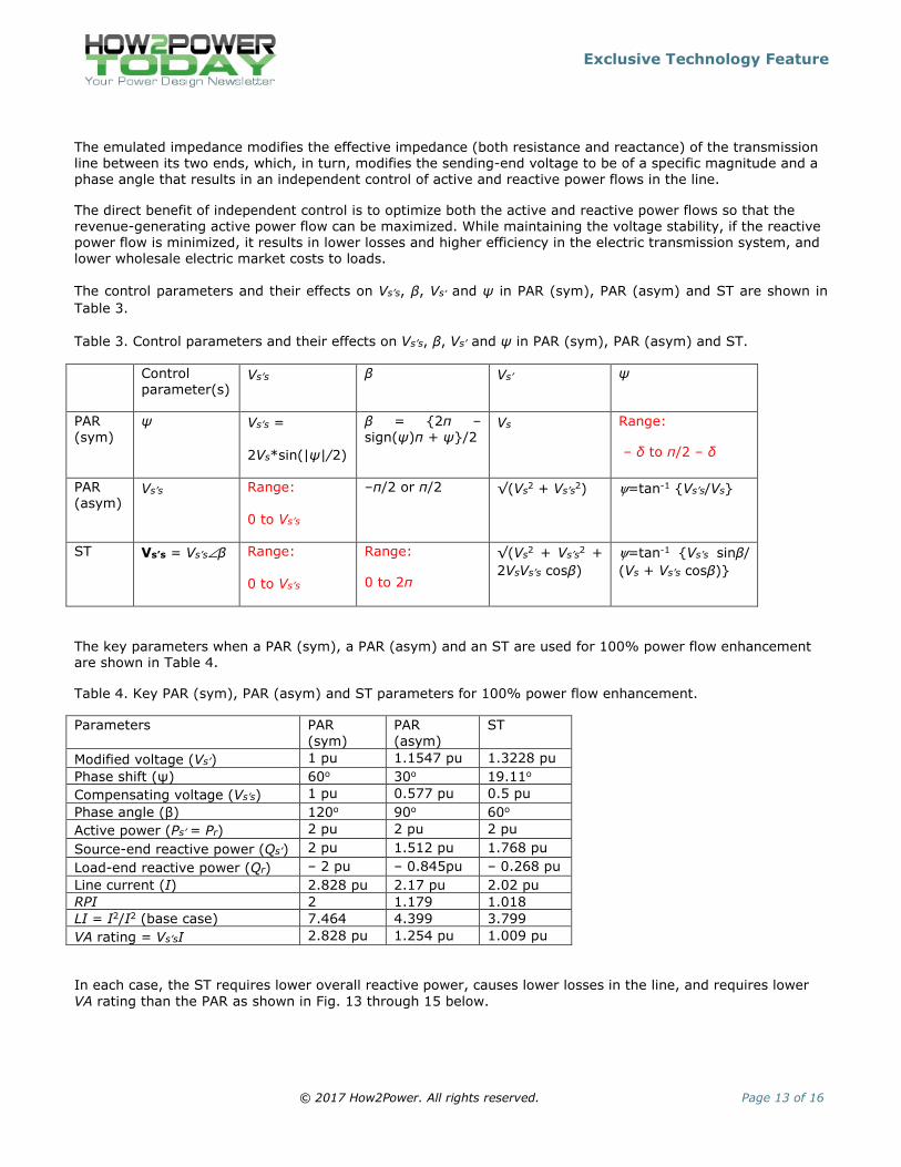
The control parameters and their effects on Vs’s, β, Vs’ and ψ in PAR (sym), PAR (asym) and ST are shown in Table 3.
Table 3. Control parameters and their effects on Vs’s, β, Vs’ and ψ in PAR (sym), PAR (asym) and ST.
Control parameter(s)
Vs’s β Vs’ ψ
PAR (sym)
ψ Vs’s =
2Vs*sin(|ψ|/2)
β = {2π – sign(ψ)π + ψ}/2
Vs Range:
– δ to π/2 – δ
PAR (asym)
Vs’s Range:
0 to Vs’s
–π/2 or π/2 √(Vs2 + Vs’s
2) ψ=tan-1 {Vs’s/Vs}
ST Vs’s = Vs’s∠β Range:
0 to Vs’s
Range:
0 to 2π
√(Vs2 + Vs’s
2 + 2VsVs’s cosβ)
ψ=tan-1 {Vs’s sinβ/ (Vs + Vs’s cosβ)}
The key parameters when a PAR (sym), a PAR (asym) and an ST are used for 100% power flow enhancement are shown in Table 4.
Table 4. Key PAR (sym), PAR (asym) and ST parameters for 100% power flow enhancement.
Parameters PAR (sym)
PAR (asym)
ST
Modified voltage (Vs’) 1 pu 1.1547 pu 1.3228 pu
Phase shift (ψ) 60ο 30ο 19.11ο
Compensating voltage (Vs’s) 1 pu 0.577 pu 0.5 pu
Phase angle (β) 120ο 90ο 60ο
Active power (Ps’ = Pr) 2 pu 2 pu 2 pu
Source-end reactive power (Qs’) 2 pu 1.512 pu 1.768 pu
Load-end reactive power (Qr) – 2 pu – 0.845pu – 0.268 pu
Line current (I) 2.828 pu 2.17 pu 2.02 pu RPI 2 1.179 1.018 LI = I2/I2 (base case) 7.464 4.399 3.799
VA rating = Vs’sI 2.828 pu 1.254 pu 1.009 pu
In each case, the ST requires lower overall reactive power, causes lower losses in the line, and requires lower VA rating than the PAR as shown in Fig. 13 through 15 below.
The limitation of the PAR (sym) is that it is not designed to operate beyond the maximum operating angle (ψmax), represented by the dashed line. Therefore, if the line’s thermal limit is at 2 pu, as it is in this example, it is not possible to achieve the desired power flow using the PAR (sym.)
Conclusion
The implementation of independent active and reactive power flow control using a UPFC is novel. However, the overriding burden of a UPFC is its component obsolescence and high cost. To mitigate these drawbacks, a new idea was proposed, namely the Sen Transformer (ST) that utilizes the best of both—the independent power flow control capability of a UPFC and the established hardware of a PAR to create a viable power flow controller to meet the power flow control needs of the utilities.
While the UPFC promised to bring a new technology that did not exist before, the ST has challenged the established technology of the PAR to change its course and adopt the concept of the ST. Nevertheless, it is a long process to abandon the century-old utility practice of regulating phase angle and adopt regulating impedance for power flow control. In comparison with a PAR, there is no known drawback in an ST. In comparison with a UPFC, a 5:1 reduction in equipment cost and a 10:1 improvement in operational cost for an ST are expected.[6,8]
References
1. “Advanced Solutions in Power Systems: HVDC, FACTS and Artificial Intelligence” by M. Eremia, C-C. Liu and A-A. Edris, IEEE Press and John Wiley & Sons, Chapter 7, 2016.
2. “A unified power flow control concept for flexible AC transmission systems” by L. Gyugyi, Proc. Inst.
Elect. Eng. C, vol. 139, no. 4, Jul. 1992.
3. “AEP unified power flow controller performance” by B. A. Renz, A. Keri, A. S. Mehraban, C. Schauder, E. Stacey, L. Kovalsky, L. Gyugyi, and A-A. Edris, IEEE Trans. on Power Delivery, vol. 14, no. 4, pp. 1374-1381, Oct. 1999.
4. “Comparison of Operational Characteristics between a Sen Transformer and a Phase Angle Regulator” by K. K. Sen and M. L. Sen paper no. 16PESGM0959, IEEE Power & Energy Society General Meeting, Jul. 2016, Boston, USA.
5. “Final Report on the August 14, 2003 Blackout in the United States and Canada: Causes and Recommendations” by U.S.-Canada Power System Outage Task Force, April 2004. Accessed on February 2, 2016.
6. “Introduction to FACTS Controllers: Theory, Modeling, and Applications” by K. K. Sen and M. L. Sen,
IEEE Press and John Wiley & Sons, Chapters 1, 4 and 9, 2009.
7. “Overview Of Voltage Regulation Schemes For Utility And Industrial Applications” by K. K. Sen, How2Power Today, September 2015 issue. Accessed on January 30, 2016.
8. “Comparison of the Sen transformer with the unified power flow controller,” by K. K. Sen and M. L. Sen, IEEE Trans. Power Delivery, vol. 18, no. 3, pp. 1523-1533, Oct. 2003.
Currently the chief technology officer of Sen Engineering Solutions, Kalyan K. Sen
has spent 30 years in academia and industry. Sen who was selected to be a
Westinghouse Fellow Engineer, was a key member of the FACTS development team
at the Westinghouse Science & Technology Center in Pittsburgh. He contributed in
all aspects (conception, simulation, design, and commissioning) of FACTS projects
at Westinghouse. Sen conceived some of the basic concepts in FACTS technology.
He has authored over 25 publications, eight issued patents, one book and four book
chapters in the areas of FACTS and power electronics. He is a licensed Professional
Engineer in the Commonwealth of Pennsylvania.
Sen received BEE, MSEE, and PhD degrees in electrical engineering, from Jadavpur
University, Tuskegee University, and Worcester Polytechnic Institute, respectively.
In addition, he received an MBA from Robert Morris University. A senior member of
IEEE, Sen has served the organization in many positions. Under his leadership, IEEE
Pittsburgh Section and its three chapters (PES, IAS and PELS) received Best Section and Chapter Awards. His
other past positions include Editor of the IEEE Transactions on Power Delivery (2002 – 2007), the Technical
Program Chair of the 2008 PES General Meeting in Pittsburgh, Chapters/Sections Activities Track Chair for the
2008 IEEE Section Congress, Quebec City, Power & Energy Society Region 2 Representative (2010, 2011) and
Member of IEEE Center for Leadership Excellence (CLE) Committee (2013, 2014). He has been serving as an
IEEE Distinguished Lecturer since 2002. In that capacity, he has given presentations on power flow control
technology more than 100 times in 15 countries. He is an inaugural class (2013) graduate of the IEEE CLE
Volunteer Leadership Training (VOLT) program. Sen is the recepient of the IEEE Pittsburgh Section PES
Outstanding Engineer Award (2004) and Outstanding Volunteer Service Award for reviving the local chapters of
PES and IAS from inactivity to world-class performance (2004). He has been serving as the Special Events
Coordinator of the IEEE Pittsburgh Section for the last decade. He is the Region 2&3 Coordinator of Power
Electronics Society. He is a Fulbright Scholar. He is a Distinguished Toastmaster who led District 13 of
Toastmasters International as its Governor to be the 10th-ranking District in the world in 2007-8.
Currently the President of Sen Engineering Solutions, Mey Ling Sen has spent over
15 years in industry. She worked as an Engineering Consultant at Westinghouse and
ABB. She is the co-inventor of the Sen Transformer—a SMART Power Flow Controller
that is based on functional requirements and the most cost-effective power flow
control solution. She is the coauthor of the book titled, Introduction to FACTS Controllers: Theory, Modeling, and Applications, IEEE Press and John Wiley & Sons,
Inc. 2009, which is also published in Chinese.
Sen received BSEE and MEE degrees in electrical engineering, from Worcester
Polytechnic Institute and Rice University, respectively. A member of IEEE, Sen has
served the organization in many positions. Under her leadership, IEEE Pittsburgh
Section PES and IAS Chapters received Best Chapter Awards. She also served as the
Section Treasurer and Co-Chair of Women In Engineering affinity group and Vice
Chair of Pittsburgh Power Electronics Chapter. She led her Club and Area to win the President’s Distinguished