Exercise 2b: Model-based control of the ABB IRB

120

Prof. Marco Hutter∗

Teaching Assistants: Vassilios Tsounis, Jan Carius, Ruben Grandia†

October 31, 2017

Abstract

In this exercise you will learn how to implement control algorithms focusedon model-based control schemes. A MATLAB visualization of the robot armis provided. You will implement controllers which require a motion refer-ence in the joint-space as well as in the operational-space. Finally, you willlearn how to implement a hybrid force and motion operational space con-troller. The partially implemented MATLAB scripts, as well as the visualizer,are available at http://www.rsl.ethz.ch/education-students/lectures/

robotdynamics.html.

Figure 1: The ABB IRW 120 robot arm.

∗original contributors include Michael Blosch, Dario Bellicoso, and Samuel Bachmann†tsounisv@ethz.ch, jan.carius@mavt.ethz.ch, ruben.grandia@mavt.ethz.ch

1

1 Introduction

The robot arm and the dynamic properties are shown in Figure 2. The kinematicand dynamic parameters are given and can be loaded using the provided MATLABscripts. To initialize your workspace, run the init workspace.m script. To startthe visualizer, run the loadviz.m script.

Figure 2: ABB IRB 120 with coordinate systems and joints

2 Model-based control

In this section you will write three controllers which use of the dynamic model ofthe arm to perform motion and force tracking tasks. The template files can befound in the problems/ directory. Each controller comes with its own Simulinkmodel, which is stored under problems/simulink models/. To test each of yourcontrollers, open the corresponding model and start the simulation.

2.1 Joint space control

2

Exercise 2.1

In this exercise you will implement a controller which compensates for the gravita-tional terms. Additionally, the controller should track a desired joint-space configu-ration and provide damping which is proportional to the measured joint velocities.Use the provided Simulink block scheme abb pd g.mdl to test your controller. Whatbehavior would you expect for various initial conditions?

1 function [ tau ] = control pd g( q des, q, q dot )2 % CONTROL PD G Joint space PD controller with gravity compensation.3 %4 % q des −−> a vector Rˆn of desired joint angles.5 % q −−> a vector Rˆn of measured joint angles.6 % q dot −−> a vector in Rˆn of measured joint velocities7

8 % Gains9 % Here the controller response is mainly inertia dependent

10 % so the gains have to be tuned joint−wise11 kp = 0; % TODO12 kd = 0; % TODO13

14 % The control action has a gravity compensation term, as well as a PD15 % feedback action which depends on the current state and the desired16 % configuration.17 tau = zeros(6,1); % TODO18

19 end

2.2 Inverse dynamics control

Exercise 2.2

In this exercise you will implement a controller which uses an operational-spaceinverse dynamics algorithm, i.e. a controller which compensates the entire dynamicsand tracks a desired motion in the operational-space. Use the provided Simulinkmodel stored in abb inv dyn.mdl. To simplify the way the desired orientation isdefined, the Simulink block provides a way to define a set of Euler Angles XYZ,which will be converted to a rotation matrix in the control law script file.

1 function [ tau ] = control inv dyn(I r IE des, eul IE des, q, q dot)2 % CONTROL INV DYN Operational−space inverse dynamics controller ...

with a PD3 % stabilizing feedback term.4 %5 % I r IE des −−> a vector in Rˆ3 which describes the desired ...

position of the6 % end−effector w.r.t. the inertial frame expressed in the ...

inertial frame.7 % eul IE des −−> a set of Euler Angles XYZ which describe the desired8 % end−effector orientation w.r.t. the inertial frame.9 % q −−> a vector in Rˆn of measured joint angles

10 % q dot −−> a vector in Rˆn of measured joint velocities11

12 % Set the joint−space control gains.13 kp = 0; % TODO14 kd = 0; % TODO15

16 % Find jacobians, positions and orientation based on the current17 % measurements.18 I J e = I Je fun solution(q);19 I dJ e = I dJe fun solution(q, q dot);

3

20 T IE = T IE fun solution(q);21 I r Ie = T IE(1:3, 4);22 C IE = T IE(1:3, 1:3);23

24 % Define error orientation using the rotational vector ...parameterization.

25 C IE des = eulAngXyzToRotMat(eul IE des);26 C err = C IE des*C IE';27 orientation error = rotMatToRotVec solution(C err);28

29 % Define the pose error.30 chi err = [I r IE des − I r Ie;31 orientation error];32

33 % PD law, the orientation feedback is a torque around error ...rotation axis

34 % proportional to the error angle.35 tau = zeros(6, 1); % TODO36

37 end

Figure 3: Robot arm cleaning a window

4

2.3 Hybrid force and motion control

Exercise 2.3

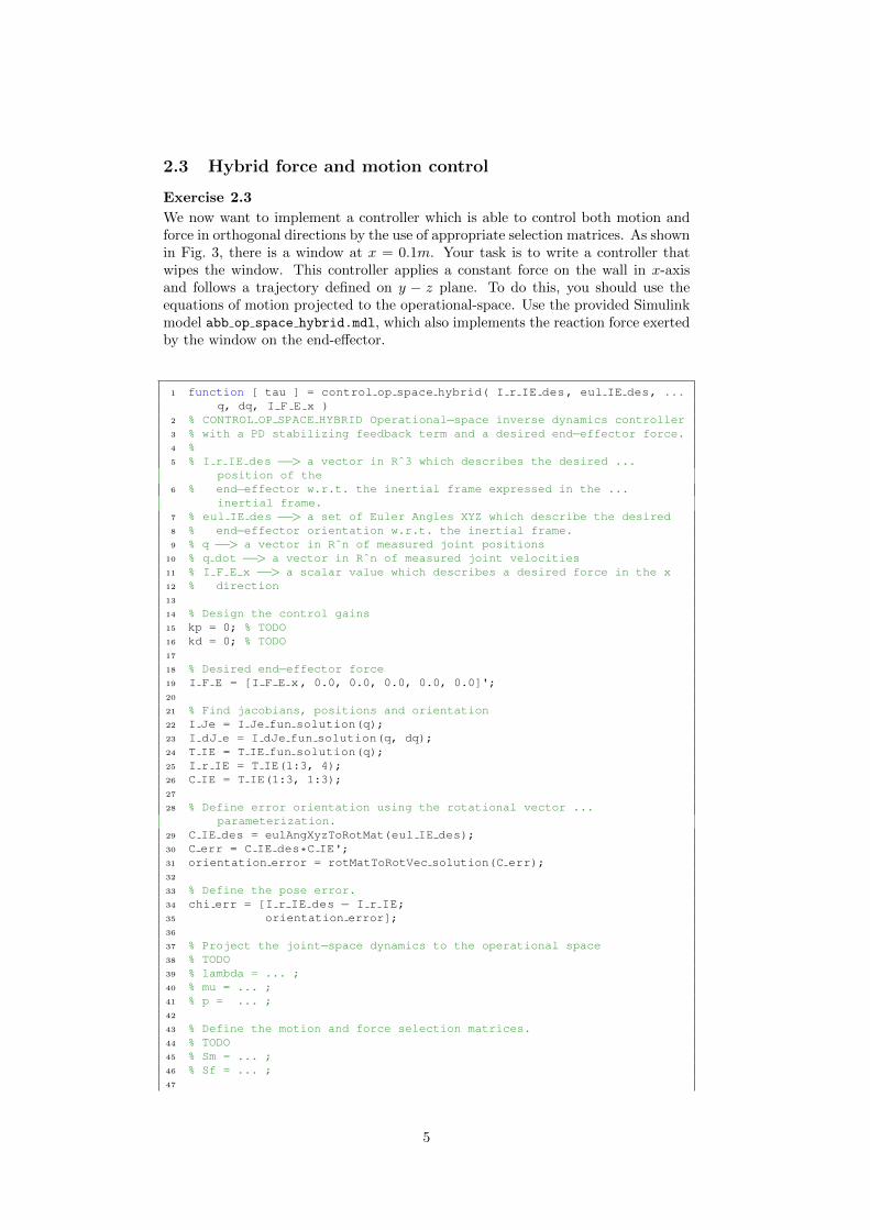
We now want to implement a controller which is able to control both motion andforce in orthogonal directions by the use of appropriate selection matrices. As shownin Fig. 3, there is a window at x = 0.1m. Your task is to write a controller thatwipes the window. This controller applies a constant force on the wall in x-axisand follows a trajectory defined on y − z plane. To do this, you should use theequations of motion projected to the operational-space. Use the provided Simulinkmodel abb op space hybrid.mdl, which also implements the reaction force exertedby the window on the end-effector.

1 function [ tau ] = control op space hybrid( I r IE des, eul IE des, ...q, dq, I F E x )

2 % CONTROL OP SPACE HYBRID Operational−space inverse dynamics controller3 % with a PD stabilizing feedback term and a desired end−effector force.4 %5 % I r IE des −−> a vector in Rˆ3 which describes the desired ...

position of the6 % end−effector w.r.t. the inertial frame expressed in the ...

inertial frame.7 % eul IE des −−> a set of Euler Angles XYZ which describe the desired8 % end−effector orientation w.r.t. the inertial frame.9 % q −−> a vector in Rˆn of measured joint positions

10 % q dot −−> a vector in Rˆn of measured joint velocities11 % I F E x −−> a scalar value which describes a desired force in the x12 % direction13

14 % Design the control gains15 kp = 0; % TODO16 kd = 0; % TODO17

18 % Desired end−effector force19 I F E = [I F E x, 0.0, 0.0, 0.0, 0.0, 0.0]';20

21 % Find jacobians, positions and orientation22 I Je = I Je fun solution(q);23 I dJ e = I dJe fun solution(q, dq);24 T IE = T IE fun solution(q);25 I r IE = T IE(1:3, 4);26 C IE = T IE(1:3, 1:3);27

28 % Define error orientation using the rotational vector ...parameterization.

29 C IE des = eulAngXyzToRotMat(eul IE des);30 C err = C IE des*C IE';31 orientation error = rotMatToRotVec solution(C err);32

33 % Define the pose error.34 chi err = [I r IE des − I r IE;35 orientation error];36

37 % Project the joint−space dynamics to the operational space38 % TODO39 % lambda = ... ;40 % mu = ... ;41 % p = ... ;42

43 % Define the motion and force selection matrices.44 % TODO45 % Sm = ... ;46 % Sf = ... ;47

5

48 % Design a controller which implements the operational−space inverse49 % dynamics and exerts a desired force.50 tau = zeros(6,1); % TODO51

52 end

6