84
Exercises in Occupancy Estimation and Modeling; Donovan and Hines, 2007 Exercise 5: Single-Species, Single-Season Occupancy Models with Survey Covariates Chapter 5 Page 1 2/25/2022

Exercises in Occupancy Estimation and Modeling; Donovan and Hines, 2007
Exercise 5: Single-Species, Single-Season Occupancy Models with Survey Covariates
Chapter 5 Page 1 5/9/2023
Exercises in Occupancy Estimation and Modeling; Donovan and Hines, 2007
TABLE OF CONTENTS
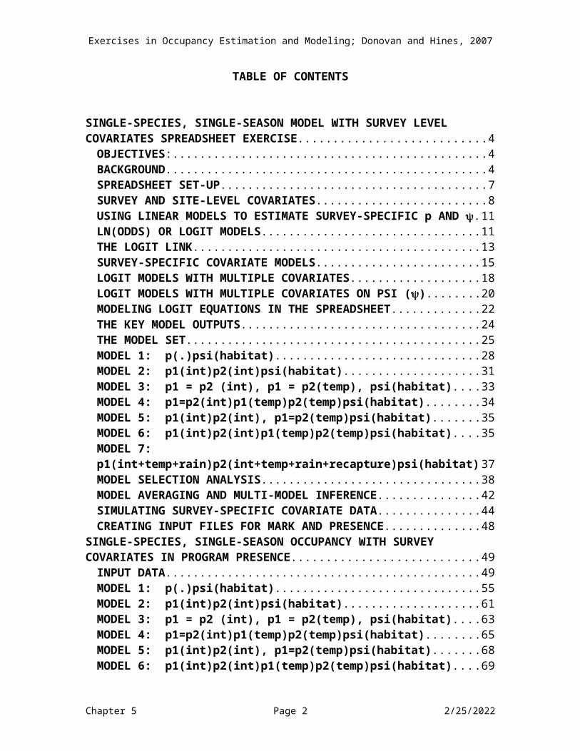
SINGLE-SPECIES, SINGLE-SEASON MODEL WITH SURVEY LEVEL COVARIATES SPREADSHEET EXERCISE............................................4
OBJECTIVES:......................................................................................4BACKGROUND...................................................................................4SPREADSHEET SET-UP....................................................................7SURVEY AND SITE-LEVEL COVARIATES........................................8USING LINEAR MODELS TO ESTIMATE SURVEY-SPECIFIC p AND ........................................................................................................11LN(ODDS) OR LOGIT MODELS......................................................11THE LOGIT LINK..............................................................................13SURVEY-SPECIFIC COVARIATE MODELS.....................................15LOGIT MODELS WITH MULTIPLE COVARIATES..........................18LOGIT MODELS WITH MULTIPLE COVARIATES ON PSI ().......20MODELING LOGIT EQUATIONS IN THE SPREADSHEET..............22THE KEY MODEL OUTPUTS...........................................................24THE MODEL SET..............................................................................25MODEL 1: p(.)psi(habitat)...........................................................28MODEL 2: p1(int)p2(int)psi(habitat).........................................31MODEL 3: p1 = p2 (int), p1 = p2(temp), psi(habitat)............33MODEL 4: p1=p2(int)p1(temp)p2(temp)psi(habitat).............34MODEL 5: p1(int)p2(int), p1=p2(temp)psi(habitat)...............35MODEL 6: p1(int)p2(int)p1(temp)p2(temp)psi(habitat)........35MODEL 7: p1(int+temp+rain)p2(int+temp+rain+recapture)psi(habitat)..........................................................................................................37MODEL SELECTION ANALYSIS......................................................38MODEL AVERAGING AND MULTI-MODEL INFERENCE...............42SIMULATING SURVEY-SPECIFIC COVARIATE DATA...................44CREATING INPUT FILES FOR MARK AND PRESENCE.................48
SINGLE-SPECIES, SINGLE-SEASON OCCUPANCY WITH SURVEY COVARIATES IN PROGRAM PRESENCE...........................................49
INPUT DATA....................................................................................49MODEL 1: p(.)psi(habitat)...........................................................55MODEL 2: p1(int)p2(int)psi(habitat).........................................61MODEL 3: p1 = p2 (int), p1 = p2(temp), psi(habitat)............63MODEL 4: p1=p2(int)p1(temp)p2(temp)psi(habitat).............65MODEL 5: p1(int)p2(int), p1=p2(temp)psi(habitat)...............68MODEL 6: p1(int)p2(int)p1(temp)p2(temp)psi(habitat)........69MODEL 7: p1(int+temp+rain)p2(int+temp+rain+recapture)psi(habitat)..........................................................................................................71SUMMARY........................................................................................74
Chapter 5 Page 2 5/9/2023

Exercises in Occupancy Estimation and Modeling; Donovan and Hines, 2007
Chapter 5 Page 3 5/9/2023

Exercises in Occupancy Estimation and Modeling; Donovan and Hines, 2007
SINGLE-SPECIES, SINGLE-SEASON MODEL WITH SURVEY LEVEL COVARIATES SPREADSHEET EXERCISE
OBJECTIVES: To learn and understand how survey-level covariates are
evaluated in a basic occupancy model. To understand and apply “trap response” covariates. To use Solver to find the maximum likelihood estimates for the
probability of detection and the probability of site occupancy, given a set of covariates.
To use model selection approaches to compare and rank models. To compute model averaged estimates of p1, p2, and . To learn how to simulate occupancy data with survey-level
covariates.
BACKGROUNDNow that you have a handle on the general occupancy models with site-level covariates, we can add an additional twist: survey-specific covariates. The information for this exercise roughly follows the materials presented in chapter 4 in the book, Occupancy Modeling and Estimation. Click on the worksheet labeled “Survey Covariates.” In this exercise, we’ll review many of the covariate concepts previously covered – simply to reinforce the ideas because almost all “real” analyses involve covariates to some degree.
Let’s step back for a second, and answer the question, “what exactly is meant by a “survey-specific covariate” effect?” Well, remember the parameters of the “general” occupancy model we ran in Exercise 3: p1, p2, p3, and . The only raw data we had to run a model was the encounter history frequencies. We basically found the combination of parameter estimates that maximized the multinomial log likelihood. But with covariate analyses, in addition to the encounter histories, a lot
Chapter 5 Page 4 5/9/2023

Exercises in Occupancy Estimation and Modeling; Donovan and Hines, 2007
of other data is collected to describe the site and survey conditions. In exercise 4, we analyzed psi as a function of the physical and biological characteristics of the site (patch size, patch size2, habitat), and called these “site-level covariates.” In this exercise, we will evaluate one site-level covariate that affects psi (habitat), but our focus will be on analyzing survey-specific covariates that are thought to affect detection probability. For example, you might collect data on the date the site was sampled, the time the site was sampled, the weather conditions of the sampling period. If you sampled the same site on three different days, and think that “temperature” could affect detection probability, then you could add the following constraints to p:- p1 is a function of the temperature in which sample 1 occurred.- p2 is a function of the temperature in which sample 2 occurred. - p3 is a function of the temperature in which sample 3 occurred. In this case, the date is called a “survey” covariate because detection on a particular survey is a function of the date in which the site was surveyed.
In this spreadsheet, we’ll assume that you design a study in which 200 sites are studied, and each site is surveyed two times, with surveys occurring on different days. This is a realistic scenario. Here, the replicate surveys are done over time. Thus, the conditions in which the two surveys occur can be dramatically different, and the covariates associated with each survey are important.
In this exercise, there is a single occupancy covariate, habitat. There are three habitat types, and thus two covariates are estimated to determine the effect of habitat on occupancy probability. The detection covariates we’ll explore are the temperature in which the site was surveyed, whether the site was surveyed in the rain, and a
Chapter 5 Page 5 5/9/2023
Exercises in Occupancy Estimation and Modeling; Donovan and Hines, 2007
“trap response” covariate. Temperature is an example of continuous covariate, while rain is a categorical covariate.
The “trap response” is also a categorical survey covariate. If you have studied closed-capture models, the “trap response” concept will come easily to you. To explain this response, it’s first useful to recall the underlying assumptions of the general, single-season occupancy model:
1) The system is demographically closed to changes in the occupancy status of site during the sampling period. At the species level, this means that a species cannot colonize/immigrate to a site, or go locally extinct/emigrate from that site during the course of the study.
2) Species are not falsely detected. 3) Detection at a site is independent of detection at other sites.
This means that your sites should be far enough apart to be biologically independent.
Even if the first two assumptions are met, there may be cases when the third assumption is violated. Although each site is supposed to be independent of other sites, what about independence of samples within a site? If you survey the same site over time, or the same site over space, there is likely to be some dependence among your sampling efforts. While this in and of itself is not a violation of occupancy modeling, if the dependence is strong, you may end up with encounter histories that reflect a “trap response.”
An example might make this clear. Suppose we survey the same site in two successive days. If you detect the species on day 1, and the species or site is “trap happy”, then you may be more likely to detect the species again on day 2, increasing the number of 11 histories. In contrast, if you detect the species on day 1 and the species or site is
Chapter 5 Page 6 5/9/2023

Exercises in Occupancy Estimation and Modeling; Donovan and Hines, 2007
“trap shy”, then you may be more likely to miss the species on day 2, increasing the number of 10 histories. So the outcome of the second survey is tied to the outcome of the first survey in some way. In this exercise, we’ll explore this response in detail, as well as other survey-specific covariates that affect detection probability.
As we did in the previous exercise, we’ll run several different, competing models, and then we’ll use model selection procedures to compare different models. Finally, we’ll compute the model-averaged estimates of p1, p2, and p3 for all sites. Let’s get started.
SPREADSHEET SET-UPThis spreadsheet is set up similarly to that in the previous one. As in the previous exercise, there are only 2 sampling sessions for each site.
171819202122
A B C D EOriginal Site Survey 1 Survey 2 History
01 1 0 1 0101 2 0 1 0111 3 1 1 1111 4 1 1 1111 5 1 1 11
For now, note that the sites are given in column B, the results of Survey 1 are given in column C, the results of Survey 2 are given in column D, and the history associated with each site is given in Column E. Since there are only 2 capture sessions in this example, there are only 22 = 4 possible histories: 11, 10, 00, and 01. These histories are summed across the sites in cells F4:I4 with a COUNTIF function. (Note: we won't actually analyze these summed histories...they're just there to summarize the data.)
Chapter 5 Page 7 5/9/2023

Exercises in Occupancy Estimation and Modeling; Donovan and Hines, 2007
2
3
4
F G H I J
11 10 01 00 Total107 14 27 52 200
Summarized Inputs
Note that for this spreadsheet example, there are 200 sites (cell J4). This will allow Solver to work a bit more quickly.
*******************************************************************NOTE: BEFORE GOING ANY FURTHER, MAKE SURE THAT THE HISTORIES IN COLUMN E MATCH THOSE IN COLUMN A. IF THEY DON’T MATCH, COPY CELLS A18:A217 AND PASTE THEM INTO CELLS E18:E217. *******************************************************************
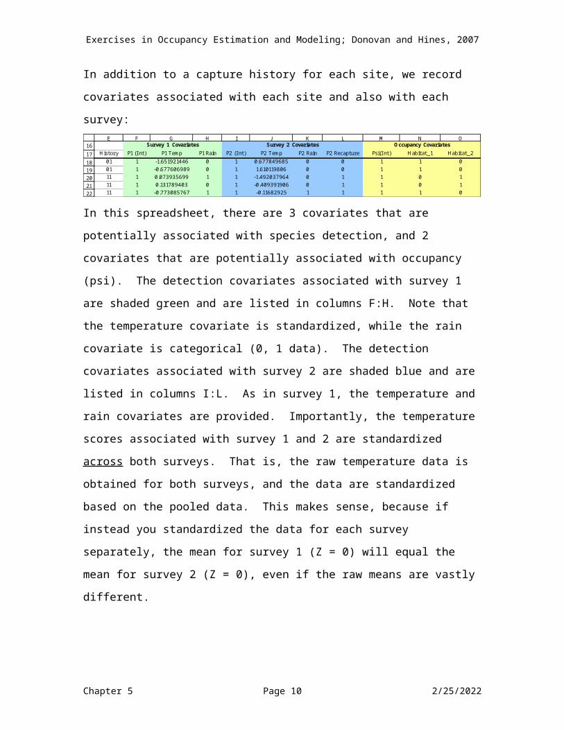
SURVEY-SPECIFIC AND SITE-LEVEL COVARIATESIn addition to a capture history for each site, we record covariates associated with each site and also with each survey:
16171819202122
E F G H I J K L M N O
History P1 (I nt) P1 Temp P1 Rain P2 (I nt) P2 Temp P2 Rain P2 Recapture Psi(I nt) Habitat_1 Habitat_201 1 -1.651921446 0 1 0.677849685 0 0 1 1 001 1 -0.677606989 0 1 1.610119806 0 0 1 1 011 1 0.073935699 1 1 -1.492037964 0 1 1 0 111 1 0.131789403 0 1 -0.409391906 0 1 1 0 111 1 -0.773085767 1 1 -0.11682925 1 1 1 1 0
Survey 1 Covariates Survey 2 Covariates Occupancy Covariates
In this spreadsheet, there are 3 covariates that are potentially associated with species detection, and 2 covariates that are potentially associated with occupancy (psi). The detection covariates associated with survey 1 are shaded green and are listed in columns F:H. Note that the temperature covariate is standardized, while the rain covariate is categorical (0, 1 data). The detection covariates associated with survey 2 are shaded blue and are listed in columns I:L. As in survey 1, the temperature and rain covariates are provided. Importantly, the temperature scores associated with survey 1 and 2 are standardized across both surveys. That is, the raw temperature data is obtained for both surveys, and the data are standardized based
Chapter 5 Page 8 5/9/2023

Exercises in Occupancy Estimation and Modeling; Donovan and Hines, 2007
on the pooled data. This makes sense, because if instead you standardized the data for each survey separately, the mean for survey 1 (Z = 0) will equal the mean for survey 2 (Z = 0), even if the raw means are vastly different.
Column L provides the “trap” response covariate, and is obtained from the histories themselves (rather than the conditions of the site or survey). This covariate applies to p2 only. For example, the first two histories are 01 – the species was not detected on the first survey, so it cannot have a “trap response” because it was not “captured” in the first survey. Thus, cells L18:L19 are 0 for those sites.
16171819202122
E L
History Recapture01 001 011 111 111 1
Survey 2 Covariates
Sites 3-5 each had a 11 history, indicating the species was detected on the first and second surveys. Because of the first detection, cells L20:22 are coded 1, indicating that there is a potential trap response for survey two. If a site had a 10 history, it would also receive a “1” for the recapture covariate, indicating there is a potential trap response for survey 2.
The two occupancy covariates are given in columns N and O, and are shaded yellow (in addition to the psi intercept). These two site-level covariates code for habitat type, a categorical variable. There were three habitats surveyed, and the 0 and 1 coding for Habitat1 and Habitat2 reveals the habitat type associated with each site. If the site was surveyed in habitat 1, then Habitat1 = 1. If Habitat1 = 0, then the site was not characterized as habitat 1. If the site was surveyed in
Chapter 5 Page 9 5/9/2023
Exercises in Occupancy Estimation and Modeling; Donovan and Hines, 2007
habitat type 2, then Habitat2 = 1. If Habitat2 = 0, the site was not located in habitat type 2. By this coding, if Habitat1 = 0 and Habitat2 = 0, the site is located in habitat 3. Because habitat 3 is coded as 0 0, it is called the “reference habitat” and the other habitat types are compared to it. You can make the reference habitat any type you want (1, 2, or 3) by altering your coding system. Using this coding system, sites 1 and 2 were in habitat 1, sites 3 and 4 were in habitat 2, and sites 9 and 10 were in habitat 3.
USING LINEAR MODELS TO ESTIMATE SURVEY-SPECIFIC p AND
OK, now given each site's survey and site covariate values, we need to determine what p1, p2, and are for each site. Let’s focus on only temperature to begin with, considering only survey 1 for now. Much of the following discussion will be a review, but it won’t hurt to read it again. Let’s assume that as the standardized Z score for temperature increases or decreases, the probability of detection increases or decreases in a predictable fashion. We could use a regression model to do this:
p1 = B0 + B1 * covariate, or in our case…p1 = B0 + B1 * standardized temperature.
OK, if you’ve taken an introductory stats course you’ll notice that this is the equation of a line (y = mx+b, or y = B0 + B1x) and by knowing B0
and B1, as well as a site’s Z score for temperature, you can estimate p1 with linear regression approaches. If B1 is positive, the relationship is positive, where sites with high Z scores (i.e., those sites sampled in warmer temperatures) will have a higher detection probability, and if B1 is negative, the relationship is a negative relationship where sites with high Z scores will have a lower detection probability.
Chapter 5 Page 10 5/9/2023

Exercises in Occupancy Estimation and Modeling; Donovan and Hines, 2007
LN(ODDS) OR LOGIT MODELSBut, hang on! P1 is a probability, and is bounded between 0 and 1. We can’t do a regression analysis for this model because the analysis requires that the response variable (p1) be unbounded. What now? The way around this problem involves converting the probability, p1 to odds, and then taking the natural log of the odds, and then modeling the log odds (or logit) of p1 instead of p1 and then back-transforming the logit of p1 to get p1. Hmmmm, let’s try that more slowly. You’re all familiar with odds (e.g., “what are the odds that the Chicago Cubs will win the World Series this year?”). Suppose the Cubs play a 10-game season and we record the number of possible wins and losses. The odds are computed as the ratio of wins:losses, or wins/losses. For example, if for every 10 games played there are 9 wins and 1 loss, the odds of winning are 9:1 = 9/1 = 9. The relationship between probability and odds is expressed with the following equation:
probability = odds / (1+odds).
Thus, if the odds of winning is 9:1, the probability of winning is 9/10 = 0.9.
wins losses odds probability ln (odds)0 10 0.000 0 #NUM!1 9 0.111 0.1 -2.197222 8 0.250 0.2 -1.386293 7 0.429 0.3 -0.84734 6 0.667 0.4 -0.405475 5 1.000 0.5 06 4 1.500 0.6 0.405477 3 2.333 0.7 0.84738 2 4.000 0.8 1.386299 1 9.000 0.9 2.1972210 0 #DI V/ 0! #DI V/ 0! #DI V/ 0!
Chapter 5 Page 11 5/9/2023

Exercises in Occupancy Estimation and Modeling; Donovan and Hines, 2007
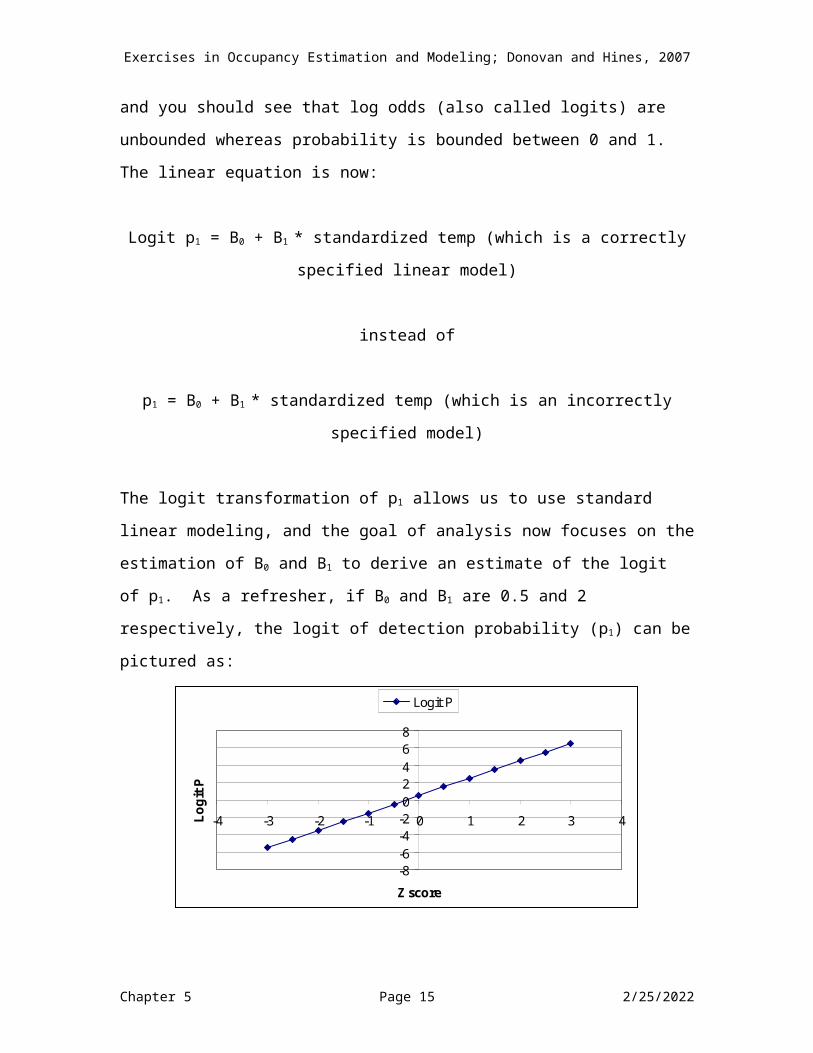
Take a good look at the table above. Notice anything special about “odds”? They range from 0 to positive infinity (in theory). So by using odds instead of probability in our linear equation, we take care of the probability bounding issue on the positive side (unlike probability, odds are not bounded to be less than 1). However, we still need to deal with the negative “boundedness.” How? We take the natural log of the odds, or ln (odds). Look at the far right column in the table above and you should see that log odds (also called logits) are unbounded whereas probability is bounded between 0 and 1.The linear equation is now:
Logit p1 = B0 + B1 * standardized temp (which is a correctly specified linear model)
instead of
p1 = B0 + B1 * standardized temp (which is an incorrectly specified model)
The logit transformation of p1 allows us to use standard linear modeling, and the goal of analysis now focuses on the estimation of B0 and B1 to derive an estimate of the logit of p1. As a refresher, if B0 and B1 are 0.5 and 2 respectively, the logit of detection probability (p1) can be pictured as:
Chapter 5 Page 12 5/9/2023

Exercises in Occupancy Estimation and Modeling; Donovan and Hines, 2007
-8-6-4-202468
-4 -3 -2 -1 0 1 2 3 4
Z score
Logi
t P
Logit P
THE LOGIT LINKBut logit p1 doesn’t intuitively make sense because we’re really interested in understanding how detection probability is associated with survey temperature. So how do you transform the logit back to a probability? You take the anti-logit, which has the form:
p1 = Exp(B0 + B1* standardized temp) / (1+ Exp(B0 + B1*standardized temp))
which back transforms the log and odds computations, or more generally
Exp(linear equation)/(1+exp(linear equation)
This gets you back to the probability, p1, and the equation for converting logits to probabilities is called the logit link. In MARK and PRESENCE, the logit link is the default link when covariates are used in a model. Below is a graph of the logit as a function of standardized date (left hand scale, diamonds), where B0 = 0.5 and B1 = 2. A second series graphs the back-transformed p1 as a function of standardized temperature (right hand scale, squares). Note the linear relationship
Chapter 5 Page 13 5/9/2023

Exercises in Occupancy Estimation and Modeling; Donovan and Hines, 2007
between logit and standardized temp, whereas the relationship between p and standardized temp is an s-shaped (logistic) function.
-8-6-4-202468
-4 -3 -2 -1 0 1 2 3 4
Z score
Logi
t P
0
0.2
0.4
0.6
0.8
1
P
Dete
ctio
n Pr
obab
ility
Logit P P
How does this apply to our occupancy model? In this case, the anti-logit gives us p1, and it does so for each site because we replace words “standardized temperature” in the equation above with the Z temp for survey 1 at each specific site. An example might make this clearer. If B0 = 0.5 and B1 = 2, a site with a standardized survey temp of Z = +0.75 will have p1 =Exp(0.5 + 2*0.75) / (1+ Exp(0.5 + 2*0.75))=0.8808, whereas a site with a standardized temp of Z = -0.75 would have p1 =Exp(0.5 + 2*-0.75) / (1+ Exp(0.5 + 2*-0.75))=0.26894. That’s quite a difference in p1 between the two sites! In this case, the site that was surveyed in colder temperatures (Z = -0.75) had a much lower detection probability (p1 = 0.26894) than a site that was surveyed in warmer temperatures (p1 = 0.8808).
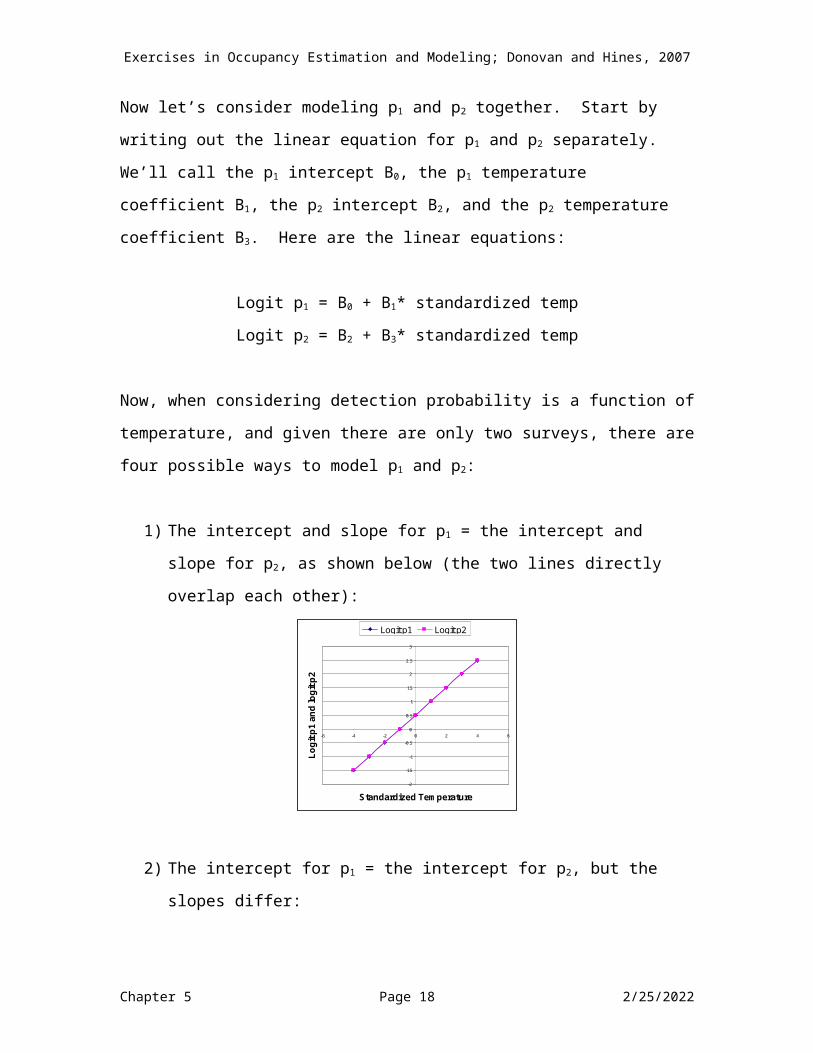
SURVEY-SPECIFIC COVARIATE MODELSNow let’s consider modeling p1 and p2 together. Start by writing out the linear equation for p1 and p2 separately. We’ll call the p1 intercept B0, the p1 temperature coefficient B1, the p2 intercept B2, and the p2 temperature coefficient B3. Here are the linear equations:
Chapter 5 Page 14 5/9/2023
Exercises in Occupancy Estimation and Modeling; Donovan and Hines, 2007
Logit p1 = B0 + B1* standardized tempLogit p2 = B2 + B3* standardized temp
Now, when considering detection probability is a function of temperature, and given there are only two surveys, there are four possible ways to model p1 and p2:
1) The intercept and slope for p1 = the intercept and slope for p2, as shown below (the two lines directly overlap each other):
-2
-1.5
-1
-0.5
0
0.5
1
1.5
2
2.5
3
-6 -4 -2 0 2 4 6
Standardized Temperature
Logi
t p1
and
logi
t p2
Logit p1 Logit p2
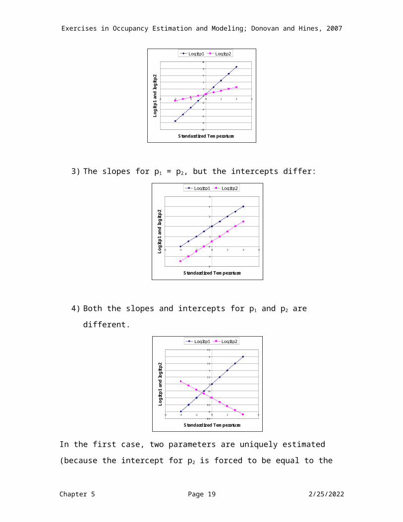
2) The intercept for p1 = the intercept for p2, but the slopes differ:
-10
-8
-6
-4
-2
0
2
4
6
8
10
-6 -4 -2 0 2 4 6
Standardized Temperature
Logi
t p1
and
logi
t p2
Logit p1 Logit p2
3) The slopes for p1 = p2, but the intercepts differ:
Chapter 5 Page 15 5/9/2023

Exercises in Occupancy Estimation and Modeling; Donovan and Hines, 2007
-2
-1
0
1
2
3
4
5
-6 -4 -2 0 2 4 6
Standardized Temperature
Logi
t p1
and
logi
t p2
Logit p1 Logit p2
4) Both the slopes and intercepts for p1 and p2 are different.
-0.5
0
0.5
1
1.5
2
2.5
3
3.5
4
4.5
-6 -4 -2 0 2 4 6
Standardized Temperature
Logi
t p1
and
logi
t p2
Logit p1 Logit p2
In the first case, two parameters are uniquely estimated (because the intercept for p2 is forced to be equal to the intercept for p1, and because the slope for p2 is forced to be equal to the slope for p1). In the second and third case, three parameters are uniquely estimated, and in the fourth case, four parameters are uniquely estimated. With survey-specific data, it is often the case that you will explore all four options to determine which model best describes your observed field data.
LOGIT MODELS WITH MULTIPLE COVARIATES Now, what if p2 was a function of 3 covariates (temperature, rain, and recapture)? Well, we simply expand our linear model to include the additional effects (label the betas what you’d like):
Chapter 5 Page 16 5/9/2023

Exercises in Occupancy Estimation and Modeling; Donovan and Hines, 2007
Logit p2 = B0 + B1 * temp+ B2 * rain + B3 * recapture.
If p1 and are assumed to be intercept models (no covariates), this model would be called p1(.)p2(temp + rain + recapture)psi(.), and the focus of the analysis would be on estimating B0 (the intercept for p2), B1 (the coefficient for temp), B2 (the coefficient for rain) and B3 (the coefficient for recapture) to derive p2 for each site, as well as the intercept for p1 and . This is called an additive model for p2, because the effects are simply added together and each piece of additional information (temp, rain, recapture) simply builds on the other effects. Let’s look at the first 3 sites and assume that B0 = 0.5, B1 = -2, B2 = 0.1, and B3 = 0.5.
1617181920
E I J K L
History P2 (I nt) P2 Temp P2 Rain P2 Recapture01 1 0.677849685 0 001 1 1.610119806 0 011 1 -1.492037964 0 1
Survey 2 Covariates
Given these betas, we can predict logit p2 for each site, and then back-transform the logit with the link function:
Site 1 logit p2 = 0.5*1 + -2*0.6778 + 0.1*0 + 0.5*0 = -0.8556Site 1 p2 = exp(-0.8556)/(1+exp(-0.8556)) =0.298.
Site 2 logit p2 = 0.5*1 + -2*01.61 + 0.1*0 + 0.5*0 = -2.72Site 2 p2 = exp(-2.72)/(1+exp(-2.72)) = 0.0618.
Site 3 logit p2 = 0.5*1 + -2*-1.49 + 0.1*0 + 0.5*1 = 3.98Site 3 p2 = exp(3.98)/(1+exp(3.98)) = 0.982.
Thus, each site has a unique detection probability, p2, associated with it, depending on what the site’s covariate values are. In this example,
Chapter 5 Page 17 5/9/2023
Exercises in Occupancy Estimation and Modeling; Donovan and Hines, 2007
the betas indicate that p2 decreases as temperature increases, increases slightly with rain, and increases if the species was also detected in survey 1 (a trap-happy response). It’s very instructive to study these results: site 1 has a poor detection probability during survey 2 because it was surveyed in warm temperatures, with no rain, and survey 1 also had 0 detections. The beta for temp is -2.0, a strong negative effect, indicating that sites surveyed in cold temperatures (low Z scores) have a higher detection probability. Rain had a beta = +0.1, which is a small effect size, indicating that detection probability increases slightly if survey 2 was conducted in the rain. But since the survey was not conducted in the rain, it does not receive that additional increase in detection probability. Recapture also has a positive effect (beta = 0.5), indicating that if the species was detected on survey 1, the chance of detecting it on survey 2 increases. So, site 1 had a low detection probability overall because it had the wrong combination for all three covariate values. Site 2 also had a combination of covariates that led to a low p2 (in this case, even lower than site 1), primarily because it was surveyed in very warm temperatures. Now let’s look at site 3, which had a high detection probability. This site was surveyed in cold temperatures, which increased its detection probability. It didn’t rain during the survey, but because the species was detected in survey 1, the recapture score was 1, which further increased p2.
LOGIT MODELS WITH MULTIPLE COVARIATES ON PSI ()The same rationale applies to adding covariates to , the probability that a site is occupied. But note that cannot vary as a function of survey period because, a priori, the site is assumed to be closed to changes in occupancy pattern over time. In this spreadsheet exercise, we will model psi as a function of habitat only. If psi is a function of habitat, the linear equation becomes:
Chapter 5 Page 18 5/9/2023
Exercises in Occupancy Estimation and Modeling; Donovan and Hines, 2007
Logit = B000 + B8*habitat1 + B9*habitat2, where the beta subscripts correspond to those in the spreadsheet:
9
10
111213
M N O
B000 Habitat 1 Habitat 2Cov 8 Cov 10 Cov 11
1 1 11.000000 2.000000 0.100000
Occupancy
And we can back-transform the logit to a probability with the logit link:psi = exp(B000 + B8*habitat1 + B9*habitat2)/(1+exp(B000 + B8*habitat1 + B9*habitat2)). Let’s assume that the intercept (call it B00) = 1.00, B5
= 2.00, and B6 = 0.10 (cells M13:O13). Now let’s look at the first three sites and predict what psi is for each site:
1617181920
M N O
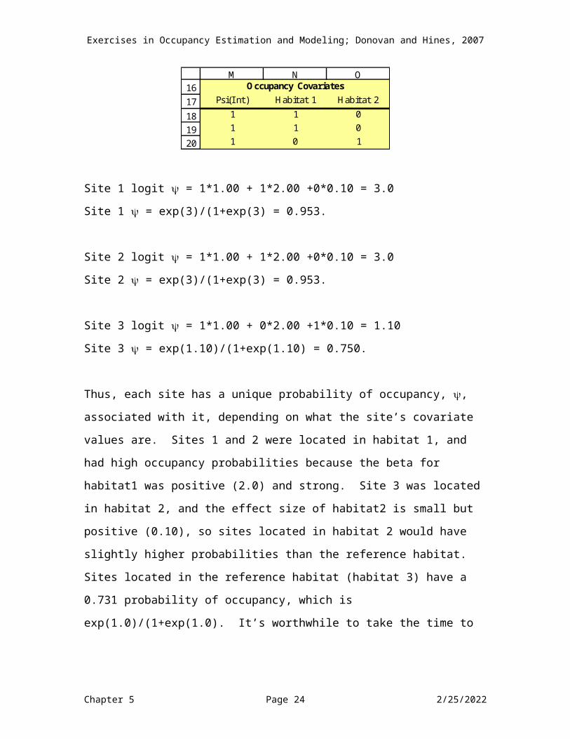
Psi(I nt) Habitat 1 Habitat 21 1 01 1 01 0 1
Occupancy Covariates
Site 1 logit = 1*1.00 + 1*2.00 +0*0.10 = 3.0Site 1 = exp(3)/(1+exp(3) = 0.953.
Site 2 logit = 1*1.00 + 1*2.00 +0*0.10 = 3.0Site 2 = exp(3)/(1+exp(3) = 0.953.
Site 3 logit = 1*1.00 + 0*2.00 +1*0.10 = 1.10Site 3 = exp(1.10)/(1+exp(1.10) = 0.750.
Chapter 5 Page 19 5/9/2023
Exercises in Occupancy Estimation and Modeling; Donovan and Hines, 2007
Thus, each site has a unique probability of occupancy, , associated with it, depending on what the site’s covariate values are. Sites 1 and 2 were located in habitat 1, and had high occupancy probabilities because the beta for habitat1 was positive (2.0) and strong. Site 3 was located in habitat 2, and the effect size of habitat2 is small but positive (0.10), so sites located in habitat 2 would have slightly higher probabilities than the reference habitat. Sites located in the reference habitat (habitat 3) have a 0.731 probability of occupancy, which is exp(1.0)/(1+exp(1.0). It’s worthwhile to take the time to understand exactly what the betas mean, and assess the magnitude of their effects.
MODELING LOGIT EQUATIONS IN THE SPREADSHEETNow, let’s see how all of this is applied within the spreadsheet environment. First, let’s get oriented to the section of the spreadsheet where you specify the model. Cells F10:O10 list the parameters. There are three p1 parameters (p1 intercept, temp and rain), four p2 parameters (p2 intercept, temp, rain, and recapture), and three psi parameters ( intercept, habitat1, and habitat2).
9
10
111213
E F G H I J K L M N O
B0 Temp Rain B00 Temp Rain Recapture B000 Habitat 1 Habitat 2Parameter Cov 1 Cov 2 Cov 3 Cov 4 Cov 5 Cov 6 Cov 7 Cov 8 Cov 10 Cov 11Estimate? 1 0 0 1 0 0 0 1 0 0Beta 0.000000 0.000000 0.000000 0.000000 0 0.000000 0.000000
Survey 1 Survey 2 Occupancy
In cells F12:O12, you enter a 1 under the corresponding parameter to indicate that you want to estimate that parameter for a given model, and a 0 to indicate that you won’t be estimating that parameter for a given model. Cell M12 MUST be equal to 1 because you have to estimate the intercept for psi, and either cell F12 or cell I12 must be 1 because you must estimate at least one intercept for detection. Notice that when a 0 is entered, the cell takes on a pink shade (the cells are conditionally formatted). Underneath the “Estimate?” row is the Beta row.
Chapter 5 Page 20 5/9/2023

Exercises in Occupancy Estimation and Modeling; Donovan and Hines, 2007
9
10
111213
E F G H I J K L M N O
B0 Temp Rain B00 Temp Rain Recapture B000 Habitat 1 Habitat 2Parameter Cov 1 Cov 2 Cov 3 Cov 4 Cov 5 Cov 6 Cov 7 Cov 8 Cov 10 Cov 11Estimate? 1 0 0 1 0 0 0 1 0 0Beta 0.000000 0.000000 0.000000 0.000000 0 0.000000 0.000000
Survey 1 Survey 2 Occupancy
Solver will work on finding the values in the empty cells, so you can leave them blank, except that you must enter a 0 in those cells for any parameter that is not being estimated. (Thus, if a certain parameter is not being estimated, the Estimate? cell will be pink, and you must enter a 0 in its corresponding beta beneath it). This is necessary to count the number of parameters estimated correctly, and to ensure that logits for p1, p2, and are computed correctly. So, the model shown above is set up to estimate the intercept for p1, the intercept for p2, and the intercept for psi. In other words, the model depicted is p1(.)p2(.)psi(.), or more generally psi(.)p(t). By forcing the betas for all covariate effects to be 0, the covariates do not enter the linear equation for estimating the logit of p1, the logit of p2, or the logit of psi. In this example, Solver will find values for cells F13, I13, and M13 that maximize the multinomial log likelihood.
If instead you wished to run model p(.)psi(.), and force the intercept for p2 to be equal to the intercept for p1, you would set up the spreadsheet as follows:
9
10
111213
E F G H I J K L
B0 Temp Rain B00 Temp Rain RecaptureParameter Cov 1 Cov 2 Cov 3 Cov 4 Cov 5 Cov 6 Cov 7Estimate? 1 0 0 0 0 0 0Beta 0 0 =F13 0 0 0
Survey 1 Survey 2
Now let’s look at how the spreadsheet computes p1, p2, and for each site, depending on the site’s covariate values. These probabilities are computed in columns P, Q, and R.
1617
P Q R
p1 p2 Parameter Estimates
Chapter 5 Page 21 5/9/2023

Exercises in Occupancy Estimation and Modeling; Donovan and Hines, 2007
Cell P18 (p1 for site 1) has the equation =EXP(SUMPRODUCT($F$13:$H$13,F18:H18))/(1+EXP(SUMPRODUCT($F$13:$H$13,F18:H18))). This equation uses Excel’s SUMPRODUCT function again to compute the logit of p1, and then back-transforms the logit to a probability within the same function. In other words, Logit p1 = B0 + B2*temp + B3*rainp1 = exp(B0 + B2*temp + B3*rain)/(1+ exp(B0 + B2*temp + B3*rain)).
Similarly, p2 for site 1 is computed in cell Q18 with the equation =EXP(SUMPRODUCT($I$13:$L$13,I18:L18))/(1+EXP(SUMPRODUCT($I$13:$L$13,I18:L18))) and for site 1 is computed in cell R18 with the equation =EXP(SUMPRODUCT($M$13:$O$13,M18:O18))/(1+EXP(SUMPRODUCT($M$13:$O$13,M18:O18))). Click on one of these cells, then click on the equation in the formula bar and you’ll see the equation “light up”, showing the cells used in the formula.
These three equations are copied down columns to generate the p1, p2, and for the remaining sites. Make sense? If it doesn’t, spend a bit of time thinking about the linear equations and their back transformations to probabilities.
THE KEY MODEL OUTPUTSGiven a model’s beta estimates, and hence estimates of p1, p2, and for each site, we can now compute the model’s LogeL. In columns S:V, equations are entered to compute the probability of observing 11, 10, 01, and 00 histories for each site. The probability of observing the encounter history that was observed in the field is computed in column W with an HLOOKUP function. Click on these cells and examine the
Chapter 5 Page 22 5/9/2023

Exercises in Occupancy Estimation and Modeling; Donovan and Hines, 2007
formulae that underlie them….this should be a review to you by now. Here are the formulae:
16171819
S T U V W XObserved
11 10 01 00 Prob. History Ln L =R18*P18*Q18 =R18*P18*(1-Q18) =R18*(1-P18)*Q18 =R18*(1-P18)*(1-Q18)+(1-R18) =HLOOKUP(E18,$S$17:$V$217,B18+1,FALSE) =LN(W18)=R19*P19*Q19 =R19*P19*(1-Q19) =R19*(1-P19)*Q19 =R19*(1-P19)*(1-Q19)+(1-R19) =HLOOKUP(E19,$S$17:$V$217,B19+1,FALSE) =LN(W19)
Probability of History
The natural log of the observed probabilities is computed in column X with the LN function. Now, from the estimates and the ln(probabilities), we can obtain the key model outputs: the LogeL, the -2LogeL, K, AIC, AICc, etc. The outputs are provided in cells K3:O6. Click on these cells and study their equations…they’re pretty much the same as the last exercise, but it’s critical you understand how they are computed. (Don’t worry about the values in these cells until we actually run our first model).
3
4
5
6
K L M N O LogeL -2LogeL K AI C AI Cc
-332.198 664.395 5 674.395 674.704352Model DF C hat P1 (MLE) P2 (MLE) (MLE)
195 3.407154225 0.5 0.5 0.5
THE MODEL SETOK! Now we are ready to run some models. In this exercise, we’ll constrain to be a function of habitat for all models so that we can focus on running the different survey-specific covariates, and so that we can focus on trap-response models. We will run a total of 7 models. These are listed in cells X5:X11.
3
4
5
6
7
8
9
10
11
12
X Y Z AA AB AC
Model AI Cc Rank Delta Exp(-0.5*Delta) Weight1. p(.)psi(habitat) #N/ A 0.000 1.0000 0.14292. p1(int)p2(int)psi(habitat) #N/ A 0.000 1.0000 0.14293. p1 = p2 (int), p1 = p2(temp),psi(habitat) #N/ A 0.000 1.0000 0.14294. p1 = p2(int), p1(temp)p2(temp), psi(habitat) #N/ A 0.000 1.0000 0.14295. p1(int)p2(int),p1 = p2 (temp), psi(habitat) #N/ A 0.000 1.0000 0.14296. p1(int)p2(int),p1(temp),p2 (temp), psi(habitat) #N/ A 0.000 1.0000 0.14297. p1(temp+rain)p2(temp+rain+trap response)psi(habitat) #N/ A 0.000 1.0000 0.1429
Minimum AI C = 0.000 Sum = 7.0000
Model Selection Results Table
Chapter 5 Page 23 5/9/2023
Exercises in Occupancy Estimation and Modeling; Donovan and Hines, 2007
The model descriptions are as follows.1. p(.)psi(habitat) – in this model, p will be constant across both
surveys and will not be a function of a covariate.2. p1(int)p2(int)psi(habitat) – in this model, we will estimate a
unique intercept for p1 and p2, and neither will be a function of covariates.
3. p1 = p2 (int), p1 = p2(temp), psi(habitat) – in this model, we will force the intercepts and slopes for temperature to be equal for survey 1 and survey 2.
-2
-1.5
-1
-0.5
0
0.5
1
1.5
2
2.5
3
-6 -4 -2 0 2 4 6
Standardized Temperature
Logi
t p1
and
logi
t p2
Logit p1 Logit p2
4. p1=p2(int)p1(temp)p2(temp)psi(habitat) – in this model, we will force the intercepts for p1 to be equal to p2, but we will estimate a unique slope for each survey.
-10
-8
-6
-4
-2
0
2
4
6
8
10
-6 -4 -2 0 2 4 6
Standardized Temperature
Logi
t p1
and
logi
t p2
Logit p1 Logit p2
5. p1(int)p2(int), p1=p2(temp)psi(habitat) – in this model, we will estimate a unique intercept for p1 and p2, and we’ll estimate the temp effect, but the slope will be the same for both surveys.
-2
-1
0
1
2
3
4
5
-6 -4 -2 0 2 4 6
Standardized Temperature
Logi
t p1
and
logi
t p2
Logit p1 Logit p2
Chapter 5 Page 24 5/9/2023

Exercises in Occupancy Estimation and Modeling; Donovan and Hines, 2007
6. p1(int)p2(int)p1(temp)p2(temp)psi(habitat) – in this model, we will estimate a unique intercept and slope for each survey
separately. -0.5
0
0.5
1
1.5
2
2.5
3
3.5
4
4.5
-6 -4 -2 0 2 4 6
Standardized Temperature
Logi
t p1
and
logi
t p2
Logit p1 Logit p2
7. p1(temp+rain)p2(temp+rain+trap response)psi(habitat) – in this model, we will constrain p1 to be a function of temp and rain for survey 1, and will constrain p2 to be a function of temperature, rain, and trap response.
Let’s get started! We’ll run all 7 models, study the output, add the results to the results table, and then apply model selection protocols to compare the models.
MODEL 1: p(.)psi(habitat)This is model p(.)psi(habitat) because p is constant across all sites and both surveys. This model is the same thing as “p1 (int) = p2”, in which we do not estimate the intercept for p2 and instead force it to equal the intercept for p1 (cell I13). The total number of parameters estimated for this model is 4: the p1 intercept, the intercept for psi, and the two habitat covariates. OK, set up your spreadsheet as follows:
9
10
11
1213
F G H I J K L M N O
B0 Temp Rain B00 Temp Rain Recapture B000 Habitat 1 Habitat 2Cov 1 Cov 2 Cov 3 Cov 4 Cov 5 Cov 6 Cov 7 Cov 8 Cov 10 Cov 11
1 0 0 0 0 0 0 1 1 10 0 =F13 0 0 0
Survey 1 Survey 2 Occupancy
Chapter 5 Page 25 5/9/2023

Exercises in Occupancy Estimation and Modeling; Donovan and Hines, 2007
Now, open Solver, and set cell K4 to maximum by changing cells F13,M13:O13, and then press Solve.
Here are our results:
9
10
11
1213
F G H I J K L M N O
B0 Temp Rain B00 Temp Rain Recapture B000 Habitat 1 Habitat 2Cov 1 Cov 2 Cov 3 Cov 4 Cov 5 Cov 6 Cov 7 Cov 8 Cov 10 Cov 11
1 0 0 0 0 0 0 1 1 11.652404 0.000000 0.000000 1.652404 0.000000 0.000000 0 0.359821 1.062086 1.563937
Survey 1 Survey 2 Occupancy
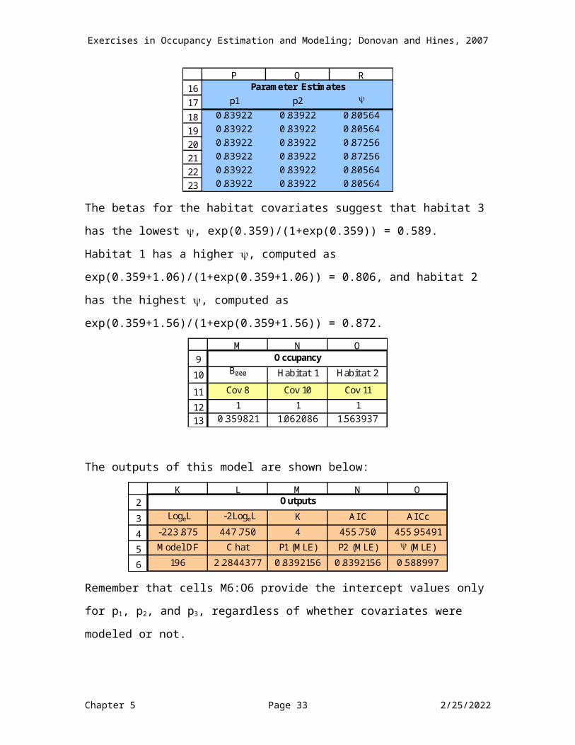
With a p1 and p2 intercept of 1.65, the probability of detecting a species, given it is present, is exp(1.65)/(1+exp(1.65)) = 0.839. You can see that p1 = p2 for all sites, as specified by the model. The estimates are shown below for the first 6 sites, and the estimate depends on what habitat they are located in.
1617181920212223
P Q R
p1 p2
0.83922 0.83922 0.805640.83922 0.83922 0.805640.83922 0.83922 0.872560.83922 0.83922 0.872560.83922 0.83922 0.805640.83922 0.83922 0.80564
Parameter Estimates
The betas for the habitat covariates suggest that habitat 3 has the lowest , exp(0.359)/(1+exp(0.359)) = 0.589. Habitat 1 has a higher , computed as exp(0.359+1.06)/(1+exp(0.359+1.06)) = 0.806, and
Chapter 5 Page 26 5/9/2023

Exercises in Occupancy Estimation and Modeling; Donovan and Hines, 2007
habitat 2 has the highest , computed as exp(0.359+1.56)/(1+exp(0.359+1.56)) = 0.872.
9
10
11
1213
M N O
B000 Habitat 1 Habitat 2Cov 8 Cov 10 Cov 11
1 1 10.359821 1.062086 1.563937
Occupancy
The outputs of this model are shown below:
2
3
4
5
6
K L M N O
LogeL -2LogeL K AI C AI Cc-223.875 447.750 4 455.750 455.95491Model DF C hat P1 (MLE) P2 (MLE) (MLE)
196 2.2844377 0.8392156 0.8392156 0.588997
Outputs
Remember that cells M6:O6 provide the intercept values only for p1, p2, and p3, regardless of whether covariates were modeled or not.
Now let’s look at model fit. On preliminary inspection, this model seems to fit the data fairly well. The Chi-Square for this model is 4.12; there are a few less 10 histories than were predicted by the model, and a few more 01 histories than predicted by the model:
3
4
5
6
7
8
9
10
T U V W
Observed Expected (O-E)2/ E11 107 107.0 0.00010 14 20.5 2.06101 27 20.5 2.06100 52 52.0 0.000
200 200 Chi-Square4.1220
MacKenzie- Bailey Goodness of Fit
0
0
0
0
0
1
1
1
1
1
1
0 1 1
Covariate (x)
Logi
t (ps
i)
0.0
0.1
0.2
0.3
0.4
0.5
0.6
0.7
0.8
0.9
1.0
0 0 0 1 1 1Covariate (x)
Psi
Add the results of this model to the Results Table by clicking on the checkbox associated with Model 1:
Chapter 5 Page 27 5/9/2023

Exercises in Occupancy Estimation and Modeling; Donovan and Hines, 2007
3
4
5
6
7
8
9
10
11
QADD
RESULTSModel 1Model 2
Model 3
Model 4
Model 5Model 6
Model 7
The checkboxes are simply a form option in Excel, and they are tied to a macro which copies the AICc score and pastes the value into the appropriate cell in the Results Table. Keep in mind that when you click one of these boxes (either on or off), you’ll paste in whatever the current AICc score is in cell O4 (so select the checkbox immediately after you run a model, or you might accidentally paste in the AICc score of a different model than you intended!).
MODEL 2: p1(int)p2(int)psi(habitat)OK, now let’s run a model where we estimate a unique intercept for p1 and p2, and neither will be a function of covariates. We’ll still constrain to be a function of habitat (as we will for all 7 models). Set up your spreadsheet as shown. Make sure that if a beta is not being estimated (either because it is not being considered in the model or because it is constrained to equal another beta), that you enter a 0 in row 12. Then enter either a 0 or an equation in the corresponding cells in row 13:
9
10
11
1213
F G H I J K L M N O
B0 Temp Rain B00 Temp Rain Recapture B000 Habitat 1 Habitat 2Cov 1 Cov 2 Cov 3 Cov 4 Cov 5 Cov 6 Cov 7 Cov 8 Cov 10 Cov 11
1 0 0 1 0 0 0 1 1 10.000000 0.000000 0.000000 0.000000 0
Survey 1 Survey 2 Occupancy
Chapter 5 Page 28 5/9/2023

Exercises in Occupancy Estimation and Modeling; Donovan and Hines, 2007
Now, run Solver again, maximizing cell but this time changing cells F13, I13, M13:O13:
Note that a unique intercept is estimated for p1 and p2. In this case, p1 = 0.79851 for all sites in survey 1, and p2 = 0.8843 for all sites in survey 2. Note also that the beta estimates from this model for occupancy are slightly different than the previous model, as would be expected because the data are being explained by 5 parameters in this model instead of 4.
9
10
11
1213
F G H I J K L M N O
B0 Temp Rain B00 Temp Rain Recapture B000 Habitat 1 Habitat 2Cov 1 Cov 2 Cov 3 Cov 4 Cov 5 Cov 6 Cov 7 Cov 8 Cov 10 Cov 11
1 0 0 1 0 0 0 1 1 11.376991 0.000000 0.000000 2.033770 0.000000 0.000000 0 0.353501 1.055088 1.550017
Survey 1 Survey 2 Occupancy
161718192021222324
P Q R
p1 p2
0.79851 0.88430 0.803540.79851 0.88430 0.803540.79851 0.88430 0.870290.79851 0.88430 0.870290.79851 0.88430 0.803540.79851 0.88430 0.803540.79851 0.88430 0.80354
Parameter Estimates
Add the results of this model to the Results Table by checking the check-box associated with Model 2. Your table should look like this:
Chapter 5 Page 29 5/9/2023

Exercises in Occupancy Estimation and Modeling; Donovan and Hines, 2007
3
4
5
6
7
8
9
10
11
12
X Y Z AA AB AC
Model AI Cc Rank Delta Exp(-0.5*Delta) Weight1. p(.)psi(habitat) 455.95 2 2.090 0.3517 0.00002. p1(int)p2(int)psi(habitat) 453.87 1 0.000 1.0000 0.00003. p1 = p2 (int), p1 = p2(temp),psi(habitat) #N/ A -453.865 ############ 0.20004. p1 = p2(int), p1(temp)p2(temp), psi(habitat) #N/ A -453.865 ############ 0.20005. p1(int)p2(int),p1 = p2 (temp), psi(habitat) #N/ A -453.865 ############ 0.20006. p1(int)p2(int),p1(temp),p2 (temp), psi(habitat) #N/ A -453.865 ############ 0.20007. p1(temp+rain)p2(temp+rain+trap response)psi(habitat) #N/ A -453.865 ############ 0.2000
Minimum AI C = 453.865 Sum = ############
Model Selection Results Table
So far, the model where the intercepts for p1 and p2 were uniquely estimated is the most parsimonious model.
MODEL 3: p1 = p2 (int), p1 = p2(temp), psi(habitat)In this model, we will force the intercepts and slopes for temperature to be equal for survey 1 and survey 2. The model is for temperature is similar to that shown below, but we’ll let Solver tell us what the intercept and slope really are.
-2
-1.5
-1
-0.5
0
0.5
1
1.5
2
2.5
3
-6 -4 -2 0 2 4 6
Standardized Temperature
Logi
t p1
and
logi
t p2
Logit p1 Logit p2
Thus, we only estimate 5 parameters for this model, two of which are associated with detection.
9
10
11
1213
F G H I J K L M N O
B0 Temp Rain B00 Temp Rain Recapture B000 Habitat 1 Habitat 2Cov 1 Cov 2 Cov 3 Cov 4 Cov 5 Cov 6 Cov 7 Cov 8 Cov 10 Cov 11
1 1 0 0 0 0 0 1 1 10 =F13 =G13 0 0
Survey 1 Survey 2 Occupancy
Go ahead and run this model, study the output. You’ll see that, as specified, the intercepts for survey 1 and 2 are the same, as is the slope of temperature. In this case, the effect of temperature is positive but very weak (0.062). In MARK or PRESENCE, you would also scrutinize the standard error associated with the estimates to determine how precise they are.
Chapter 5 Page 30 5/9/2023

Exercises in Occupancy Estimation and Modeling; Donovan and Hines, 2007
9
10
11
1213
F G H I J K L M N O
B0 Temp Rain B00 Temp Rain Recapture B000 Habitat 1 Habitat 2Cov 1 Cov 2 Cov 3 Cov 4 Cov 5 Cov 6 Cov 7 Cov 8 Cov 10 Cov 11
1 1 0 0 0 0 0 1 1 11.653848 0.062482 0.000000 1.653848 0.062482 0.000000 0 0.359206 1.064621 1.552461
Survey 1 Survey 2 Occupancy
Now add the results to your Results Table by clicking on the check-box next to Model 3:
3
4
5
6
7
8
9
10
11
12
X Y Z AA AB AC
Model AI Cc Rank Delta Exp(-0.5*Delta) Weight1. p(.)psi(habitat) 455.95 2 2.090 0.3517 0.00002. p1(int)p2(int)psi(habitat) 453.87 1 0.000 1.0000 0.00003. p1 = p2 (int), p1 = p2(temp),psi(habitat) 457.92 3 4.058 0.1315 0.00004. p1 = p2(int), p1(temp)p2(temp), psi(habitat) #N/ A -453.865 ############ 0.25005. p1(int)p2(int),p1 = p2 (temp), psi(habitat) #N/ A -453.865 ############ 0.25006. p1(int)p2(int),p1(temp),p2 (temp), psi(habitat) #N/ A -453.865 ############ 0.25007. p1(temp+rain)p2(temp+rain+trap response)psi(habitat) #N/ A -453.865 ############ 0.2500
Minimum AI C = 453.865 Sum = ############
Model Selection Results Table
MODEL 4: p1=p2(int)p1(temp)p2(temp)psi(habitat)In this model, we will force the intercepts for p1 to be equal to p2, but we will estimate a unique slope for each survey.
-10
-8
-6
-4
-2
0
2
4
6
8
10
-6 -4 -2 0 2 4 6
Standardized Temperature
Logi
t p1
and
logi
t p2
Logit p1 Logit p2
The set-up for this model is:9
10
11
1213
F G H I J K L M N O
B0 Temp Rain B00 Temp Rain Recapture B000 Habitat 1 Habitat 2Cov 1 Cov 2 Cov 3 Cov 4 Cov 5 Cov 6 Cov 7 Cov 8 Cov 10 Cov 11
1 1 0 0 1 0 0 1 1 10 =F13 0 0
Survey 1 Survey 2 Occupancy
Go ahead and run this model. Here are our results:
9
10
11
1213
F G H I J K L M N O
B0 Temp Rain B00 Temp Rain Recapture B000 Habitat 1 Habitat 2Cov 1 Cov 2 Cov 3 Cov 4 Cov 5 Cov 6 Cov 7 Cov 8 Cov 10 Cov 11
1 1 0 0 1 0 0 1 1 11.938463 1.249648 0.000000 1.938463 -0.803854 0.000000 0 0.353996 1.162156 1.538589
Survey 1 Survey 2 Occupancy
In this model, the intercept for p1 and p2 were identical (exp(1.94)/(1+exp(1.94))=0.87. However, the temperature beta for
Chapter 5 Page 31 5/9/2023

Exercises in Occupancy Estimation and Modeling; Donovan and Hines, 2007
survey 1 was positive (1.24), indicating that as the Z score for temperature increased, p1 increased, while the temperature beta for survey 2 was negative (-0.803), indicating that as the Z score for temperature increased, p2 decreased. Sites with Z scores of 0 for either survey had a 0.87 probability of detection, given the species was present. Add the results to the Results Table.
MODEL 5: p1(int)p2(int), p1=p2(temp)psi(habitat)OK, let’s keep going. In this model, we will estimate a unique intercept for p1 and p2, and we’ll estimate the temp effect, but the slope will be the same for both surveys.
-2
-1
0
1
2
3
4
5
-6 -4 -2 0 2 4 6
Standardized Temperature
Logi
t p1
and
logi
t p2
Logit p1 Logit p2
Set up your spreadsheet as follows, then maximize the log likelihood.9
10
11
1213
F G H I J K L M N O
B0 Temp Rain B00 Temp Rain Recapture B000 Habitat 1 Habitat 2Cov 1 Cov 2 Cov 3 Cov 4 Cov 5 Cov 6 Cov 7 Cov 8 Cov 10 Cov 11
1 1 0 1 0 0 0 1 1 10 =G13 0 0
Survey 1 Survey 2 Occupancy
Here are the results we got:
9
10
11
1213
F G H I J K L M N O
B0 Temp Rain B00 Temp Rain Recapture B000 Habitat 1 Habitat 2Cov 1 Cov 2 Cov 3 Cov 4 Cov 5 Cov 6 Cov 7 Cov 8 Cov 10 Cov 11
1 1 0 1 0 0 0 1 1 11.376980 0.072329 0.000000 2.038362 0.072329 0.000000 0 0.352797 1.057385 1.537999
Survey 1 Survey 2 Occupancy
This model suggests that survey 2 had a slightly higher overall probability of detection than survey 1, but in both surveys detection increased slightly as the Z score for temperature increased.
MODEL 6: p1(int)p2(int)p1(temp)p2(temp)psi(habitat)
Chapter 5 Page 32 5/9/2023
Exercises in Occupancy Estimation and Modeling; Donovan and Hines, 2007
OK, one more combination of intercepts and temperatures, then we’ll get to the recapture model. In this model, we will estimate a unique intercept and slope for each survey separately.
9
10
11
1213
E F G H I J K L M N O
B0 Temp Rain B00 Temp Rain Recapture B000 Habitat 1 Habitat 2Parameter Cov 1 Cov 2 Cov 3 Cov 4 Cov 5 Cov 6 Cov 7 Cov 8 Cov 10 Cov 11Estimate? 1 1 0 1 1 0 0 1 1 1Beta 0.000000 0.000000 0
OccupancySurvey 1 Survey 2
Run this model, and study the betas, and then add the results to the Results Table:
3
4
5
6
7
8
9
10
11
12
X Y Z AA AB AC
Model AI Cc Rank Delta Exp(-0.5*Delta) Weight1. p(.)psi(habitat) 455.95 5 29.716 0.0000 0.00002. p1(int)p2(int)psi(habitat) 453.87 3 27.626 0.0000 0.00003. p1 = p2 (int), p1 = p2(temp),psi(habitat) 457.92 6 31.684 0.0000 0.00004. p1 = p2(int), p1(temp)p2(temp), psi(habitat) 428.75 2 2.511 0.2849 0.00005. p1(int)p2(int),p1 = p2 (temp), psi(habitat) 455.81 4 29.576 0.0000 0.00006. p1(int)p2(int),p1(temp),p2 (temp), psi(habitat) 426.24 1 0.000 1.0000 0.00007. p1(temp+rain)p2(temp+rain+trap response)psi(habitat) #N/ A -426.239 ############ 1.0000
Minimum AI C = 426.239 Sum = ############
Model Selection Results Table
Let’s talk about this model overall. First, this model specifies that survey 1 is a function of temp, and survey 2 is a function of temp. We estimate a unique intercept and temperature slope for each survey. This model only makes sense if the survey periods do not overlap and instead have definitive groupings (e.g., if survey 1 took place in early breeding season, and survey 2 took place in the middle of the breeding season.). If the two surveys were not defined by some time period, in our mind this model would make little sense. If we surveyed the sites in a random order (with some sites having both surveys occur in the early breeding season, and other sites having both surveys occur in the middle of the breeding season, and still other sites with surveys occurring in both the early and middle portion of the breeding season), there is no reason to suspect that the intercepts and slopes would vary between the survey periods in a meaningful way. Keep this in mind when running survey-specific models. Survey-specific models are very appropriate, however, to account for observer differences (in which the field observer is a categorical covariate), or when you wish to model
Chapter 5 Page 33 5/9/2023

Exercises in Occupancy Estimation and Modeling; Donovan and Hines, 2007
some dependencies among the surveys (as we’ll see in the next model).
MODEL 7: p1(int+temp+rain)p2(int+temp+rain+recapture)psi(habitat)Last model! In this model, we’ll run a fully parameterized model: we’ll constrain p1 to be a function of its intercept, temperature, and rain, and we’ll constrain p2 to be a function of its intercept, temperature, rain, and recapture. The spreadsheet set up for this model is as shown:
9
10
11
1213
F G H I J K L M N O
B0 Temp Rain B00 Temp Rain Recapture B000 Habitat 1 Habitat 2Cov 1 Cov 2 Cov 3 Cov 4 Cov 5 Cov 6 Cov 7 Cov 8 Cov 10 Cov 11
1 1 1 1 1 1 1 1 1 1
Survey 1 Survey 2 Occupancy
Run this model, and then study your results.9
10
11
1213
F G H I J K L M N O
B0 Temp Rain B00 Temp Rain Recapture B000 Habitat 1 Habitat 2Cov 1 Cov 2 Cov 3 Cov 4 Cov 5 Cov 6 Cov 7 Cov 8 Cov 10 Cov 11
1 1 1 1 1 1 1 1 1 11.374383 0.922653 -0.133354 1.162958 -1.061997 -0.077562 1.412877086 0.460443 1.363276 1.870516
Survey 1 Survey 2 Occupancy
This model is similar to the previous model, except that rain is included as a covariate and the “recapture” effect is added to survey 2. Let’s focus only on the the p2 estimates to fully understand the “recapture” effect. In this model, the linear equation is:Logit p2 = 1.16*1 + -1.06*temp + -0.077*rain + 1.41*recapture. The effect of temperature is negative, and fairly strong; as Z score for temperature increases, p2 decreases. Rain also has a negative coefficient, but the effect size is pretty small (-0.077). The recapture covariate is very strong and positive (1.41), indicating that if the species was detected on survey 1 at a site, the probability of detecting it again on survey 2 was increased substantially. This can be seen readily by examining the p2 estimates of the first 4 sites:
Chapter 5 Page 34 5/9/2023

Exercises in Occupancy Estimation and Modeling; Donovan and Hines, 2007
161718192021
E I J K L P Q R
History P2 (I nt) Temp Rain Recapture p1 p2
01 1 0.677849685 0 0 0.46263 0.60899 0.8610101 1 1.610119806 0 0 0.67900 0.36656 0.8610111 1 -1.492037964 0 1 0.78739 0.98464 0.9114111 1 -0.409391906 0 1 0.81697 0.95305 0.91141
Survey 2 Covariates Parameter Estimates
Sites 1 and 2 had histories of 01, so there is no chance of a trap response. But sites 3 and 4 were detected in survey 1, and thus had a 1 in the “recapture” covariate. And their detection probabilities increased in survey 2 as a result of the beta being strong and positive, indicating the “trap happy” response. Add the results of this model to the Results Table, and we can now compare our 7 models.
3
4
5
6
7
8
9
10
11
12
X Y Z AA AB AC
Model AI Cc Rank Delta Exp(-0.5*Delta) Weight1. p(.)psi(habitat) 455.95 6 29.716 0.0000 0.00002. p1(int)p2(int)psi(habitat) 453.87 4 27.626 0.0000 0.00003. p1 = p2 (int), p1 = p2(temp),psi(habitat) 457.92 7 31.684 0.0000 0.00004. p1 = p2(int), p1(temp)p2(temp), psi(habitat) 428.75 2 2.511 0.2849 0.20705. p1(int)p2(int),p1 = p2 (temp), psi(habitat) 455.81 5 29.576 0.0000 0.00006. p1(int)p2(int),p1(temp),p2 (temp), psi(habitat) 426.24 1 0.000 1.0000 0.72657. p1(temp+rain)p2(temp+rain+trap response)psi(habitat) 431.02 3 4.782 0.0916 0.0665
Minimum AI C = 426.239 Sum = 1.3765
Model Selection Results Table
MODEL SELECTION ANALYSISNow let’s compare the results from the different models. Why compare these models? Well, we want to determine which model best “fits” our observed data so that we can infer something about detection probability and probability of site occupancy – the purpose of occupancy model. You probably know by now that in many cases you can fit models better by estimating more parameters. The model selection paradigm (presented by Ken Burnham and David Anderson in their book, Model Selection and Multimodel Inference) uses AICc as a measure of parsimony – and this consists of a measure of fit of the data (-2LogeL) and the number of parameters (K): AIC = -2LogeL + 2K. (AICc is a second order correction of AIC). In the words of Cooch and White, “AICc is a good, well-justified criterion for selecting the most parsimonious model, i.e., the model which best explains the variation in the data while using the fewest parameters.” For two models, the
Chapter 5 Page 35 5/9/2023

Exercises in Occupancy Estimation and Modeling; Donovan and Hines, 2007
one with the lower AICc value is considered a more parsimonious model. As you add parameters to a certain model, the -2LogeL may get smaller (the model fit may be better), but the number of parameters is increased. As a result, as you add parameters to a model, its bias is reduced but the variance in each parameter is increased, such that precision is lost. So there is a trade-off in how well the model fits the data and the number of parameters that need to be estimated. Also, from a practical perspective, in many cases estimating the value of an additional parameter is a costly enterprise, so we want a model that explains the data well while at the same time keeps the number of parameters that need to be estimated at a minimum. The model selection paradigm provides a method for comparing model AICc scores as a means for weighing the evidence of competing models. Let’s compare the models now:
3
4
5
6
7
8
9
10
11
12
X Y Z AA AB AC
Model AI Cc Rank Delta Exp(-0.5*Delta) Weight1. p(.)psi(habitat) 455.95 6 29.716 0.0000 0.00002. p1(int)p2(int)psi(habitat) 453.87 4 27.626 0.0000 0.00003. p1 = p2 (int), p1 = p2(temp),psi(habitat) 457.92 7 31.684 0.0000 0.00004. p1 = p2(int), p1(temp)p2(temp), psi(habitat) 428.75 2 2.511 0.2849 0.20705. p1(int)p2(int),p1 = p2 (temp), psi(habitat) 455.81 5 29.576 0.0000 0.00006. p1(int)p2(int),p1(temp),p2 (temp), psi(habitat) 426.24 1 0.000 1.0000 0.72657. p1(temp+rain)p2(temp+rain+trap response)psi(habitat) 431.02 3 4.782 0.0916 0.0665
Minimum AI C = 426.239 Sum = 1.3765
Model Selection Results Table
First, we find the model with the lowest AICc score – this is the most parsimonious model. In this case, it happens to be model 6, p1(int)p2(int),p1(temp),p2 (temp), psi(habitat). The lowest AICc score of the seven is calculated in cell Y12 with a MIN function. Cells Z5:Z11 rank the models from best to worst with a RANK function. You can see that model 6 was ranked first, followed by the model where the intercepts for p1 and p2 were constant but their slopes were uniquely estimated.
Chapter 5 Page 36 5/9/2023

Exercises in Occupancy Estimation and Modeling; Donovan and Hines, 2007
3
4
5
6
7
8
9
10
11
12
X Y Z AA AB AC
Model AI Cc Rank Delta Exp(-0.5*Delta) Weight1. p(.)psi(habitat) 455.95 6 29.716 0.0000 0.00002. p1(int)p2(int)psi(habitat) 453.87 4 27.626 0.0000 0.00003. p1 = p2 (int), p1 = p2(temp),psi(habitat) 457.92 7 31.684 0.0000 0.00004. p1 = p2(int), p1(temp)p2(temp), psi(habitat) 428.75 2 2.511 0.2849 0.20705. p1(int)p2(int),p1 = p2 (temp), psi(habitat) 455.81 5 29.576 0.0000 0.00006. p1(int)p2(int),p1(temp),p2 (temp), psi(habitat) 426.24 1 0.000 1.0000 0.72657. p1(temp+rain)p2(temp+rain+trap response)psi(habitat) 431.02 3 4.782 0.0916 0.0665
Minimum AI C = 426.239 Sum = 1.3765
Model Selection Results Table
The delta column (cells AA5:AA11) computes the difference in AICc scores between the best model (rank = 1) and the other models. So the best ranked model will always have Delta = 0. If the delta values are within 2 AICc units of the best ranking model, there is strong evidence of support for both that model and for the best ranked model. If the delta values are between 2 and 7, then there is considerable support for that model as well as the top ranked model. See Burnham and Anderson for a much more thorough and better-explained discussion of this topic. So, for this dataset, three of the seven models appear to be supported by the data, models 4, 6, and 7. While it’s nice to have a single model “blow the other models away” to keep interpretation nice and clean, it’s often the case in ecological studies where there is support for multiple models, as is the case here. However, you can see that models 4, 6, and 7 blow the other models out of the water, such that we don’t need to consider them further. Their delta scores (all > 15) indicate that they are much less supported than the top ranked model.
The weight of evidence (cells AC5:AC11) for each model is computed with two steps. First, we take the exponent of -1/2 times the delta value for each model (cells AB5:AB11). Why? Because awhile ago we multiplied by log likelihood by -2 (Akaike did this for historical reasons), and to get back to the basic likelihood we need to take the exponent (which negates the log) and multiply by -1/2 (which negates the multiplication by -2). Then these scores are added (cell AB12). Then
Chapter 5 Page 37 5/9/2023

Exercises in Occupancy Estimation and Modeling; Donovan and Hines, 2007
the Akaike weights are computed in cells AC5:AC11 as the model's EXP (-1/2 * delta) score divided by the sum (cell AB12). These weights are interpreted as probability of being the best K-L model in the model set. From these weights, you can see if one model has most of the support, or if several models explain the data equally well. So, for our example, model 6, p1(int)p2(int),p1(temp),p2 (temp), psi(habitat) has an AIC weight of 0.7265, indicating that this model has a 72.65% chance of being the best K-L model in the model set. The next best-supported model is the model 4: p1 = p2(int), p1(temp)p2(temp), psi(habitat), with an AIC weight of 0.2070, indicating that it has a 20.70% chance of being the best K-L model in the model set. And model 7 had a 6.65% of being the best model in model set. In this example, you probably wouldn’t bet your lunch on any one model as being the best model, but you could bet your lunch that either model 4, 6, or 7 is the best model in the model set.
Now, we’ve run 7 models, and have drawn some conclusions using model selection procedures. What’s next? Well, in case you don’t remember, at this point you should run a MacKenzie and Bailey GOF bootstrap to determine if at least one model in the model sets fits the data. In other words, we’ve found support for three models, but what if neither of these really explains the histories we observed in the study? This exercise is already long enough, but we challenge you to program in a bootstrap model and then run the GOF test.
MODEL AVERAGING AND MULTI-MODEL INFERENCESo, as a quick summary, we used model selection procedures to compare the AICc scores among the seven models we ran, and we found substantial support for two of them, and virtually no support for the others. Each model provided us with some parameter estimates for drawing inferences about detection probability and probability of
Chapter 5 Page 38 5/9/2023

Exercises in Occupancy Estimation and Modeling; Donovan and Hines, 2007
occupancy. We know that none of the models gives the “correct” estimates, but which ones should we report? Is there a way to use the information from the model selection process and not disregard the information from any model? The answer is yes, and the process is called model averaging. Basically, there are 200 sites, and each of the 7 models estimated a p1, p2, and psi for each site. How could you get a model averaged estimate for each site? Simple! You run model 1, get the estimates for p1, p2, and psi for each site, and then multiple those estimates by the model’s AICc weight. Then you run model 2, get the estimates of p1, p2, and psi for each site, and then multiple those estimates by model 2’s AICc weight. You do the same thing for models 3 - 7. Though you might not have realized it, we’ve been tracking the model-specific estimates of p1, p2, and for each site on the worksheet labeled “Averages”. Let’s take a look at that worksheet now.
Each time you ran a model and added the results to the Results Table, the spreadsheet copied the site-specific estimates of p1, p2, and from that model. The estimates from the first three models are shown for the first five study sites:
3456789
A B C D E F G H I J K L M
Site p1 p2 Weight p1 p2 Weight p1 p2 Weight1 0.839216 0.839216 0.805637 2.56E-07 0.798507 0.884297 0.803543 7.28E-07 0.825005 0.845038 0.805938 9.58E-082 0.839216 0.839216 0.805637 2.56E-07 0.798507 0.884297 0.803543 7.28E-07 0.833621 0.852513 0.805938 9.58E-083 0.839216 0.839216 0.872557 2.56E-07 0.798507 0.884297 0.870289 7.28E-07 0.840032 0.826443 0.871206 9.58E-084 0.839216 0.839216 0.872557 2.56E-07 0.798507 0.884297 0.870289 7.28E-07 0.840517 0.835932 0.871206 9.58E-085 0.839216 0.839216 0.805637 2.56E-07 0.798507 0.884297 0.803543 7.28E-07 0.832792 0.838424 0.805938 9.58E-08
Model 1 Model 2 Model 3
Remember that model 1 forced p1 = p2 with no covariates while model 2 estimated the intercepts for p1 and p2 only. Model 3 estimated p as function of temperature, so the 5 sites shown have different estimates for p1 and p2 depending on the temperature in which the survey was conducted.
Chapter 5 Page 39 5/9/2023

Exercises in Occupancy Estimation and Modeling; Donovan and Hines, 2007
Next to each of the parameter estimates, the AIC weight associated with each model is provided. Click on cell E5 and you’ll see the formula ='Survey Covariates'!$AC$5, which simply grabs the AIC weight from the Results Table.
Now scroll over to columns AD:AF and you’ll see the model averaged estimates for each site:
3456789
AD AE AF
p1 p2
0.476992339 0.824714307 0.8178850.715055623 0.648020276 0.8178850.843326125 0.978957858 0.8732480.85237001 0.941083965 0.8732480.692463335 0.922236566 0.817885
MODEL AVERAGED ESTIMATES
Click on cell AD5 and you’ll see the formula for computing the model averaged estimate of p1 for site 1: =B5*E5+F5*I5+J5*M5+N5*Q5+R5*U5+V5*Y5+Z5*AC5. Click on the formula in the formula bar and you’ll see the cells used in the equation light up. This equation simply multiplies the estimate from each model by that model’s AIC weight, and then adds the results up across all seven models.
SIMULATING SURVEY-SPECIFIC COVARIATE DATAOK! We’re finally closing in the end of the site-level covariate exercise. We’ve covered a LOT of ground, but we still need to learn how to simulate data for analysis. Click back on the sheet labeled “Survey Covariates,” scroll to the right of the sheet, and you’ll find a section labeled Simulate Data:
Chapter 5 Page 40 5/9/2023

Exercises in Occupancy Estimation and Modeling; Donovan and Hines, 2007
The parameters for this model are listed in cells AG11:AP12. All you need to do is enter some beta values in cells AG13:AP13, and then press F9 to simulate new data. The beta values shown below are the actual values used to simulate the data we’ve been analyzing. Thus, we simulated data where there is a date and rain effect on p1 and p2 (and these are survey specific), plus there is a strong “trap-happy” response where the detection rate at a site during survey 2 significantly increases if the species was detected in survey 1. Of course, there is habitat effect on . Note that this exact model was not included in the model set.
10
11
1213
AF AG AH AI AJ AK AL AM AN AO AP
B0 Temp Rain B00 Temp Rain Recapture B00 Habitat 1 Habitat 2Parameter P (I nt) Cov 2 Cov 3 Psi (I nt) Cov 5 Cov 6 Cov 7 Psi (I nt) Cov 10 Cov 11
Beta 1.00 1.00 0.00 0.50 -1.00 0.00 2.00 0.50 0.30 1.50
OccupancySurvey 2Survey 1
Now, let’s assign some covariate values to each site:171819202122
AF AG AH AI AJ AK AL AM AN AO APSite P (I nt) Temp Rain B00 Temp Rain Recapture B00 Habitat 1 Habitat 2
1 1 1.88799563 0 1 -0.519902 1 1 1 0 12 1 1.321585121 1 1 0.554163 0 1 1 1 03 1 0.430858798 0 1 1.135436 1 1 1 1 04 1 0.734176276 1 1 1.366277 0 1 1 0 15 1 0.2345754 0 1 -0.662155 0 0 1 1 0
Chapter 5 Page 41 5/9/2023

Exercises in Occupancy Estimation and Modeling; Donovan and Hines, 2007
The sites are listed in column AF, and in AG we assign a 1 for the intercept of p1. Cov 2 (temp) is continuous variables, so we need to enter a Z score for each site. The formulae in cells AH18 generates Z scores for site 1 with the equation =NORMSINV(RAND()), which generates a random Z score from a distribution whose mean is 0 and whose standard deviation is 1. This formula is copied down for the remaining sites. Cov 3 (rain) is categorical, where 1 = rain and 0 = no rain. The formula in cell AI18 generates a 1 or 0 for site 1 with the formula =IF(RAND()<0.5,1,0). This formula draws a random number, and if the random number is less that 0.5, a 1 results, otherwise a 0 results. In this way, we are creating data for each site in a random fashion.
For p2, we enter a 1 in column AJ for the intercept for all sites. In column AK we again use the =NORMSINV(RAND()) function to generate a random Z score to assign a temperature associated with survey 2. In column AL we use the =IF(RAND()<0.5,1,0) to assign a rain category associated with survey 2. The covariate “recapture” is not assigned with random numbers, but rather is assigned based on the outcome of survey 1. In the spreadsheet, click on cell AM18 and you’ll see the formula =AW18. Cell AW18 assigns an encounter history for survey 1….if the species was detected on survey 1, the covariate “recapture” is scored 1; otherwise it is scored 0. We’ll come back to this in a minute.
Generating the psi covariates is a bit trickier (but only a little), due to the fact that habitat is coded by 2 covariates. In column AN, we enter a 1 for the intercept for habitat for all sites. In column AO and AP, we enter a 1 or 0 to obtain habitat covariates for each site. In cell AO18, the formula is =IF(RAND()<0.33,1,0). This function draws a random number, and if the random number is less than 0.33, a 1 is returned,
Chapter 5 Page 42 5/9/2023

Exercises in Occupancy Estimation and Modeling; Donovan and Hines, 2007
indicating that that site is located in habitat 1. In cell AP18, we entered the equation =IF(AO18=1,0,IF(RAND()<0.5,1,0)) to generate values for habitat 2. This function is 2 IF functions. The first function, =IF(AO18=1,0 looks at the result in cell AO18 (habitat 1), and if the answer is 1 then the spreadsheet returns a 0 under the habitat 2 column (a site cannot be both habitat 1 and habitat 2 at the same time). If habitat 1 is not 1, the equation moves to the second function: IF(RAND()<0.5,1,0)) . If a random number is less than 0.5, a 1 is returned, indicating that the site is located in habitat 2. If the random number greater than 0.5, then a 0 is returned. In this way, we roughly assign habitats to the 200 sites in roughly equal numbers.
An important thing to notice here is that the assignments for the various covariates values for site 1 are completely independent of each other. That is, the Z score for Cov 1 does not depend on any of the other covariate values for site 1 (we haven’t simulated data where one covariate value depends on the value of another covariate. That is, we haven’t simulated data that “interact” in any way, nor are they correlated).
Now that each site has covariate values, and beta values specified in cells AG13:AP13, we can compute each site’s and p parameters as we’ve done previously, and we can simulate data in the same way we simulated data for the bootstrap. For site 1, p1 is computed in cell AQ18 with the equation =EXP(SUMPRODUCT($AG$13:$AI$13,AG18:AI18))/(1+EXP(SUMPRODUCT($AG$13:$AI$13,AG18:AI18)))), which is the back-transformed logit equation. For site 1, p2 is computed in cell AR18 with the equation =EXP(SUMPRODUCT($AJ$13:$AM$13,AJ18:AM18))/(1+EXP(SUMPRODUCT($AJ$13:$AM$13,AJ18:AM18))), which is the back-transformed logit equation for p2. Site 1’s is computed in cell AS18 with the equation
Chapter 5 Page 43 5/9/2023
Exercises in Occupancy Estimation and Modeling; Donovan and Hines, 2007
=EXP(SUMPRODUCT($AN$13:$AP$13,AN18:AP18))/(1+EXP(SUMPRODUCT($AN$13:$AP$13,AN18:AP18))). Remember, the results from these equations are completely dependent on the site’s covariate values and the beta values you enter. Columns AT:AV are simply random numbers, and columns AW:AY simply use the random numbers to create histories based on the site’s p1, p2, and values (as determined by the betas entered and covariate values). Take some time to look at the spreadsheet equations before moving on.
CREATING INPUT FILES FOR MARK AND PRESENCEThe final step is to compare your spreadsheet result with results generated in MARK and PRESENCE. To develop a MARK input file, select cells Y18:Y217, and copy them into Notepad.
Save this file with an INP extension (e.g., “Occupancy_Survey_Covariates.inp”), and we’ll import this file into MARK later on.
To create an input file for PRESENCE, we’ll simply copy and paste the raw data provided on the spreadsheet.
Chapter 5 Page 44 5/9/2023

Exercises in Occupancy Estimation and Modeling; Donovan and Hines, 2007
SINGLE-SPECIES, SINGLE-SEASON OCCUPANCY WITH SURVEY COVARIATES IN PROGRAM PRESENCE
INPUT DATAIn this exercise, we will analyze the data in the spreadsheet Survey Covariates in program PRESENCE. Remember that this worksheet has only two sampling sessions, with survey-specific covariates for p1 and p2, and site-level covariates associated with occupancy (habitat). Remember, site-level covariates never change over the study – a site’s habitat cannot change from habitat 1 to habitat 2 in the study. (If it could, habitat would be considered a survey-level covariate).
Open PRESENCE and go to File | New. In the Enter Specifications Form, we’ll create the PRESENCE input file. Enter a title for the analysis (e.g., Occupancy with Site + Survey Covariates). Enter 200 for the number of sites, and 2 for the number of occasions. Now tell PRESENCE that there are 3 sampling or survey-specific covariates (temp, rain, and the p2 recapture) and 2 site-level covariates (habitat1, habitat2).
When you are finished, click on the button labeled “Input Data Form”. PRESENCE then presents you with the Data Input Form, where you can paste in your data.
Chapter 5 Page 45 5/9/2023

Exercises in Occupancy Estimation and Modeling; Donovan and Hines, 2007
Notice that Data Input Form consists of several tabs. The first tab (called Presence/Absence data) is where you enter the encounter histories. Return to your spreadsheet, and copy cells C18:D217. Then select the first empty data cell on the PRESENCE Data Input Form, and go to Edit | Paste | Paste Values.
Now click on the tab labeled “Site Covars”. Our site-level covariates include habitat only. On the spreadsheet, select cells N17:O217, and copy them. Then select the Data Input Form again, and select the first box of data, and go to Edit | Paste | Paste w/covnames.
Your Data Input Form should look like this:
Chapter 5 Page 46 5/9/2023

Exercises in Occupancy Estimation and Modeling; Donovan and Hines, 2007
OK, now we have to paste in the survey-specific (or sampling) covariates. As you can see, each covariate has a tab. Let’s call SampCov1 “temperature.” Return to your spreadsheet, and copy cells Z17:AA217. These are the same data we’ve been working with only ordered in a way that we can directly copy them into PRESENCE. Make sure that you include the covariate name in the data, and select Paste | Paste Values with Covariate Name.
Now, it’s not very helpful to have a tab labeled SampCov1, so click on the tab itself and then go to Edit | Rename Covariate, and type in the word “Temperature” in the dialogue box, and then press OK.
Chapter 5 Page 47 5/9/2023
Exercises in Occupancy Estimation and Modeling; Donovan and Hines, 2007
Your tab should now read Temperature:
PRESENCE will refer to the temperature covariates as TEMPERATURE, rather than p1_temp and p2_temp. It knows that the data in the first column pertain to the first survey period, and that the data in the second column pertain to the second survey period. Keep this in mind when we run models using the Design Matrix later on.
Repeat this process for Rain (SampCov2; cells AB17:AC217) and Recapture (SampCov3; cells AD17:AE217). Your input form should look as follows, with each of the five tabs holding the appropriate data.
Chapter 5 Page 48 5/9/2023
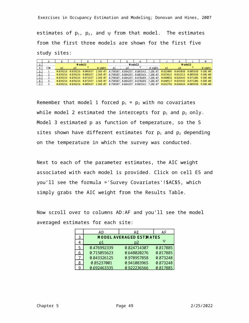
Exercises in Occupancy Estimation and Modeling; Donovan and Hines, 2007
When you are finished, you’ll need to save this file as the PRESENCE input file. Go to File | Save As, and save the file as “Occupancy with Site + Survey Covs.pao” (don’t include the quotation marks) and put it somewhere where you can retrieve it.
Click Save. Now, you can close the Input Data Form. Return to the Enter Specifications form and tell PRESENCE where the data is located. Click on the button labeled “Click to select file”, and then navigate to the location where you stored your .pao file.
Chapter 5 Page 49 5/9/2023

Exercises in Occupancy Estimation and Modeling; Donovan and Hines, 2007
Click OK, and PRESENCE then shows the Results Browser and your data is now ready for analysis.
MODEL 1: p(.)psi(habitat)The first model we’ll run is the p dot model, where all sites will have the same estimate for p, but where is a function of habitat ( will be a function of habitat for all 7 models that we’ll run). On the PRESENCE main menu, select Run | Analysis, Single-Season from the menu. Enter the name of the model you’ll be running (e.g., p(.)psi(habitat)), and then select the Custom radio button. You’ll be brought to the Design Matrix:
Chapter 5 Page 50 5/9/2023

Exercises in Occupancy Estimation and Modeling; Donovan and Hines, 2007
Now, there are many ways to specify a model in PRESENCE, and almost certainly you’ll find your own style. But for instruction purposes, we are going to build our models step-by-step. Note that there are two tabs. As shown above, the Occupancy tab is selected, so here is where we will specify a model that constrains to be a function of habitat type. What is currently shown is the intercept for psi, and PRESENCE calls this a1 (we called it B0 in the spreadsheet…don’t let that confuse you…just go with the flow). So, for us to specify a model where is a function of habitat, start by writing out the logit model for :
Logit = a1 + a2 * habitat1 + a3*habitat 2.So to estimate for each site, we need to estimate 3 parameters: a1, a2, and a3. Our Design Matrix has only one column in it at the moment, so we need to add two more. Click on the cell under a1, and right-click on your mouse. You should see the following options appear:
Select the “Add Cols” option, and then type in 2 to add two new columns. Your DM should look like this:
Chapter 5 Page 51 5/9/2023

Exercises in Occupancy Estimation and Modeling; Donovan and Hines, 2007
OK, remember, we are aiming to build the following model in the DM:Logit = (a1 * 1) + (a2 * habitat1) + (a3*habitat 2).
So we need to specify that a2 will be multiplied by the site’s data for habitat1, and we need to specify that a3 will be multiplied by the site’s data for habitat2. To initialize this model, click on the blank cell under a2, then go to the Init toolbar:
You’ll see that PRESENCE lists the site-level covariates by name (Habitat1 and Habitat2), and it lists the survey-level covariates by generalized name (e.g., Temperature instead of p1_temp and p2_temp). Select Habitat_1. Then click on the box under a3, and initialize it with Habitat_2. Your DM should look like this,
Chapter 5 Page 52 5/9/2023

Exercises in Occupancy Estimation and Modeling; Donovan and Hines, 2007
which specifies the model: Logit = (a1 * 1) + (a2 * habitat1) + (a3*habitat 2)
OK, that’s it for the occupancy side of the model. Now click on the tab labeled “Detection.”
You’ll notice that the Detection tab has a single beta associated with it (called b1), and that there is a “1” listed for both p1 and p2. This stacking indicates that b1 applies to both p1 and p2, and hence this is the “dot” model where the intercept for p1 = the intercept for p2. Our model is:
Logit p1 = 1 * b1Logit p2 = 1 * b1.
Now you are ready to run this model. Return to the Numerical Estimation Run page, and select OK.
Chapter 5 Page 53 5/9/2023

Exercises in Occupancy Estimation and Modeling; Donovan and Hines, 2007
When PRESENCE finished the analysis, it will bring up the following dialogue box:
Click Yes, and the results of this model will be added to the Results Browser.
To view the model’s results, just right-click on model name, and select an option that allows you to view the results:
Chapter 5 Page 54 5/9/2023

Exercises in Occupancy Estimation and Modeling; Donovan and Hines, 2007
Now, let’s work through the output, comparing the results to the spreadsheet. PRESENCE lists the number of groups (1, because this is not a mixture model), the number of sites (200), the number of sampling occasions (2), and the number of missing observations (0). In this model, we estimated 4 parameters: the intercept for p and three parameters associated with . The -2LogeL for this model is 447.75, and the AICc score is 455.75. All of these outputs match the spreadsheet.
2
3
4
5
6
K L M N O
LogeL -2LogeL K AI C AI Cc-223.875 447.750 4 455.750 455.9549109Model DF C hat P1 (MLE) P2 (MLE) (MLE)
196 2.284437667 0.83921564 0.839215641 0.588997027
Outputs
The naïve occupancy estimate from PRESENCE is 0.740. This is the proportion of sites in which at least one of the two surveys resulted in a detection. We could get that by adding the frequency of 11, 10, and 01 sites together, and then dividing by the total number of sites: (107 + 14 + 27)/200 = 0.740. PRESENCE then lists the beta estimates with the standard errors. You can see that the betas also match the spreadsheet; the occupancy betas are shown below:
Chapter 5 Page 55 5/9/2023

Exercises in Occupancy Estimation and Modeling; Donovan and Hines, 2007
9
10
11
1213
M N O
B000 Habitat 1 Habitat 2Cov 8 Cov 10 Cov 11
1 1 10.359821 1.062086 1.563937
Occupancy
Remember, it is critical that you evaluate not only the parameter estimate, but also the standard errors. Importantly, if the model does not fit the observed data, the standard errors may be too small, and can lead you down the dark side in terms of interpreting your data.
MODEL 2: p1(int)p2(int)psi(habitat)OK, now let’s try the same model, but where a separate intercept is estimated for p1 and p2. Return to the PRESENCE’s main page (with the picture on it), and go to Run | Analysis: Single Season. Enter a name for this model (e.g., Model 2: 2. p1(int)p2(int)psi(habitat), and then select the Custom radio button:
You’ll be presented with a fresh Design Matrix. Again, we’ll force to be a function of habitat. Start with the logit equation:
Chapter 5 Page 56 5/9/2023

Exercises in Occupancy Estimation and Modeling; Donovan and Hines, 2007
Logit y = a1*1 + a2*Habitat_1 + a3*Habitat_2. Use the right-click mouse button to add two columns, and initialize the DM so that you can “read” the logit equation across the row in the DM:
OK! Now, click on the detection tab.
The tab labeled Detection is where you specify a model constraining the two detection parameters, p1 and p2. If your data consisted of three survey occasions, three parameters would appear. So, the rows in the DM indicate the parameter name; in this case, there are two parameters, p1 and p2. In contrast, the columns of DM specify the linear model associated with a given parameter. That is, the columns represent the betas. In this model, we need to estimate a separate intercept for p1 and p2. The fastest way to get there is to go to Init | Full Identity:
Chapter 5 Page 57 5/9/2023

Exercises in Occupancy Estimation and Modeling; Donovan and Hines, 2007
And PRESENCE returns the following:
Thus, we have now specified the following single-season occupancy model:Logit = a1 * 1Logit p1 = b1 * 1Logit p2 = b2 * 1
That’s all! Return to the Setup page and run this model.
These results also match the spreadsheet results. Take some time to compare them before moving on. Now let’s move onto the more interesting models.
Chapter 5 Page 58 5/9/2023

Exercises in Occupancy Estimation and Modeling; Donovan and Hines, 2007
MODEL 3: p1 = p2 (int), p1 = p2(temp), psi(habitat)OK, the next four models consist of varying combinations of p1 intercept, p2 intercept, p1 temp, and p2 temp constraints. We’ll go through these in the same order as we did in the spreadsheet. In this model, we’ll force the intercepts of p1 and p2 to be equal, and we’ll let p1 and p2 be a function of temperature, but we’ll force the slopes to be equal.
Go ahead and start a new analysis, and name the model appropriately. Then set up the DM as we’ve done previously to constrain occupancy to be a function of habitat. Then, flip to the detection tab. OK, let’s start with the logit equations for p1 and p2:
Logit p1 = b1 *1 + b2 * temp1Logit p2 = b1 * 1 + b2 * temp2.
The intercepts for both p1 and p2 will be estimated by b1, and the slopes for temp1 and temp2 will be estimated by b2. So add one column to the DM. Then we initialize the data in this column by going to Init | Temperature. By default, PRESENCE stacks them in the DM.
This is perfect because the stacking indicates that b1 pertains to the intercepts for both p1 AND p2, and indicates that b2 pertains to the
Chapter 5 Page 59 5/9/2023

Exercises in Occupancy Estimation and Modeling; Donovan and Hines, 2007
slopes of temperature for both p1 AND p2. Go ahead and run this model.
Let’s take a look at the output:
And the spreadsheet results should match:2
3
4
5
6
7
8
9
10
11
1213
F G H I J K L M N O
11 10 01 00 Total LogeL -2LogeL K AI C AI Cc107 14 27 52 200 -223.807 447.614 5 457.614 457.9229428
Model DF C hat P1 (MLE) P2 (MLE) (MLE)195 2.295454689 0.8394105 0.839410504 0.588848309
B0 Temp Rain B00 Temp Rain Recapture B000 Habitat 1 Habitat 2Cov 1 Cov 2 Cov 3 Cov 4 Cov 5 Cov 6 Cov 7 Cov 8 Cov 10 Cov 11
1 1 0 0 0 0 0 1 1 11.653848 0.062482 0.000000 1.653848 0.062482 0.000000 0 0.359206 1.064621 1.552461
Summarized Inputs Outputs
OccupancySurvey 1 Survey 2
Take a look at the output from PRESENCE and make sure you understand what each piece is telling you.
MODEL 4: p1=p2(int)p1(temp)p2(temp)psi(habitat)
Chapter 5 Page 60 5/9/2023

Exercises in Occupancy Estimation and Modeling; Donovan and Hines, 2007
This next model is only slightly more difficult. Here, we force the intercepts for p1 and p2 to be equal, but will estimate the effect of temperature differently for p1 and p2. That is, the slopes can vary. Again, occupancy will be a function of habitat. Start a new analysis, and give the new analysis an appropriate title. Then set up the occupancy model as we’ve done previously, and then click on the detection tab. Let’s think about how many detection parameters will be estimated: one for the intercept, and two more for the survey-specific temperature effect. So add two more columns to the DM. Now, this time, when you initialize your model with Temperature, PRESENCE presents the default, stacked values.
This won’t work. Our logit equations are:Logit p1 = b1 *1 + b2 (temp1)Logit p2 = b1 * 1 + b3 (temp2)PRESENCE knows that “Temperature” in the p1 row refers to temp1, and that “Temperature” in the p2 row refers to temp2. But we need to scoot the word “Temperature” for p2 over into the b3 column. You can do this a few different ways; one way is to enter 0’s into the DM and type in the word “Temperature” directly:
Chapter 5 Page 61 5/9/2023

Exercises in Occupancy Estimation and Modeling; Donovan and Hines, 2007
Now you can run this model.
We know that this model is supported by the data from our spreadsheet exercise, so let’s study the output (the spreadsheet results are also shown).
Chapter 5 Page 62 5/9/2023

Exercises in Occupancy Estimation and Modeling; Donovan and Hines, 2007
2
3
4
5
6
7
8
9
10
11
1213
F G H I J K L M N O
11 10 01 00 Total LogeL -2LogeL K AI C AI Cc107 14 27 52 200 -208.158 416.315 6 428.315 428.7502813
Model DF C hat P1 (MLE) P2 (MLE) (MLE)194 2.145953856 0.87418323 0.874183229 0.587586213
B0 Temp Rain B00 Temp Rain Recapture B000 Habitat 1 Habitat 2Cov 1 Cov 2 Cov 3 Cov 4 Cov 5 Cov 6 Cov 7 Cov 8 Cov 10 Cov 11
1 1 0 0 1 0 0 1 1 11.938463 1.249648 0.000000 1.938463 -0.803854 0.000000 0 0.353996 1.162156 1.538589
Summarized Inputs Outputs
OccupancySurvey 1 Survey 2
First of all, let’s quickly review the occupancy estimates. Remember that we have three habitats, and that the reference habitat is habitat 3. The probability of occupancy for habitat 3 is exp(.354)/(1+exp(.354), or 0.5857. The probability of occupancy for habitat 1 is exp(0.354+1.16)/(1+( exp(0.354+1.16)), or 0.819. The probability of occupancy for habitat 2 is exp(0.354+1.54)/(1+( exp(0.354+1.54)), or 0.869. The beta associated with the detection intercept is 1.94. The slope for survey 1 is positive (1.25), while the slope for survey 2 is negative (-0.803). If we were to diagram the back-transformed logit equations, the results would look like this:
0
0.1
0.2
0.3
0.4
0.5
0.6
0.7
0.8
0.9
1
-5 -4 -3 -2 -1 0 1 2 3 4 5
Standardize Temperature
Dete
ctio
n Pr
obab
ility
p1
p2
Note that the intercept is equal for both p1 and p2, as specified by the model.
Chapter 5 Page 63 5/9/2023

Exercises in Occupancy Estimation and Modeling; Donovan and Hines, 2007
MODEL 5: p1(int)p2(int), p1=p2(temp)psi(habitat)In the next model, we’ll estimate a unique intercept for p1 and p2, but will force the slope for temperature to be the same for both groups. See if you can set this model up in the DM. Don’t forget to constrain to be a function of habitat.
The detection side of the DM should look like this:
Go ahead and add the results:
MODEL 6: p1(int)p2(int)p1(temp)p2(temp)psi(habitat)We’re almost done..two more to go. In this model, we’ll estimate the intercepts and temperature slopes for p1 and p2 uniquely (with occupancy as a function of habitat). Go ahead and run this model. The detection DM should look like this:
Chapter 5 Page 64 5/9/2023

Exercises in Occupancy Estimation and Modeling; Donovan and Hines, 2007
So our logit equations in PRESENCE are:Logit p1 = b1 * 1 + b3 (temp1)Logit p2 = b2 * 1 + b4 (temp2).Make sense? We hope so! Go ahead and run this model.
This is our top-ranked model…let’s look at the output:
2
3
4
5
6
7
8
9
10
11
1213
F G H I J K L M N O
11 10 01 00 Total LogeL -2LogeL K AI C AI Cc107 14 27 52 200 -205.828 411.656 7 425.656 426.2393331
Model DF C hat P1 (MLE) P2 (MLE) (MLE)193 2.132932641 0.82659448 0.923550629 0.586640756
B0 Temp Rain B00 Temp Rain Recapture B000 Habitat 1 Habitat 2Cov 1 Cov 2 Cov 3 Cov 4 Cov 5 Cov 6 Cov 7 Cov 8 Cov 10 Cov 11
1 1 0 1 1 0 0 1 1 11.561681 0.992118 0.000000 2.491597 -1.103124 0.000000 0 0.350096 1.121778 1.559296
Summarized Inputs Outputs
OccupancySurvey 1 Survey 2
Chapter 5 Page 65 5/9/2023

Exercises in Occupancy Estimation and Modeling; Donovan and Hines, 2007
The model results suggest that the slopes for temperature are different between the two survey periods, and that intercepts are different as well. We won’t dwell on the results here because we covered the interpretation thoroughly in the spreadsheet exercise. It’s critical that you run your “real” analyses in PRESENCE, though, because PRESENCE computes the standard errors for each estimate, and these are absolutely essential for interpreting your data.
MODEL 7: p1(int+temp+rain)p2(int+temp+rain+recapture)psi(habitat)Finally! Our last model! In this case, we will be running a full model, where p1 has unique intercepts and effects of temperature and rain, and where p2 has unique effects but also includes a trap response. Because this model is the most fully parameterized model in the model set, it is a good choice for assessing fit. So, start a new analysis, name the model appropriately, select the “custom” radio button, but also select the check-box labeled “Assess Model Fit.”
Chapter 5 Page 66 5/9/2023
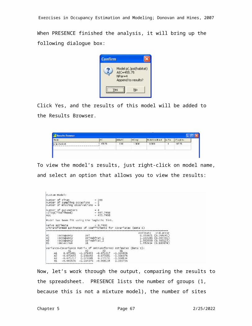
Exercises in Occupancy Estimation and Modeling; Donovan and Hines, 2007
Before running this model, we need to initialize the DM. Start off by writing out the logit equations:Logit y = a1 *1 + a2 * habitat_1 + a3 * habitat_2Logit p1 = b1 * 1 + b2 * temp1 + b3 * rain1Logit p2 = b4 * 1 + b5 * temp2 + b6 * rain2 + b7 * recapture.
Remember, we only need to enter the recapture effect for p2 because p2 is a function of whether the species was detected on survey 1 or not. Go ahead and set up both the occupancy and detection equations. Here’s the DM we used for detection:
When you run this model, only run 100 bootstrap trials, and add the results to the Results Browser:
The results are the same as the spreadsheet, except that PRESENCE nicely orders them by AIC weight. Let’s take a look at the output:
Chapter 5 Page 67 5/9/2023
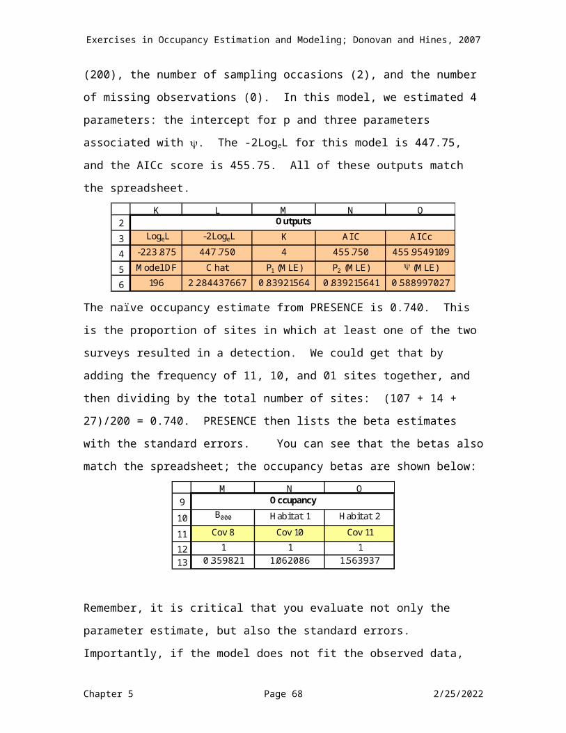
Exercises in Occupancy Estimation and Modeling; Donovan and Hines, 2007
9
10
11
1213
F G H I J K L M N O
B0 Temp Rain B00 Temp Rain Recapture B000 Habitat 1 Habitat 2Cov 1 Cov 2 Cov 3 Cov 4 Cov 5 Cov 6 Cov 7 Cov 8 Cov 10 Cov 11
1 1 1 1 1 1 1 1 1 11.374383 0.922653 -0.133354 1.162958 -1.061997 -0.077562 1.412877086 0.460443 1.363276 1.870516
OccupancySurvey 1 Survey 2
A nice feature in PRESENCE is that the betas (a1, a2, a3, b1, …b7) are labeled automatically, so you know which beta corresponds to which covariate.
Scroll down to the very bottom of the PRESENCE output to look at the Chi-Square results:
Remember, you must run a GOF test on at least one model in your model set. Otherwise, you’ll never know if you are just ranking a bunch of lousy models….at least one most must predict fairly well the site histories that you observed in the field. As you can see from the Model Fit results, the Chi-Square test statistic from this model is 5.2472. Well, does this indicate that the data fit or not? After simulating 100 different datasets based on the betas from this model,
Chapter 5 Page 68 5/9/2023

Exercises in Occupancy Estimation and Modeling; Donovan and Hines, 2007
and running the model and computing Chi-Square for each one, the results suggest that a Chi-Square value of 5.2472 falls within the 7.92 percentile of the bootstrap data. In other words, 7.9% of the bootstap chi-square values were higher than the observed value, and 100-7.9% = 92.1% of the bootstrap chi-square values were lower than the observed value. This is one of those values that is hard to interpret. If our probability was 0.03 instead of 0.079, we would conclude there is evidence of lack of fit. If our probability was 0.5 instead of 0.079, we would conclude there is no evidence of lack of fit. We’re in the grey zone. Fortunately, we don’t need to make an arbitrary decision. Lack of fit results in standard error estimates that are too low. If the data fit perfectly, c-hat is 1. In this analysis, c-hat is estimated at 2.228. PRESENCE computed that as the observed chi-square divided by the mean of the bootstrap chi-square values. Because this value is greater than 1, you should multiply each of your standard error estimates by the square root of c-hat. This applies to all standard errors in the entire model set. Under the ‘Tools’ menu, there’s a choice to change c-hat. This should change the ‘AIC’s to QAIC’s.
SUMMARYThat wraps up this exercise. In the remaining exercises, we will not be using the Design Matrix for modeling. Rather, we will simply focus on the concepts and mechanics behind the various model options in PRESENCE. However, in almost all cases, you’ll want to include either survey specific or site-level covariates. The methods you’ve used here to specify a model in the DM apply to any of the models in PRESENCE. Remember, write out your logit equations first; rows in the DM are where you specify the linear equation for a given parameter, while columns in the DM assign the beta and effects to that parameter.
Chapter 5 Page 69 5/9/2023


