Expectations, Learning and MacroeconomicPolicy

George W. Evans (University of Oregon and University of St.Andrews)

26 March 2010

J. C. Trichet: “Understanding expectations formation as a process underscoresthe strategic interdependence that exists between expectations formation andeconomics.” (Zolotas lecture, 2005)

Ben S. Bernanke: “In sum, many of the most interesting issues in contempo-rary monetary theory require an analytical framework that involves learning byprivate agents and possibly the central bank as well.” (NBER, July 2007).

Outline

Morning Session

Lecture 1: Review of techniques: E- stability & least squares learning– Muth model. Multivariate Models. Application to New Keynesian model

Lecture 2: Optimal monetary policy and learning– Optimal policy with learning. Policy with perpetual learning

Afternoon session

Lecture 3: (i) Recurrent hyperinflations and learning– (ii) Dynamic Predictor Selection and Endogenous Volatility

Lecture 4: Liquidity traps, learning and stagnation.

Lecture 1: Review of techniques: E- stability & least squareslearning

Introduction

• Since Lucas (1972, 1976) and Sargent (1973) the standard assumption inthe theory of economic policy is rational expectations (RE). This assumes,for both private agents and policymakers,

— knowledge of the correct form of the model

— knowledge of all parameters, and

— knowledge that other agents are rational & know that others know . . . .

• RE assumes too much and is therefore implausible. We need an appropriatemodel of bounded rationality What form should this take?

• My general answer is given by the Cognitive Consistency Principle: eco-nomic agents should be about as smart as (good) economists.Economists forecast economic variables using. econometric techniques, soa good starting point: model agents as “econometricians.”

• Neither private agents nor economists at central banks do know the truemodel. Instead economists formulate and estimate models. These modelsare re-estimated and possibly reformulated as new data becomes available.Economists engage in processes of learning about the economy.

• These processes of learning create new tasks for macroeconomic policy

Starting Points:

• The private sector is forward-looking (e.g. investment, savings decisions).

• Forecasts (including private forecasts) of future inflation and output havea key role in monetary policy:

1. Empirical evidence e.g. by (Clarida, Gali and Gertler 1998).

2. Bank of England and ECB discuss private forecasts in addition to in-ternal macro projections.

• Private agents and/or policy-makers are learning.

Fundamental Problems:

• There may be multiple equilibria, depending on interest rate policy.

• Policy may lead to expectational instability if expectations are not alwaysrational.

These problems necessitate careful design of interest rate rule: Bullard andMitra (2002), Evans and Honkapohja (2003a, 2006).=> Survey papers: Evans and Honkapohja (2003b, 2009), Bullard (2006).

• Central message: Policy should facilitate learning by private agents.

A Muth/Lucas-type Model

Before looking at issues of policy, we review the learning approach and theE-stability technique, beginning with a simple univariate reduced form:

pt = μ+ αE∗t−1pt + δ0wt−1 + ηt. (RF)

E∗t−1pt denotes expectations of pt formed at t− 1, wt−1 is a vector of exoge-nous shocks observed at t− 1, ηt is an exogenous unobserved iid shock, andwt follows an exogenous stationary VAR process.

Muth example. Demand and supply equations:

dt = mI −mppt + v1tst = rI + rpE

∗t−1pt + r0wwt−1 + v2t,

Assuming market clearing, st = dt, yields (RF) where μ = (mI − rI)/mp,δ = −m−1p rw and α = −rp/mp and ηt = (v1t − v2t)/mp.Note that α < 0 if mp, rp > 0.

Lucas-type Monetary model. A simple Lucas-type model:

qt = q + π(pt −E∗t−1pt) + ζt,

where π > 0, and aggregate demand function is given by

mt + vt = pt + qt,

vt = μ+ γ0wt−1 + ξt,

mt = m+ ut + ρ0wt−1.Here wt−1 are exogenous observables. The reduced form is again

pt = μ+ αE∗t−1pt + δ0wt−1 + ηt, where

α = π(1 + π)−1 and δ = (1 + π)−1(ρ+ γ)

In this example 0 < α < 1.

RATIONAL EXPECTATIONS

First consider the model under RE:

pt = μ+ αEt−1pt + δ0wt−1 + ηt.

The model has a unique RE solution since

Et−1pt = μ+ αEt−1pt + δ0wt−1 −→Et−1pt = (1− α)−1δ + (1− α)−1δ0wt−1

Hence the unique REE is

pt = a+ b0wt−1 + ηt, where

a = (1− α)−1δ and b = (1− α)−1δ.

LEAST-SQUARES LEARNING

Under learning, agents have the beliefs or perceived law of motion (PLM)

pt = a+ bwt−1 + ηt,

but a, b are unknown. At the end of time t−1 they estimate a, b by LS (LeastSquares) using data through t−1, i.e. Then they use the estimated coefficientsto make forecasts E∗t−1pt. Here the standard least squares (LS) formula areÃ

at−1bt−1

!=

⎛⎝t−1Xi=1

zi−1z0i−1

⎞⎠−1⎛⎝t−1Xi=1

zi−1pi

⎞⎠ , where

z0i =³1 w0i

´.

The timing is:

— End of t− 1: wt−1 and pt−1 observed. Agents update estimates of a, b toat−1, bt−1 using {ps, ws−1}t−1s=1. Agents make forecasts

E∗t−1pt = at−1 + b0t−1wt−1.

— Period t: (i) The shock ηt is realized, pt is determined as

pt = (μ+ αat−1) + (δ + αbt−1)0wt−1 + ηt

and wt is realized. (ii) agents update estimates to at, bt using {ps, ws−1}ts=1and make forecasts

E∗t pt+1 = at + b0twt.

The system under learning is a fully specified dynamic system under learning.

Question: Will (at, bt)→ (a, b) as t→∞?

LS updating and the system can be set up recursively. Letting

φt =

Ãatbt

!and zt =

Ã1wt

!the system is:

E∗t−1pt = at−1 + b0t−1wt−1pt = μ+ αE∗t−1pt + δ0wt−1 + ηt,

φt = φt−1 + t−1R−1t zt−1(pt − φ0t−1zt−1)Rt = Rt−1 + t−1(zt−1z0t−1 −Rt−1),

This recursive formulation is useful for (a) theoretical analysis, and (b) numer-ical simulations.

Theorem: Consider model (RF) with E∗t−1pt = at−1 + b0t−1wt−1 and with

at−1, bt−1 updated over time using least-squares. If α < 1 then

Ãatbt

!→Ã

ab

!with probability 1. If α > 1 convergence occurs with probability 0.

Thus the REE is stable under LS learning both for Muth model (α < 0) andLucas model (0 < α < 1)..

Example of an unstable REE: Muth model with mp < 0 (Giffen good) and|mp| < rp.

E-STABILITY

Proving the theorem is not easy. However, there is an easy way of deriving thestability condition α < 1 that is quite general. Start with the PLM

pt = a+ b0wt−1 + ηt,

and consider what would happen if (a, b) were fixed at some value possiblydifferent from the RE values (a, b). The corresponding expectations are

E∗t−1pt = a+ b0wt−1,which would lead to the Actual Law of Motion (ALM)

pt = μ+ α(a+ b0wt−1) + δ0wt−1 + ηt.

The implied ALM gives the mapping T : PLM → ALM:

T

Ãab

!=

Ãμ+ αaδ + αb

!.

The REE a, b is a fixed point of T . Expectational-stability (“E-stability) isdefined by the differential equation

d

dτ

Ãab

!= T

Ãab

!−Ãab

!.

Here τ denotes artificial or notional time. a, b is said to be E-stable if it isstable under this differential equation.

In the current case the T -map is linear. Component by component we have

da

dτ= μ+ (α− 1)a

dbidτ

= δ + (α− 1)bi for i = 1, ..., p.

da

dτ= μ+ (α− 1)a

dbidτ

= δ + (α− 1)bi for i = 1, ..., p.

It follows that the REE is E-stable if and only if α < 1. This is the stabilitycondition, given in the theorem, for stability under LS learning.

Intuition: under LS learning the parameters at, bt are slowly adjusted, on aver-age, in the direction of the corresponding ALM parameters.

Numerical simulation of learning in Muth model. μ = 5, δ = 1 and α = −0.5.wt

iid∼ N(0, 1) and ηtiid∼ N(0, 1/4). Initial values a0 = 1, b0 = 2 and

R0 = eye(2). Convergence to the REE a = 10/3 and b = 2/3 is rapid.

40 View of the Landscape

Figure 2.1.

A general definition of E-stability is a straightforward extension of the ex-ample in this chapter. Starting with an economic model, we consider its REEsolutions. Assume that any particular solution can be described as a stochasticprocess with particular parameter values φ. Here φ might be, for example, theparameters of an ARMA process or of a VAR or the mean values at the differ-ent points in a k-cycle. Under adaptive learning the agents are assumed not toknow φ, but try to estimate it using data from the economy. This leads to statisti-cal estimates φt at time t , and the issue will be whether φt → φ as t→∞. Wewill in each case set up the problem as an SRA in order to examine the stabilityof the solution φ. We will continue to find that stability of φ under learning canbe determined by the E-stability equation, i.e., by the stability of

dφ

dτ= T (φ)− φ, (2.20)

in a neighborhood of φ, where T (φ) is the mapping from the perceived lawof motion φ to the implied actual law of motion T (φ). [Note that REEs corre-

The E-Stability Principle

— The E-stability technique works quite generally.

— To study convergence of LS learning to an REE, specify a PLM with para-meters φ. The PLM can be thought of as an econometric forecasting model.The REE is the PLM with φ = φ.

— PLMs can take the form of ARMA or VARs or admit cycles or a dependenceon sunspots.

— Compute the ALM for this PLM. This gives a map

φ→ T (φ),

with fixed point φ.

— E-stability is determined by local asymptotic stability of φ under

dφ

dτ= T (φ)− φ.

The E-stability condition is that all eigenvalues of DT (φ) have real parts lessthan 1.

— The E-stability principle: E-stability governs local stability of an REE underLS and closely related learning rules.

— E-stability can be used as a selection criterion in models with multiple REE.

— These techniques can be applied to multivariate linearized models, and thusto RBC, OLG, New Keynesian and DSGE models.

The New Keynesian Model

• Log-linearized New Keynesian model (CGG 1999, Woodford 2003 etc.).

1. “IS” equation (IS curve)

xt = −ϕ(it −E∗t πt+1) +E∗t xt+1 + gt

2. the “New Phillips” equation (PC curve)

πt = λxt + βE∗t πt+1 + ut,

where xt =output gap, πt =inflation, it = nominal interest rate. E∗t xt+1,E∗t πt+1 are expectations. Parameters ϕ, λ > 0 and 0 < β < 1.

• Observable shocks followÃgtut

!= F

Ãgt−1ut−1

!+

Ãgtut

!, F =

Ãμ 00 ρ

!,

where 0 < |μ| , |ρ| < 1, and gt ∼ iid(0, σ2g), ut ∼ iid(0, σ2u).

• Interest rate setting by a standard Taylor rule, e.g.it = χππt + χxxt where χπ, χx > 0 orit = χππt−1 + χxxt−1 orit = χπE

∗t πt+1 + χxE

∗t xt+1

• Under learning we treat the IS and PC Euler equations as behavioral equa-tions. Explicit infinite-horizon formations also have been studied: Preston(IJCM, 2005 and JME, 2006), Evans, Honkapohja & Mitra (JME, 2009).For more on Euler equation learning see Evans and McGough (2009).

Determinacy and Stability under Learning

DETERMINACY

Combining IS, PC and the it rule leads to a bivariate reduced form in xt andπt.Letting y0t = (xt, πt)0 and v0t = (gt, ut)0 the model can be writtenÃ

xtπt

!=M

ÃE∗t xt+1E∗t πt+1

!+N

Ãxt−1πt−1

!+ P

Ãgtut

!,

yt =ME∗t yt+1 +Nyt−1 + Pvt.

If the model is “determinate” there exists a unique stationary REE of the form

yt = byt−1 + cvt.

Determinacy condition: compare # of stable eigenvalues of matrix of stackedfirst-order system to # of predetermined variables. If “indeterminate” there aremultiple solutions, which include stationary sunspot solutions.

LEARNING

Under learning, agents have beliefs or a perceived law of motion (PLM)

yt = a+ byt−1 + cvt,

where we now allow for an intercept, and estimate (at, bt, ct) in period t basedon past data.

- Forecasts are computed from the estimated PLM.- New data is generated according to the model with the given forecasts.- Estimates are updated to (at+1, bt+1, ct+1) using least squares.

Question: when is it the case that

(at, bt, ct)→ (0, b, c)?

We determine this using E-stability

E-STABILITY

Reduced form

yt =ME∗t yt+1 +Nyt−1 + Pvt.

Under the PLM (Perceived Law of Motion)

yt = a+ byt−1 + cvt.

E∗t yt+1 = (I + b)a+ b2yt−1 + (bc+ cF )vt.

This −→ ALM (Actual Law of Motion)

yt =M(I + b)a+ (Mb2 +N)yt−1 + (Mbc+NcF + P )vt.

This gives a mapping from PLM to ALM:

T (a, b, c) = (M(I + b)a,Mb2 +N,Mbc+NcF + P ).

The optimal REE is a fixed point of T (a, b, c). If

d/dτ(a, b, c) = T (a, b, c)− (a, b, c)is locally asymptotically stable at the REE it is said to be E-stable. See EH,Chapter 10, for details. The E-stability conditions can be stated in terms ofthe derivative matrices

DTa = M(I + b)

DTb = b0 ⊗M + I ⊗Mb

DTc = F 0 ⊗M + I ⊗Mb,

where ⊗ denotes the Kronecker product and b denotes the REE value of b.

E-stability governs stability under LS learning.

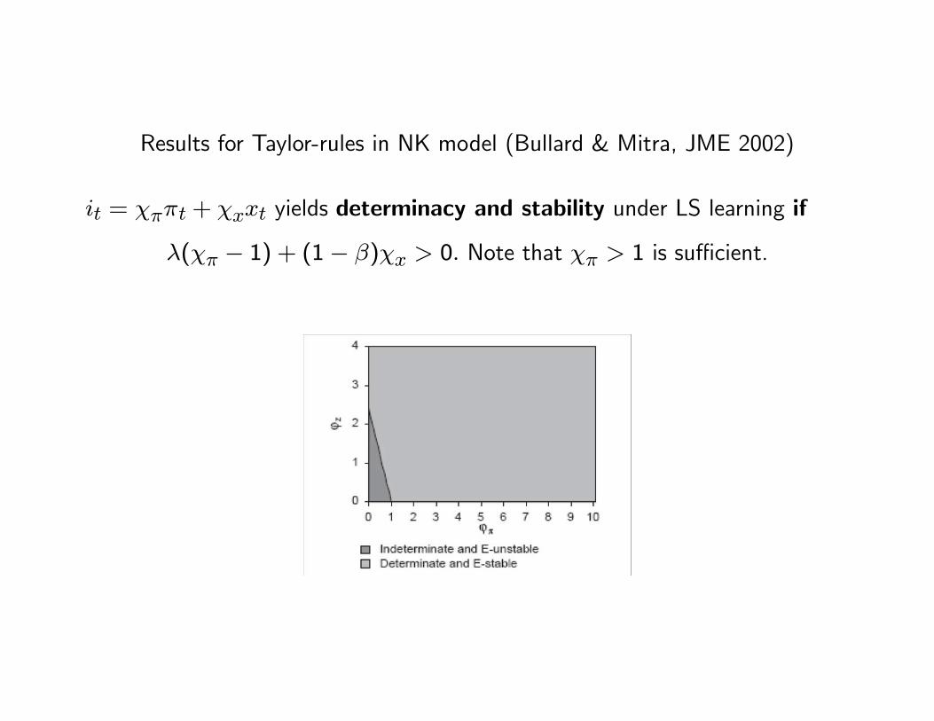
Results for Taylor-rules in NK model (Bullard & Mitra, JME 2002)

it = χππt + χxxt yields determinacy and stability under LS learning if

λ(χπ − 1) + (1− β)χx > 0. Note that χπ > 1 is sufficient.

With it = χππt−1 + χxxt−1, determinacy & E-stability for χπ > 1 andχx > 0 small. Also an explosive region (χπ > 1 and χx large) and adeterminate E-unstable region (χπ < 1 and χx moderate).

For it = χπE∗t πt+1+χxE

∗t xt+1, determinacy & E-stability for χπ > 1 and

χx > 0 small. Indeterminate & E-stable for χπ > 1 and χx large. Recentwork has shown stable sunspot solutions in that region.