23
Expected accuracy sequence alignment Usman Roshan
| Date post: | 20-Dec-2015 |
| Category: |
Documents |
| View: | 226 times |
| Download: | 1 times |

Expected accuracy sequence alignment
Usman Roshan

Optimal pairwise alignment
• Sum of pairs (SP) optimization: find the alignment of two sequences that maximizes the similarity score given an arbitrary cost matrix. We can find the optimal alignment in O(mn) time and space using the Needleman-Wunsch algorithm.
• Recursion: Traceback:
€
€
M(i, j) =
M(i −1, j −1) + s(x i, y j )
M(i, j −1) + g
M(i −1, j) + g
⎧
⎨ ⎪
⎩ ⎪
where M(i,j) is the score of the optimal alignment of x1..i and y1..j, s(xi,yj) is a substitution scoring matrix, and g is the gap penalty
Affine gap penalties
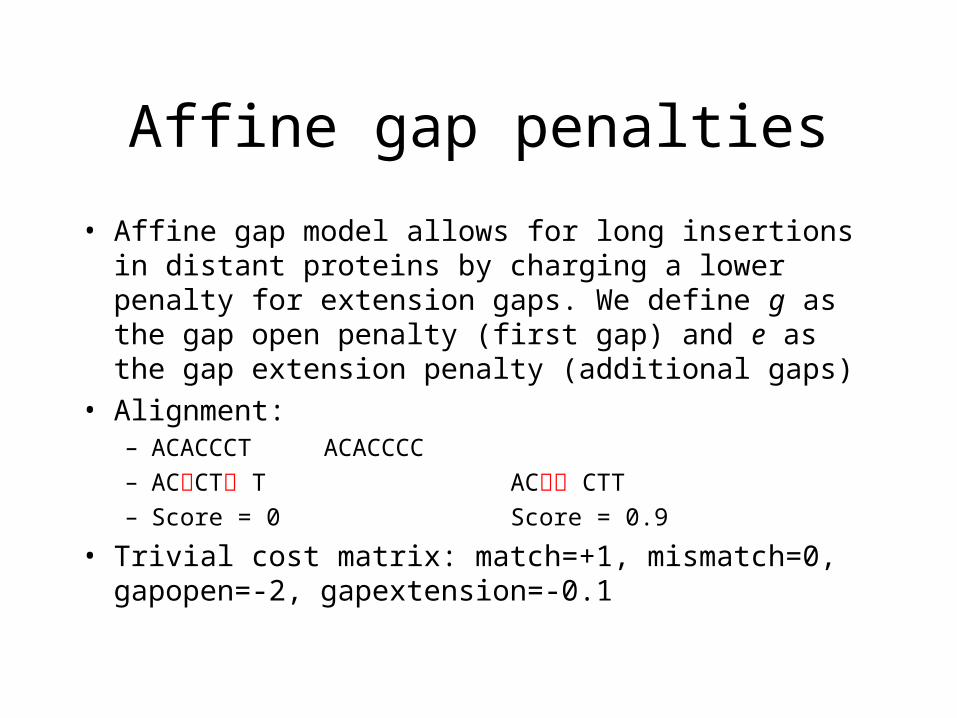
• Affine gap model allows for long insertions in distant proteins by charging a lower penalty for extension gaps. We define g as the gap open penalty (first gap) and e as the gap extension penalty (additional gaps)
• Alignment:– ACACCCT ACACCCC– ACCT T AC CTT– Score = 0 Score = 0.9
• Trivial cost matrix: match=+1, mismatch=0, gapopen=-2, gapextension=-0.1
Affine penalty recursion
€
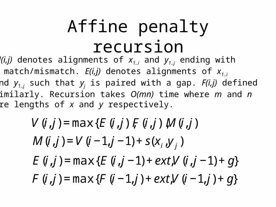
V (i, j) = max{E(i, j),F(i, j), M(i, j)
M(i, j) = V (i −1, j −1) + s(x i,y j )
E(i, j) = max{E(i, j −1) + ext,V (i, j −1) + g}
F(i, j) = max{F(i −1, j) + ext,V (i −1, j) + g}
M(i,j) denotes alignments of x1..i and y1..j ending witha match/mismatch. E(i,j) denotes alignments of x1..i
and y1..j such that yj is paired with a gap. F(i,j) definedsimilarly. Recursion takes O(mn) time where m and n are lengths of x and y respectively.
Expected accuracy alignment
• The dynamic programming formulation allows us to find the optimal alignment defined by a scoring matrix and gap penalties. This may not necessarily be the most “accurate” or biologically informative.
• We now look at a different formulation of alignment that allows us to compute the most accurate one instead of the optimal one.
Posterior probability of xi aligned to yj
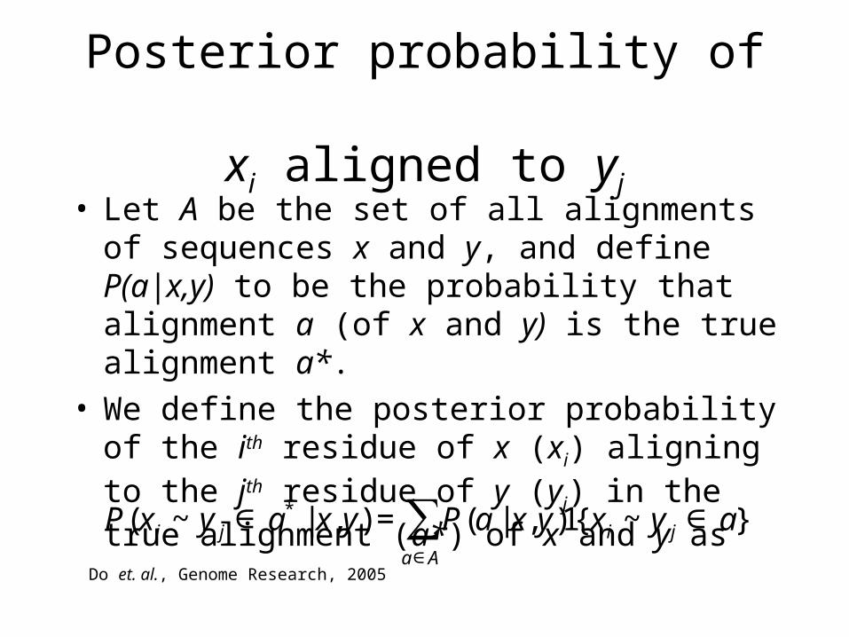
• Let A be the set of all alignments of sequences x and y, and define P(a|x,y) to be the probability that alignment a (of x and y) is the true alignment a*.
• We define the posterior probability of the ith residue of x (xi) aligning to the jth residue of y (yj) in the true alignment (a*) of x and y as
Do et. al., Genome Research, 2005
€
P(x i ~ y j ∈ a* | x,y) = P(a | x,y)1{x i ~ y j ∈ a}a∈A
∑

Expected accuracy of alignment
• We can define the expected accuracy of an alignment a as
• The maximum expected accuracy alignment can be obtained by the same dynamic programming algorithm
V i j
V i j P x y
V i j
V i j
i j
( , ) max
( , ) ( ~ )
( , )
( , )
=− − +
−−
⎧
⎨⎪
⎩⎪
⎫
⎬⎪
⎭⎪
1 111
Do et. al., Genome Research, 2005

Example for expected accuracy
• True alignment• AC_CG• ACCCA• Expected accuracy=(1+1+0+1+1)/4=1
• Estimated alignment• ACC_G• ACCCA• Expected accuracy=(1+1+0.1+0+1) ~ 0.75

Estimating posterior probabilities• If correct posterior probabilities can be computed
then we can compute the correct alignment. Now it remains to estimate these probabilities from the data
• PROBCONS (Do et. al., Genome Research 2006): estimate probabilities from pairwise HMMs using forward and backward recursions (as defined in Durbin et. al. 1998)
• Probalign (Roshan and Livesay, Bioinformatics 2006): estimate probabilities using partition function dynamic programming matrices

Partition function posterior probabilities
• Standard alignment score:
• Probability of alignment (Miyazawa, Prot. Eng. 1995)
• If we knew the alignment partition function then
SaT Mff gappenaltiesij i jija() ln( / )( _ )(,)= +∈∑Pa eSaT() ()/∝PaTe ZTSaT(,) /()()/=

Partition function posterior probabilities
• Alignment partition function (Miyazawa, Prot. Eng. 1995)
• SubsequentlyZ e e eijM SaTaA
S aTaA
sxyTijij
i ii j
i j, ()/ ()/ (, )/,= =⎛⎝⎜⎜ ⎞⎠⎟⎟∈ ∈∑ ∑−−−−
1111
€
Z(T) = eS(a ) /T
a∈A
∑

Partition function posterior probabilities
• More generally the forward partition function matrices are calculated as
Z Z Z Z eZZe ZeZZe ZeZZZZijM i jM i jE i jF sxyTijE ijMgT ijEextTijF i jMgT i jFextTij ijMijE ijF
i j, , . , (, )/, , / . /, , / . /, , , ,
( )=+ += += +=++−− −− −−− −− −11 11 111 11 1
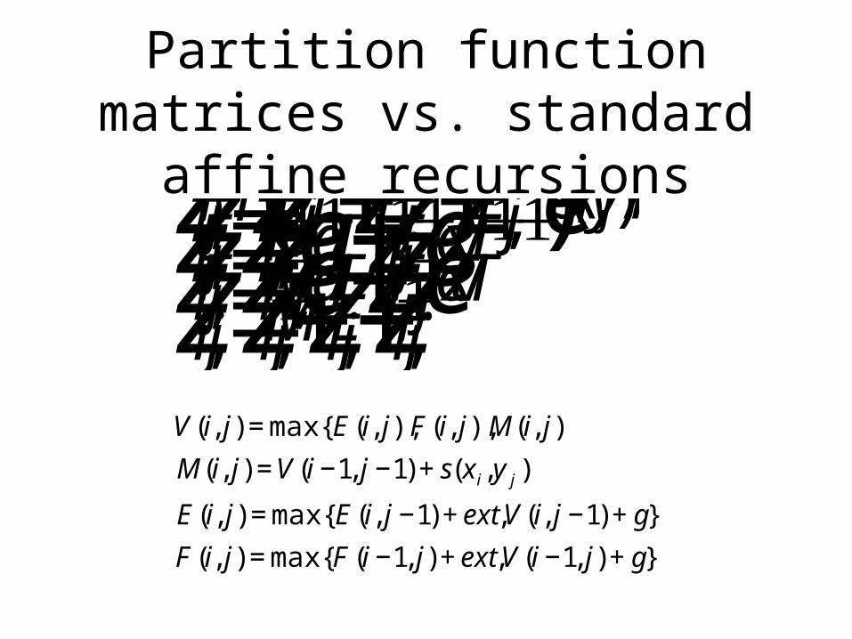
Partition function matrices vs. standard affine recursionsZ Z Z Z eZZe ZeZZe ZeZZZZijM i jM i jE i jF sxyTijE ijMgT ijEextTijF i jMgT i jFextTij ijMijE ijF
i j, , . , (, )/, , / . /, , / . /, , , ,
( )=+ += += +=++−− −− −−− −− −11 11 111 11 1
€
V (i, j) = max{E(i, j),F(i, j),M(i, j)
M(i, j) = V (i −1, j −1) + s(x i,y j )
E(i, j) = max{E(i, j −1) + ext,V (i, j −1) + g}
F(i, j) = max{F(i −1, j) + ext,V (i −1, j) + g}
Posterior probability calculation
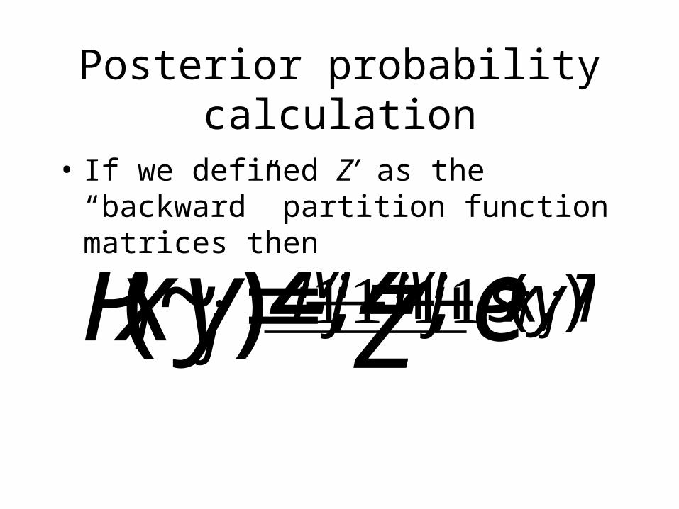
• If we defined Z’ as the “backward” partition function matrices then
Pxy Z ZZ ei j i jM i jM sxyTi j(~) ', , (, )/=−−++11 11

Posterior probabilities using alignment ensembles
• By generating an ensemble A(n,x,y) of n alignments of x and y we can estimate P(xi~yj) by counting the number of times xi is aligned to yj.. Note that this means we are assigning equal weights to all alignments in the ensemble.
€
P(x i ~ y j ∈ a* | x,y) = P(a | x,y)1{x i ~ y j ∈ a}a∈A
∑

Generating ensemble of alignments
• We can use stochastic backtracking (Muckstein et. al., Bioinformatics, 2002) to generate a given number of optimal and suboptimal alignments.
• At every step in the traceback we assign a probability to each of the three possible positions.
• This allows us to “sample” alignments from their partition function probability distribution.
• Posteror probabilities turn out to be the same when calculated using forward and backward partition function matrices.

Probalign1. For each pair of sequences (x,y) in the input set
– a. Compute partition function matrices Z(T)– b. Estimate posterior probability matrix P(xi ~ yj) for (x,y)
by
2. Perform the probabilistic consistency transformation and compute a maximal expected accuracy multiple alignment: align sequence profiles along a guide-tree and follow by iterative refinement (Do et. al.).
Pxy Z ZZ ei j i jM i jM sxyTi j(~) ', , (, )/=−−++11 11
V i j
V i j P x y
V i j
V i j
i j
( , ) max
( , ) ( ~ )
( , )
( , )
=− − +
−−
⎧
⎨⎪
⎩⎪
⎫
⎬⎪
⎭⎪
1 111
Multiple protein alignment
• Protein sequence alignment: hard problem for multiple distantly related proteins
• Several standard protein alignment benchmarks available: BAliBASE, HOMSTRAD, OXBENCH, PREFAB, and SABMARK
• Benchmark alignments are based on manual and computational structural alignment of proteins with known structure.

Measure of accuracy
• Sum-of-pairs score: number of correctly aligned pairs divided by number of pairs in true alignment.
• Column score: number of correctly aligned columns
• Statistical significance using Friedman rank test
AACAGTAAGT_ _
AACAGTAA_ _GT
Blue: correctRed: incorrectAcc: 2/4=50%

Experimental design
• Methods compared:– Probalign– PROBCONS– MUSCLE– MAFFT
• Probalign temperature parameter trained on RV11 subset of BAliBASE 3.0.
• Default (optimized) parameters for remaining programs
• All experiments performed on CIPRES cluster at SDSC

BAliBASE 3.0
Data Probalign MAFFT Probcons MUSCLE
RV11 69.3 / 45.3 67.1 / 44.6 67.0 / 41.7 59.3 / 35.9
RV12 94.6 / 86.2 93.6 / 83.8 94.1 / 85.5 91.7 / 80.4
RV20 92.6 / 43.9 92.7 / 45.3 91.7 / 40.6 89.2 / 35.1
RV30 85.2 / 56.4 85.6 / 56.9 84.5 / 54.4 80.3 / 38.3
RV40 92.2 / 60.3 92.0 / 59.7 90.3 / 53.2 86.7 / 47.1
RV50 89.3 / 55.2 90.0 / 56.2 89.4 / 57.3 85.7 / 48.7
All 87.6 / 58.9 87.1 / 58.6 86.4 / 55.8 82.5 / 48.5
Method RV11 RV12 RV20 RV30 RV40 RV50 All
MAFFT NS < 0.005 NS NS < 0.005 NS < 0.005
Probcons 0.049 0.0233 NS NS < 0.005 NS < 0.005
MUSCLE < 0.005 < 0.005 0.008 < 0.005 < 0.005 NS < 0.005
Sum-of-pairs and column score accuracies
Friedman rank test P-values

Heterogeneous length data I
Max length /Standard dev.
Probalign MAFFT Probcons MUSCLE
500 / 100 88.4 / 56.6 88.0 / 58.0 86.7 / 51.6 81.5 / 42.5
500 / 200 88.5 / 54.6 87.0 / 51.9 87.2 / 48.9 81.9 / 42.4
1000 / 100 91.4 / 58.1 90.4 / 55.7 89.7 / 51.6 84.3 / 44.1
1000 / 200 90.7 / 55.0 89.3 / 51.4 89.2 / 48.7 83.2 / 42.5
RV40 1000 / 100 (25) 1000 / 200 (20)
92.7 / 59.393.0 / 57.3
91.0 / 54.890.8 / 52.1
89.9 / 48.290.6 / 47.6
BAliBASE datasets with maximum length and minimum devation
BAliBASE datasets with long extensions
Max length /Standard dev.
Probalign MAFFT Probcons

Heterogeneous length data II
Max length /Standard dev.
Probalign MAFFT Probcons
500 / 100 (40) 89.1 / 44.9 87.3 / 49.0 87.4 / 38.6
500 / 200 (21) 88.3 / 43.8 85.0 / 46.4 86.7 / 40.0
500 / 300 (9) 95.3 / 61.0 82.6 / 51.3 87.3 / 46.6
500 / 400 (5) 94.6 / 55.0 72.0 / 38.2 79.8 / 38.0
1000 / 100 (15) 90.2 / 43.3 82.4 / 36.9 85.4 / 27.6
1000 / 200 (12) 89.2 / 38.2 79.7 / 32.4 83.6 / 27.7
1000 / 300 (7) 94.5 / 52.8 78.3 / 42.4 83.9 / 34.6
1000 / 400 (5) 94.6 / 55.0 72.0 / 38.2 79.8 / 38.0
BAliBASE 2.0 reference 6 datasets with max length and minimum deviation


