Experience With Subcycle Operating Time Distance Elements in Transmission

Line Digital Relays

Gabriel Benmouyal and Karl Zimmerman Schweitzer Engineering Laboratories, Inc.

Presented at the 37th Annual Western Protective Relay Conference

Spokane, Washington October 19–21, 2010

1

Experience With Subcycle Operating Time Distance Elements in Transmission Line Digital Relays

Gabriel Benmouyal and Karl Zimmerman, Schweitzer Engineering Laboratories, Inc.

Abstract—The first experimental digital transmission line relays were designed with simple and primitive filtering systems that offered, at least theoretically, an operating time of a few milliseconds. Very rapidly, protection engineers realized the relationship between a filter data window and protection element security. The short window turned out to be impractical and unreliable, and designers resorted to full-cycle Fourier or cosine filters in the early and subsequent commercial digital transmission line relays. Following the technological maturity and general acceptance reached by these relays with a nominal response close to 1 cycle, the need to achieve subcycle operating times arose about 15 years ago.

The purpose of this paper is to revisit the basic issues determining the speed of a transmission line relay and review the various techniques introduced to achieve faster operating speeds. Operations of relays installed in the field are presented and analyzed.

I. INTRODUCTION Full-cycle Fourier and cosine phasor filtering systems have

become the de facto standard for the implementation of numerical transmission line protection functions. This state-of-the-art technology was not reached overnight but was the result of a compromise. This solution was the outcome of a long process, at the end of which protection engineers realized that there was a relation between a filter data window length and its security: the longer the data window, the more secure and slower the filter. In early experimental numerical line transmission relays where filter data windows could have a few samples [1] [2], fast operating times were achieved at the expense of reliability and security. One of the first experimental digital line transmission relays boasted operation times close to a half cycle [1]. Historically, filters with a data window length of 1 cycle have allowed reasonable operating speed together with security and reliability [3]. The solid-state technology that preceded the numerical era was successful in producing transmission line relays with subcycle operating times. This was achievable because the solid-state comparators used for the implementation of distance elements did not require numerical filters for the computation of signal phasors. Rather, they made use of the time waveforms of voltages and currents at their inputs so that fast operating times could be achieved with little implemented filtering.

In the early 1980s, a new brand of relays called ultra-high-speed (UHS) directional relays was introduced by relay manufacturers [4]. These units were advertised with operating times close to 0.25 cycle. Used in directional comparison schemes, the units achieved subcycle operating times, particularly on series-compensated transmission lines.

Based on the operating speed achieved by some solid-state relays, the performance of UHS directional relays, and the operating times imposed by stability criteria on some power networks, requirements for faster or subcycle numerical distance elements emerged within the protection industry in the mid-1990s.

The purpose of this paper is to review the technical challenges encountered with the design of very fast numerical distance elements, revisit the possible solutions, and analyze and evaluate the performance of relays installed in the field.

II. DISTANCE ELEMENT BASIC REQUIREMENTS

A. Implementation of Mho Elements In a transmission line relay, each of six impedance loops

has to be covered by a distance element corresponding to the three phase-to-ground fault loops (AG, BG, and CG) and the three phase-to-phase fault loops (AB, BC, and CA).

Covering an impedance loop with a mho characteristic requires defining one operating vector and one polarizing vector, as shown in (1).

op

pol pol

S r • ZL1• Ir – Vr

S V

=

= (1)

where: r is the element reach. ZL1 is the line positive-sequence impedance. Ir is the current at the input of the element. Vr is the voltage at the input of the element.

The most popular polarization method is the use of the positive-sequence voltage memory (V1M).

The element asserts when the scalar product (P) between the operating quantity and the polarizing quantity is positive or when it satisfies the inequality in (2).

( ) ( )polP real r • ZL • Ir – Vr • conj V 0⎡ ⎤= ≥⎣ ⎦ (2)

where: real represents “real part of.” conj stands for “conjugate of.”

The scalar product is tantamount to implementing an angle comparator: if the angle between the polarizing quantity and the operating quantity becomes smaller than 90 degrees, the element asserts.

2

An alternate solution to the scalar product in (2) is to calculate the distance to the fault m, as shown in (3), and then compare the calculated m value to some reach threshold [5].

pol

pol

real [Vr • conj (V )]m

real [ZL • Ir • conj (V )]= (3)

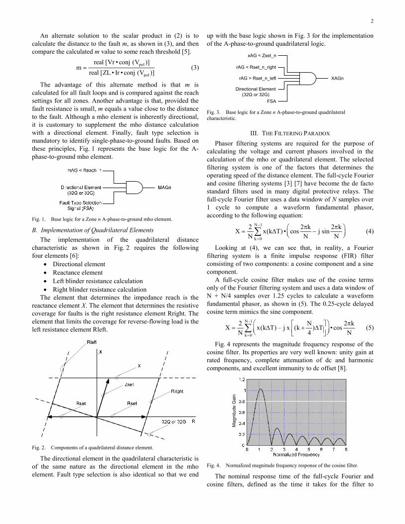
The advantage of this alternate method is that m is calculated for all fault loops and is compared against the reach settings for all zones. Another advantage is that, provided the fault resistance is small, m equals a value close to the distance to the fault. Although a mho element is inherently directional, it is customary to supplement the mho distance calculation with a directional element. Finally, fault type selection is mandatory to identify single-phase-to-ground faults. Based on these principles, Fig. 1 represents the base logic for the A-phase-to-ground mho element.

Fig. 1. Base logic for a Zone n A-phase-to-ground mho element.

B. Implementation of Quadrilateral Elements The implementation of the quadrilateral distance

characteristic as shown in Fig. 2 requires the following four elements [6]:

• Directional element • Reactance element • Left blinder resistance calculation • Right blinder resistance calculation

The element that determines the impedance reach is the reactance element X. The element that determines the resistive coverage for faults is the right resistance element Rright. The element that limits the coverage for reverse-flowing load is the left resistance element Rleft.

Fig. 2. Components of a quadrilateral distance element.

The directional element in the quadrilateral characteristic is of the same nature as the directional element in the mho element. Fault type selection is also identical so that we end

up with the base logic shown in Fig. 3 for the implementation of the A-phase-to-ground quadrilateral logic.

xAG < Zset_n

rAG < Rset_n_right

rAG > Rset_n_left

Directional Element (32Q or 32G)

FSA

XAGn

Fig. 3. Base logic for a Zone n A-phase-to-ground quadrilateral characteristic.

III. THE FILTERING PARADOX Phasor filtering systems are required for the purpose of

calculating the voltage and current phasors involved in the calculation of the mho or quadrilateral element. The selected filtering system is one of the factors that determines the operating speed of the distance element. The full-cycle Fourier and cosine filtering systems [3] [7] have become the de facto standard filters used in many digital protective relays. The full-cycle Fourier filter uses a data window of N samples over 1 cycle to compute a waveform fundamental phasor, according to the following equation:

N–1

k 0

2 2 k 2 kX x(k T) • cos j sin

N N N=

π π⎛ ⎞= Δ −⎜ ⎟⎝ ⎠∑ (4)

Looking at (4), we can see that, in reality, a Fourier filtering system is a finite impulse response (FIR) filter consisting of two components: a cosine component and a sine component.

A full-cycle cosine filter makes use of the cosine terms only of the Fourier filtering system and uses a data window of N + N/4 samples over 1.25 cycles to calculate a waveform fundamental phasor, as shown in (5). The 0.25-cycle delayed cosine term mimics the sine component.

N –1

k 0

2 N 2 kX x(k T) – j x (k ) T • cos

N 4 N=

⎛ ⎞ π⎡ ⎤= Δ + Δ⎜ ⎟⎢ ⎥⎝ ⎠⎣ ⎦∑ (5)

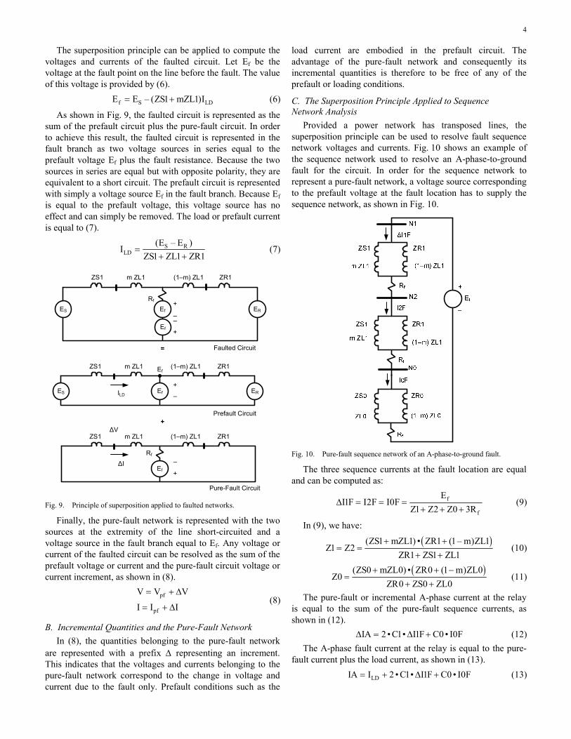
Fig. 4 represents the magnitude frequency response of the cosine filter. Its properties are very well known: unity gain at rated frequency, complete attenuation of dc and harmonic components, and excellent immunity to dc offset [8].

Mag

nitu

de G

ain

Fig. 4. Normalized magnitude frequency response of the cosine filter.

The nominal response time of the full-cycle Fourier and cosine filters, defined as the time it takes for the filter to

3

measure the magnitude of a voltage or current step function, is equal to the time interval of the data window: respectively 1 cycle or 16.66 milliseconds for the Fourier filter and 1.25 cycles or 20.82 milliseconds for the cosine filter at 60 Hz.

Assuming a relay has fast tripping output contacts, the fault detection time of a distance element in a numerical relay depends essentially upon the nature of the filtering system used for the calculation of the voltage and current phasors and the system conditions. The most favorable system conditions in terms of the relay speed are as follows:

• A system with a low source impedance ratio (SIR) • A fault close to the substation • A fault with low resistance

Obviously, these conditions correspond to a fault with a high fault current and maximum voltage depression.

The most adverse system conditions in terms of the relay speed are simply the opposite of the most favorable conditions:

• A system with a high SIR • A fault remote from the substation • A fault with high resistance

These conditions lead to a fault with a small change both in the current and voltage of the phase (or phases).

When implementing a distance element using full-cycle filters, the relay detection time is below the filter nominal response time, typically around 0.75 cycle in the most favorable conditions and possibly beyond 2 cycles in the most adverse conditions. The average operating time is therefore slightly more than 1 cycle.

Notwithstanding the system conditions, it is obvious that full-cycle conventional filters are inadequate for the purpose of implementing high-speed or subcycle operating time distance elements. We have to resort to filtering systems with a shorter data window. Fig. 5 represents the magnitude frequency response of the two components of the Fourier filter with a data window of a half cycle.

1.4

1.21

0.8

0.6

0.4

0.2

00 60 120

Frequency (Hz)180 240 300 360 420 480

Cosine Component

Sine Component

Fig. 5. Half-cycle data window Fourier dual-component filter magnitude frequency response.

Comparing the two plots in Fig. 5 with the full-cycle cosine filter frequency response in Fig. 4, we can see that as we increase the filter data window, the filtering system becomes more immune to dc and off-nominal frequency components. The half-cycle data window Fourier filter rejects odd harmonics but is still not immune to dc components.

As the data window of a Fourier filter becomes smaller, the filtering system becomes more impacted by dc offset components as they exist in faulty current waveforms [8]. If we use a Fourier filtering system, there is an obligation to use a mimic filter [8] or some other means to mitigate the impact of the dc offset in the current waveforms. This mimic filter adds a small time delay to the Fourier filter response.

Fig. 6 shows the magnitude frequency response of each of the two components of the half-cycle window Fourier system combined with a mimic filter. Fig. 7 shows the magnitude response to a fully offset unit step function of the half-cycle Fourier filter with and without the addition of a mimic filter [8]. Without the mimic filter, the magnitude presents an overshoot of more than 80 percent, whereas with the mimic filter, the overshoot is reduced to a mere 4 percent.

2

1.5

1

0.5

00 60 120Frequency (Hz)

Filte

r Gai

n

Sine Component

Cosine Component

180 240 300 360 420 480

Fig. 6. Combined mimic half-cycle Fourier dual-component filter magnitude frequency response.

Mag

nitu

de O

utpu

t

Fig. 7. Impact of a mimic filter in the magnitude acquisition of a fully offset current wave.

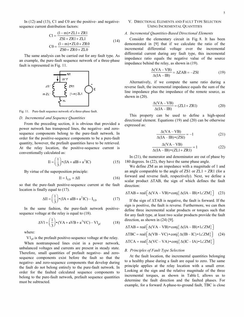
IV. THE VIRTUES OF THE PURE-FAULT NETWORK

A. The Superposition Principle Applied to Power Network Faults

Before addressing the issue of high-speed directional and fault type selection elements, we revisit the nature of the pure-fault network.

Consider the elementary power network in Fig. 8, and assume a fault occurs at a distance m in per-unit value from the left bus.

L R

ZS1ZS0

ZR1ZR0

ZL1ZL0

m

ES ER

Fig. 8. Elementary power system network.

4

The superposition principle can be applied to compute the voltages and currents of the faulted circuit. Let Ef be the voltage at the fault point on the line before the fault. The value of this voltage is provided by (6). f S LDE E – (ZS1 mZL1)I= + (6)

As shown in Fig. 9, the faulted circuit is represented as the sum of the prefault circuit plus the pure-fault circuit. In order to achieve this result, the faulted circuit is represented in the fault branch as two voltage sources in series equal to the prefault voltage Ef plus the fault resistance. Because the two sources in series are equal but with opposite polarity, they are equivalent to a short circuit. The prefault circuit is represented with simply a voltage source Ef in the fault branch. Because Ef is equal to the prefault voltage, this voltage source has no effect and can simply be removed. The load or prefault current is equal to (7).

S RLD

(E – E )I

ZS1 ZL1 ZR1=

+ + (7)

ZS1 ZR1m ZL1 (1–m) ZL1

Rf

Faulted Circuit

ZS1 ZR1m ZL1 (1–m) ZL1

Prefault Circuit

ZS1 ZR1m ZL1 (1–m) ZL1

Rf

Pure-Fault Circuit

ILD

Ef

ES

=

+

ER

Ef

Ef

Ef

Ef

+

––

+

+

–

+–

ΔV

ΔI

ES ER

Fig. 9. Principle of superposition applied to faulted networks.

Finally, the pure-fault network is represented with the two sources at the extremity of the line short-circuited and a voltage source in the fault branch equal to Ef. Any voltage or current of the faulted circuit can be resolved as the sum of the prefault voltage or current and the pure-fault circuit voltage or current increment, as shown in (8).

pf

pf

V V V

I I I

= + Δ

= + Δ (8)

B. Incremental Quantities and the Pure-Fault Network In (8), the quantities belonging to the pure-fault network

are represented with a prefix Δ representing an increment. This indicates that the voltages and currents belonging to the pure-fault network correspond to the change in voltage and current due to the fault only. Prefault conditions such as the

load current are embodied in the prefault circuit. The advantage of the pure-fault network and consequently its incremental quantities is therefore to be free of any of the prefault or loading conditions.

C. The Superposition Principle Applied to Sequence Network Analysis

Provided a power network has transposed lines, the superposition principle can be used to resolve fault sequence network voltages and currents. Fig. 10 shows an example of the sequence network used to resolve an A-phase-to-ground fault for the circuit. In order for the sequence network to represent a pure-fault network, a voltage source corresponding to the prefault voltage at the fault location has to supply the sequence network, as shown in Fig. 10.

Fig. 10. Pure-fault sequence network of an A-phase-to-ground fault.

The three sequence currents at the fault location are equal and can be computed as:

f

f

EI1F I2F I0F

Z1 Z2 Z0 3RΔ = = =

+ + + (9)

In (9), we have:

( )(ZS1 mZL1) • ZR1 (1– m)ZL1

Z1 Z2ZR1 ZS1 ZL1

+ += =

+ + (10)

( )(ZS0 mZL0) • ZR0 (1 m)ZL0

Z0ZR0 ZS0 ZL0

+ + −=

+ + (11)

The pure-fault or incremental A-phase current at the relay is equal to the sum of the pure-fault sequence currents, as shown in (12). IA 2 • C1• I1F C0 • I0FΔ = Δ + (12)

The A-phase fault current at the relay is equal to the pure-fault current plus the load current, as shown in (13). LDIA I 2 • C1• I1F C0 • I0F= + Δ + (13)

5

In (12) and (13), C1 and C0 are the positive- and negative-sequence current distribution factors:

(1 m) • ZL1 ZR1C1

ZS1 ZR1 ZL1(1 m) • ZL0 ZR0

C0ZS0 ZR0 ZL0

− +=

+ +− +

=+ +

(14)

The same analysis can be carried out for any fault type. As an example, the pure-fault sequence network of a three-phase fault is represented in Fig. 11.

Fig. 11. Pure-fault sequence network of a three-phase fault.

D. Incremental and Sequence Quantities From the preceding section, it is obvious that provided a

power network has transposed lines, the negative- and zero-sequence components belong to the pure-fault network. In order for the positive-sequence components to be a pure-fault quantity, however, the prefault quantities have to be retrieved. At the relay location, the positive-sequence current is conventionally calculated as:

21I1 • (IA aIB a IC)

3⎛ ⎞= + +⎜ ⎟⎝ ⎠

(15)

By virtue of the superposition principle: LDI1 I I1= + Δ (16)

so that the pure-fault positive-sequence current at the fault location is finally equal to (17).

2LD

1I1 • (IA aIB a IC) – I

3⎛ ⎞Δ = + +⎜ ⎟⎝ ⎠

(17)

In the same fashion, the pure-fault network positive-sequence voltage at the relay is equal to (18).

2pf

1V1 • (VA aVB a VC) – V1

3⎛ ⎞Δ = + +⎜ ⎟⎝ ⎠

(18)

where: V1pf is the prefault positive-sequence voltage at the relay.

When nontransposed lines exist in a power network, unbalanced voltages and currents are present in steady state. Therefore, small quantities of prefault negative- and zero-sequence components exist before the fault so that the negative- and zero-sequence components that develop during the fault do not belong entirely to the pure-fault network. In order for the faulted calculated sequence components to belong to the pure-fault network, prefault sequence quantities must be subtracted.

V. DIRECTIONAL ELEMENTS AND FAULT TYPE SELECTION USING INCREMENTAL QUANTITIES

A. Incremental Quantities-Based Directional Elements Consider the elementary circuit in Fig. 8. It has been

demonstrated in [9] that if we calculate the ratio of the incremental differential voltage over the incremental differential current during any fault type, this incremental impedance ratio equals the negative value of the source impedance behind the relay, as shown in (19).

(VA – VB)

ZAB –ZS1(IA – IB)

Δ= Δ =

Δ (19)

Alternatively, if we compute the same ratio during a reverse fault, the incremental impedance equals the sum of the line impedance plus the impedance of the remote source, as shown in (20).

(VA – VB)

(ZL1 ZR1)(IA – IB)

Δ= +

Δ (20)

This property can be used to define a high-speed directional element. Equations (19) and (20) can be otherwise expressed as:

(VA – VB)

–1(IA – IB) • (ZS1)Δ

=Δ

(21)

(VA – VB)

1(IA – IB) • (ZL1 ZR1)

Δ=

Δ + (22)

In (21), the numerator and denominator are out of phase by 180 degrees. In (22), they have the same phase angle.

We define ZM as an impedance with a magnitude of 1 and an angle comparable to the angle of ZS1 or ZL1 + ZR1 (for a forward and reverse fault, respectively). Next, we define a scalar product ∆TAB, the sign of which defines the fault direction:

TAB real (VA – VB) • conj (IA – IB) •1 ZMΔ = ⎡Δ Δ ∠ ⎤⎣ ⎦ (23)

If the sign of ΔTAB is negative, the fault is forward. If the sign is positive, the fault is reverse. Furthermore, we can then define three incremental scalar products or torques such that for any fault type, at least two scalar products provide the fault direction, as shown in (24) [9].

TAB real (VA – VB) • conj (IA – IB) •1 ZM

TBC real (VB – VC) • conj (IB – IC) •1 ZM

TCA real (VC – VA) • conj (IC – IA) •1 ZM

Δ = ⎡Δ Δ ∠ ⎤⎣ ⎦Δ = ⎡Δ Δ ∠ ⎤⎣ ⎦Δ = ⎡Δ Δ ∠ ⎤⎣ ⎦

(24)

B. Principles of Fault Type Selection At the fault location, the incremental quantities belonging

to a healthy phase during a fault are equal to zero. The same principle applies at the relay location with a small error. Looking at the sign and the relative magnitude of the three incremental torques, as shown in Table I, allows us to determine the fault direction and the faulted phases. For example, for a forward A-phase-to-ground fault, TBC is close

6

to zero when TAB and TCA have about the same value and are negative. Based on these principles, we generate 14 logic signals from the incremental quantities. These signals provide direction and fault type selection, as shown in Table II [9] [10]. This function is called high-speed directional and fault type selection (HSD-FTS).

TABLE I RELATIVE VALUES OF INCREMENTAL TORQUES

Fault Type TAB TBC TCA

AG TAB 0 TAB

BG TAB TAB 0

CG 0 TBC TBC

AB, ABG TAB 0.25 • TAB 0.25 • TAB

BC, BCG 0.25 • TBC TBC 0.25 • TBC

CA, CAG 0.25 • TCA 0.25 • TCA TCA

ABC TAB TAB TAB

TABLE II HIGH-SPEED DIRECTIONAL SIGNALS

Logic Signals Fault Type and Direction

HSD-AGF, HSD-AGR Forward, reverse A-phase-to-ground fault

HSD-BGF, HSD-BGR Forward, reverse B-phase-to-ground fault

HSD-CGF, HSD-CGR Forward, reverse C-phase-to-ground fault

HSD-ABF, HSD-ABR Forward, reverse A-to-B-phase fault

HSD-BCF, HSD-BCR Forward, reverse B-to-C-phase fault

HSD-CAF, HSD-CAR Forward, reverse C-to-A-phase fault

HSD-ABCF, HSD-ABCR Forward, reverse A-to-B-to-C-phase fault

C. Comparison With Conventional Sequence Quantities-Based Directional Elements

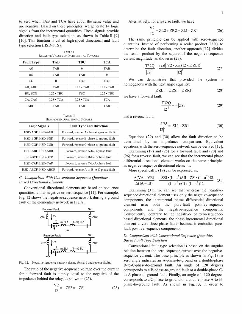
Conventional directional elements are based on sequence quantities, either negative or zero sequence [11]. For example, Fig. 12 shows the negative-sequence network during a ground fault of the elementary network in Fig. 8.

m ZL1 (1–m) ZL1

N2

ZS2 ZR2V2

I2

m ZL1 (1–m) ZL1

N2

ZS2 ZR2V2

I2

Forward Fault

Reverse Fault

Fig. 12. Negative-sequence network during forward and reverse faults.

The ratio of the negative-sequence voltage over the current for a forward fault is simply equal to the negative of the impedance behind the relay, as shown in (25).

V2

–ZS2 –ZS1I2

= = (25)

Alternatively, for a reverse fault, we have:

V2

ZL2 ZR2 ZL1 ZR1I2

= + = + (26)

The same principle can be applied with zero-sequence quantities. Instead of performing a scalar product T32Q to determine the fault direction, another approach [12] divides the scalar product by the square of the negative-sequence current magnitude, as shown in (27).

[ ]

2 2

real V2 • conj(I2 •1 ZL1)T32Q

I2 I2

∠= (27)

We can demonstrate that provided the system is homogenous with the next angle equality: ZL1 ZS1 ZR1∠ = ∠ = ∠ (28) we have a forward fault:

2

T32Q– ZS1

I2= (29)

and a reverse fault:

2

T32QZL1 ZR1

I2= + (30)

Equations (29) and (30) allow the fault direction to be determined by an impedance comparison. Equivalent equations with the zero-sequence network can be derived [12].

Examining (19) and (25) for a forward fault and (20) and (26) for a reverse fault, we can see that the incremental phase differential directional element works on the same principles as negative-sequence directional elements.

More specifically, (19) can be expressed as:

2 2

2 2

(VA – VB) –ZS1• (1– a ) I1 ZS1• (1– a )I2(IA – IB) (1– a ) I1 (1 a )I2

Δ Δ −=

Δ Δ + − (31)

Examining (31), we can see that whereas the negative-sequence directional element uses only the negative-sequence components, the incremental phase differential directional element uses both the pure-fault positive-sequence components and the negative-sequence components. Consequently, contrary to the negative- or zero-sequence-based directional elements, the phase incremental directional element covers three-phase faults because it embodies pure-fault positive-sequence components.

D. Comparison With Conventional Sequence Quantities-Based Fault Type Selection

Conventional fault type selection is based on the angular relation between the zero-sequence current over the negative-sequence current. The base principle is shown in Fig. 13: a zero angle indicates an A-phase-to-ground or a double-phase B-to-C-phase-to-ground fault. An angle of 120 degrees corresponds to a B-phase-to-ground fault or a double-phase C-to-A-phase-to-ground fault. Finally, an angle of –120 degrees corresponds to a C-phase-to-ground or a double-phase A-to-B-phase-to-ground fault. As shown in Fig. 13, in order to

7

account for various factors, a tolerance of ±30 degrees is introduced to determine the faulted phase.

FSA

FSB

FSC

120°

30°

30°

–120°

Fig. 13. Angular relation between I0 over I2.

We can conclude at this stage that fault type selection based on incremental phase differential components has some differences with respect to conventional fault type selection based on the angle between I0 and I2. Namely, the differences are:

• Fault type selection based on incremental phase differential components uses both the voltage and current incremental components.

• Fault type selection based on incremental phase differential components uses the relative levels of three incremental torques that provide the fault direction.

E. Advantages of Incremental Quantities

1) Load-Independent Performance Because incremental quantities belong to the pure-fault

network, they are automatically free of any load effect that could affect the directional element.

2) Cancellation of Nontransposition Effects As already noted, due to the presence of nontransposed

lines, small quantities of sequence components can exist before the fault. When computing incremental quantities, any component existing before the fault is removed so that the incremental quantities components can be considered as belonging entirely to the pure-fault network.

3) Extremely Fast Response Time Incremental quantities-based directional elements using

single-phase components can be created as well. For a forward A-phase-to-ground fault, we have:

–(2 • C1• ZS1 C0 • ZS0)VA

ZAIA 2• C1 C0

+Δ= Δ =

Δ + (32)

Alternatively, for a reverse fault, we have:

(2 • C1• ZS1 C0 • ZS0)VA

ZAIA 2 • C1 C0

+Δ= Δ =

Δ + (33)

In both (32) and (33), C1 and C0 are close to a real number (the imaginary part is very small). For a forward fault, we end up with an incremental impedance that is negative and highly inductive. For a reverse fault, we end up with an incremental impedance that is positive and highly inductive. If we use the same unity mimic as before (ZM), a scalar product can be defined as:

TA real (VA) • conj (IA) •1 ZM= ⎡Δ Δ ∠ ⎤⎣ ⎦ (34)

This scalar product is equal to: TA VA • IA • cos= Δ Δ θ (35)

In (35), θ is the angle between the two incremental phasors. θ is a small angle to account for the error in the angle of ZM that cannot exactly match the angle of one of the two impedances it is supposed to mimic. In the worst-case scenario, θ should be an angle of a few degrees.

The same scalar product can be performed in the time domain. We assume that the time equations of the A-phase incremental voltage and current after the inception of the fault are provided by (36) for a forward fault.

va(t) va • sin( t )ia(t) – ia • sin( t )

Δ = Δ ω + ψΔ = Δ ω + ψ + θ

(36)

In (36), Δia(t) is the incremental current, the angle of which is advanced by an angle equal to that of the mimic. We can then perform the following integration immediately after the inception of the fault:

T

0T

0

2Ta(t) va(t) • ia (t) • dt

T

2 va •sin( t) • – ia • sin( t ) • dtT

= Δ Δ =

Δ ω Δ ω + ψ + θ

∫

∫ (37)

so that we have at the end of one period T for a forward fault: Ta(T) – va • ia • cos= Δ Δ θ (38)

For a reverse fault, we have the same value but with an appositive sign: Ta(T) va • ia • cos= Δ Δ θ (39)

When performing the integration in (37), it is not necessary to wait a full period T to get the result of the scalar product. A few samples after the integration is started, the integral sign reaches either positive or negative territory and the fault direction is determined. Theoretically, the direction can be determined almost instantaneously. This basic principle is the one on which UHS directional relays designed in the early 1980s were based [4]. Practically, the operating time turns out to be a few milliseconds after some security counts are implemented in order to overcome the noise and noxious frequency components, such as traveling waves present in the signals immediately following the fault inception.

8

VI. THE DERIVATION OF INCREMENTAL QUANTITIES

A. The Primitive Delta Filter In order to extract incremental quantities components, early

applications made use of delta filters in their simplest form, the principle of which is represented in Fig. 14.

–Tse

Fig. 14. Simple delta filter.

As shown in Fig. 14, the original delta filter was applied to time waveforms and simply subtracted from a signal at rated frequency (voltage or current) the same signal delayed by a time equal to 1 cycle. The delayed signal that is subtracted becomes the reference signal. The outcome of this operation is that, during a time equal to the delay T, the delta filter restitutes the time waveform corresponding to the change in voltage or current due to a network event. If this event is a fault, the delta filter output corresponds to the incremental voltage or current due to the fault over a period of time equal to the set delay.

B. More Advanced Delta Filters When deriving incremental quantities from phasors rather

than time waveforms, we can design more advanced delta filters that are more in tune with the superposition theorem. Fig. 15 shows the basic logic of a latching memory delta filter. This design requires an event detector that can simply monitor the changes in one or more incremental quantities. When a change is detected corresponding to a new event on the network, the reference signal value is latched to a memory register. At the same time, switch S2 toggles to the bottom position and provides as its output an incremental quantity, the reference value of which is a fixed phasor corresponding to the pre-event variable value. The incremental quantity is available during a time interval equal to the dropout time D1 of the timer.

–Tse

Fig. 15. Latching memory delta filter.

C. Shortcomings of Incremental Quantities

1) Lack of Signals During Switch-Onto-Fault Situation When a line is open and the line breaker is switched on an

existing fault, measured prefault conditions are zero and do not correspond to the real prefault network values. Therefore, during a switch-onto-fault situation, proper incremental quantities are not available.

2) Incremental Quantities During Cascading Events When applying the superposition principle as represented

in Fig. 9, it is necessary to define a new prefault network every time a change occurs on the power system. Practically, during a cascade of events that may occur over a short time period, the nature of the delta filter is such that the succession of changes could become intractable. One solution to this issue is to block the delta filters for a few cycles after a fault is detected. This provision is not applicable to evolving faults because the prefault conditions do not change in this situation.

VII. PRACTICAL IMPLEMENTATION OF HIGH-SPEED DISTANCE ELEMENTS

A. Mho Element Applications The base mho detector logic, as shown in Fig. 1, is

normally implemented using voltage and current phasors that have been processed through a standard filter such as the full-cycle cosine filtering system.

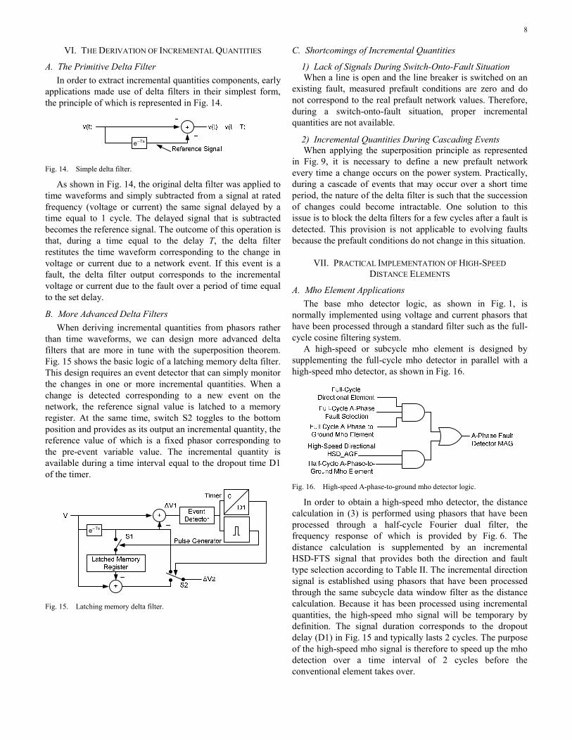
A high-speed or subcycle mho element is designed by supplementing the full-cycle mho detector in parallel with a high-speed mho detector, as shown in Fig. 16.

Fig. 16. High-speed A-phase-to-ground mho detector logic.

In order to obtain a high-speed mho detector, the distance calculation in (3) is performed using phasors that have been processed through a half-cycle Fourier dual filter, the frequency response of which is provided by Fig. 6. The distance calculation is supplemented by an incremental HSD-FTS signal that provides both the direction and fault type selection according to Table II. The incremental direction signal is established using phasors that have been processed through the same subcycle data window filter as the distance calculation. Because it has been processed using incremental quantities, the high-speed mho signal will be temporary by definition. The signal duration corresponds to the dropout delay (D1) in Fig. 15 and typically lasts 2 cycles. The purpose of the high-speed mho signal is therefore to speed up the mho detection over a time interval of 2 cycles before the conventional element takes over.

9

B. High-Speed Mho Element Simulation Results Fig. 17 represents an elementary 500 kV power system

with a 200-kilometer transmission line simulated in the Electromagnetic Transients Program (EMTP). Impedance values are in Ω primary. For this system, Fig. 18 represents the mho logic signals for an A-phase-to-ground fault at Bus L staged at 100 milliseconds. The HSD_AGF signal is extremely fast and responds in 3 milliseconds. The Zone 1 high-speed mho element (MAG1H) responds in 5 milliseconds. The conventional forward ground directional element (F32G) responds in 4 milliseconds and is almost as fast as the high-speed element. The conventional fault type selection signal (FSA) responds in 7 milliseconds, and finally, the conventional Zone 1 mho element (MAG1F) responds in 11 milliseconds.

∠∠

∠∠

∠∠

∠

Fig. 17. Example of a long line.

Fig. 18. Zone 1 mho logic signals for an A-phase-to-ground fault at the left substation.

Fig. 19 represents the combined mho element logic when the same fault is applied at 33 percent of the line. The high-speed mho detection time increased to 9 milliseconds, whereas the conventional mho element detection time increased to 1 cycle. Fig. 20 represents the trajectories of the distance m calculation using the half-cycle and full-cycle filter phasors.

Fig. 19. Zone 1 mho logic signals for an A-phase-to-ground fault at 33 percent of the line length seen from the left substation.

1.5

1

0.5

0

Dis

tanc

e m

(pu)

Time (s)0.1 0.11 0.12 0.13 0.14 0.15

2

Zone 2 Reach

Zone 1 Reach

High-Speed m Calculation

Conventional m Calculation

Fig. 20. High-speed and conventional distance m calculation for an A-phase-to-ground fault at 33 percent of the line length.

C. Quadrilateral Element Applications Exactly the same approach as for the mho elements can be

taken for the design of a high-speed quadrilateral distance characteristic [6].

VIII. THE JUSTIFICATION FOR SUBCYCLE DISTANCE ELEMENTS

Power system faults and disturbances cause oscillations in the relative positions of machine rotors that result in power flow swings. The difference between a stable (return to a new equilibrium state) and unstable (loss of synchronism between groups of generators) swing is directly affected by the fault-clearing speed. Subcycle distance elements, along with the use of faster breakers, improve the likelihood of preserving power system stability during these conditions [7].

Subcycle distance elements also reduce the duration of through faults on transformers, which, in turn, reduces accumulated mechanical damage and extends transformer life [13].

Faster fault clearing can also improve power quality by reducing the duration of voltage sags [14].

IX. NETWORK CONDITIONS AFFECTING THE SPEED OF DISTANCE-BASED TRANSMISSION LINE RELAYS

The most influential network condition affecting the speed of distance-based elements is the SIR of the system. The SIR is defined as the ratio of the source behind the relay divided by the reach setting.

S

L

ZSIR

r • Z= (40)

As shown in Fig. 21, for a given reach setting, the stronger the source (smaller ZS) behind the relay, the faster the distance relays operate. The weaker the source (larger ZS), the slower the distance relay elements operate. Short (smaller ZL) lines tend to have a higher SIR.

r • ZL

ZL

VR

ZR

21

VS

ZS

Fig. 21. SIR based on source impedance (ZS) divided by reach setting, r • ZL.

10

X. EXAMPLE OF RELAY OPERATIONS FOR CONVENTIONAL LINES

This example relates to the operation of an A-phase-to-ground fault on a 75.8-kilometer 345 kV transmission line, as shown in Fig. 22.

∠∠

Fig. 22. A 345 kV conventional transmission line.

Fig. 23 shows the waveforms as captured by the event report at Substation L. Fig. 24 shows the distance m dual calculation as provided by the two filtering systems at the same substation. Fig. 25 shows the distance element logic signals at Substation L.

-1000

0

1000

-250

0

250

2.5 5.0 7.5 10.0 12.5 15.0

IA(A

) IB

(A) I

C(A

)V

A(k

V) V

B(k

V) V

C(k

V)

Cycles

IA(A) IB(A) IC(A) VA(kV) VB(kV) VC(kV)

Fig. 23. Event report waveforms at Substation L.

1.5

1

0.5

0

Dis

tanc

e m

(pu)

Time (s)0.09 0.1 0.11 0.12 0.13 0.14 0.15

2 High-Speed m Calculation

Conventional m Calculation

Zone 2 Reach

Zone 1 Reach

Fig. 24. A-phase-to-ground impedance loop distance m calculation.

Fig. 25. Zone 1 and Zone 2 A-phase-to-ground mho logic signals for a fault at about 10 percent of the line length from the substation.

The fault inception time at Substation L is 0.095 milliseconds. The HSD-FTS signal (HSD_AGF) asserts 4 milliseconds later. The high-speed Zone 1 mho element (MAG1H) asserts 14 milliseconds after the fault inception, whereas the high-speed Zone 2 mho signal (MAG2H) asserts 12 milliseconds after the fault inception. The conventional Zone 1 and Zone 2 mho signals (MAG1F and MAG2F) assert 10 milliseconds after the high-speed signals.

Fig. 26 shows the waveforms as captured by the event report at Substation R. Fig. 27 shows the distance m dual calculation as provided by the two filtering systems at Substation R. Fig. 28 shows the distance element logic signals at Substation L.

-2000

-1000

0

1000

2000

-200

-100

0

100

200

2.5 5.0 7.5 10.0 12.5 15.0

IA(A

) IB

(A) I

C(A

)V

A(k

V) V

B(k

V) V

C(k

V)

Cycles

IA(A) IB(A) IC(A) VA(kV) VB(kV) VC(kV)

Fig. 26. Event report waveforms at Substation R.

Dis

tanc

e m

(pu)

Fig. 27. A-phase-to-ground impedance loop distance m calculation.

Fig. 28. Zone 1 and Zone 2 A-phase-to-ground mho logic signals for a fault at about 90 percent of the line length from the substation.

The fault inception time at Substation R is 0.090 seconds. The HSD-FTS signal (HSD_AGF) asserts 2 milliseconds later. The high-speed Zone 2 mho signal (MAG2H) asserts 8 milliseconds after the fault inception. The conventional

11

Zone 2 mho signals (MAG2F) assert 12 milliseconds after the high-speed signal.

It should be noted that the communications-assisted permissive overreaching transfer trip (POTT) scheme benefits from the high-speed operation of the Zone 2 mho elements and provides subcycle or close to 1-cycle total operation time, depending upon the communications delays.

XI. EXAMPLE OF RELAY OPERATIONS FOR SERIES-COMPENSATED LINES

This example applies to a C-phase-to-ground fault occurring on a 277.15-kilometer 500 kV series-compensated line with 50 percent compensation in the middle of the line, as shown in Fig. 29.

∠∠

Fig. 29. Series-compensated transmission line.

The line is basically protected by a POTT scheme where the Zone 2 reach of the mho elements (phase and ground) is adjusted to 177 percent of the line length. The Zone 1 reach of the mho elements (phase and ground) is set to 26.6 percent of the line length. Fig. 30 shows the voltage and current waveforms as provided by the event report at Substation L.

-2500

0

2500

-250

0

250

2.5 5.0 7.5 10.0 12.5 15.0

IA(A

) IB

(A) I

C(A

)V

A(k

V) V

B(k

V) V

C(k

V)

Cycles

IA(A) IB(A) IC(A) VA(kV) VB(kV) VC(kV)

Fig. 30. Event report waveforms at Substation L.

Fig. 31 shows the distance element logic signals. The fault inception occurs at 0.095 seconds at Substation L. The Zone 2 high-speed mho fault detection occurs 10 milliseconds later when the conventional Zone 2 mho element adds up an additional delay of 10 milliseconds. Fig. 32 shows the distance m calculations as provided by the two filtering systems and the high-speed and conventional calculations.

Fig. 31. Zone 2 logic signals at Substation L.

Dis

tanc

e m

(pu)

Fig. 32. C-phase-to-ground impedance loop distance m calculations at Substation L.

Fig. 33 shows the voltage and current waveforms as provided by the event report at Substation R. Fig. 34 shows the distance element logic signals. The fault inception occurs at 0.1 seconds at Substation R. The Zone 2 high-speed mho fault detection occurs 10 milliseconds later, whereas the conventional Zone 2 mho element asserts with an additional delay of 10 milliseconds. Fig. 35 shows the distance m calculations as provided by the two filtering systems and the high-speed and conventional calculations.

The same as for the preceding example, with a conventional transmission line, high-speed Zone 2 distance elements used within the POTT communications scheme provide subcycle or close to 1-cycle total operation time, depending upon the communications delays.

-5000

-2500

0

2500

5000

-250

0

250

2.5 5.0 7.5 10.0 12.5 15.0

IA(A

) IB

(A) I

C(A

)V

A(k

V) V

B(k

V) V

C(k

V)

Cycles

IA(A) IB(A) IC(A) VA(kV) VB(kV) VC(kV)

Fig. 33. Event report waveforms at Substation R.

12

Fig. 34. Zone 2 logic signals at Substation R.

Dis

tanc

e m

(pu)

Fig. 35. C-phase-to-ground impedance loop distance m calculations at Substation R.

XII. CONCLUSIONS From the results presented in this paper, we conclude:

• Incremental phase or phase differential quantities allow the implementation of extremely fast directional elements free of load and network unbalance effects.

• Because incremental quantities belonging to healthy phases remain close to zero, fault type selection can be implemented in a straightforward fashion using the same quantities used for determining direction. Fault type selection then becomes as fast as the directional element.

• Contrary to directional elements based on negative- or zero-sequence components, incremental quantities applied to phase quantities allow the determination of direction for three-phase faults.

• The combination of subcycle distance calculations with high-speed directional and fault type selection elements allows supplementing conventional mho detectors and obtaining fast and reliable operation as demonstrated by numerous operations in the field.

XIII. REFERENCES [1] B. J. Mann and I. F. Morrison, “Relaying a Three-Phase Transmission

Line With a Digital Computer,” IEEE Transactions on Power Apparatus and Systems, Vol. PAS-90, Issue 2, March/April 1971.

[2] G. B. Gilchrist, G. D. Rockefeller, and E. A. Udren, “High-Speed Distance Relaying Using a Digital Computer, Part I,” IEEE Transactions on Power Apparatus and Systems, Vol. PAS-91, Issue 3, May/June 1972.

[3] E. O. Schweitzer, III and D. Hou, “Filtering for Protective Relays,” proceedings of the 19th Annual Western Protective Relay Conference, Spokane, WA, October 1992.

[4] M. Vitins, “A Fundamental Concept for High-Speed Relaying,” IEEE Transactions on Power Apparatus and Systems, Vol. PAS-100, Issue 1, January 1981.

[5] E. O. Schweitzer, III and J. Roberts, “Distance Relay Element Design,” proceedings of the 19th Annual Western Protective Relay Conference, Spokane, WA, October 1992.

[6] F. Calero, A. Guzmán, and G. Benmouyal, “Adaptive Phase and Ground Quadrilateral Distance Elements,” proceedings of the 36th Annual Western Protective Relay Conference, Spokane, WA, October 2009.

[7] H. J. Altuve Ferrer and E. O. Schweitzer, III (eds.), Modern Solutions for Protection, Control, and Monitoring of Electric Power Systems. Schweitzer Engineering Laboratories, Inc., Pullman, WA, 2010.

[8] G. Benmouyal, “Removal of DC-Offset in Current Waveform Using Digital Mimic Filtering,” IEEE Transactions on Power Apparatus and Systems, Vol. 10, Issue 2, April 1995.

[9] G. Benmouyal and J. Roberts, “Superimposed Quantities: Their True Nature and Their Application in Relays,” proceedings of the 26th Annual Western Protective Relay Conference, Spokane, WA, October 1999.

[10] A. Guzmán, J. Mooney, G. Benmouyal, and N. Fischer, “Transmission Line Protection System for Increasing Power System Requirements,” proceedings of the 55th Annual Conference for Protective Relay Engineers, College Station, TX, April 2002.

[11] J. Roberts and A. Guzmán, “Directional Element Design and Evaluation,” proceedings of the 21st Annual Western Protective Relay Conference, Spokane, WA, October 1994.

[12] A. Guzmán, J. Roberts, and D. Hou, “New Ground Directional Elements Operate Reliably for Changing System Conditions,” proceedings of the 51st Annual Georgia Tech Protective Relaying Conference, Atlanta, GA, April 1997.

[13] IEEE Guide for Liquid-Immersed Transformer Through-Fault-Current Duration, IEEE Standard C57.109-1993, May 1993.

[14] J. B. Roberts and K. Zimmerman, “Trip and Restore Distribution Circuits at Transmission Speeds,” proceedings of the 25th Annual Western Protective Relay Conference, Spokane, WA, October 1998.

XIV. BIOGRAPHIES Gabriel Benmouyal, P.E., received his BASc in electrical engineering and his MASc in control engineering from Ecole Polytechnique, Université de Montréal, Canada, in 1968 and 1970. In 1969, he joined Hydro-Québec as an instrumentation and control specialist. He worked on different projects in the fields of substation control systems and dispatching centers. In 1978, he joined IREQ, where his main fields of activity were the application of microprocessors and digital techniques for substations and generating station control and protection systems. In 1997, he joined Schweitzer Engineering Laboratories, Inc. as a principal research engineer. Gabriel is a registered professional engineer in the Province of Québec and an IEEE senior member and has served on the Power System Relaying Committee since May 1989. He holds over six patents and is the author or coauthor of several papers in the fields of signal processing and power network protection and control.

Karl Zimmerman is a senior power engineer with Schweitzer Engineering Laboratories, Inc. in Fairview Heights, Illinois. His work includes providing application and product support and technical training for protective relay users. He is an active member of the IEEE Power System Relaying Committee and chairman of the Working Group on Distance Element Response to Distorted Waveforms. Karl received his BSEE degree at the University of Illinois at Urbana-Champaign and has over 20 years of experience in the area of system protection. He is a past speaker at many technical conferences and has authored over 20 papers and application guides on protective relaying.

© 2010 by Schweitzer Engineering Laboratories, Inc. All rights reserved.

20100913 • TP6456-01