Experiences with Predicting Resource Performance On-line in Computational Grid Settings

Rich Wolski 12

A b s t r a c t

In this paper, we describe methods for predicting the perfor- mance of Computational Grid resources (machines, networks, storage systems, etc.) using computationally inexpensive sta- tistical techniques. The predictions generated in this man- ner are intended to support adaptive application scheduling in Grid settings, and on-line fault detection. Wedescrib e a mixture-of-experts approach to non-parametric, univariate time-series forecasting, and detail the effectiveness of the ap- proach using example data gathered from "production" (i.e. non-experimental) Computational Grid installations.

l i n t r o d u c t i o n

Performance prediction and evaluation are both critical components of the Computational Grid [12] architectural paradigm. In particular, predictions (especially those made at at run time) of available resource performance levels can be used to implement effective application scheduling [22, 24, 5, 25, 4]. Because Grid resources (the computers, networks, and storage systems that make up a Grid) differ widely in the per- formance they can deliver to any given application, and be- cause performance fluctuates dynamically due to contention by competing applications, schedulers (human or automatic) must be able to predict the deli~cerable performance that an ap- plication will be able to obtain when it eventually runs. Based on these predictions, the scheduler can choose the combina- tion of resources from the available resource pool that is ex- pected to maximize performance for the application.

Making the performance predictions that are necessary to sup- port scheduling typically requires a compositional model of application behavior which can be parameterized dynamically with resource information. For example, consider the prob- lem of selecting the machine from a Grid resource pool that delivers the fastest execution time for a sequential program. To choose from among a number of available target platforms, the scheduler must predict the execution speed of the applica- tion code on each of the platforms. Grid infrastructures such

tUniversity of California, Santa Barbara, Santa Barbara, California, 93106. email: rich@cs.ucsb.edu

2This work was supported, in large part, by grants from the National Science Foundation, numbered CAREER-0093166, EIA-9975020, ANI- 0213911, and ACI-9701333. In addition, the infrastructure development for public release that is discussed has been supported by the NSF National Part- nership for Advanced Computational Infrastructure (NPACI) and the NASA Information Power Grid project.

as Globus [ 11, 6] provide resource catalogs in which statically known attributes (such as CPU clock speed) are recorded. As such, the simplest approach to selecting the best machine is to query the catalog for all available hosts and then choose the one with the fastest clock rate.

There are several assumptions that underlie this simple ex- ample. One assumption is that the clock speeds of the vari- ous available CPUs can be used to rank the eventual execu- tion speeds of the program. Clock speed correlates well with execution performance if the machine pool is relatively ho- mogeneous. One of the basic tenets of the Grid paradigm, however, is that a wide variety of resource types are available. If, in this example, a floating point vector processor is avail- able, and the application vectorizes well, a slower clocked vector CPU could outperform a faster general purpose ma- chine making clock-speed an inaccurate predictor of applica- tion performance. Conversely,if it is a scalar integer code, a high-clock-rate vector machine might under-perform a slower commodity processor.

A second assumptioh is that the CPU is the only resource that needs to be considered as a parameter to the application model. If the input and output requirements for the program are substantial, the cost of reading the inputs and generating the outputs must also be considered. Generating estimates of the time required for the application to perform I/O is partic- ularly difficult in Grid settings since the I/O usually traverses a network. While static CPU attributes (e.g. clock speed) are typically recorded for Grid resources, network attributes and topology are not. Moreover, at the application level, the net- work performance estimates that are required are end-to-end. While it is possible to record the performance characteristics of various network components, composing those characteris- tics into a general end-to-end performance model has proved challenging [20,9 ,32,10,2 ,17,21] .

However, even if a model that effectively composes appli- cation performance from resource performance characteris- tics is available, the Grid resource pool cannot be assumed to be static. One of the key differentiating characteristics of Computational Grid computing is that the available resource pool can fluctuate dynamically. Resources are federated to the Grid by their resource owners who maintain ultimate lo- cal control. As such, resource owners may reclaim their re- sources, may upgrade or change the type and quantity of re- source that is available, etc. making "static" resource charac- teristics (e.g. the amount of memory supported by a machine)

41

potentially time-varying.

Even if resource availability is slowly changing, resource con- tention can cause the performance that can be delivered to any single application component to fluctuate with a much higher frequency.CPUs shared among several executing pro- cesses deliver only a fraction of their total capability to any one process. Network performance response is particularly dynamic. Most Grid systems, even if they use batch queues to provide unshared, dedicated CPU access to each applica- tion rely on shared networks for inter-machine communica- tion. The end-to-end network latency and throughput perfor- mance response can exhibit large variability, both in local area and wide area network settings. As such, the resource perfor- mance that will be available to the program (the fraction of each CPU's time slices, the network latency and throughput, the available memory) must be predicted for the time frame that the program will eventually execute.

Thus, to make a decision about where to run a sequential program given a pool of available machines from which to choose, a scheduler requires

• a performance model that correctly predicts (or ranks) execution performance when parameterized with re- source performance characteristics, and

* a method for estimating what the resource performance characteristics of the resources will be when the pro- gram executes.

In this paper, we focus on techniques for meeting the latter requirement. In particular, we discuss the use of statistical time-series analysis to make resource performance predic- tions from historically observed performance measurement data. We have used this methodology as part of the Network Weather Service (NWS) [31, 29, 19] - - a Grid middleware service that has been used extensively [22, 5, 28, 1,23, 30, 25, 4]to provide resource performance forecasts to Grid sched- ulers. We describe the specific techniques that have proved successful from our collaborations with various Grid schedul- ing projects, and we discuss various statistical features that we have observed while working with different Grid resources. This work is most closely related to the work of Dinda [7,8] who has studied the use of on-line time-series analysis mod- els for predicting host-load characteristics. Our approach dif- fers in its computational complexity and its ability to adapt to changing dynamics, but the goals are similar.

2The NWS Forecasting Methodology

The forecasting methodology used by the NWS assumes that each resource performance characteristic can be measured quantifiably. Each resource can be described by a stream of performance measurements, and predictions of future mea- surement values are the quantities that are of interest. Notice

that useful qualitative information may be difficult to incorpo- rate under this assumption. For example, it may be possible to know that "less" bandwidth will be available to a desktop machine which is; typically used by a person who frequently downloads images from the Internet than from a machine used by a person who typically works locally. The NWS approach is to gather performance measurements from both machines and then predict future measurement values so that the predic- tions can be compared quantitatively. For some Grid applica- tions, simply knowing "less" or "more" resource will be avail- able may be enough to develop an effective schedule. The ad- vantage of using quantifiable resource characterization, how- ever, is that the information is more easily encoded for use by an automatic scheduler. That is, it may be difficult for a scheduling agent to parse and compare the qualities of a re- source, but forecast quantities can almost always be compared if the units are compatible.

A second important assumption made by the NWS forecast- ing method is that performance measurements can be gath- ered non-intrusively. In particular, any load that the perfor- mance monitors introduce does not have a measurable effect on the resource being monitored.

Finally, because the methods are time series based, they as- sume that the characteristics being measured have an instan- taneous value that can be sampled at any given point in time. Not all quantifiable performance characteristics which are useful for scheduling easily conform to this model. For ex- ample, it is useful to predict the duration of time that a re- source will be available based on previous availability history. Availability, in a time series form, is a series of binary values indicating available or unavailable at a particular time. Thus, the measurement levels are bimodal. While Markov-based models are adept at predicting modality, time-series analysis tends to be less effective. It is possible to incorporate state- transition models into the NWS forecasting framework, but at present they are not used by the system.

Dynamic Model Differentiation Rather than relying on a single model, the NWS uses a mixture-of-experts approach to forecasting. A set of forecast- ing models are configured into the system, each having its own parameterization. Given a performance history of previ- ously observed measurement values, each model is exercised to generate a forecast for every measurement value based only on the measurement values that come before it. That is, given a performance history of N values, a forecast is generated for each. To generate a forecast for measurement k, only values up to measurement k - 1 will be presented to each forecast- ing model, for all values 1 < k < N. We term this method of replaying a performance history to generate a forecast for each known measurement value postcasting.

Postcast errors are generated for each forecasting method by differencing each measurement with the forecast generated for it. By aggregating the posteast errors, each method is as- signed an overall accuracy score for the complete history up to

42

the point in time when the forecast is generated. When a sin- gle forecast is required, the NWS forecasting system applies the postcasting procedure to all of the configured prediction models using the most recent performance history available, and ranks each prediction model in terms of its accuracy. The most accurate model is then chosen to make the requested forecast. Each time a forecast is requested, the NWS recal- culates the accuracy ranking using the most recently gathered history. The NWS constantly gathers measurement data from sensors that it controls. Thus, the performance histories that it uses are, typically, up-to-date at the time a forecast is re- quested from the system, and the forecaster choice takes into account the "fresh" historical data.

This method of differentiating between competing models based on previously observed accuracy has several advan- tages. The first is that it is non-parametric. Each individual model may have a specific parameterization, but the complete technique simply takes the constantly-updated performance history gathered by the NWS as its only input. A second po- tential advantage is that it is possible for the system to adapt to changing conditions in the cases where the performance response series is non-stationary. For example, if an expo- nential smoothing predictor with a gain factor of 0.01 is the most accurate predictor at one point in time, and conditions change so that a sliding window median predictor with a win- dow size of 10 becomes the most accurate (due to a change in the series dynamics) the system will switch predictors if the change is persistent enough to cause the aggregate error rank- ing to change. If, however, the forecasters have been exposed to an extensive performance history before the change point, it may take a great deal of time for the better method to garner a lower aggregate error.

To improve the response of the overall technique to changes in the underlying dynamics of each measurement series, the NWS forecasting subsystem also selectively limits the amount of history during postcasting to determine if "old" data is harming accuracy. During the dynamic model selec- tion phase, a postcast is conducted using all previously avail- able data. In addition, the system conducts postcasts using different windows of previous data (always starting with the most recent data and working backwards in time) and records the "winning" forecaster for each window size. The num- ber of postcast limiting windows and their sizes are fixed at compile time, but can be changed via configuration parame- ters when the forecasting subsystem is built. Each window size of previous history is subsequently treated as a separate forecaster and a final accuracy tournament determines which forecaster will be used.

The pseudocode shown in Figure 1 summarizes how NWS forecasts are generated from a given measurement trace. The effect of using this method is that either the forecaster that has the lowest aggregate error since the beginning of the trace will be chosen, or the forecaster that has the lowest error over an abbreviated history of fixed size will be chosen that the best forecaster. If the system has quickly changing dynamics,

input: T: measurement trace F: set of forecasting models that take a trace of fixed size and produce

a forecast of next value W: a set of integer window sizes to limit postcastln9

for each window size in W + (entire history) for each forecaster in F

postcast current forecaster over current window slze in T (window size slides over all of T)

record agsresate error for current forecaster end for record forecaster with lowest aggregate error for this window size

end for

choose forecaster and window size with lowest aggregated error and make final forecast using it

Figure 1: Pseudocode for NWS Forecasting Methodology

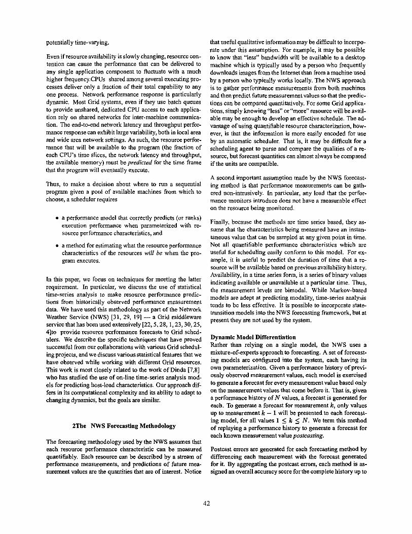
UTK to UCSD NWS Measured TCP/IP Throughput

June 1 through July 1, 2000

l - i i . ................. . ; - / . i . . . . . . ..................... i, ................................ ............................. i i i

,°,ililllllllfli/mtM o l ~''~1~ '1"" I ~,lll,~)" i ii I'"!

Figure 2: Internet Throughput, 64KB messages

forecasters that work well over short histories should be more accurate since they do not include stale data.

3An Example

To illustrate the types of forecasts that can be generated by the NWS adaptive forecasting technique, we will use the fol- lowing example. Figure 2 depicts an application-level TCP/IP trace from the University of Tennessee (UTK) to the Univer- sity of California in San Diego (UCSD). The trace times a 64 kilobyte TCP/IP socket transfer and an application-level acknowledgment and from that timing and data size, it calcu- lates a throughput measure. The socket buffers for this trace are 32 kilobytes, and the buffers used in each communication system call are 16 kilobytes. The entire trace spans the month of June, 2000 with one transfer recorded every 30 seconds. ] A companion trace of traceroute data showing the end- to-end gateway traversal indicates that the series is likely not a stationary one. The routes used to connect UTK with UCSD changed from time to time due to routing table misconfigura- tions and maintenance.

In Figure 3 we show the NWS forecasts (the light color) su- perimposed over the measurement series (dark color). After each measurement was gathered, it was passed to the forecast-

IThe actual trace contains a little over 85,000 measurements. As such, the trace data used to generate the graphical figures in this paper has been decimated. All forecasting and error calculations, however, use the complete trace. We decimate the time series output only for graphical display purposes.

43

UTK to UCSD NWS TCP/IP Throughput

Measurements and Forecasts June 1 through July I 2000

o.~ ~®~ ~ 0 . 4

o~ o.2

Figure 3: NWS Forecasts of UTK to UCSD Throughput

Optimal F~eas t I ~ Adaptive MSE

AdapUve Median Window 21,-51 Adaptive Median Window 5-21

30% Trimmed Median Wrldow 51 30% Trimmed Median Window 31

S l ~ g Median Window 5 SIk~'O Median Window 31

Medial~ Window 5 Median WTl~dow 31

30% Exp Smooth, with 10% ~'end 20% Exp Smooth, with 10% farend 15% Exp Smoo'b~, wig110% b'end 10% Exp Smooth, w in 10% f~end 5% Exp Smooth, with 10% trend

90% FE~p Smooth 75% Exp Smooth 50% Exp Smooth 4o/. Exp Sreaoth 30% Exp ,Smooth 20% Exp Smooth 15% Exp Smooth 10% Exp Smooth s% Exp Smooth

Running Mean Last V~due

mb/s 0 0.05 0.1 0.15

Figure 4: NWS Forecasts of UTK to UCSD Throughput 0.2

ing subsystem and a forecast (using the method described in Section 2) was generated to produce the forecast trace. From the figure, it is clear the the NWS forecasters determine a cen- tralized or smoothed estimate at each step in the series. The figure also provides a qualitative depiction of the forecasting error. Each light-colored forecast point is matched vertically with the dark colored measurement data point it forecasts. The degree to which the dark features are showing (i.e. are not obscured by a light-colored features) provides an indica- tion of the overall error.

More quantitatively, Figure 4 details the error performance of the forecasting system. The vertical axis of the graph shows the forecasters that are currently configured into the NSF Middleware Initiative (NMI) [18] release of the NWS and their individual error performance. Error (shown on the hori- zontal axis) is measured as the square-root of the mean square error (MSE). If each NWS forecast is considered an condi- tional expectation of the succeeding measurement, then the forecasting error approximates the conditional sample stan- dard deviation. We do not claim, however, that the condi- tional expectation or the conditional standard deviation are either optimal or unbiased estimates for the true conditional mean and variance - - only engineering approximations.

Each of the horizontal bars in the figure (except for the top two) shows the error performance of a different forecast- ing model. Notice that one type of model (e.g. exponen- tial smoothing [15]) is used multiple times with different pa- rameterizations (e.g. the gain factor). The entire forecasting suite is similarly populated by different parameterizations of a smaller set of models. The software has been modularized to permit new model types, and different modularizations of the included models when it is configured. Currently, the NWS uses 24 model parameterizations (shown in the figure) in the standard release. The choice of these models is based on our anecdotal experience with effective prediction techniques in the Grid settings where we or our collaborators have con- structed successful schedulers.

The error bar that is second from the top in the figure shows the error performance of the adaptive NWS technique. That is, this line indicates the true error an NWS user would have seen from the forecasts generated when the trace was gath- ered "live." Notice that it is equivalent to the minimum error across all configured forecasters. While space constraints pre- vent us from demonstrating this effect more completely, in all postmortem trace analyses performed by our group since the inception of the project, this phenomenon has been observed. The NWS adaptive forecaster achieves at least equivalent (if not slightly better) error performance as the most accurate of its constituent models. We do not claim that the adaptive fore- caster must achieve equivalent accuracy. It is clear that it is possible to construct a series artificially for which the adaptive technique will be less accurate. Our experience, however, is that for empirically observed measurement series taken from Grid systems, this phenomenon occurs in every case.

Also for space constraints, we have omitted the limited post- cast history errors. For this trace, the best overall adaptive performance comes from considering the all previous values at any given point in the trace (despite the potential for non- stationarity). That is, the forecasters that adapt based on a shortened window of history are less accurate that the ones that considers all previous measurements.

The error bar marked "Optimal Posteast" at the top of the figure indicates the theoretically maximal forecasting perfor- mance (minimum error) that the method could have achieved if the best predictor at each step were known. That is, each time a forecast was generated, if the most accurate predic- tion made by any predictor in the suite were used, the ag- gregate error measure shown by the top error bar in the fig- ure would have resulted. This measure represents the upper bound on accuracy since it is the most accurate that the entire suite could have been if perfect foreknowledge of predictor accuracy were possible.

The bottom two error bars are also noteworthy. The bottom most error bar (marked "Last Value") represents the accuracy obtained by simply using the last observed value as a pre- diction of the next performance measurement at each step. This method corresponds to the typical way in which Grid

44

users make ad hoc estimates without the aid of numerical forecasting techniques. Most users simply "ping" the desired resources or read the most recent performance measurements recorded for those resources by an available monitoring tool, and compare the measurements that they observe to make their scheduling decisions. This method is, by far, the least ac- curate of those that are available. A second common method is to use a running average as an estimator based on the as- sumption that the series is converging to a single mean per- formance value. The running mean is more accurate than the last value as a predictor, but again, significantly less accurate that other, only slightly more sophisticated techniques.

One possible argument for using the more simple last value or running average techniques is that the computational effi- ciency of these methods is quite high. The last value requires no computation, and the running average can be calculated as a simple on-going update. The techniques that we have chosen to incorporate in the NWS implementation, however, come primarily from the signal processing disciplines making very high-performance versions possible. With careful im- plementation, each forecast shown in Figure 3 required 161 microseconds on an unloaded 750 MHz Pentium III laptop. Thus the additional computational overhead introduced by our implementation of the adaptive methodology introduces negligible performance overhead. More concretely, consid- ering the difference in error performance between the Last Value predictor, the adaptive NWS predictor, and the Optimal Postcast, our implementation halves the error difference be- tween optimal and last value at a cost of 161 microseconds per forecast.

Forecasting Error For Grid scheduling, the forecasting error can also be used to gauge the value of a particular resource. In Figure 5, we show a trace of TCP/IP throughput between adjacent work- stations attached to a 100 megabit-per-second Ethernet at the San Diego Super Computer Center (SDSC). The probe size for this trace is 64 kilobytes, with one probe taken every 120 seconds, and the adaptive NWS minimum MSE forecast is superimposed over the measurement trace. The Ethernet seg- ment, however, is also shared by other hosts at SDSC. That is, it is not dedicated to a particular cluster, but rather is a part of the shared, local-area network infrastructure. In Figure 6 we show three days worth of TCP/IP trace data between a pair of cluster nodes at UTK. The nodes are attached via switched gigabit Ethernet that is dedicated to intra-cluster communi- cation exclusively. Both figures are plotted using the same scale. Note that the missing values in Figure 6 occur when the machine was taken out of service for maintenance.

As expected, the forecast performance of the dedicated gi- gabit Ethemet link is higher than that for the 100 megabit connection throughout the measurement period. The giga- bit link'sfo recast hovers near 100 megabits per second for most of the trace, while the forecasts for the 100 megabit link are mostly just above 50 megabits. However, the x / ~ value (termed the forecast deviation in each figure) for the

250

200

~150

I00 8 ~- 50

TCP/IP Throughput Adjacent Workstations

100 rnb/s ethernet

Forecast Error Deviation: 9.7 mb/s

day 1 Time day 3

Figure 5: NWS Measurements and Forecasts of I00 mb Ethernet at SDSC

250

200 E 150

~i00 IE 50

TCP/IP Throughput Switched Cluster Nodes

1000 mb/s ethernet

Forecast Error Deviation: 64.3 rnbZs

day 1 Time day 3

Figure 6: NWS Measurements and Forecasts of switched gigabit Ethemet within a cluster at UTK

100 megabit trace is 9.7 megabits-per-second. For the giga- bit trace, it is 64.3 megabits-per-second. Roughly speaking, as a percentage of the forecast value, the forecast deviation is is approximately 20% of the forecast for the 100 mb Eth- emet, but 60% for the gigabit link. For programs with mal- leable granularity that can be controlled by an on-line sched- uler, a more predictable performance response despite lower absolute performance may make a resource more valuable than faster, le ss predictable resource. Data parallel or SPMD (Single Program Multiple Data) programs, for example, have their overall performance defined by the slowest task. In [4] we describe a dynamic scheduling technique for data paral- lel programs that automatically partitions the workload based on forecast performance levels. For that system, a gross over prediction of delivered performance results is extra work as- signed to the potentially slow resource and, as a result, the application executes with less-than-expected performance.

This example also illustrates the role that forecasting can play in detecting faulty resources. For a dedicated gigabit switched network, a forecast value near 100 megabits, with an error de- viation of more than 60% is indicative of a potential problem. When shown this data, the system administrators for the clus- ter upgraded the system software (several times, hence the drop-out in the trace) in an effort to correct a suspected con- figuration problem. Using the NWS forecasting, it is possible to build an alarm system that would have signaled the poten-

45

UTK to UCSD NWS TCP/IP Throughput

June 1 through July I 2000 95 .6% Capture / - - . w s w = ~ t . z ~

1.2 -r . . . . . . . . . . . . . . . . . . . . . . . . . . . . . . . . . . . . . . . . . . . . . . . . . . . . . . . . . . . . . . . . . . . . . . . . . . . . . . . . . . . . . . . . . . . . . . . . . . . . . . . . . . . . . ~ --NWSFtlrecast-ZOev

-- " ~=ll i , , l " Y l ~ ' " , .V l i I ~ ~ i i . l l l .i 'Wl'Jd" ~= oe 1. i.lli,l,,,,l~.,., I I . . . . . . . I L . J ~ _ . l . . . . . . j ' , ~. ' l'Irl o . 4 , . l!ll'lilfll lW""~ 'i'll'i~ / ~"r ' "TTI~ '~

l . . . . . . . . . . . . . . . . . . . . . . . . . . i . . . . . . . . . . . . . . . . . . . . . . . . . . . . . . . . . . I - 0 . 21 . ,

0 '

. . . .

Figure 7: Confidence Range formed by +- 2 Deviations

tial problem much earlier [16].

4F orecasting Error and Empirical Confidence Intervals

In the previous example, the forecast error deviation per- mits a ranking of resources by their predictability. For some measurement streams, the forecasting error also can be used to generate a quantifiable bound on the predictabil- ity of the measurements in the stream. By treating the MSE as the conditional sample variance, a confidence interval for the forecasted value can be calculated as ( forecast - K •

M ~ , forecast + K * x / ~ ) where K is a multiplica- tive factor to be determined. We have used a K value of 3 to bound the predicted execution times of worker tasks in a master-slave distributed implementation of FASTA - - a commonly used genetic sequencing application [25]. For the genome sequences we examined, a K factor of 3 allowed the scheduler to determine the "dependable" task execution time across a wide range of target resotirces.

Predicting the performance of an individual resource (as op- posed to the convolution of data-dependent task execution time with resource performance response as in the FASTA experiment) smaller multiplicative factors are often effective. For example, we observe, that for network throughput, a fac- tor of 2 yields a 90% or better "hit rate" for each succeeding measurement, with the rate being above 95% for most of the measurement streams we have encountered.

Figure 7 shows this form of empirical confidence interval as generated by plotting forecas t + / - (2 • M ~ ) for the UTK-to-UCSD throughput trace shown previously in Fig- ure 2. At each point in time, the forecast confidence range is formed by making a forecast for the next measurement value, and then adding and subtracting 2 , M ~ for the MSE that has been observed up to that point. The capture rate for this trace is 95.6%. That is, over the entire measurement period, the confidence range predicted by + / - 2 * M ~ captures the next measured value for 95.6% of the total number of mea- surements. I fa scheduler (such as the one reported on in [25]) were concerned with the minimum available performance, it

could use the lower confidence bound as a prediction of that minimum and it would be correct 95.6% of the time.

The dotted line in the figure represents the 5% quantile for the entire trace, with 95% of the measurements falling above this line. If the data were treated as a sample rather than as a time series, this value could be used as an empirical esti- mate of the minimum throughput level with 95% confidence. By treating the data as a potentially non-stationary series, and recalculating the confidence interval at each time step based on forecasting error, the NWS methodology generates a sig- nificantly tighter lower bound than a sample-based quantile method.

As an example of how pervasive this phenomenon is for TCP/IP network throughput, we show the distribution of fore- cast capture percentages (i.e. the observed confidence per- centage) for a complete Grid system we monitored during the month of October, 2002. The Grid Application Devel- opment Software (GRADS) [3, 14] project, as part of its re- search agenda, maintains a Grid testbed based on stable de- ployments of the Globus [11, 13] toolkit and the NWS. The purpose of the testbed is to provide support for the develop- ment of Grid programming tools, and to act as a production Grid environment in which GRADS enabled applications can be tested and ewtluated. Globus and the NWS provide the base Grid software infrastructure that GRADS software tools build upon. Approximately 50 users (programmers, gradu- ate students, and project administration personnel) have ac- cess to the testbed at any given time, and it is maintained as a permanent resource. Thus, the GRADS testbed constitutes an example of a practical, working Grid.

During the month of October, 2002 the GRADS project de- veloped and deployed six GrADS-enabled applications for demonstration at SC02 - - a prominent high-performance computing conference that takes place annually in Novem- ber. As such, the October measurement and forecast data for the testbed reflect Grid dynamics in a production computing setting.

The testbed comprises 77 host machines organized into sev- eral Linux clusters as well as various independent Unix and Linux machines. Within each cluster, the available network- ing is either 100 megabit Ethernet or gigabit Ethernet. Clus- ters at a single site are either connected via local area network- ing or via the campus network infrastructure (GRADS testbed sites are located at various Universities and two research lab- oratories). Inter-site network connectivity is provided by the Internet, although several of the sites have experimental, high- performance access to an Internet backbone. The GRADS sites are geographically distributed with machines located at Rice University, UCSD, UTK, the University of Illinois at Urbana-Champaign (UIUC), Indiana University, the Informa- tion Science Institute (ISI), and the University of California at Santa Barbara (UCSB).

The NWS provides support for organizing end-to-end net-

46

8 9

J

TCP/IP Throughput Capture Percentage 2 Forecast Deviations

GRADS Testbed, October 2002

99

97

g 95

g 93 E

91

0 200 400 600 800 1000 120(

Throughput Series Number

Figure 8: Distribution of Capture Percentages for TCP/IP Through- put on the GRADS Testbed

work measurements hierarchically. Not all machines must conduct machine-to-machine probes of network connectivity to provide forecasts for the entire resource pool (details on this scaling technique are described in [26land [31]). For the GRADS testbed, 1234 NWS TCP/IP probe traces are suffi- cient to provide a complete end-to-end performance forecast report. Finally, the NWS uses a variety of probe sizes rang- ing from 64 kilobytes per probe to 4 megabytes per probe, depending on the link characteristics at hand. As such, the complete GRADS testbed trace captures good cross-section of available network technologies and probe sizes under Grid computing loads.

Figure 8 shows the distribution of capture percentage over the total October trace set when 2 forecast error deviations are used to form a confidence interval. All network types (intra- cluster, intra-site, and inter-site) are represented. The traces have been sorted from smallest capture percentage to largest. The z - a z i s depicts trace number and the y - a z i s shows the capture percentage (confidence level) observed for each trace using + / - (2 • M ~ ) to form each conditional con- fidence interval. The smallest capture percentage is approxi- mately 89%. More than 1084 of the 1234 traces, however, two forecast deviations captures 95% or more of the future values. We are just beginning to study this phenomenon in detail, but anecdotally the GRADS testbed analysis reflects the common experience reported by NWS users for TCP/IP throughput in different settings.

In Figure 9 we show the cumulative distribution of CPU load measurement capture percentage that 2 deviations generates for the 77 hosts in the GRADS testbed. The NWS supports a CPU monitor that reports the percentage of CPU cycles that are available to an executing process. The default peri- odicity (which is what has been used to monitor the GRADS machines) is 10 seconds. Thus each of the 77 traces con- tains approximately 250,000 measurements of available CPU fraction at each 10 second time step. The number is approx- imate since data may be missing when a machine becomes unavailable as is the case in Figure 6. For 75 of the 77 traces, f o r e c a s t + / - (2 . M ~ ) also generates a 95% (or higher) confidence interval.

99

~- 97

g 95

= 93

91

89

CPU Availability Capture Percentage 2 Forecast D e v i a t i o n s

GRADS Testbed, October 2002

• o oO.O~*•

•.°

0 10 20 30 40 50 60 70

CPU Measurement Series Number

Figure 9: Distribution of Capture Percentages for CPU Availability Measurements on the GRADS Testbed

It is clear that the empirical confidence technique warrants more study. Resource characteristics such as TCP/IP round- trip time are not as predictable as throughput or available CPU fraction. We suspect that available non-paged memory will prove to be similar to CPU measurements in terms of pre- dictability, but the NWS memory sensor has only recently been developed giving us a limited experience with true load characteristics.

5 Conclusions and Future Work

The problem of predicting resource performance is central to Computational Grid research. Not only is it critical to effec- tive program and system design, but the engineering of dy- namic schedulers and fault diagnosis tools requires on-line access to prediction data as part of the Grid infrastructure. While explanatory models are beginning to emerge, fast sta- tistical techniques applied to real-time performance measure- ment streams have empirically been shown to be effective. With little added computational complexity, it is possible to make predictions of future performance measurements, and to quantify the error associated with these predictions. The resulting prediction accuracy can be substantially better than simply using the last observed value, or averaging - - the two most common methods of predicting future performance from historical measurement data. In addition, it is possible to de- rive empirical confidence intervals, based on forecast error, for some forms of resource performance response. Our ex- perience, described using a small number of representative examples in this paper, is that these results are general for the resource types we have presented.

There are several ways in which we are currently extending our work. We are studying the decay in forecast accuracy (both in terms of the forecast value and the width of the empir- ical confidence intervals) as a function of time into the future. The current set of NWS forecasting techniques make predic- tions for the next time interval. As such, the periodicity with which measurements are gathered defines the time flame for which a forecast is generated. We are attempting to quantify the error associated with multi-step forecasting.

47

We are also investigating methodologies for automatically de-G. riving the multiplicative factor that is needed to generate a given confidence range. The forecasters themselves are non- parametric, but the confidence interval system requires that the multiplieative factor be specified. We believe that the forecasting system must be able to adapt its parameterization automatically to be truly useful in an engineering context.

Finally, the NWS forecasting methodology does not address the problem of translating resource performance response into an estimate of application performance response. Even if resource performance forecasts were perfect, composing re- source performance predictions into an application perfor- mance prediction can introduce error. To address this prob- lem, we have been investigating ways to generate automatic correlator functions that relate resource performance forecasts to application performance [27]. The goal of this work is to combine a small number application performance mea- surements gathered via internal instrumentation with resource performance measurements taken simultaneously from the re- sources that the application is using. From these simultaneous application-level and resource-level measurements, we derive a correlator for the application that can be used to predict future application performance from resource performance only.

One of the unique features of Computational Grid comput- ing is the central role that performance prediction must play with respect to program adaptivity and resource allocation. Despite characteristics that impede rigorous analysis (such as non-stationarity), the work we have described in this paper reflects the degree to which statistical techniques have proved successful as prediction methods in the Grid settings we have so far encountered.

References

[1] B. Allcock, I. Foster, V. Nefedova, A. Cherve- nak, E. Deelman, C. Kesselman, J. Leigh, A. Sim, and A. Shoshani. High-performance remote access to climate simulation data: Achall enge problem for data grid technologies. In Proceedings of IEEE SC'OI Conference on High-performance Computing, 2001. http ://www. gl obus. org/research/pap ers/

sc 0 lewa_esg_c hervenak final, pdf.

[2] H. Balakrishnan, M. Stemm, S. Seshan, and R. H. Katz. Analyzing stability in wide-area network performance. In Measurement and Modeling of Computer Systems, pages 2- 12, 1997.

[3] F. Berman, A. Chien, K. Cooper, J. Dongarra, I. Foster, L. J. Dennis Gannon, K. Kennedy, C. Kesselman, D. Reed, L. Torezon,, and R. Wolski. The GRADS project: Software support for high-level grid application development. Interna- tional Journal of High-performance Computing Applications, 15(4):327-344, Winter 2001.

[4] F. Berman, R. Wolski, S. Figueira, J. Schopf, and

Shao. Application level scheduling on distributed hetero- geneous networks. In Proceedings of Supercomputing 1996, 1996.

[5] H. Casanova, G. Obertelli, F. Berman, and R. Wolski. The AppLeS Parameter Sweep Template: User-Level Mid- dleware for the +Grid. In Proceedings oflEEE SC'O0 Con- ference on High-performance Computing, Nov. 2000.

[6] K. Czajkowski, S. Fitzgerald, I. Foster, and C. Kessel- man. Grid information services for distributed resource shar- ing. In Proceedings lOth IEEE Syrup. on High Performance Distributed Computing, 2001.

[7] P. Dinda. Online prediction of the running time of tasks. In Proceedings l Oth IEEE Symp. on High Performance Distributed Computing, August 2001.

[8] P. Dinda and D. O'Halloran. The statistical properties of host load. In Fourth Workshop on Lan- guages, Compilers, and Run-time Systems for Scalable Computers (LCR98) and CMU Tech. report CMU-CS- 98-143, 1998. available from h t t p : / / r e p o r t s - archive, adm. c s. cmu. edu/anon/1998/CMU- CS-

98-143 .ps.

[9] C. Dovrolis, D.Moore, and ERamanathan. What do packet dispersion techniques measure? In Proceedings of Infocom, April 2001.

[10] A. Downey. Using pchar to estimate internet link char- acteristics. In Proceedings of ACM SIGCOMM, September 1999.

[l 1] I. Foster and C. Kesselman. Globus: A metacomputing infrastructure toolkit. International Journal of Supercomputer Applications, 1997.

[12] I. Foster and C. Kesselman. The Grid: Blueprint for a New Computing Infrastructure. Morgan Kaufmann Publish- ers, Inc., 1998.

[13] Globus. h t t p : / /www. g l o b u s . o r g .

[14] GRADS. http : //hipers oft. cs. rice. edu/

grads.

[15] C. Granger and E Newbold. Forecasting Economic 7~me Series. Academic Press, 1986.

[16] C. Krintz and R. Wolski. Nwsalarm: A tool for accu- rately detecting degradation in expected performance of grid resources. In Proceedings of CCGrid01, May 2001.

[17] W.E. Leland, M. S. Taqq, W. Willinger, and D. V. Wil- son. On the self-similar nature of Ethemet traffic. In D. P. Sidhu, editor, ACM SIGCOMM, pages 183-193, San Fran- cisco, California, 1993.

[18] The nsf middleware initiative - h t t p : / / w w w . nsf - middleware, or 9-

[19] The network weather service home page - http://

nws. cs. ucsb. e du.

[20] V. Paxon and S. Floyd. Why we don't know how to simulate the internet. In Proceedings of the Winder Com- munication Conference also c i t e s e e r , n j . n ec. corn/ paxon9 7why. h t rnl, December 1997.

48

[21] V. Paxson and S. Floyd. Wide area traffic: the failure of Poisson modeling. IEEE/ACM Transactions on Networking, 3(3):226-244, 1995.

[22] A. Petitet, S. Blackford, J. Dongarra, B. Ellis, G. Fagg, K. Roche, and S. Vadhiyar. Numerical libraries and the grid. In Proceedings of IEEE SC'O1 Conference on High- performance Computing, November 2001.

[23] E Primet, R. Harakaly, and F. Bonnassieux. Exper- iments of network throughput measurement and forecasting using the network weather service. In Workshop on Global and Peer-to-Peer Computing on Large Scale Distributed Sys- tems, May 2002.

[24] M. Ripeanu, A. Iamnitchi, and I. Foster. Cactus ap- plication: Performance predictions in a grid environment. In proceedings of European Conference on Parallel Computing (EuroPar) 2001, August 2001.

[25] N. Spring and R. Wolski. Application level schedul- ing: Gene sequence library comparison. In Proceedings of ACM International Conference on Supercomputing 1998, July 1998.

[26] M. Swany and R. Wolski. Building performance topologies for computational grids. In Proceedings of Los Alamos Computer Science Institute (LACSI) Symposium, 2002, October 2002.

[27] M. Swany and R. Wolski. Multivariate resource perfor- mance forecasting in the network weather service. In Pro- ceedings of IEEE SC'02 Conference on High-performance Computing, November 2002.

[28] S. Vazhkudai, J. Schopf, and I. Foster. Predicting the performance of wide-area data transfers. In Proceedings of IEEE lnternational Parallel and Distributed Parallel Systems Conference, April 2002.

[29] R. Wolski. Dynamically forecasting network perfor- mance using the network weather service. Cluster Comput- ing, 1:119-132, January 1998.

[30] R. Wolski, J. Brevik, C. Krintz, G. Obertelli, N. Spring, and A. Su. Writing programs that run everyware on the computational grid. IEEE Transactions on Parallel and Dis- tributed Systems, 12(10): 1066-1080, 2001.

[31] R. Wolski, N. Spring, and J. Hayes. The network weather service: A distributed resource performance forecast- ing service for metacomputing. Future Generation Computer Systems, 15(5-6):757-768, October 1999.

[32] Y. Zhang, N. Du, V. Paxson, and S. Shenker. The constancy of internet path properties. In Proceedings of ACM SIGCOMM Internet Measurement Workshop, Novem- ber 2001.

49