European Journal of Physics PAPER Experimental analysis of the free surface of a liquid in a rotating frame To cite this article: Martín Monteiro et al 2020 Eur. J. Phys. 41 035005 View the article online for updates and enhancements. This content was downloaded from IP address 54.190.231.70 on 22/04/2020 at 17:53
Transcript
European Journal of Physics
PAPER
Experimental analysis of the free surface of a liquid in a rotating frameTo cite this article: Martín Monteiro et al 2020 Eur. J. Phys. 41 035005
View the article online for updates and enhancements.
This content was downloaded from IP address 54.190.231.70 on 22/04/2020 at 17:53
Received 10 October 2019, revised 5 March 2020Accepted for publication 12 March 2020Published 20 April 2020
AbstractThe shape of a liquid surface in a rotating frame depends on the angular velocity.In this experiment, a fluid in a narrow rectangular container is placed on arotating table. A smartphone fixed to the rotating frame records the fluid surfacewith its camera and, with a built-in gyroscope, the angular velocity. As the tablerotates the surface evolves and develops a parabolic shape. Using video analysiswe obtain the concavity of the parabola and the height of the vertex. Exper-imental results are compared with theoretical predictions. This problem con-tributes to improving the understanding of relevant concepts in fluid dynamics.
Keywords: vortex, rotating systems, sensors, video analysis, free surface
(Some figures may appear in colour only in the online journal)
1. Statement of the problem
When we gently stir a cup of coffee or tea, the fluid rotates around the central axis and the freesurface evolves into a familiar concave paraboloid. In general, in fluid phenomena, circular orrotary motion is key, and occurs at all lengths and timescales. A vortex – although a formaldefinition is controversial – can be intuitively understood as a region of a fluid in which theflow revolves around an axis [1, 2]. There are two ideal (or limiting) cases of vortex models.One is known as an irrotational vortex – or irrotational flow around a filament – in which the(relative) azimuthal velocity of the fluid particles is inversely proportional to the distancefrom the axis. The flow around a sink can be reasonably approximated by an irrotationalvortex.
European Journal of Physics
Eur. J. Phys. 41 (2020) 035005 (8pp) https://doi.org/10.1088/1361-6404/ab7f81
4 Author to whom any correspondence should be addressed.
The other model is the rotational vortex, or solid body rotation, in which the (relative)azimuthal velocity is proportional to the distance from the axis. The above example of a cupof coffee can be plausibly approximated by a rotational vortex. In this case, the free surfacedevelops the observed parabolic profile whose characteristics depend on the angular velocity.This phenomenon – in particular, the concavity and depth of the parabola – is a commonproblem in introductory courses to fluid mechanics. Although it is not difficult from thetheoretical point of view, it is laborious to address it experimentally. Here we propose anexperiment to analyze the parabolic shape of a liquid surface on a rotating table as a functionof the time-dependent angular velocity.
Rotating fluids are studied in several experiments in undergraduate physics courses. In anearly paper, Fletcher [3] reported several experiments in rotating fluid systems. In one ofthem, somewhat similar to the present, the action of the buoyancy forces is visualized usingstreamers and analog photography (see also [1]). To mention a few other papers, in theframework of a method to obtain the gravitational acceleration, the profile of the circularuniform motion of a rotating liquid surface was determined using a vertical laser beamreflected from the curved surface [4]. More recently [5], this experimental set-up wasimproved, making use of the fact that a rotating liquid surface will form a parabolic reflectorwhich will focus light into a unique focal point. Another interesting experiment is Newton’srotating bucket, which provides a simple demonstration that simulates Mach’s principle,based on the observation of the concave shape of a liquid [6] (see also [7]). In otherexperiments, rotating fluids were studied in the framework of the equivalence principle and/or non-inertial frames [8, 9].
In the present experiment, instead of a cylindrical container, we consider a narrowprismatic shape – also known as slab – placed on a rotating table, the angular velocity ofwhich can be manually controlled using a DC power supply. As shown in the next section, theliquid surface develops a parabolic shape, and its concavity and the location of the vertex canbe related to the angular velocity of the table and to the gravitational acceleration. Theexperimental set-up, described in section 3, in addition to the container on the rotating table,includes a smartphone, also fixed to the rotating table, that allows us to register the shape ofthe liquid surface with its camera and the angular velocity with its gyroscope (also known asan angular velocity sensor). This ability to measure simultaneously with more than one sensoris a great advantage of smartphones, since it allows us to perform a great variety ofexperiments, even outdoors, without dependence on fragile or unavailable instruments (seefor example 10–14). With analysis of the digital video, the characteristics of the paraboliccurve can be readily obtained. The results are presented in section 4 and the conclusion isgiven in section 5.
2. Shape of a liquid surface in a rotating frame
The free surface of a liquid in a rotating frame is obtained from the condition that the pressureat points along the surface is equal to the atmospheric pressure [2]. Let us consider thepressure field in a fluid, ( )p r , subjected to a constant acceleration
a and a gravitational field
g . After transient effects, when the fluid is rotating as a rigid body, the fluid elements followcircular streamlines without deforming and viscous stresses are null [1]. Under thesehypotheses, the pressure gradient, gravitational field and particle acceleration are related bythe simple expression
( ) ( ) r = -p g a . 1
Eur. J. Phys. 41 (2020) 035005 M Monteiro et al
2
In the present experiment, we consider a fluid in a narrow prismatic container, as shownin figure 1. Its base is L×d, where L?d, and its height is sufficient to ensure that the fluiddoes not overflow. When the system is at rest, the fluid, with density ρ and negligibleviscosity, reaches a height H. The container is placed on a rotating table whose angularvelocity, ω, around the vertical axis passing through the geometrical center can be externallycontrolled. In this experiment the angular velocity is slowly varied so that the transient effectscan be neglected. Figure 1 also displays the cylindrical polar coordinates with unitary vectors( ˆ ˆ ˆ)qr z, , , where r coincides with the base of the container and z is a vertical axis through thecenter of the container.
Under these assumptions, the velocity field is that of a rigid body and can be expressed asˆ
w q=u r , while the resulting acceleration ˆw= -a rr2 . To obtain the pressure field, after
substituting these expressions in equation (1) we obtain
ˆ ˆ ( )wr
- = -
-rrp
gz 22
where in the case of an axisymmetric field the gradient can be written as
ˆ ˆ ( ) =¶¶
+¶¶
pp
rr
p
zz. 3
The pressure field can easily be integrated to obtain
( ) ( )rrw
= - + +p r z gzr
C,2
42 2
where C is a constant of integration with dimensions of pressure. The equation of the freesurface, zs(r), is obtained using the constraint that the pressure corresponds to the atmosphericpressure patm and results in
( ) ( )wr r
= - +z rr
g
p
g
C
g2. 5s
atm2 2
Assuming a narrow prismatic container, C can be obtained using mass conservation andthe fact that the fluid is incompressible:
Figure 1. A liquid in a prismatic container with a free surface, zs(r), mounted on arotating table with angular velocity ω, displays a parabolic shape. The figure alsoindicates the definition of the coordinate axes in the relative system and the dimensionsof the container.
Eur. J. Phys. 41 (2020) 035005 M Monteiro et al
3
⎛⎝⎜
⎞⎠⎟( ) ( )ò ò
wr r
= = - +HL z r drr
g
p
g
C
gdr2 2
2. 6
L
s
Latm
0
2
0
2 2 2
Performing the integral, we get the expression for C:
( )rrw
= + -C p gHL
24. 7atm
2 2
Finally, the pressure field inside the fluid can be expressed as
⎛⎝⎜
⎞⎠⎟( ) ( ) ( )r
rw= + - + -p r z p g H z r
L,
2 128atm
22
2
where we can appreciate the static and dynamic contributions. The free surface can finally beexpressed as
⎛⎝⎜
⎞⎠⎟( ) ( )w
= - -z r Hg
Lr
2 12. 9s
2 22
We notice that the concavity and the location of the vertex of the parabola depend on theangular velocity. The vertex of the parabola, given by r=0, is located at
( )w= -z H
L
g24. 10v
2 2
It is also interesting that there are two nodal points given by zs(r0)=H with = r L 120
that always belong to the free surface.Certain physical aspects also merit brief discussion. First, when the angular velocity is
w gH L24 , the parabola vertex reaches the bottom of the container. For angular velo-cities greater than this critical value, a void – i.e., the central portion of the container is notcovered by fluid – is produced. In this case the solution for the vertex of the parabola, zv, losesits physical sense and the expression for mass conservation (equation (6)) must be modified totake this void into account. In a practical set-up, the maximum height the fluid reaches, (thatis, for r=L/2) is also modified and must be observed to avoid (in the case of an opencontainer) any spilling of the fluid. Finally, it is worth emphasizing that the previousexpressions are valid only under the assumption of a narrow prismatic container. In the caseof a cylindrical container – frequently addressed in the literature – these expressions are nolonger valid.
3. Experimental set-up and data processing
The experimental set-up shown in figure 2 consists of a prismatic container and a smartphone(a Samsung Galaxy S5 model with digital camera and built-in gyroscope and proximitysensors), both fixed to a rotating table. The container containing dyed water was 25 cm long,15 cm in height, and 2 cm deep. The rotating table was powered by a DC motor. Therotational speed could be adjusted by varying the voltage applied to the motor.
In this experiment, two functions of the smartphone are used simultaneously: the videocamera and the sensors. The Androsensor application, or app, running under the Androidoperating system, was employed to record the values measured by sensors. Here, the relevantmagnitudes are the angular velocity – measured by the gyroscope (also known as angularvelocity sensor) in the vertical direction– and the proximity sensor, employed to synchronizethe gyroscope and the video recording.
Eur. J. Phys. 41 (2020) 035005 M Monteiro et al
4
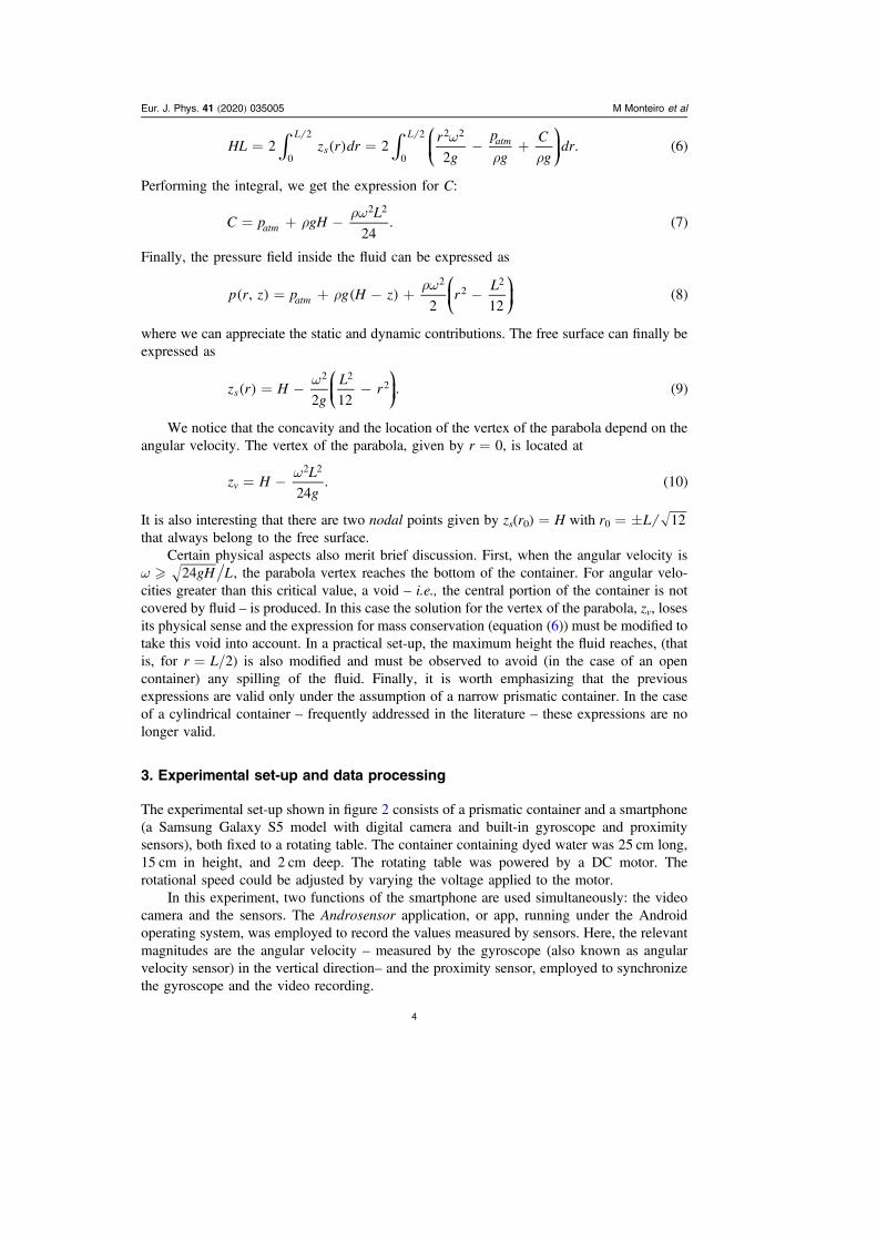
Initially, with the rotating table at rest, we turn on the video camera and start recording sensordata. To synchronize the video and the data provided by the app, we cover simultaneously, for afew seconds, the lens of the camera and the proximity sensor, obtaining in this way a commontime reference for the video and sensor data. The experiment starts by slowly increasing the powersupply – and thus the rotating table angular velocity – while the video camera is recording thesurface of the fluid and the gyroscope sensor is registering the angular velocity. When the angularvelocity reaches the maximum allowed value, the table is gently stopped. Figure 3 shows thetemporal evolution of the angular velocity. The blue arrow indicates the time used to synchronizethe video and the sensor data. After interrupting video and sensor data registration, both files aretransferred to the internet or a personal computer. The Androsensor app stores data as electronicspreadsheets of the .csv (comma separated values) type, in which one column contains the angularvelocity values and another contains the time values. Data can be processed on a computer withthe user’s preferred software. The accompanying video abstract (also available at https://youtu.be/mwP-7tg7b6Q) shows a synopsis of the experimental set-up, video, and data processing.
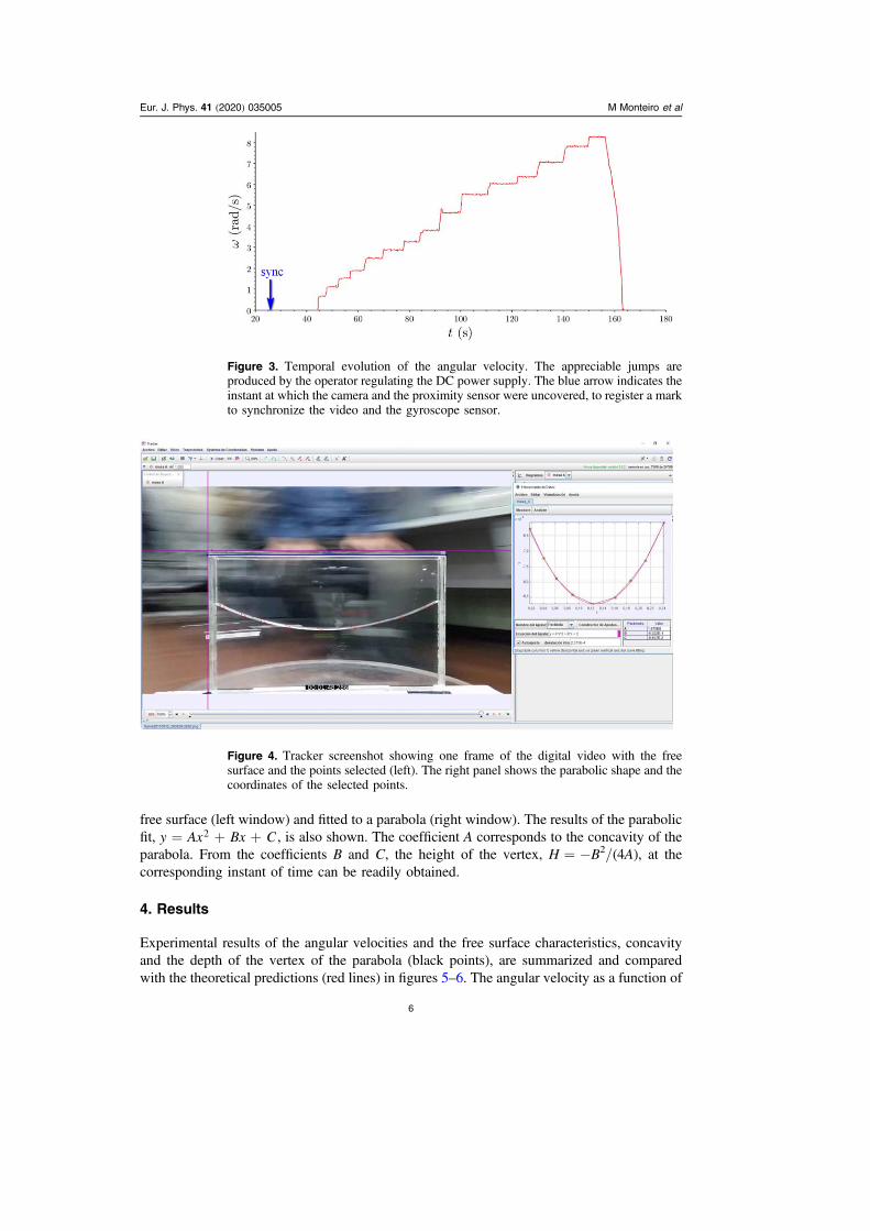
Video recording is analyzed using the Tracker video analysis package [15]. To analyzethe characteristics of the time-evolving surface, we first extract the individual frames from thedigital video. Next, we select 15 frames corresponding to instants of time during theexperiment (and then the different values of the angular velocities shown in figure 3). Theanalysis of each frame, depicted in figure 4, was performed with the aid of Tracker. Severalpoints on the interface – typically eight, labeled in magenta – were manually selected on the
Figure 2. Experimental set-up composed of a narrow container mounted on a rotatingtable. The smartphone, also fixed to the rotating system, supplies both the video of thetime-evolving surface and the angular velocity obtained with the gyroscope.
free surface (left window) and fitted to a parabola (right window). The results of the parabolicfit, = + +y Ax Bx C2 , is also shown. The coefficient A corresponds to the concavity of theparabola. From the coefficients B and C, the height of the vertex, H=−B2/(4A), at thecorresponding instant of time can be readily obtained.
4. Results
Experimental results of the angular velocities and the free surface characteristics, concavityand the depth of the vertex of the parabola (black points), are summarized and comparedwith the theoretical predictions (red lines) in figures 5–6. The angular velocity as a function of
Figure 3. Temporal evolution of the angular velocity. The appreciable jumps areproduced by the operator regulating the DC power supply. The blue arrow indicates theinstant at which the camera and the proximity sensor were uncovered, to register a markto synchronize the video and the gyroscope sensor.
Figure 4. Tracker screenshot showing one frame of the digital video with the freesurface and the points selected (left). The right panel shows the parabolic shape and thecoordinates of the selected points.
Eur. J. Phys. 41 (2020) 035005 M Monteiro et al
6
the concavity of the parabola is plotted in figure 5. In the inset, a least-squares fit is included.The resulting slope of the linear fit is 20.16(4) m·rad2/s2, which, according to equation (9), isin good agreement with 2g.
The height of the parabola vertex as a function of angular velocity squared is plotted infigure 6. The resulting slope of the linear fit is −0.27(1)mm·s2/rad2, which is very similar to thevalue, according to equation (10), given by the model −L2/24g= −0.2655(5)mm·s2/rad2.In addition, the intercept corresponds to the water level with the rotating table at rest. In theexperiment, the value obtained is −7.72(3) cm while the direct value obtained by measuringdirectly on the image is −7.6(2) cm.
Figure 5. Relationship between the angular velocity and the concavity of the fluid surfacefitted to a parabola. The points indicate the experimental results and the solid line the modelprediction. The slope of the linear fit shown in the inset is 20.16(4)m·rad2/s2.
Figure 6. Experimental (black points) and theoretical model (red line) of the height ofthe parabola vertex as a function of the angular velocity. The parameters of the model,slope −0.27(1) mm·s2/rad2 and intercept −7.72(3), were obtained from the linear fitshown in the inset in which the leftmost point corresponding to a small angular velocity(and therefore the most uncertain) was not taken into account.
Eur. J. Phys. 41 (2020) 035005 M Monteiro et al
7
5. Conclusions and prospects
The project aimed to experiment with the free surface of a liquid rotating with a time-dependent angular velocity. Using a smartphone, the shape of the surface and the angularvelocity are simultaneously measured. Using video analysis software, we obtain the coeffi-cients of the parabolic profile which can be related to the angular velocity, the gravitationalacceleration and the water level with the rotating table at rest. The experiment yields verygood agreement with the theoretical model. This simple and inexpensive proposal provides anopportunity for students to engage with challenging aspects of fluid dynamics withoutsophisticated or expensive equipment.
Acknowledgments
We are very grateful to Gustavo Sarasúa, Cecilia Cabeza, and Nicolás Rubido for their kindcooperation. This work was partially supported by the program Física No Lineal, CSICGrupos I+D (Universidad de la República, Uruguay).
ORCID iDs
Martín Monteiro https://orcid.org/0000-0001-9472-2116Arturo C Martí https://orcid.org/0000-0003-2023-8676
References
[1] White F M 2003 Fluid Mechanics (New York, NY: McGraw-Hill)[2] Streeter V L, Wylie E B and Bedford K W 2002 Fluid Mechanics (New York, NY: McGraw-Hill)[3] Fletcher R I 1972 The apparent field of gravity in a rotating fluid system Am. J. Phys. 40 959–65[4] Graf E H 1997 Apparatus for the study of uniform circular motion in a liquid Phys. Teach. 35
427–30[5] Sundström A and Adawi T 2016 Measuring g using a rotating liquid mirror: enhancing laboratory
learning Phys. Educ. 51 053004[6] de Pereira A P and Gomes L E S 2016 Rotating the haven of fixed stars: a simulation of Mach’s
principle Phys. Educ. 51 055016[7] Watzky A 2017 Why Newton’s bucket cannot account for Earth’s rotation Eur. J. Phys. 39 015002[8] Fägerlind C-O and Pendrill A-M 2015 Liquid in accelerated motion Phys. Educ. 50 648[9] Tornaría F, Monteiro M and Marti A C 2014 Understanding coffee spills using a smartphone
Phys. Teach. 52 502–3[10] Monteiro M, Cabeza C, Marti A C, Vogt P and Kuhn J 2014 Angular velocity and centripetal
acceleration relationship Phys. Teach. 52 312–3[11] Monteiro M, Cabeza C and Martí A C 2014 Exploring phase space using smartphone acceleration
and rotation sensors simultaneously Eur. J. Phys. 35 045013[12] Monteiro M, Vogt P, Stari C, Cabeza C and Marti A C 2016 Exploring the atmosphere using
smartphones Phys. Teach. 54 308–9[13] Monteiro M, Stari C, Cabeza C and Martí A C 2017 The polarization of light and Malus’ law using
smartphones Phys. Teach. 55 264–6[14] Monteiro M, Stari C, Cabeza C and Marti A C 2017 Magnetic field ‘flyby’ measurement using a
smartphone’s magnetometer and accelerometer simultaneously Phys. Teach. 55 580–1[15] Brown D 2014 Tracker: free video analysis and modeling tool for physics education https://