Experimental and Numerical Study of Tidal Basin Management around Link Canal:

A Case Study of Bangladesh

Rocky TALCHABHADEL(1), Hajime NAKAGAWA, Kenji KAWAIKE and

Kazuyuki OTA(2)

(1) Department of Civil and Earth Resources Engineering, Kyoto University

(2) Central Research Institute of Electric Power Industry, Japan

Synopsis

The construction of series of polders is the response to the floods. But the obstructions

led to accelerated silt deposition in the rivers. It causes the severe drainage congestion.

Dredging is an enormous task which is costly and again the river faces siltation every time.

De-poldering and then controlled flooding in a particular flooding plain as the tidal basin,

is not a new way of sediment management. Tidal basin acts as sedimentation trap which

allows natural tidal flows up and down in the river system. It is basically shifting the

sedimentation from the riverbed to selected tidal basin. An attempt has been made to assess

the effectiveness of the system through experimental and numerical simulation. It is found

that if the natural river is in equilibrium, the recommended size of the link canal is more

or less equal to the natural width of the river. Furthermore, if the upstream river flow is

reduced, it has resulted in more sedimentation in selected tidal basin.

Keywords: Tidal Basin Management, beel, tidal basin, Suspended Sediment

Concentration, tidal movement, link canal

1. Introduction

For eras, the Bengal delta that constitutes

Bangladesh and India’s West Bengal has been

formed by the sediments carried downstream by

Ganges, Meghna and Brahmaputra river system. In

Bengali, Bangladesh is called nodimatrik desh

(Islam, 2001). This means the rivers gave birth. The

Bengal delta has been home to a dynamic interplay

of water and land (Staveren et al., 2017). The South

West (SW) region of Bangladesh is a tidal basin

active tidal channels and large parts are still going

through active deltaic formations (Haque et al.,

2015). It is characterized by unique brackish water

ecosystem interspersed with sensitive tide-

dominated rivers, streams and water-filled

depressions. A considerable area in the SW region is

below the high water level of spring tide.

2. Literature review

2.1 Sediment management from impoldering to

de-poldering

Before construction of the polders, river tides

would inundate vast tracts of lowland twice a day

due to astronomical tide from the Bay of Bengal

(Rahman and Salehin, 2013; Tutu, 2005). Much of

these lowlands are beels, a Bengali term used for

relatively large depressions that accumulate water

(Banglapedia, 2012). The Coastal Embankment

Project (CEP) was a response to the large flood in

1954. Construction and development of

embankments started in 1961. The polders were

constructed into encircled earthen embankments

around depressions keeping the main tidal channel

outside the polder. The embankments were not

constructed to protect against water levels during

京都大学防災研究所年報 第 60 号 B 平成 29 年

DPRI Annuals, No. 60 B, 2017

― 719 ―

cyclones.

The initial outcomes of the polders were quite

rewarding both economically and socially. The

polder embankments not only prevented floods from

overflowing the land but also halted the deposition

of silt and clay on the former floodplains. The

obstructions by polder system led to accelerated silt

deposition and sediment accumulation in region’s

rivers and channels. The resulting dearth of land

formation left floodplains inside the polders lower

than riverbanks outside the polders (Rezaie and

Naveram, 2013). Vast tracts of land went under

water semi-permanently, i.e. for 6 months or more in

a year, as the water could not be drained away

overland, nor could it be discharged.

To solve this issue, a certain area is kept aside as

tidal floodplain by doing temporary de-poldering.

The link canal so created connects the tidal basin

(selected beel) with the river (Ibne Amir et al., 2013).

Muddy water enters the tidal basin during high tide

with a thick concentration of sediments, depositing a

major portion of suspended sediments before

flowing back towards the sea during low tide (Ibne

Amir et al., 2013; Khadim et al., 2013; Kibria, 2011).

Institutionally it was termed Tidal River

Management (TRM).

2.2 Concept of TRM/TBM

TRM is the scientific term given to the age-old

practice of flood and water management where a

temporary de-poldering is done by connecting the

tidal rivers with designated low land. The concept is

simple. The natural high tide of river enters the low

lying beel, leaves a part of sediment to be deposited

and goes back to the ocean. Since this process does

not allow sediments to be deposited on the river bed,

the depth of river bed also increases and makes the

river congestion free (Shampa and Pramanik, 2012).

In addition, if the riverbed decline advances, the

influence would be exerted to the upper stream. Akai

et al. (1990) termed it “The UTSURO”. The process

is continued for several years (usually 3 to 4 years,

the duration depends on the size of the tidal basin).

Such tidal basins are to be rotated among various

lowlands within the system so that farmers of one

tidal basin do not have to suffer for a long time, the

process known as Tidal Basin Management (TBM).

TBM involves the natural tide movement in rivers

and taking full advantage of it (Ibne Amir et al.,

2013; Shampa and Pramanik, 2012; Talchabhadel et

al., 2016a). Fig. 1 shows the conceptual model of

TBM. This sedimentation would occur into the

riverbed if it is not utilized for storage as

sedimentation trap (Ibne Amir et al., 2013; Paul et

al., 2013; Rahman and Salehin, 2013).

When one TBM beel has achieved the required

raising of the land, then another TBM beel will take

the sediment load that comes in with the tide. There

should not be any time gap in between closing and

operation of successive beels (Ullah and Mahmud,

2017). If the rotation is not carried out systematically,

then the tides are very likely to drop their sediments

in the river channel themselves (Nowreen et al.,

2014). Since the TBM process is the participatory

approach where the people of identified beel have to

sacrifice their land for an intended period (3-5 years),

a proper compensation to the affected people should

be ensured.

Fig. 1 Conceptual model of TRM/TBM (Source :

Author ) and location of proposed tidal basin in

KJDRP (Source: Rahman and Salehin, 2013)

― 720 ―

2.3 Tidal prism – Inlet area relationships

Jarrett (1976) has investigated to develop the tidal

prism and inlet area relationship originally

developed by O’Brien in 1931 as an empirical

relationship based on 10 tidal inlets. The study

focused on the determination of the effect of inlet

configuration for a number of realistic inlet shapes

and tidal conditions. The first known published

relationship between the cross-sectional area of the

tidal inlet and the tidal prism were given by LeConte

in 1905 for harbor entrances on the Pacific coast.

The obvious fact that large inlets are found at large

bays whereas small inlets at small bays suggested

O’Brien (1969) suggested a relationship between

equilibrium flow area and tidal prism.

𝐴 = 𝑎 ∗ 𝑃𝑛 (1)

where A is the minimum flow cross section of the

entrance, P is the tidal prism corresponding to the

diurnal or spring range of tide and a & n are

coefficients vary from entrance to entrance. Stive

and Rakhorst (2008) has reviewed some of the

popular Dutch and US empirical relationships

between inlet cross-section and tidal prism with

theoretical elaborations both qualitatively and

quantitatively. Many researchers (Hume and

Herdendorf, 1993; O’Brien, 1969; Powell et al.,

2006; Rakhorst, 2007; Van de Kreeke and Haring,

1980) have suggested to applying the Equation 1

with best-fitting values of a and n. The approach of

Kraus (1998) is somewhat different. He introduced

the representative shear stress needs to attain a value

of the magnitude of the critical shear stress for

sediment motion.

𝜏∗𝑐 (𝜎

𝜌− 1)𝑔𝑑 = 𝑔

𝑢2

𝐶2= 𝑔 (

2𝑃

𝐶𝐴𝑇)2

(2)

where 𝜏∗𝑐 is critical shear stress according to

Shields, is the density of sediment particles, is

the water density, d is the diameter of sediment

particles, u is the characteristic flow velocity

(realizing discharge Q = A*u, Qmax = 2P/T where T

is the tidal period) and C is dimensionless Chezy

coefficient.

Fig. 2 Equilibrium relationship between tidal prism

and river cross-sectional area (Source : Rahman et

al., 2015; Shampa and Pramanik, 2012)

Some rearrangement of Equation 1.1 gives

𝐴 = (4

𝜏∗𝑐(𝜎

𝜌−1)𝑔𝑑𝐶2𝑇2

)

1/2

𝑃 (3)

The equation (3) could be compared with equation

1.1 where a = (4

𝜏∗𝑐(𝜎

𝜌−1)𝑔𝑑𝐶2𝑇2

)

1/2

and n = 1. Stive

and Rakhorst (2008) has calculated the value of a to

be 0.9*10-4 for sediment size 300 𝜇 m. Some

researchers have attempted to express the Chezy

coefficient in terms of Manning coefficient ( 𝐶 =

ℎ1/6

𝑛) where h is characteristics water depth and n is

the Manning coefficient.

From above, it is clear that the entrance cross-

section A and the tidal prism P could be expressed

with a relation. For determining the consistent

relationship abundant amount of field-based data of

the tidal river is needed because the coefficients vary

from entrance to entrance. The sample of one of the

equilibrium relationship for a coastal river of

Bangladesh is shown in Fig. 2.

2.4 Study of TRM/TBM

Many studies have done different types of

qualitative analysis of TRM/TBM and its relation

with disaster, ecosystem, environment, agriculture,

flood, and sediment management. Very limited

researchers have attempted to numerically simulate

the process of TBM in Bangladesh and almost nil via

experimental analysis.

― 721 ―

Shampa and Pramanik (2012) has simulated

numerically for the Kobadak River to assess the

effectiveness of proposed TBM in the beel Jalalpur.

The research proposed that TBM operation is more

effective with the construction of the cross dam

during the dry period. It is also mentioned that the

monsoon flow does not erode the deposited sediment

on river bed because of high sediment concentration

during monsoon.

Ibne Amir et al., (2013) has numerically

simulated in two beels: One is East beel Khuksia

where TBM has fully implemented, and another is

beel Kapalia where TBM is supposed to operate. The

technical feasibilities using economic analysis were

analyzed using the numerical modeling. The option

that includes, constructing embankments along both

banks of the main channels through the tidal basin

and thereby allowing sedimentation by gradually

cutting the embankment part by part from upstream

to downstream, has been suggested in their research.

Furthermore, dividing the beel into compartment had

better results than allowing TBM in the whole basin

at the same time. In the research, it is also suggested

that the beels with greater tidal influence are more

suitable for TBM operation.

Rahman et al. (2015) has developed a numerical

model for two potential beels: Sukdebpur beel along

the left bank of Betna River and another Ticket beel

along the right bank of Marirchap River. The

research showed that in addition to the

dredging/excavation, implementation of TBM to

trap up the incoming sediment inside the basin was

needed for sustainable sediment and drainage

management.

Ogawa and Sawai (2013) has done similar

research for the Yellow River for river bed

sedimentation control using a tidal reservoir by

numerical analysis. In this study, the primary focus

is the control of riverbed sedimentation rather than

the land heightening or deposition of sediment. Akai

et al. (1990) called the process of advancement of

riverbed decline as “The UTSURO”. The research

concluded that the tidal reservoir is effective in a

riverbed decline. However, the longer the distance

between the connecting point and estuary, the

smaller the degree of the river bed decline in the

downstream.

3. Objectives of the study

The literature review reveals that a number of

comprehensive studies on TRM/TBM are available.

These studies cover a wide range of analysis

regarding appropriate planning, design, and

implementation of TBM in a coastal river.

Furthermore, such an innovative scientific approach

which is again semi-natural process has been related

to institutional management, socio-economical

barriers by many researchers. The implications of

TBM as disaster management approach, ecosystem

and environmentally friendly approach and

ultimately sustainable sediment management

approach have been discussed by them.

Some of the researchers have discussed regarding

the mainstreaming of TBM for participatory

environmental governance, flood policy, climate

change adaptation, disaster management, drainage

rehabilitation project and many others. Few

researchers also carried out numerical simulation for

effective planning, the design of potential beels and

also for monitoring and evaluation of operated beels.

It clearly shows the TBM process has been one of

the integral parts of sediment management for tidal

rivers in Bangladesh. But the experimental analysis

of such complicated process is very rare.

In this research, the attempts have been made to

assess the effectiveness of TRM/TBM through

small-scale laboratory experiments. One significant

hydraulic fact is that the faster the flow is, the more

sediment it can carry with it. One of the key

governing factors of the flow is the opening size of

link canal. For the establishment of a consistent

relationship between tidal prism and minimum

cross-sectional area, an abundant amount of real

field data of the tidal rivers are needed.

To inspect the effectiveness of TBM exploring

different opening sizes and to compare with

available empirical relations, this research has

attempted to carry out small-scale laboratory

experiments. Two-dimensional (2D) numerical

simulation models have been developed to compare

with experimental results and to analyze different

alternatives to suggest the sustainable sediment

management. The experimental and numerical

analysis are implemented to analyze the physical

mechanism of the sediment transport and deposition

― 722 ―

during the operation of TBM process. The complex

phenomena and local mechanism during the

experiment around a sharp bend or any structure

have attempted to discuss with the real scenario and

attempted to analyze by three-dimensional (3D)

numerical simulation.

4. Experiments and Numerical

Simulations

4.1 Experimental analysis

The experiments were carried out in a flume

located at the Ujigawa open laboratory of Disaster

Prevention Research Institute, Kyoto University.

The schematic view is illustrated in Fig. 3. See

(Talchabhadel et al., 2017a, 2017b) for a detailed

explanation of the experimental methodologies.

TBM capitalizes on the natural movement of tidal

water. To represent alternative high and low tidal

flow, an adjustable gate was used. To represent high

tide, the gate was closed for 2 mins and downstream

flow from water pump was supplied along with dry

sediment supply from sediment feeder. After then,

the gate was opened for next 2 min. At that time

downstream supply of water and sediment were

stopped representing low tide. Same processes were

repeated. Two complete tidal cycles in a day in the

real case of Bangladesh (Kibria, 2011) here is

attempted to represent with 8 min experimental case

(i.e. 2 min high tide and 2 min low tide for one tidal

cycle). Four cases with different opening sizes were

investigated varying the size of the opening canal

towards tidal basin.

4.2 Numerical Simulations

Fig. 4 Boundary condition treatment in

numerical simulation

The experimental boundary condition of an

adjustable condition has been applied in the

numerical simulation (shown in Fig. 4). The

boundary at outlet shown in black in Fig. 4 switches

to the side wall and the outlet along with the time.

When the boundary at outlet switches to the side wall,

the input high tidal discharge and sediment supply

are also provided.

4.2.1 2D simulation

The simulation model used in this study is

structural gridded two-dimensional (2D) unsteady

flow model based on a shallow-water equation.

Finite Difference Method (FDM) is applied. To

solve the equations, leap frog difference scheme is

employed.

Fig. 3 Schematic view of experimental setup

― 723 ―

Continuity equation

𝜕ℎ

𝜕𝑡+

𝜕𝑀

𝜕𝑥+

𝜕𝑁

𝜕𝑦= 0 (4)

Momentum equation

𝜕𝑀

𝜕𝑡+

𝜕(𝑢𝑀)

𝜕𝑥+

𝜕(𝑢𝑀)

𝜕𝑦= −𝑔ℎ

𝜕𝐻

𝜕𝑥−

𝑔𝑛2𝑢√𝑢2+𝑣2

ℎ1/3 (5)

𝜕𝑁

𝜕𝑡+

𝜕(𝑢𝑁)

𝜕𝑥+

𝜕(𝑣𝑁)

𝜕𝑦= −𝑔ℎ

𝜕𝐻

𝜕𝑦−

𝑔𝑛2𝑣√𝑢2+𝑣2

ℎ1/3 (6)

where, h is the water depth, M (=uh) and N (=vh)

are fluxes in the x and y directions, u and v are

velocities in the x and y directions, H is the water

level, g is the acceleration of gravity, and n is the

Manning’s roughness coefficient. Sediment

transport is simulated using the following equations:

Suspended sediment transport calculation

Suspended sediment transport is simulated using the

following equations.

𝜕(𝐶ℎ)

𝜕𝑡+

𝜕(𝐶𝑀)

𝜕𝑥+

𝜕(𝐶𝑁)

𝜕𝑦= 𝐷 (

𝜕2(𝐶ℎ)

𝜕𝑥2+

𝜕2(𝐶ℎ)

𝜕𝑦2) + 𝐸 +

𝐶𝑤 (7)

where C is the concentration of sediment, D is a

coefficient of diffusion, E is the parameter of

flowing up and w is the settling velocity. Given the

situation, D was set to 0.1 m2/s (Hashimoto et al.,

2016).

In this study, the settling velocity is calculated

with the Rubey’s formula (Rubey, 1933).

𝑤 = √2

3(𝜎

𝜌− 1)𝑔𝑑 +

36𝜈2

𝑑2−

6𝜈

𝑑 (8)

where is the density of sediment particles, is

the water density, d is the diameter of sediment

particles and 𝜈 is the coefficient of kinematic

viscosity of water.

The upward flux is assumed to be under

equilibrium condition. The equilibrium

concentration is calculated using the van Rijn

empirical formula (Van Rijn, 1984a).

𝐸 = 𝑤𝐶∗ (9)

𝐶∗ = 0.015𝑑𝑇1.5

𝑎𝐷∗0.3 (10)

where 𝑎 is the reference is level taken 0.05h, 𝐷∗

is the particle size parameter and T is a

dimensionless excess bed shear stress parameter. 𝐷∗

and T are defined by the equation 3.8 and 3.9.

𝐷∗ = 𝑑 [(𝜎

𝜌−1)𝑔

𝜈2]

1/3

(11)

𝑇 =𝜏∗−𝜏∗𝑐

𝜏∗𝑐 (12)

where 𝜏∗ and 𝜏∗𝑐 are the dimensionless shear

stress and critical shear stress according to the

Shields. The grain related shear stress parameter 𝜏∗

is calculated by considering Chezy’s equation.

𝜏∗ = 𝑢∗2

(𝜎

𝜌−1)𝑔𝑑

(13)

𝑢∗ = √𝑔𝑢

𝐶′ (14)

where 𝐶′ = grain related Chezy’s roughness

coefficient which for rough flow is given by :

𝐶′ = 18 𝑙𝑜𝑔 (12ℎ

𝑘𝑠) (15)

where ks = grain roughness. For smooth bed, ks =

0, and for a stationary flat bed in laboratory

experiments, ks is usually set to the median diameter

d50 of bed material because there is only sand-grain

roughness on the bed. For stationary flat bed in real

rivers, ks should theoretically also be about d50, but

in practice usually somewhat higher values are

adopted, e.g. Van Rijn (1984b) relate the grain

roughness to the coarse 90 th percentile (d90) of grain

size distribution, i.e. ks=3d90. By contrast Engelund

and Fredsøe (1976), Nielsen (1992) and Soulsby and

Damgaard (2005) related the grain roughness to the

median grain size (d50) i.e. ks=2.5d50 which is used

in the present study. The dimensionless critical shear

stress 𝜏∗𝑐 for the sediment size d is evaluated with

the Iwagaki formula (Iwagaki, 1956).

𝜏∗𝑐 =

{

0.05 𝑖𝑓 𝑅∗ ≥ 671.0

0.00849𝑅∗3/11 𝑖𝑓 162.7 ≤ 𝑅∗ < 671.0

0.034 𝑖𝑓 54.2 ≤ 𝑅∗ < 162.7

0.195𝑅∗−7/16 𝑖𝑓 2.14 ≤ 𝑅∗ < 54.2

0.14 𝑖𝑓 𝑅∗ < 2.14

(16)

― 724 ―

where

𝑅∗ = √(

𝜎

𝜌−1)𝑔𝑑3

𝜈 (17)

Bedload transport calculation

The bed load transport rate is calculated by the

equation of (Ashida and Michiue, 1972).

𝑞𝑏

√(𝜎

𝜌−1)𝑔𝑑3

= 17𝜏∗𝑒

3

2 (1 −𝑢∗𝑐

𝑢∗) (1 −

𝜏∗𝑐

𝜏∗) (18)

where 𝑞𝑏 is the bed load discharge (m2/s),𝜏∗, 𝜏∗𝑐

and 𝜏∗𝑒 are dimensionless shear stress, critical

shear stress (Iwagaki, 1956) and effective shear

stress, respectively; 𝑢∗ and 𝑢∗𝑐 are friction

velocity and critical friction velocity (m/s),

respectively. These parameters are calculated

through following relations:

𝜏∗𝑐 = 𝑢∗𝑐

2

(𝜎

𝜌−1)𝑔𝑑

(19)

𝜏∗𝑒 = 𝑢∗𝑒

2

(𝜎

𝜌−1)𝑔𝑑

(20)

where 𝑢∗𝑒 is effective friction velocity. The

effective shear stress 𝜏∗𝑒 is calculated by taking the

account of equivalent roughness height ks

quantifying the influence of roughness elements

such as sand grains, sand waves (including ripples,

dunes and antidunes) and other bed form. For sand

wave bed, ks should be related to the height of the

sand waves, (Van Rijn, 1984b) proposed the

following relationship, which is used in the present

study to replicate the bed form of experimental result.

𝑘𝑠 = 2.5𝑑50 + 1.1∆(1 − 𝑒−25𝜓)(25 − 𝑇) (21)

where T is an excess bed shear stress parameter

defined earlier and 𝜓 =Δ

Λ, is the bed-form steepness,

Δ and Λ the height and length of the bed forms.

The bed-form steepness is calculated from

𝜓 =Δ

Λ= 0.015 (

𝑑50

ℎ) (1 − 𝑒−0.5𝑇)(25 − 𝑇) (22)

Bedload deformation

The bed level changes are computed from the

information of bed load and suspended load

transport rates using the mass-balance equation.

(1 − 𝜆)𝜕𝑧𝑏

𝜕𝑡+

𝜕𝑞𝑏𝑥

𝜕𝑥+

𝜕𝑞𝑏𝑦

𝜕𝑦+ (𝐸 − 𝐶𝑤) = 0 (23)

where 𝜆 is the sediment porosity, 𝑞𝑏𝑥 and 𝑞𝑏𝑦

are bed load transport rates in the x and y directions.

4.2.2 3D simulation

The simulation model used in this study is

OpenFOAM (Open Field Operation and

Manipulation which is primarily a C++ toolbox for

the customization and extension of numerical

solvers for continuum mechanics problems,

including computational fluid dynamics (CFD). It

comes with a growing collection of pre-written

solvers applicable to a wide range of problems. It is

released open source under the GPL (OpenCFD Ltd.,

2009a, 2009b).

The hydrodynamic model consists of a RANS

(Reynolds-averaged Navier-Stokes) model, k-ω SST

(shear stress transport) turbulence closure, and a

volume of fluid (VOF) method for capturing the

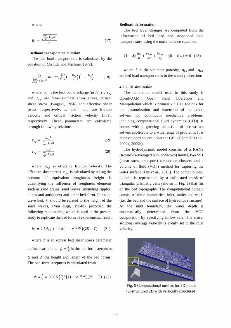
water surface (Ota et al., 2016). The computational

domain is represented by a collocated mesh of

triangular prismatic cells (shown in Fig. 5) that fits

on the bed topography. The computational domain

consist of three boundaries: inlet, outlet and walls

(i.e. the bed and the surface of hydraulics structure).

At the inlet boundary, the water depth is

automatically determined from the VOF

computation by specifying inflow rate. The cross-

sectional average velocity is evenly set to the inlet

velocity.

Fig. 5 Computational meshes for 3D model

(unstructured 2D with vertically structured)

― 725 ―

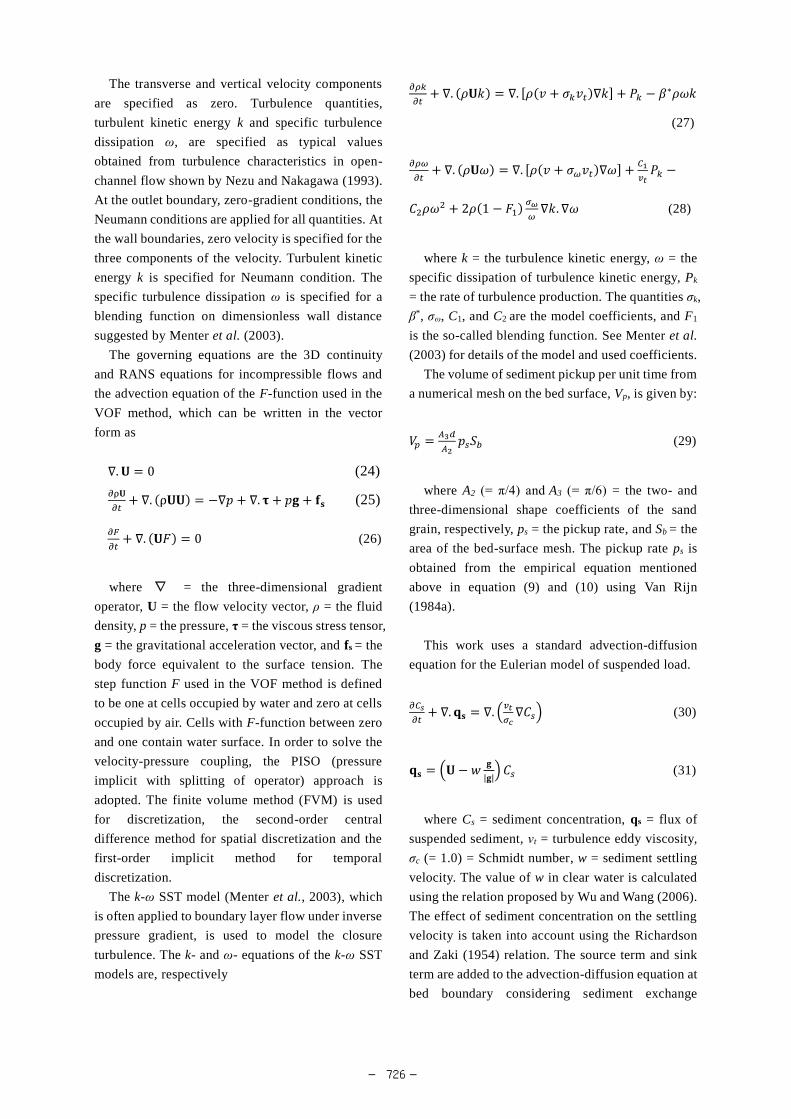
The transverse and vertical velocity components

are specified as zero. Turbulence quantities,

turbulent kinetic energy k and specific turbulence

dissipation ω, are specified as typical values

obtained from turbulence characteristics in open-

channel flow shown by Nezu and Nakagawa (1993).

At the outlet boundary, zero-gradient conditions, the

Neumann conditions are applied for all quantities. At

the wall boundaries, zero velocity is specified for the

three components of the velocity. Turbulent kinetic

energy k is specified for Neumann condition. The

specific turbulence dissipation ω is specified for a

blending function on dimensionless wall distance

suggested by Menter et al. (2003).

The governing equations are the 3D continuity

and RANS equations for incompressible flows and

the advection equation of the F-function used in the

VOF method, which can be written in the vector

form as

∇. 𝐔 = 0 (24)

∂ρ𝐔

𝜕𝑡+ ∇. (ρ𝐔𝐔) = −∇𝑝 + ∇. 𝛕 + 𝑝𝐠 + 𝐟𝐬 (25)

∂𝐹

𝜕𝑡+ ∇. (𝐔𝐹) = 0 (26)

where ∇ = the three-dimensional gradient

operator, U = the flow velocity vector, ρ = the fluid

density, p = the pressure, τ = the viscous stress tensor,

g = the gravitational acceleration vector, and fs = the

body force equivalent to the surface tension. The

step function F used in the VOF method is defined

to be one at cells occupied by water and zero at cells

occupied by air. Cells with F-function between zero

and one contain water surface. In order to solve the

velocity-pressure coupling, the PISO (pressure

implicit with splitting of operator) approach is

adopted. The finite volume method (FVM) is used

for discretization, the second-order central

difference method for spatial discretization and the

first-order implicit method for temporal

discretization.

The k-ω SST model (Menter et al., 2003), which

is often applied to boundary layer flow under inverse

pressure gradient, is used to model the closure

turbulence. The k- and ω- equations of the k-ω SST

models are, respectively

∂𝜌𝑘

𝜕𝑡+ ∇. (𝜌𝐔𝑘) = ∇. [𝜌(𝑣 + 𝜎𝑘𝑣𝑡)∇𝑘] + 𝑃𝑘 − 𝛽

∗𝜌𝜔𝑘

(27)

∂𝜌𝜔

𝜕𝑡+ ∇. (𝜌𝐔𝜔) = ∇. [𝜌(𝑣 + 𝜎𝜔𝑣𝑡)∇𝜔] +

𝐶1

𝑣𝑡𝑃𝑘 −

𝐶2𝜌𝜔2 + 2𝜌(1 − 𝐹1)

𝜎𝜔

𝜔∇𝑘. ∇𝜔 (28)

where k = the turbulence kinetic energy, ω = the

specific dissipation of turbulence kinetic energy, Pk

= the rate of turbulence production. The quantities σk,

β*, σω, C1, and C2 are the model coefficients, and F1

is the so-called blending function. See Menter et al.

(2003) for details of the model and used coefficients.

The volume of sediment pickup per unit time from

a numerical mesh on the bed surface, Vp, is given by:

𝑉𝑝 =𝐴3𝑑

𝐴2𝑝𝑠𝑆𝑏 (29)

where A2 (= π/4) and A3 (= π/6) = the two- and

three-dimensional shape coefficients of the sand

grain, respectively, ps = the pickup rate, and Sb = the

area of the bed-surface mesh. The pickup rate ps is

obtained from the empirical equation mentioned

above in equation (9) and (10) using Van Rijn

(1984a).

This work uses a standard advection-diffusion

equation for the Eulerian model of suspended load.

𝜕𝐶𝑠

𝜕𝑡+ ∇. 𝐪𝐬 = ∇. (

𝑣𝑡

𝜎𝑐∇𝐶𝑠) (30)

𝐪𝐬 = (𝐔 − 𝑤𝐠

|𝐠|) 𝐶𝑠 (31)

where Cs = sediment concentration, qs = flux of

suspended sediment, νt = turbulence eddy viscosity,

σc (= 1.0) = Schmidt number, w = sediment settling

velocity. The value of w in clear water is calculated

using the relation proposed by Wu and Wang (2006).

The effect of sediment concentration on the settling

velocity is taken into account using the Richardson

and Zaki (1954) relation. The source term and sink

term are added to the advection-diffusion equation at

bed boundary considering sediment exchange

― 726 ―

between bed load and suspended load as:

𝐪𝐬. 𝐧 =∑ 𝑉𝑡

(𝑛)−𝑉𝑠𝑒𝑡𝑡𝑙𝑒𝑛

𝑆𝑏 (32)

𝑉𝑠𝑒𝑡𝑡𝑙𝑒 = 𝑤𝑠𝐶𝑠𝑆𝑏 (33)

where the summation of Vt(n) represents the total

volume of sediments which is transited into

suspension at each time step after pick-up. The

existing formula of suspended sediment

concentration usually assumes equilibrium state of

sediment concentration near the bed and defines the

reference height such as 5 % of the water depth used

by Van Rijn (1984a). The advection-diffusion of

suspended load is therefore solved in whole

computational cells in which water occupies:

Using the volumes of sediment pickup and

sediment deposition, which are calculated as

previously described, the temporal variation in bed

elevation is expressed as follows:

𝜕𝑧𝑏

𝜕𝑡=

𝐴1𝐴2

𝐴3

∑ 𝑉𝑑(𝑛)

𝑛 −𝑉𝑝

𝑆𝑏,𝑝 (34)

where zb = the bed elevation, A1 (= 1.0) = the

shape coefficient of the sediment particles, and Sb,p

= mesh area of the bed surface cell projected onto a

horizontal plane where sediment is deposited. The

summation of Vd(n) represents the total volume of

deposited sediments at each time step after pick-up.

5. Results and discussions

The experimental results, verification of the

developed numerical models and numerical analysis

results are discussed in this section.

5.1 Experimental results and discussions

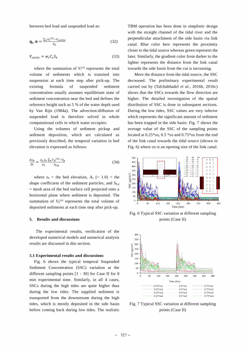
Fig. 6 shows the typical temporal Suspended

Sediment Concentration (SSC) variation at the

different sampling points [1 - 30] for Case II for 8

min experimental time. Similarly, in all 4 cases,

SSCs during the high tides are quite higher than

during the low tides. The supplied sediment is

transported from the downstream during the high

tides, which is mostly deposited in the side basin

before coming back during low tides. The realistic

TBM operation has been done in simplistic design

with the straight channel of the tidal river and the

perpendicular attachment of the side basin via link

canal. Blue color here represents the proximity

closer to the tidal source whereas green represent the

later. Similarly, the gradient color from darker to the

lighter represents the distance from the link canal

towards the side basin from the cut is increasing.

More the distance from the tidal source, the SSC

decreased. The preliminary experimental result

carried out by (Talchabhadel et al., 2016b, 2016c)

shows that the SSCs towards the flow direction are

higher. The detailed investigation of the spatial

distribution of SSC is done in subsequent sections.

During the low tides, SSC values are very inferior

which represents the significant amount of sediment

has been trapped in the side basin. Fig. 7 shows the

average value of the SSC of the sampling points

located at 0.25*os, 0.5 *os and 0.75*os from the end

of the link canal towards the tidal source (shown in

Fig. 6) where os is an opening size of the link canal.

Fig. 6 Typical SSC variation at different sampling

points (Case II)

Fig. 7 Typical SSC variation at different sampling

points (Case II)

0

50

100

150

200

250

300

350

400

0 60 120 180 240 300 360 420 480

SS

C (

gm

/m3)

Time (Sec)

0.25*os1 0.5*os1 0.75*os1

0.25*os2 0.5*os2 0.75*os2

0.25*os3 0.5*os3 0.75*os3

0.25*os4 0.5*os4 0.75*os4

― 727 ―

During the high tide, in case I and case II the

average values of the SSC at 0.75*os are found to be

almost negligible compared to the average values of

the SSC at 0.25*os i.e. 13.5 % for case I and 15.6%

for case II. Again, the average values of the SSC at

0.5*os are found to be around one-third of the SSC

at 0.25*os i.e. 29.4 % for case I and 36.1% for case

II. It clearly indicated that the larger size of opening

has not been utilized for the transport of the sediment.

In the case of narrower opening, the opening sizes

have been utilized effectively. The average values of

the SSC at 0.75*os are found to be around half of the

SSC at 0.25*os i.e. 46.37 % for case III and 57.7 %

for case IV. Again, the average values of the SSC at

0.5*os are found to be significant with more than

half of the SSC at 0.25*os i.e. 57.3 % for case III and

78.9 % for case IV.

During the low tide, the SSC measured at

sampling points around the link canal shows greater

values in the narrower opening cases (i.e. case III

and case IV) than the wider opening cases (case I and

case II). It indicates that during the low tide, the

water coming back from the side basin has greater

shear stress in narrower opening cases than wider

opening cases which promotes in the erosion of

deposited sediment around the link canal which

effectively demonstrates the phenomena of TBM.

Fig. 8 shows the typical spatial distribution of SSC

for Case IV for 4 min experimental time. The line

graph at the top shows the temporal variation of the

SSC at the black dotted location shown in Fig. 8.

Fig. 8 Typical SSC spatio-temporal variation (Case

IV)

Compared to the SSCs at high tide, the SSCs at

low tide are almost constant throughout and the

magnitude of SSCs are also very lesser compared to

SSCs at high tide. In space, the lateral distribution of

SSC is more or less symmetrical progressing form

the opening of the link canal. It also shows similar

results of the greater the distance from the tidal

source, lesser is the SSC. But due to the limited size

of the side basin, the wall effects are clearly seen.

The SSCs at the sampling points near to the side

walls are higher than the nearby sampling points.

The bed level measurements from the laser

displacement sensor were done around the link canal.

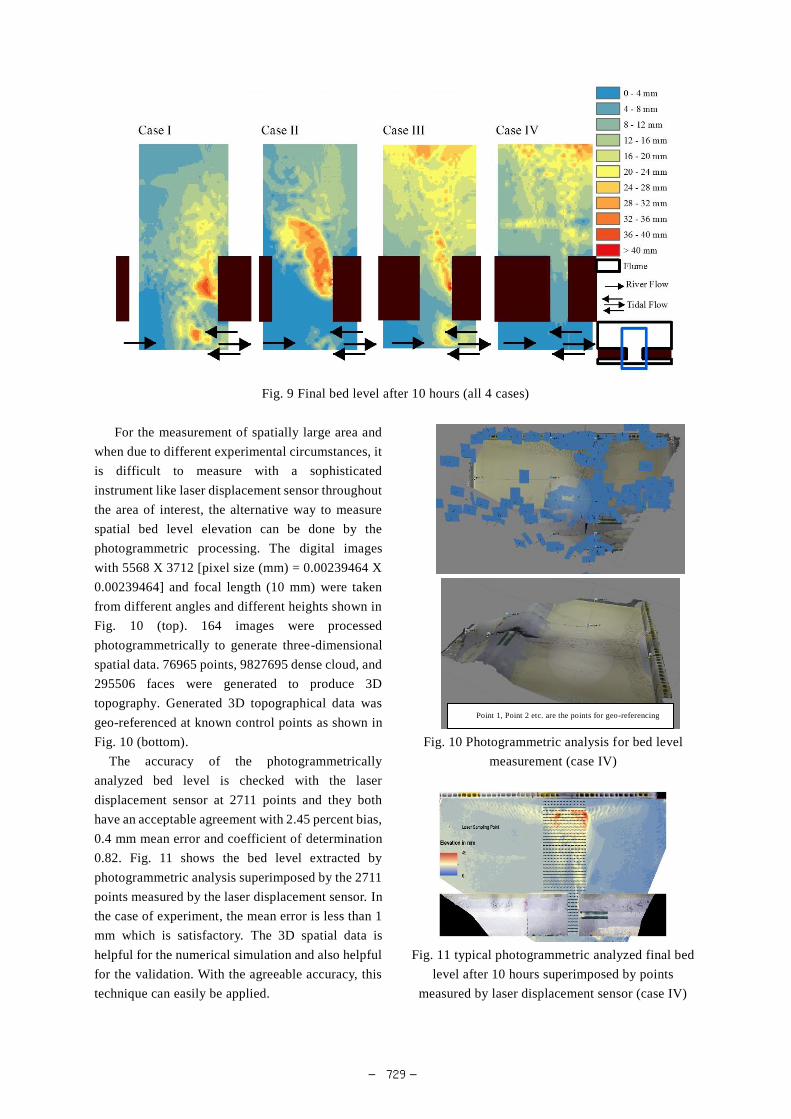
Fig. 9 shows the final bed level condition after 10

hours of the experiment for all 4 cases. In case I, it

is quite clear that the spacious width has not been

properly consumed for the sediment transport and

deposition. In case II, the sediment has been

transported and deposited in a substantial amount but

on the link canal itself, a huge amount of sediment

gets deposited. The flow during the low tide, when it

flows out from the side basin, has not sufficient shear

stress to erode the deposited sediment around the

link canal. In case III, a significant amount of the

sediment has been transported and deposited in the

side basin along with significant erosion during the

low tide. Similarly, in case IV, the shear stress

developed during the low tide is sufficient to erode

the sediment from the link canal.

The latter two cases (i.e. case III and case IV) that

are nearly equaled to the width of the river

effectively demonstrates the realistic operation of

TBM which is needed to solve the drainage

congestion. To suggest the optimum size of the

opening size, more experiments supported by

numerical simulations are needed with varying

opening sizes. Further analysis has been done

subsequent section using the numerical simulation to

represent the experimental condition. The current

experimental research has demonstrated effective

TBM process in the narrower opening cases (case III

and case IV) rather than wider opening sizes (case I

and case II). Moreover, it can also be inferred that if

the existing river is not constrained by any civil

structure and human interventions (i.e. it is in tidal

equilibrium), then the recommended opening size of

the link canal is almost equaled to the natural width

of the river.

― 728 ―

Fig. 9 Final bed level after 10 hours (all 4 cases)

For the measurement of spatially large area and

when due to different experimental circumstances, it

is difficult to measure with a sophisticated

instrument like laser displacement sensor throughout

the area of interest, the alternative way to measure

spatial bed level elevation can be done by the

photogrammetric processing. The digital images

with 5568 X 3712 [pixel size (mm) = 0.00239464 X

0.00239464] and focal length (10 mm) were taken

from different angles and different heights shown in

Fig. 10 (top). 164 images were processed

photogrammetrically to generate three-dimensional

spatial data. 76965 points, 9827695 dense cloud, and

295506 faces were generated to produce 3D

topography. Generated 3D topographical data was

geo-referenced at known control points as shown in

Fig. 10 (bottom).

The accuracy of the photogrammetrically

analyzed bed level is checked with the laser

displacement sensor at 2711 points and they both

have an acceptable agreement with 2.45 percent bias,

0.4 mm mean error and coefficient of determination

0.82. Fig. 11 shows the bed level extracted by

photogrammetric analysis superimposed by the 2711

points measured by the laser displacement sensor. In

the case of experiment, the mean error is less than 1

mm which is satisfactory. The 3D spatial data is

helpful for the numerical simulation and also helpful

for the validation. With the agreeable accuracy, this

technique can easily be applied.

Fig. 10 Photogrammetric analysis for bed level

measurement (case IV)

Fig. 11 typical photogrammetric analyzed final bed

level after 10 hours superimposed by points

measured by laser displacement sensor (case IV)

Point 1, Point 2 etc. are the points for geo-referencing

― 729 ―

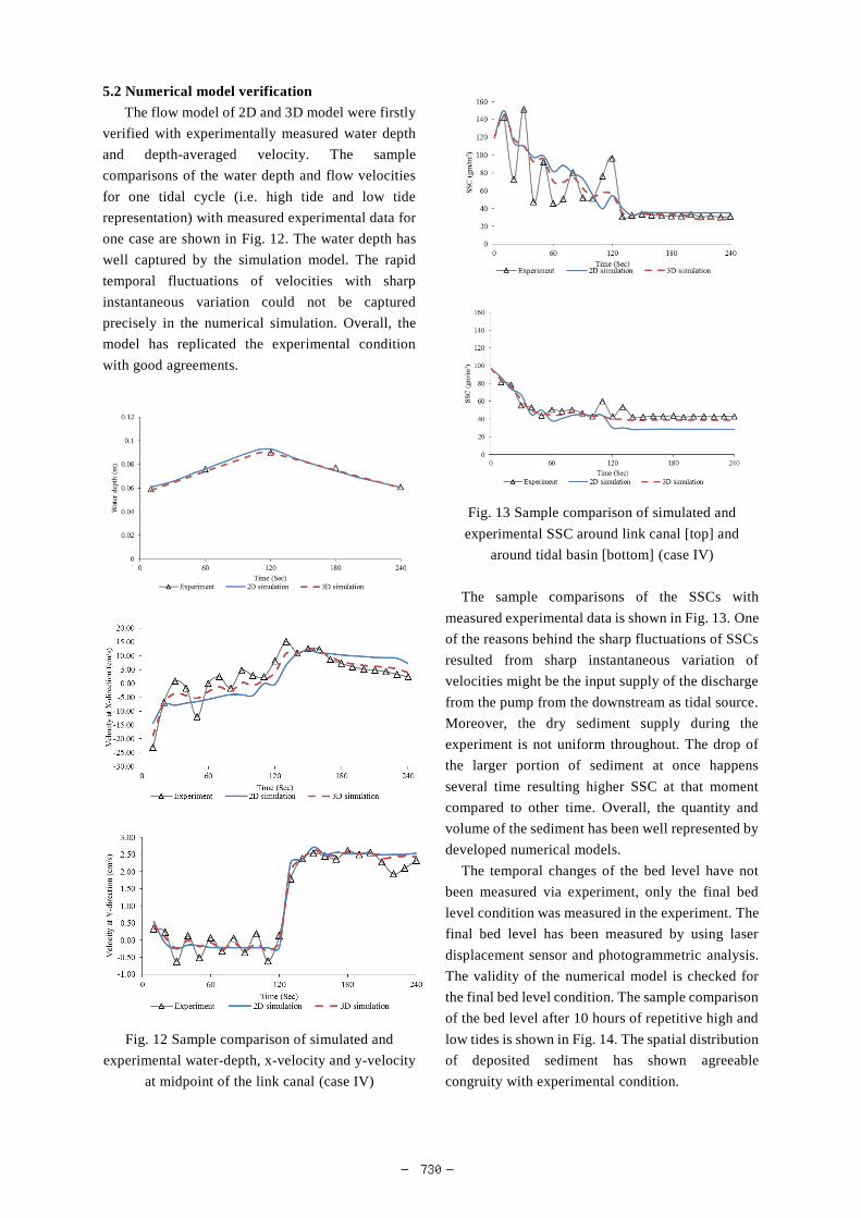
5.2 Numerical model verification

The flow model of 2D and 3D model were firstly

verified with experimentally measured water depth

and depth-averaged velocity. The sample

comparisons of the water depth and flow velocities

for one tidal cycle (i.e. high tide and low tide

representation) with measured experimental data for

one case are shown in Fig. 12. The water depth has

well captured by the simulation model. The rapid

temporal fluctuations of velocities with sharp

instantaneous variation could not be captured

precisely in the numerical simulation. Overall, the

model has replicated the experimental condition

with good agreements.

Fig. 12 Sample comparison of simulated and

experimental water-depth, x-velocity and y-velocity

at midpoint of the link canal (case IV)

Fig. 13 Sample comparison of simulated and

experimental SSC around link canal [top] and

around tidal basin [bottom] (case IV)

The sample comparisons of the SSCs with

measured experimental data is shown in Fig. 13. One

of the reasons behind the sharp fluctuations of SSCs

resulted from sharp instantaneous variation of

velocities might be the input supply of the discharge

from the pump from the downstream as tidal source.

Moreover, the dry sediment supply during the

experiment is not uniform throughout. The drop of

the larger portion of sediment at once happens

several time resulting higher SSC at that moment

compared to other time. Overall, the quantity and

volume of the sediment has been well represented by

developed numerical models.

The temporal changes of the bed level have not

been measured via experiment, only the final bed

level condition was measured in the experiment. The

final bed level has been measured by using laser

displacement sensor and photogrammetric analysis.

The validity of the numerical model is checked for

the final bed level condition. The sample comparison

of the bed level after 10 hours of repetitive high and

low tides is shown in Fig. 14. The spatial distribution

of deposited sediment has shown agreeable

congruity with experimental condition.

― 730 ―

2D simulation Experiment

Fig. 14 Sample comparison of simulated and

experimental bed level (case IV)

Table 1 Statistical comparison of experimental and

simulated results

The comparison of the flow velocity, SSC and

sediment deposition for all four cases has been

tabulated in Table 1. The table illustrates statistical

check using Percent Bias (to measure average

tendency of the simulated data to be larger or smaller

than their observed data) and Coefficient of

Determination (to describe the degree of collinearity

between simulated and measured data) of the

parameters (water depth, magnitude of the velocity,

SSC and deposition height) for all four cases with

agreeable indication.

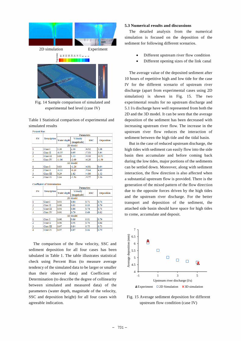
5.3 Numerical results and discussions

The detailed analysis from the numerical

simulation is focused on the deposition of the

sediment for following different scenarios.

Different upstream river flow condition

Different opening sizes of the link canal

The average value of the deposited sediment after

10 hours of repetitive high and low tide for the case

IV for the different scenario of upstream river

discharge (apart from experimental cases using 2D

simulation) is shown in Fig. 15. The two

experimental results for no upstream discharge and

5.1 l/s discharge have well represented from both the

2D and the 3D model. It can be seen that the average

deposition of the sediment has been decreased with

increasing upstream river flow. The increase in the

upstream river flow reduces the interaction of

sediment between the high tide and the tidal basin.

But in the case of reduced upstream discharge, the

high tides with sediment can easily flow into the side

basin then accumulate and before coming back

during the low tides, major portions of the sediments

can be settled down. Moreover, along with sediment

interaction, the flow direction is also affected when

a substantial upstream flow is provided. There is the

generation of the mixed pattern of the flow direction

due to the opposite forces driven by the high tides

and the upstream river discharge. For the better

transport and deposition of the sediment, the

attached side basin should have space for high tides

to come, accumulate and deposit.

Fig. 15 Average sediment deposition for different

upstream flow condition (case IV)

4

4.5

5

5.5

6

6.5

7

-1 1 3 5

Aver

age

dep

osi

tion

(m

m)

Upstream river discharge (l/s)

Experiment 2D Simulation 3D simulation

― 731 ―

If there is significant upstream flow, then that

space is reduced. Moreover, during the low tides also,

that space is not completely emptied which

ultimately reduces the effectiveness of the process.

In real case also, the transported and deposited

sediment during monsoon period is comparatively

lower than a drier period. During monsoon period,

due to the rainfall, the tidal basin is inundated to

some level and the flow of the river upstream is also

substantial. In such scenario, the sediment exchange

could not happen from the river to the tidal basin.

Furthermore, during the monsoon, the river carries a

great quantity of sediment with it so it cannot erode

the river bed material. Normally, the crossing dam is

constructed during the drier period and low flow

period. Diversion of the upstream flow is made so

that around the immediate upstream of the crossing

dam, artificial inundation would not happen. When

the river flow starts increasing from the pre-

monsoon period, the crossing dam is required to be

detached.

Similarly, the average value of the sediment

deposition is attempted to explore with the opening

size (shown in Fig. 16). The result shows there is not

a well-established relation. It shows it has a tendency

to deposit more sediment with increasing opening

size of the link canal. The spatial distribution of the

sediment is very much important for the sustainable

sediment deposition process to happen. If the

deposited sediment is more pronounced on the

entrance of the link canal, slowly, the rate of

transport and deposition of the sediment gets

reduced.

Fig. 16 Average sediment deposition for different

opening sizes of the link canal

The results shown in Fig. 16 does not provide the

idea about the spatial distribution. The simulation

results depict the good agreement with the

experimental condition except for the case II. In case

II, the experimental result is a little bit higher than

the simulated result. One of the reasons behind this

may be during the experiment, the repetition of same

hydraulic conditions of high tides and low tides may

not be acquired.

The experimental domain is limited. As

mentioned in the earlier chapter, due to the limited

size of the attached side basin, the wall effects are

clearly seen. The total or average sediment

deposition on attached side basin may not

completely provide reliable information in such

limitation. As supported by the experimental result

of the spatial distribution of the deposited sediment,

the two cases with narrower opening cases (case III

and case IV) showed the better effective TBM

process, the numerically simulated result in those

cases and other narrower opening cases are needed

to examine further. The nature of the spatial

distribution of the narrower opening cases (10 cm –

40 cm opening size) after 2 hours of the repetitive

experimental conditions is shown in Fig. 17. With

increasing the size of the opening size of the link

canal, more sediment is likely to get deposited in the

course of the link canal. In the case of Fig. 17 (a) and

(b), the opening size is very narrow as a result of

which, the flow velocity is high with high shear

stress.

Fig. 17 Spatial distribution of the deposited

sediment around the link canal for different opening

sizes after 2 hour of the repetitive high and low

tides (a: 10 cm, b: 20 cm, c: 30 cm and d: 40 cm)

4

4.1

4.2

4.3

4.4

4.5

4.6

4.7

4.8

4.9

5

0.00 1.00 2.00 3.00

Aver

age

dep

osi

tion

(m

m)

Ratio (Width of Link Canal / River Width)

Experiment 2D simulation 3D simulation

Case IV Case III

Case II Case I

― 732 ―

Within the main flow direction, the deposition of

the sediment doesn’t happen. In the case of Fig. 17

(c) and (d), the spatial extent of the deposition is

comparatively higher. If the provided case for the

river is in equilibrium, the recommended size of the

link canal if oriented in the proper direction is nearly

equal to the river width. The Fig. 17 (c) depicts the

ratio of the link canal width to the river width nearly

1.

The area near the wall of the link canal towards

the tidal source has developed a complex vortex- like

flow during the experiment which has a basically

higher value of shear stress that erodes the sediment

on that pocket. Such process is seen in all

experimental cases and even in wider opening cases

(shown in Photo 1). Fig. 18 shows the flow direction

of the 3D simulation in the wider case (i.e. case 1).

The flow directions and stream line directions show

that the pocket is always hit with the higher velocity

during the low tide. The water coming out from the

side basin hits directly on that pocket.

Photo 1 Typical erosion around the wall resulted by

vortex like flow (case I)

Fig. 18 Typical velocity distribution around the link

canal at low tide (case I)

Even in the wider link canal area, that pocket is

prone to erosion. In real case also, it happens which

tried to erode the bed and bank material in that

pocket. To protect from further scouring, concrete

blocks are used.

6. Conclusions

Four cases of the experiments with different

opening sizes of the link canal varying from 0.7

times the river width to thrice the river width were

performed. With the supply of discharge from the

downstream of the river as high tide and allowing to

go back as low tide, the experiments were conducted

to assess the effectiveness of TBM process. The

present work discussed in the experiment is

numerically simulated which shows quite good

agreement for the water level, velocity, SSC and

sediment deposition. The instantaneous peak

fluctuation of the parameters could not be simulated

but the overall value has been represented by both

the 2D and the 3D numerical model. Even the

developed model has not replicated the precise bed

form (ripple-like structure), the overall spatial and

temporal distribution of the deposited sediment has

been replicated in an agreeable way. The 3D model

has captured better replication than the 2D model.

Since the 3D model takes a huge computation time,

the 2D model has been used to explore different

scenarios in experimental domain.

The limitations due to which lots of set of

experimental investigations could not be done were

satisfied by running the different simulations using

2D model. The developed model can be applied to

simulate for the exploration of the best location of

the single /multiple link canals. For the detailed

physical mechanism in some local areas, the 3D

model can be used to explore the spatio–temporal

variation.

For the effective operation of TBM, the upstream

discharge should be diverted and crossing dam

should be constructed to create reduced upstream

discharge condition and to allow natural tidal

movement in selected tidal basin. Moreover, the

opening size of the link canal more or less equal to

the river width in equilibrium condition is

recommended. In the real case, if the natural river is

not intervened by human interactions and civil

― 733 ―

structures, the recommended size of the link canal is

more or less equal to the natural width of the river.

The experiment carried out is a preliminary stage

of TBM process replication with a simple approach

and it has many limitations. The research findings

would be utilized in the field of sediment

management. The study is focused on the land

heightening of the selected tidal basin and increasing

the river navigability to solve drainage congestion.

The next plan is to simulate TBM process

numerically real field data of Bangladesh which is

currently in progress. East beel Khuksia is taken as

the case study area after the field visit around the SW

region of Bangladesh. The fusion of utilization of

natural tide movement with some level of

engineering works and dredging/excavation of

deposited sediment around the entrance of the link

canal would strongly provide better results.

Acknowledgements

The research is supported by JST/JICA

SATREPS program on disaster

prevention/mitigation measures against floods and

storm surges in Bangladesh (PI: Dr. Hajime

Nakagawa). The first author is pleased to

acknowledge a Monbukagakusho scholarship. The

authors would also express their sincere thanks to Dr.

Masakazu Hashimoto for his co-operation during the

development of numerical model.

References

Akai K, Ueda S, Sawai K (1990): Sedimentation and

purification of water quality by tide in the water

course with marine basins. Techno-Ocean’ 90

international symposium. Kobe, Japan.

Ashida K, Michiue M (1972): Studies on bed load

transportation for nonuniform sediment and river

bed variation. Annuals of the Disaster Prevention

Resesearch Institute, Kyoto University 14(B): pp.

259–273.

Banglapedia (2012): Banglapedia - the National

Encyclopedia of Bangladesh.

Engelund F, Fredsøe J (1976): A Sediment Transport

Model for Straigth Alluvial Channels. Nordic

Hydrology 7: pp. 293–306.

Haque KNH, Chowdhury FA, Khatun KR (2015):

Participatory environmental governance and

climate change adaptation: mainstreaming of tidal

river management in south-west Bangladesh. In:

Ha H (ed) Land and Disaster Management

Strategies in Asia, pp. 189–208.

Hashimoto M, Kawaike K, Nakagawa H, Yoneyama

N (2016): Assessing the pollutant spreading using

a flood simulation model in Dhaka city,

Bangladesh. IAHR APD 2016.

Hume TM, Herdendorf C (1993): On the use of

empirical stability relationships for characterising

estuaries. J. Coastal Research 9: pp. 413–422.

Ibne Amir MSI, Khan MSA, Kamal Khan MM,

Golam Rasul M, Akram F (2013): Tidal river

sediment management - a case study in

southwestern Bangladesh. International Journal

of Civil Science and Engineering 7(3).

Islam N (2001): The open approach to flood control:

The way to the future in Bangladesh. Futures

33(8–9): pp. 783–802. DOI: 10.1016/S0016-

3287(01)00019-2.

Iwagaki Y (1956): Fundamental study on critical

tractive force. Tans. JSCE 41: pp. 1–21.

Jarrett JT (1976): Tidal Prism - Inlet Area

Relationships. Department of Army Corps of

Engineers.

Khadim FK, Kar KK, Halder PK, Rahman MA,

Morshed AKMM (2013): Integrated Water

Resources Management (IWRM) Impacts in South

West Coastal Zone of Bangladesh and Fact-

Finding on Tidal River Management (TRM).

Journal of Water Resource and Protection 5(10):

pp. 953–961. DOI: 10.4236/jwarp.2013.510098.

Kibria Z (2011): Tidal River Management (TRM)

Climate Change Adaptation and Community

Based River Basin Management and in Southwest

Coastal Region of Bangladesh. Uttaran: Dhaka.

Kraus NC (1998): Inlet cross-section area calculated

by process-based model. International Conference

on Coastal Engineering. ASCE. Reston, VA, pp.

3265—3278.

LeConte LJ (1905): Notes on the improvement of

river and harbor outlets in the US. Trans. ASCE :

Discussion Paper 55(Dec): pp. 306–308.

Menter FR, Ferreira JC, Esch T (2003): The SST

Turbulence Model with Improved Wall Treatment

for Heat Transfer Predictions in Gas Turbines.

International Gas Turbine Congress 2003 (1992):

― 734 ―

pp. 1–7.

Nezu I, Nakagawa H (1993): Turbulence in open-

channel flows. IAHR Monograph. A. A. Balkema:

Rotterdam, The Netherlands.

Nielsen P (1992): Coastal bottom boundary layers

and sediment transport. Advanced Series on

Ocean Engineering. World Scientific.

Nowreen S, Jalal MR, Khan MSA (2014): Historical

analysis of rationalizing South West coastal

polders of Bangladesh. Water Policy 16(2): pp.

264–279. DOI: 10.2166/wp.2013.172.

O’Brien MP (1931): Estuary Tidal Prism Related to

Entrance Areas. Civil Engineering 1(8): pp. 738-

739.

O’Brien MP (1969): Equilibrium flow areas of tidal

inlets on sandy coasts. J. Waterw. Harb. Div.

WW1: pp. 43–52. DOI: 10.9753/icce.v10.25p.

Ogawa Y, Sawai K (2013): Estuary sedimentation

control using a tidal reservoir. Advances in River

Sediment Research. CRC Press pp. 1417–1424.

OpenCFD Ltd. (2009a): User Guide. OpenFOAM,

The Open Source CFD Toolbox.

OpenCFD Ltd. (2009b): Programmer’s Guide.

OpenFOAM, The Open Source CFD Toolbox.

Ota K, Sato T, Nakagawa H, Kawaike K (2016):

Three-Dimensional Simulation of Local Scour

around a Weir-Type Structure: Hybrid Euler-

Lagrange Model for Bed-Material Load. Journal

of Hydraulic Engineering 143(4): 4016096. DOI:

10.1061/(ASCE)HY.1943-7900.0001263.

Paul A, Nath B, Abbas MR (2013): Tidal River

Management (TRM) and its implication in disaster

management : A geospatial study on Hari-Teka

river basin , Jessore ,. International Journal of

Geomatics and Geosciencse 4(1): pp. 125–135.

Powell MA, Thieke RJ, Mehta AJ (2006):

Morphodynamic relataionships for ebb and flood

delta volumes at Florida’s entrances. Ocean

Dynamics 56: pp. 295–307.

Rahman MZ, Islam MS, Khan ZH (2015): Tidal

River Management (TRM)-An Innovative

Scientific Approach for Sustainable Sediment

Management. international Conference on Recent

Innovation in Civil Engineering for Sustainable

Development (IICSD-2015), pp. 954–959.

Rahman R, Salehin M (2013): Flood Risks and

Reduction Approaches in Bangladesh. In: Shaw R,

Mallick F and Islam A (eds) Disaster Risk

Reduction Approaches in Bangladesh. Springer

Japan: Tokyo, pp. 65-90.

Rakhorst RD (2007): Delft University of Technology.

Delft University of Technology.

Rezaie AM, Naveram UK (2013): Tidal river

management : An innovative approach for

terminating drainage congestion and raising land

through sedimentation in the Bhabodaho area ,

Bangladesh. Advances in River Sediment Research.

CRC Press, pp. 1363–1375.

Richardson JF, Zaki WN (1954): Sedimentation and

fluidization; part I. Transactions of the Institution

of Chemical Engineers 32: pp. 35–53.

Rubey WW (1933): Settling velocity of gravel, sand,

and silt particles. American Journal of Science, pp.

325–338. DOI: 10.2475/ajs.s5-25.148.325.

Shampa, Pramanik MIM (2012): Tidal River

Management (TRM) for Selected Coastal Area of

Bangladesh to Mitigate Drainage Congestion.

International Journal of Scientific & Technology

Research 1(5): pp. 1–6.

Soulsby RL, Damgaard JS (2005): Bedload sediment

transport in coastal waters. Coastal Engineering

52(8): pp. 673–689. DOI:

10.1016/j.coastaleng.2005.04.003.

Staveren MF Van, Warner JF, Khan MSA (2017):

Bringing in the tides. From closing down to

opening up delta polders via Tidal River

Management in the southwest delta of Bangladesh.

Water Policy 19: pp. 147–164. DOI:

10.2166/wp.2016.029.

Stive MJF, Rakhorst RD (2008): Review of

empirical relationships between inlet cross-section

and tidal prism. Journal of Water Resources and

Environmental Engineering 23(23): pp. 89–95.

Talchabhadel R, Nakagawa H, Kawaike K (2016a):

Tidal River Management ( TRM ) and Tidal Basin

Management ( TBM ): A case study on Bangladesh.

FLOODrisk 2016 - 3rd European Conference on

Flood Risk Management, pp. 1–7. DOI:

10.1051/e3sconf/201 60712009.

Talchabhadel R, Nakagawa H, Kawaike K (2016b):

Experimental study on suspended sediment

transport to represent Tidal Basin Management.

Journal of Japanese Society of Civil Engineers,

Ser B1 (Hydraulic Engineering) 60: pp. 847–852.

Talchabhadel R, Nakagawa H, Kawaike K (2016c):

Experimental Study on Transportation of

― 735 ―

Suspended Sediment on Side Basin. Annuals of the

Disaster Prevention Resesearch Institute, Kyoto

University 59(B): pp. 411–419.

Talchabhadel R, Nakagawa H, Kawaike K,

Hashimoto M, Sahboun N (2017a): Experimental

investigation on opening size of tidal basin

management: a case study in southwestern

Bangladesh. Journal of Japanese Society of Civil

Engineers, Ser B1 (Hydraulic Engineering) 61: pp.

781–786.

Talchabhadel R, Nakagawa H, Kawaike K, Sahboun

N (2017b): Experimental study on Tidal Basin

Management : A case study of Bangladesh. E-

proceedings of the 37th IAHR World Congress.

Tutu A (2005): River Management in Bangladesh: A

People’s Initiative to Solve Water-Logging.

Participatory Learning and Action 15(April): pp.

117–123.

Ullah MW, Mahmud S (2017): Appropriate planning,

design and implementation modalities for

successful application of Tidal River Management

(TRM) in coastal delta. 6th International

Conference on Flood Management (ICWFM-

2017), pp. 133–140.

Van de Kreeke J, Haring J (1980): Stability of

Estuary Mouths in the Rhine-Meuse Delta.

International Conference on Coastal Engineering,

ASCE. NY, pp. 2627–2639.

Van Rijn LC (1984a): Sediment transport, part II:

Suspended-load transport. Journal of Hydraulic

Engineering, ASCE 110(11): pp. 1613–1641.

Van Rijn LC (1984b): Sediment transport - part III:

Bed forms and alluvial roughness. Journal of

Hydraulic Division, ASCE 110(12): pp. 1733–

1754.

Wu W, Wang SSY (2006): Formulas for Sediment

Porosity and Settling Velocity. Journa of

Hydraulic Egineering 132(8): pp. 852–862. DOI:

10.1061/(ASCE)0733-9429(2006)132:8(858)

(Received June 13, 2017)

― 736 ―