Experimental chaotic quantification in bistable vortex inducedvibration systems
B.H. Huynha, T. Tjahjowidodob,⁎
a Energy Research Institute at NTU, Interdisciplinary Graduate School, Nanyang Technological University, Singapore 639798, Singaporeb School of Mechanical & Aerospace Engineering, Nanyang Technological University, Singapore 639798, Singapore
A R T I C L E I N F O
Keywords:Vortex induced vibrations (VIV)Bistable stiffnessChaotic vibrationsLyapunov exponentSurrogate data testing
A B S T R A C T
The study of energy harvesting by means of vortex induced vibration systems has been initiated afew years ago and it is considered to be potential as a low water current energy source. Theenergy harvester is realized by exposing an elastically supported blunt structure under waterflow. However, it is realized that the system will only perform at a limited operating range (waterflow) that is attributed to the resonance phenomenon that occurs only at a frequency thatcorresponds to the fluid flow. An introduction of nonlinear elements seems to be a prominentsolution to overcome the problem. Among many nonlinear elements, a bistable spring is knownto be able to improve the harvested power by a vortex induced vibrations (VIV) based energyconverter at the low velocity water flows. However, it is also observed that chaotic vibrations willoccur at different operating ranges that will erratically diminish the harvested power and cause adifficulty in controlling the system that is due to the unpredictability in motions of the VIVstructure. In order to design a bistable VIV energy converter with improved harvested power andminimum negative effect of chaotic vibrations, the bifurcation map of the system for varyinggoverning parameters is highly on demand.
In this study, chaotic vibrations of a VIV energy converter enhanced by a bistable stiffnesselement are quantified in a wide range of the governing parameters, i.e. damping and bistablegap. Chaotic vibrations of the bistable VIV energy converter are simulated by utilization of awake oscillator model and quantified based on the calculation of the Lyapunov exponent.Ultimately, a series of experiments of the system in a water tunnel, facilitated by a computer-based force-feedback testing platform, is carried out to validate the existence of chaoticresponses. The main challenge in dealing with experimental data is in distinguishing chaoticresponse from noise-contaminated periodic responses as noise will smear out the regularity ofperiodic responses. For this purpose, a surrogate data test is used in order to check thehypotheses for the presence of chaotic behavior. The analyses from the experimental resultssupport the hypothesis from simulation that chaotic response is likely occur on the real system.
1. Introduction
Vortex induced vibrations of elastically constrained structures in water flows have recently received intensive attentions as apromising and potential alternative among many available sources of renewable energy. The first vortex-induced-vibrations basedenergy converter trademarked as VIVACE was introduced in [1]. The VIVACE energy converter consists of a cylinder submerged
http://dx.doi.org/10.1016/j.ymssp.2016.09.025Received 27 April 2016; Received in revised form 8 August 2016; Accepted 17 September 2016
⁎ Corresponding author.E-mail address: [email protected] (T. Tjahjowidodo).
Mechanical Systems and Signal Processing 85 (2017) 1005–1019
perpendicularly into a water flow. The cylinder is elastically supported by a linear spring and its motion is constrained along thecross-flow direction, thus allowing it to move in one degree of freedom. When the water flow passes the cylinder, it will induceperiodic drag and lift forces imposing along the surface of the cylinder that is due to the occurrence of vortices alternately sheddingon two sides of the wake region behind the cylinder. Under the effect of lift forces, the cylinder will vibrate in the cross-flow directionsince it is constrained by the spring in this direction. These vibrations of the cylinder are known as VIV (vortex induced vibrations),whose elaborative characteristics are widely reviewed in ([2–4]). A transmission mechanism is utilized to connect the cylinder to agenerator and convert the VIV into rotations of the shaft in the generator. In this way, usable energy, i.e. electrical energy, isproduced from kinetic energy of water flows.
A critical parameter in designing a VIV energy converter is its natural frequency, which essentially is determined by the springstiffness and the effective mass of the oscillating structure. In order to maximize the harvested power, the natural frequency of thesystem must coincide with the exciting frequency of lift forces, which is determined by velocity of the water flow. This resonancerequirement will allow the VIV energy converter to be designed effectively for specific water flow conditions. This outstanding meritmakes this approach for energy harvesting potential and promising. Unfortunately, another issue arises for a VIV energy converteroperating in practical scenario, where water flow velocity in nature typically fluctuates severely. When the flow velocity deviates farfrom the resonance frequency, the effectiveness of the energy converter will drop significantly. Since this adversity was revealed,there were several theoretical and experimental studies (e.g. [5–10]), which focused on characterizing and optimizing the designingparameters of a VIV energy converter through maximizing the resonance range and increasing vibrating amplitude. The parametersinclude mass, damping, stiffness and surface roughness of the vibrating structure.
Among those studies, the significantly positive effect from the approach of appending a nonlinear stiffness element to the systemin order to broaden the resonance range is discussed. Experimental studies in [11] and [12] have shown that a VIV energy converterwith a hardening stiffness element has widened the resonance range toward the high operating working frequencies, i.e. high speedwater flows. In contrast, a bistable stiffness element is capable to improve the harvested power at low operating frequencies ([13]). Anumerical analysis, which will be discussed in details later in Section 2, also shows that bistable stiffness can significantly improveharvested power from a VIV energy converter at low velocity water flows. However, when parameters vary, including the water flowvelocity, the harvested power might drop drastically due to the chaotic behavior that might manifest itself in the vibration response.Chaotic signal is defined as a non-periodic, unpredictable and seemingly noisy vibration [14]. It might manifest themselves in anynonlinear mechanical systems and commonly it appears in those with severe nonlinearities, such as mechanical systems withbacklash ([15–17]) or those with hysteresis ([18–20]).
Chaotic vibrations are evidently undesired for the operation of a VIV energy converter because of the low harvested power andthe unpredictability in motions that will result in difficulties in controlling the system. For this reason, the feasibility in application ofbistable stiffness in a VIV energy converter to improve its performance requires a design for the converter that can avoid chaoticvibrations from its operating range. The prerequisite to design such a converter is the knowledge of chaotic response dependency tothe governing parameters of the system.
Zhao et al. [21] studied chaotic responses of a VIV structure in laboratory scale. Initially, they measured the state variables of thesystem, i.e. the output displacement and lift force, on a testing apparatus. Subsequently, they confirmed the existence of chaoticvibration by prescribing the recorded displacement on a position-controlled-testing-platform and measured the lift forces. From theobservation, they concluded the existence of chaotic vibrations when large discrepancies occur between the two measured lift forces.Perdikaris et al. [22] studied vibrations on a VIV system in a constant flow for varying amplitudes and fixed frequency. Theyobserved that chaotic vibration manifests itself in a case of moderate amplitudes and confirmed the chaotic phenomenon byanalyzing the frequency spectrum of the lift force, where no dominant frequency appears in the spectrum. Blackburn and Henderson[23] used the 2D numerical simulation to investigate the lock-in behavior of the cylinder excited by a constant flow. They confirmedchaotic vibrations at a certain frequency ratio by observing non-periodic vibrations and the auto-spectrum of the cross-flowvibrations, where the spectral peaks do not match to the natural frequency and the Strouhal frequency.
In this paper, chaotic vibrations of a bistable VIV energy converter will be quantified in a wide range of the two governingparameters: damping and bistable gap, which are figured out by a dimensional analysis on the system. The quantification will bemainly based on the largest Lyapunov exponent of the time series displacement of the cylinder, which can be considered as thefootprint of chaos if it is positive and its magnitude measures the degree of chaos in the system ([24]). Therefore, its dependency ondamping and bistable gap will serve as a guideline to design a bistable VIV energy converter.
The calculation of the largest Lyapunov exponent relies on the nonlinear time series analysis procedure, which is systematicallypresented in [25–27] and was successfully applied to analyze the chaotic responses of some mechanical systems in [15] and [28]. Toevaluate, a time delay phase space is reconstructed from the time series data to calculate the largest Lyapunov exponent. In addition,dealing with experimental data requires a procedure to distinguish the presence of chaotic behavior in the non-linear system and ofthe linearly correlated noise and the surrogate data testing will be carried out to perform this task. This approach offers a moreconsistent chaotic quantifier and is capable of assessing the chaotic phenomenon from a single data set.
The paper is organized as follows: In Section 2, the wake oscillator model that is utilized to simulate the time series displacementof the structure will be presented. The expression of a bistable stiffness element applied in the VIV energy converter and the effect ofbistable stiffness on performance of a VIV energy converter will also be discussed in this section. Elaborative discussion on theprocedure of reconstructing the time delay phase space and calculating the largest Lyapunov exponent as well as results from thisprocedure can be found in Section 3. While Section 3 mainly discusses the analysis on simulated data, Section 4 presents theexperimental setup of a bistable VIV system in a real water tunnel, data analysis and implementation the surrogate data testing toverify the presence of chaotic responses. Some key conclusions from this study are drawn in Section 5.
B.H. Huynh, T. Tjahjowidodo Mechanical Systems and Signal Processing 85 (2017) 1005–1019
1006
2. Background
This section concentrates on the numerical simulation of vortex induced vibration systems utilizing the wake oscillator model.The discussion comprises the dynamic modeling of the system with bistable springs, dimensional analysis of the nonlinear system, abrief comparison on the performance of the VIV system with linear and bistable spring and a particular case when the nonlinearsystem results in chaotic behavior.
2.1. VIV modeling by wake oscillator model
For simulation purposes, the VIV system is modeled as shown in Fig. 1. The system consists of a cylinder, as the oscillating bluntobject, with an effective mass of m, diameter of D and length of L. Referring to Fig. 1, the cylinder length is oriented along the z-direction and is submerged in a water stream along x-direction with a constant flow velocity of U. The cylinder is supported by alinear spring with a stiffness constant of k, and is constrained in such it can only vibrate in y-direction. The effective mass and thestiffness value determine the natural frequency of the system; thus, will also define the resonance phenomenon that corresponds tothe vortex shedding frequency from the water flow. The structural damping, c, that comprises the damping from the mechanicalstructure and that from the PTO (power take-off) box, will define the resonance range (please note that the harvested power, fromanalytical point of view, will be considered to be proportional to the damping from the PTO). In particular, Khalak and Williamson([29–31]) reported the mass ratio, m*, which represents the ratio between the effective mass and the fluid mass displaced by thecylinder, will also determine the resonance range..
To dynamically simulate the system, the wake oscillator model, which was proposed in [32], modified and validated in [33], isutilized. In this model, the dynamic equation of the VIV structure (Eq. 1) is coupled with the nonlinear wake oscillator equation (Eq.2) to simulate the waking effect of the vortex shedding in the corresponding vortex-induced-vibration system.
mY rY hY S q + + = ( ) (1)
q ε πSt U D βq λq q πSt U D q F Y + [2 ( / )](1 − + ) + [2 ( / )] = ( )2 4 2 (2)
where:
1. m: sum effective mass and fluid added – mass2. r: sum of structural damping and fluid added – damping3. h: spring stiffness4. Y: displacement of cylinder in cross-flow direction5. S(q): vortex shedding force6. q: wake variable7. St: Strouhal number8. U: water flow velocity9. D: diameter of cylinder
10. F(Y ): effect from vibrations of the structure on the wake11. ε, β, λ: coefficients of nonlinearity (refer to [32] and [33] for detailed explanations)
Fig. 1. Model of a VIV energy converter.
B.H. Huynh, T. Tjahjowidodo Mechanical Systems and Signal Processing 85 (2017) 1005–1019
1007
2.2. Bistable stiffness modeling and dimensional analysis
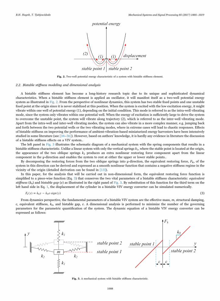
A bistable stiffness element has become a long-history research topic due to its unique and sophisticated dynamicalcharacteristics. When a bistable stiffness element is applied an oscillator, it will manifest itself as a two-well potential energysystem as illustrated in Fig. 2. From the perspective of nonlinear dynamics, this system has two stable fixed points and one unstablefixed point at the origin since it is never stabilized at this position. When the system is excited with the low excitation energy, it mightvibrate within one well of potential energy (1), depending on the initial condition. This mode is referred to as the intra-well vibratingmode, since the system only vibrates within one potential well. When the energy of excitation is sufficiently large to drive the systemto overcome the unstable point, the system will vibrate along trajectory (2), which is referred to as the inter-well vibrating mode.Apart from the intra-well and inter-well vibrating modes, the system can also vibrate in a more complex manner, e.g. jumping backand forth between the two potential wells or the two vibrating modes, where in extreme cases will lead to chaotic responses. Effectsof bistable stiffness on improving the performance of ambient-vibration-based miniaturized energy harvesters have been intensivelystudied in some literature (see [34–36]). However, based on authors’ knowledge, it is hardly any evidence in literature the discussionof a bistable stiffness effects on a VIV system..
The left panel in Fig. 3 illustrates the schematic diagram of a mechanical system with the spring components that results in abistable stiffness characteristic. Unlike a linear system with only the vertical springs k1, where the stable point is located at the origin,the appearance of the two oblique springs k2 produces an extra nonlinear restoring force component apart from the linearcomponent in the y-direction and enables the system to rest at either the upper or lower stable points..
By decomposing the restoring forces from the two oblique springs into y-direction, the equivalent restoring force, Fk, of thesystem in this direction can be derived and expressed as a smooth nonlinear function that contains a negative stiffness regime in thevicinity of the origin (detailed derivation can be found in [13]).
In this paper, for the analysis that will be carried out in non-dimensional form, the equivalent restoring force function issimplified to a piece-wise function (Eq. 3) that conserves the two vital parameters of a bistable stiffness characteristic: equivalentstiffness (k0) and bistable gap (ε) as illustrated in the right panel of Fig. 3. By substitution of this function for the third term on theleft hand side in Eq. 1, the displacement of the cylinder in a bistable VIV energy converter can be simulated numerically.
F y k y k ε sign y( ) = − ⋅ ( )k 0 0 (3)
From dynamics perspective, the fundamental parameters of a bistable VIV system are the effective mass, m, structural damping,c, equivalent stiffness, k0, and bistable gap, ε. A dimensional analysis is performed to minimize the number of the governingparameters for the parametric quantification of the system. The dynamic equation of a bistable VIV energy converter can beexpressed as follows:
Fig. 2. Two-well potential energy characteristic of a system with bistable stiffness element.
Fig. 3. A mechanical system with bistable stiffness characteristic.
B.H. Huynh, T. Tjahjowidodo Mechanical Systems and Signal Processing 85 (2017) 1005–1019
1008
my cy F y F t + + ( ) = ( )k (4)
where F(t) represents the lift force exciting the cylinder as a function of time. It should be noted that Eq. (4) is equivalent to Eq. (1)that is represented in the wake oscillator model. Some non-dimensional parameters are introduced, namely p = y
ε , ω = km0
2 0 , t ω t= 0 ,
α = εD and ζ = c
k m2 0. By substituting these quantities to Eq. (4), its dimensionless form can be obtained as follow:
⎛⎝⎜
⎞⎠⎟p ζp F p γF t
ω" + 2 ′ + ( ) =k
0 (5)
where: F p p p( )= − sign( )k , γ =k ε10, p′ = dp
dtand p′′ = d p
dt
2
2 . The system turns out to be governed by two main parameters ζ and γ. It
should be noted that γ depends on k0 or ε. Since k0 and m determine the natural frequency of the system, ε (or α in its dimensionlessform), will be varied to investigate the effect of different γ.
Typical parameters of a VIV system presented in [31], i.e. m*=10.1 and ζ0=0.00129, will be utilized in this paper. The naturalfrequency of the system in water is selected to be fn, water=0.7 Hz and the equivalent stiffness, k0, is calculated accordingly based onthis preselected values. The diameter of the cylinder is chosen to be D=0.05 m to meet the dimension of the water tunnel utilized inthe experiment. All these parameters are applied to the coupling equations to simulate the displacement of the cylinder at differentwater flow velocity, U.
2.3. Effect of bistable stiffness on a VIV energy converter
Using the wake oscillator model, the harvested power can be estimated. The average vibrational power, P*, is calculated based onthe velocity of the vibrating structure, y . Fig. 4 shows the average vibrational power versus water flow velocity, U, from the bistablesystem with different bistable gap values and the linear system with the equivalent stiffness. It can be observed that the bistablespring exhibits a minor effect on the system with a small bistable gap (α=0.02). When the bistable gap is increased (α=0.2), theharvested power is strikingly improved at low speed water flows due to large amplitude vibrations in the inter-well vibrating mode.However, the power suddenly drops when water flow velocity is increased (beyond 0.175 m/s water velocity). From our observation,it is suspected that the drop in power is attributed to the chaotic vibrations that occur on corresponding water flow velocities..
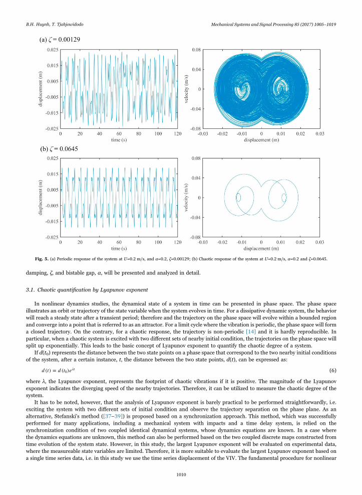
The occurrence of chaotic vibrations in a bistable VIV energy harvested also depends on the damping imposed to the system.Fig. 5 shows the vibrating response of the system when the damping value, ζ, is changed. In the upper panel of the figure (a), theresponse of the system is chaotic at a low value of damping, ζ=0.00129. However, when the damping is increased (ζ=0.0645), thechaotic effect diminishes and the system vibrates periodically (see Fig. 5b)..
Evidently, the bistable stiffness can only improve the harvested power when it is configured by a sufficiently large bistable gap.Unfortunately, increasing the bistable gap apparently is suspected to result in chaotic vibrations. Therefore, the negative effectcaused by chaotic vibrations must be taken into account when one wants to apply bistable stiffness to improve harvested power of aVIV energy converter. Besides, imposing a high amount of damping to the system seems to be able to control the chaotic vibrationsof the bistable VIV energy converter. To confirm these observations, hereafter, the study will focus on parametrically quantifyingchaotic vibrations of a bistable VIV energy converter to map the occurrence of chaotic response as a function of the governingparameters α and ζ.
3. Parametric quantification of chaotic vibrations
At this stage, however, it is not certain yet that the suspected chaotic responses are, indeed, chaotic. Therefore, in this section,first, we will discuss some theoretical analysis to quantify the chaotic degree on a response. Lyapunov exponent, which is consideredas a credible tool to quantify the chaotic degree in a time series data, will be discussed including the detailed procedure forestimation the quantifier. In the last part of this section, the Lyapunov exponent map of the bistable VIV energy converter for varying
Fig. 4. Vibrational power versus water flow velocity from a bistable system with different bistable gap values and a linear system with the equivalent stiffness.
B.H. Huynh, T. Tjahjowidodo Mechanical Systems and Signal Processing 85 (2017) 1005–1019
1009
damping, ζ, and bistable gap, α, will be presented and analyzed in detail.
3.1. Chaotic quantification by Lyapunov exponent
In nonlinear dynamics studies, the dynamical state of a system in time can be presented in phase space. The phase spaceillustrates an orbit or trajectory of the state variable when the system evolves in time. For a dissipative dynamic system, the behaviorwill reach a steady state after a transient period; therefore and the trajectory on the phase space will evolve within a bounded regionand converge into a point that is referred to as an attractor. For a limit cycle where the vibration is periodic, the phase space will forma closed trajectory. On the contrary, for a chaotic response, the trajectory is non-periodic [14] and it is hardly reproducible. Inparticular, when a chaotic system is excited with two different sets of nearby initial condition, the trajectories on the phase space willsplit up exponentially. This leads to the basic concept of Lyapunov exponent to quantify the chaotic degree of a system.
If d(t0) represents the distance between the two state points on a phase space that correspond to the two nearby initial conditionsof the system, after a certain instance, t, the distance between the two state points, d(t), can be expressed as:
d t d t e( ) = ( ) λt0 (6)
where λ, the Lyapunov exponent, represents the footprint of chaotic vibrations if it is positive. The magnitude of the Lyapunovexponent indicates the diverging speed of the nearby trajectories. Therefore, it can be utilized to measure the chaotic degree of thesystem.
It has to be noted, however, that the analysis of Lyapunov exponent is barely practical to be performed straightforwardly, i.e.exciting the system with two different sets of initial condition and observe the trajectory separation on the phase plane. As analternative, Stefanski's method ([37–39]) is proposed based on a synchronization approach. This method, which was successfullyperformed for many applications, including a mechanical system with impacts and a time delay system, is relied on thesynchronization condition of two coupled identical dynamical systems, whose dynamics equations are known. In a case wherethe dynamics equations are unknown, this method can also be performed based on the two coupled discrete maps constructed fromtime evolution of the system state. However, in this study, the largest Lyapunov exponent will be evaluated on experimental data,where the measureable state variables are limited. Therefore, it is more suitable to evaluate the largest Lyapunov exponent based ona single time series data, i.e. in this study we use the time series displacement of the VIV. The fundamental procedure for nonlinear
Fig. 5. (a) Periodic response of the system at U=0.2 m/s, and α=0.2, ζ=0.00129; (b) Chaotic response of the system at U=0.2 m/s, α=0.2 and ζ=0.0645.
B.H. Huynh, T. Tjahjowidodo Mechanical Systems and Signal Processing 85 (2017) 1005–1019
1010
time series analysis is discussed in [25–27]. To elaborate, from the single time series data, a time delay phase space, where theLyapunov spectrum of the system in the original phase space can be conserved, will be reconstructed. Then, the Lyapunov exponentis evaluated from the state points that are created by embedding the time series data to the reconstructed phase space.
3.2. Reconstruction of time delay phase space
In this study, the analysis is carried out on the time series data of the cylinder VIV displacement, y(t). When this time series isembedded to the time delay phase space, the state of the system at time t is represented in the following state vector:
y t y t y t t y t d t( ) = [ ( ), ( + ), ... , ( + ( − 1) )]d d (7)
where td is the time delay and d is the embedding dimension of the reconstructed phase space.
3.2.1. Selection of time delayThe phase space is reconstructed from the time series data, y(t), with time delay td. In order to analyze the chaotic behavior on
the response, the time delay has to be properly selected. The selection is based upon the minimization of the correlation in eachdimension of the phase space. Intuitively, auto-correlation technique will be able to serve for this task, however, it is suggested in[26], the average mutual information (AMI) is more appropriate when one deals with nonlinear system. The formulation of AMI fortime series S(t) is presented as follows:
where P(A,B) is the joint probability density for set A and B, and P(A) is the individual probability density for set A. Fig. 6 illustratesthe AMI of the time series displacement of the cylinder at U=0.175 m/s, ζ=0.00129 and α=0.25. It is suggested from the figure thatthe time delay, td, is chosen to be 0.369 s, as the AMI reaches its first local minimum at the corresponding time instance..
3.2.2. Selection of embedding dimensionAfter acquiring the time delay, the embedding dimension is selected to complete the phase space reconstruction. The embedding
dimension, d, determines the number of elements in a state vector, or the dimensionality of the reconstructed phase space. The basicidea for selection of the embedding dimension is that it must be sufficiently large so that the attractor revealed in the reconstructedphase space is totally unfolded. In this paper, the method proposed in [40] is applied to select the embedding dimension. Toelaborate the method, y(d) and y(d+1) are defined as the state vectors in the reconstructed phase space with the embeddingdimension d and d+1, respectively. The Euclidian distance between each point and its nearest neighbor in the embedding phasespace is calculated. Then, the ratio of this distance of the point y(d+1) to one of the point y(d) is defined as the embedding errorwhen the embedding dimension is increased from d to d+1. The quantity E(d) that measures the mean value of all the embeddingerrors of all the reference vector points is calculated. Finally, the selection of the embedding dimension is based on the ratio E1(d)defined as follows:
E d E d E d( ) = ( + 1)/ ( )1 (9)
E1(d) indicates the change of E(d) when the embedding dimension is increased from d to d+1.Dimension d0+1 is selected as the embedding dimension if E1(d) starts to saturate at a dimension d0. Fig. 7 illustrates the ratio
E1(d) as a function of the embedding dimension from the time series displacement of the VIV at U=0.175 m/s, ζ=0.00129 andα=0.25. This ratio saturates when the embedding dimension is larger than 3. Therefore, the embedding dimension d=4 is selected inthis case..
Fig. 6. AMI of the time series displacement of the cylinder at U=0.175 m/s, ζ=0.00129 and α=0.25.
B.H. Huynh, T. Tjahjowidodo Mechanical Systems and Signal Processing 85 (2017) 1005–1019
1011
3.3. Calculation of the Lyapunov exponent
After the time delay and the embedding dimension are evaluated, the phase space is subsequently reconstructed to allow for theLyapunov exponent calculation. The calculation relies on the direct method of the largest Lyapunov exponent estimation reviewed in[27]. The calculation is started by specifying a state point, y(t), at a specific time instance t, and afterwards the Euclidian distancebetween this point and its nearest neighbor is calculated. The distances between these two points are repeatedly evaluated, for everyperiod of Δt, while the points evolve in phase space. At the same time, the ratio between the evolving distance values and its originaldistance are recorded. Subsequently, the averaged ratio, which later is referred to as a prediction error is plotted against theevolution time, Δt, on logarithmic scale.
Intuitively, the plot represents the growth of the phase space trajectory and if it is exponentially growing, a linear function againstthe evolution time will be observed on the plot. In other word, a positive slope on the plot will indicate the exponential growth in thedistance of nearby trajectories, where the slope estimates the largest Lyapunov exponent that represents the chaotic degree of thetime series.
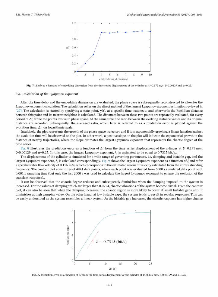
Fig. 8 illustrates the prediction error as a function of Δt from the time series displacement of the cylinder at U=0.175 m/s,ζ=0.00129 and α=0.25. In this case, the largest Lyapunov exponent, λ, is estimated to be equal to 0.7315 bit/s..
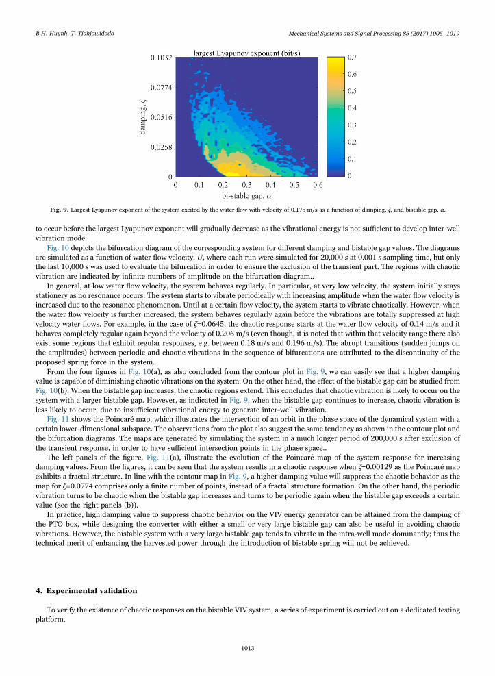
The displacement of the cylinder is simulated for a wide range of governing parameters, i.e. damping and bistable gap, and thelargest Lyapunov exponent, λ, is calculated correspondingly. Fig. 9 shows the largest Lyapunov exponent as a function of ζ and α fora specific water flow velocity of 0.175 m/s, which corresponds to the estimated resonant velocity calculated from the vortex sheddingfrequency. The contour plot constitutes of 4941 data points, where each point was evaluated from 5000 s simulated data point with0.001 s sampling time (but only the last 2000 s was used to calculate the largest Lyapunov exponent to ensure the exclusion of thetransient response)..
It can be observed that the chaotic degree reduces and subsequently diminishes when the damping imposed to the system isincreased. For the values of damping which are larger than 0.0774, chaotic vibrations of the system become trivial. From the contourplot, it can also be seen that when the damping increases, the chaotic region is more likely to occur at small bistable gaps until itdiminishes at high damping value. On the other hand, at low bistable gaps, the system tends to result in regular responses. This canbe easily understood as the system resembles a linear system. As the bistable gap increases, the chaotic response has higher chance
Fig. 7. E1(d) as a function of embedding dimension from the time series displacement of the cylinder at U=0.175 m/s, ζ=0.00129 and α=0.25.
Fig. 8. Prediction error as a function of Δt from the time series displacement of the cylinder at U=0.175 m/s, ζ=0.00129 and α=0.25.
B.H. Huynh, T. Tjahjowidodo Mechanical Systems and Signal Processing 85 (2017) 1005–1019
1012
to occur before the largest Lyapunov exponent will gradually decrease as the vibrational energy is not sufficient to develop inter-wellvibration mode.
Fig. 10 depicts the bifurcation diagram of the corresponding system for different damping and bistable gap values. The diagramsare simulated as a function of water flow velocity, U, where each run were simulated for 20,000 s at 0.001 s sampling time, but onlythe last 10,000 s was used to evaluate the bifurcation in order to ensure the exclusion of the transient part. The regions with chaoticvibration are indicated by infinite numbers of amplitude on the bifurcation diagram..
In general, at low water flow velocity, the system behaves regularly. In particular, at very low velocity, the system initially staysstationery as no resonance occurs. The system starts to vibrate periodically with increasing amplitude when the water flow velocity isincreased due to the resonance phenomenon. Until at a certain flow velocity, the system starts to vibrate chaotically. However, whenthe water flow velocity is further increased, the system behaves regularly again before the vibrations are totally suppressed at highvelocity water flows. For example, in the case of ζ=0.0645, the chaotic response starts at the water flow velocity of 0.14 m/s and itbehaves completely regular again beyond the velocity of 0.206 m/s (even though, it is noted that within that velocity range there alsoexist some regions that exhibit regular responses, e.g. between 0.18 m/s and 0.196 m/s). The abrupt transitions (sudden jumps onthe amplitudes) between periodic and chaotic vibrations in the sequence of bifurcations are attributed to the discontinuity of theproposed spring force in the system.
From the four figures in Fig. 10(a), as also concluded from the contour plot in Fig. 9, we can easily see that a higher dampingvalue is capable of diminishing chaotic vibrations on the system. On the other hand, the effect of the bistable gap can be studied fromFig. 10(b). When the bistable gap increases, the chaotic regions extend. This concludes that chaotic vibration is likely to occur on thesystem with a larger bistable gap. However, as indicated in Fig. 9, when the bistable gap continues to increase, chaotic vibration isless likely to occur, due to insufficient vibrational energy to generate inter-well vibration.
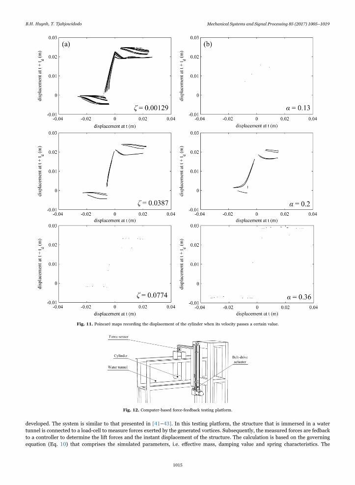
Fig. 11 shows the Poincaré map, which illustrates the intersection of an orbit in the phase space of the dynamical system with acertain lower-dimensional subspace. The observations from the plot also suggest the same tendency as shown in the contour plot andthe bifurcation diagrams. The maps are generated by simulating the system in a much longer period of 200,000 s after exclusion ofthe transient response, in order to have sufficient intersection points in the phase space..
The left panels of the figure, Fig. 11(a), illustrate the evolution of the Poincaré map of the system response for increasingdamping values. From the figures, it can be seen that the system results in a chaotic response when ζ=0.00129 as the Poincaré mapexhibits a fractal structure. In line with the contour map in Fig. 9, a higher damping value will suppress the chaotic behavior as themap for ζ=0.0774 comprises only a finite number of points, instead of a fractal structure formation. On the other hand, the periodicvibration turns to be chaotic when the bistable gap increases and turns to be periodic again when the bistable gap exceeds a certainvalue (see the right panels (b)).
In practice, high damping value to suppress chaotic behavior on the VIV energy generator can be attained from the damping ofthe PTO box, while designing the converter with either a small or very large bistable gap can also be useful in avoiding chaoticvibrations. However, the bistable system with a very large bistable gap tends to vibrate in the intra-well mode dominantly; thus thetechnical merit of enhancing the harvested power through the introduction of bistable spring will not be achieved.
4. Experimental validation
To verify the existence of chaotic responses on the bistable VIV system, a series of experiment is carried out on a dedicated testingplatform.
Fig. 9. Largest Lyapunov exponent of the system excited by the water flow with velocity of 0.175 m/s as a function of damping, ζ, and bistable gap, α.
B.H. Huynh, T. Tjahjowidodo Mechanical Systems and Signal Processing 85 (2017) 1005–1019
1013
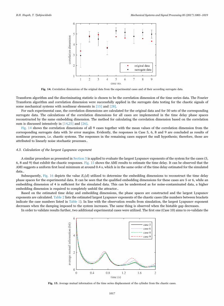
4.1. Computer-based force feedback testing platform and experimental facilities
A computer based testing platform to facilitate experiments of VIV structure with varying governing parameters is designed and
Fig. 10. Vibrating amplitude response of the system with different values of damping and bistable gap under the change of water flow velocity.
B.H. Huynh, T. Tjahjowidodo Mechanical Systems and Signal Processing 85 (2017) 1005–1019
1014
developed. The system is similar to that presented in [41–43]. In this testing platform, the structure that is immersed in a watertunnel is connected to a load-cell to measure forces exerted by the generated vortices. Subsequently, the measured forces are fedbackto a controller to determine the lift forces and the instant displacement of the structure. The calculation is based on the governingequation (Eq. 10) that comprises the simulated parameters, i.e. effective mass, damping value and spring characteristics. The
Fig. 11. Poincaré maps recording the displacement of the cylinder when its velocity passes a certain value.
B.H. Huynh, T. Tjahjowidodo Mechanical Systems and Signal Processing 85 (2017) 1005–1019
1015
calculated displacement is sent to an actuator in the testing platform to drive the VIV structure. The concept of the testing platform isshown illustratively in Fig. 12..
The main advantage of this testing platform is that the physical parameters of the system, e.g. the effective mass, damping andspring characteristics can be virtually, yet easily, imposed to the system. Particularly, the bistable restoring force function (Eq. 3) canbe easily prescribed into the system through the controller to apply various bistable springs, without having a need to physically alterit.
m y t c y t k y t F t ( ) + ( ) + ( ) = ( )virtual virtual virtual lift (10)
The water tunnel at the Maritime Research Center, Nanyang Technological University, facilitated the experiments. The facility isable to deliver water flow velocity from 0.02–0.7 m/s which is conditioned to the uniformity of within 1.5% across the testing sectionand the turbulence intensity of below 2%. The dimension of the water tunnel is 45×31×500 cm (H×W×L), while the VIV structure, ina form of cylinder, has a length of 23.5 cm and the diameter of 5 cm. A set of physical parameters ofm*=10.1 and ζ0=0.00129 and fn,water=0.7 Hz, which were also utilized in Section 3, are applied in the experiment. The time series displacement data of the cylinder isrecorded through an 8192 pulse/rev encoder installed in the servo motor, which is connected to the belt-drive actuator that drivesthe cylinder. A set of parameters as listed in Table 1 are prescribed to the system to investigate different effects of governingparameters. In order to assure the reliability of the experimental data, 3×10⁶ data points were recorded for every 0.002 s for each setof data after the response was completely in steady-state condition, resulting in almost two hours data length.
4.2. Surrogate data testing
Fig. 13 illustrates the displacement data of the cylinder in the VIV system from cases 7 and 8. At a glance, one may see a regularresponse in Case 7 and (more) irregular behavior in Case 8. Even though regular behavior is observed in Case 7; however, it isobserved slight irregularity that is potentially attributed to the random noise. Therefore, in order to avoid bias assumption indistinguishing periodic responses from chaotic ones, a surrogate data testing is performed to all sets of experimental data..
Surrogate data testing, which was studied in [44] and systematically reviewed in [45], is an effective stochastic tool that can beutilized to figure out whether the irregularity in a time series data is induced by noise (linearly stochastic process) or by the inherentnonlinearity of the system. In this method, the surrogate data is generated using a linear process that is consistent with a specifiedprocess defined in a null hypothesis. The generated surrogate data sets are defined to mimic only the linear properties of the originaldata. Subsequently, a discriminating statistic is calculated for both the original data and the surrogate data. Stochastically, if thevalue of the original data passes the hypothesis test, the irregularity on the signal is confirmed to be attributed to linear stochasticprocess, otherwise it is confirmed as a product of nonlinear processes. In this paper, the surrogate data is produced by the Fourier
Table 1Experimental cases with different parameters.
Fig. 13. Time series displacement of the cylinder from the experimental Case 7 and Case 8.
B.H. Huynh, T. Tjahjowidodo Mechanical Systems and Signal Processing 85 (2017) 1005–1019
1016
Transform algorithm and the discriminating statistic is chosen to be the correlation dimension of the time series data. The FourierTransform algorithm and correlation dimension were successfully applied in the surrogate data testing for the chaotic signals ofsome mechanical systems with nonlinear elements in [15] and [28].
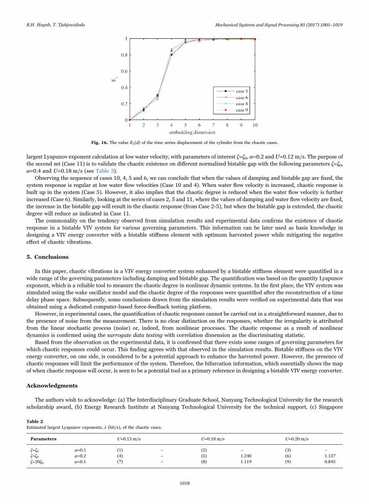
For each experimental case, the correlation dimensions are calculated for the original data and for 50 sets of the correspondingsurrogate data. The calculations of the correlation dimensions for all cases are implemented in the time delay phase spacesreconstructed by the same embedding dimension. The method for calculating the correlation dimension based on the correlationsum is discussed intensively in [14,25] and [26].
Fig. 14 shows the correlation dimensions of all 9 cases together with the mean values of the correlation dimension from thecorresponding surrogate data with 3σ error margins. Evidently, the responses in Case 5, 6, 8 and 9 are concluded as results ofnonlinear processes, i.e. chaotic systems. The responses in the remaining cases support the null hypothesis; therefore, those areattributed to linearly noise stochastic processes..
4.3. Calculation of the largest Lyapunov exponent
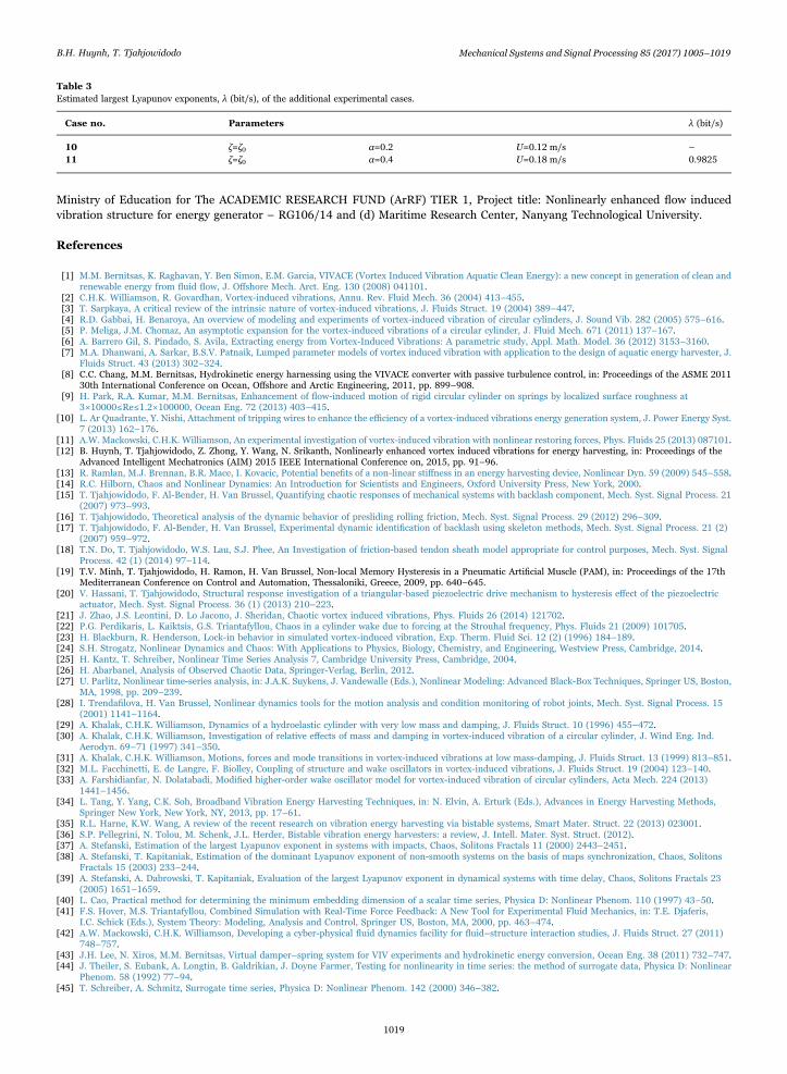
A similar procedure as presented in Section 3 is applied to evaluate the largest Lyapunov exponents of the system for the cases (5,6, 8 and 9) that exhibit the chaotic responses. Fig. 15 shows the AMI results to estimate the time delay. It can be observed that theAMI suggests a uniform first local minimum at around 0.4 s, which is in the same order of the time delay estimated for the simulateddata..
Subsequently, Fig. 16 depicts the value E1(d) utilized to determine the embedding dimensions to reconstruct the time delayphase spaces for the experimental data. It can be seen that the qualified embedding dimensions for these cases are 5 or 6, while anembedding dimension of 4 is sufficient for the simulated data. This can be understood as for noise-contaminated data, a higherembedding dimension is required to completely unfold the attractor..
Based on the estimated time delay and embedding dimensions, the phase spaces are constructed and the largest Lyapunovexponents are calculated. Table 2 lists the estimated largest Lyapunov exponents of the chaotic cases (the numbers between bracketsindicate the case numbers listed in Table 1). In line with the observation results from simulation, the largest Lyapunov exponentdecreases when the damping imposed to the system increases. The same thing is observed when the bistable gap decreases.
In order to validate results further, two additional experimental cases were utilized. The first one (Case 10) aims to re-validate the
Fig. 14. Correlation dimensions of the original data from the experimental cases and of their according surrogate data.
Fig. 15. Average mutual information of the time series displacement of the cylinder from the chaotic cases.
B.H. Huynh, T. Tjahjowidodo Mechanical Systems and Signal Processing 85 (2017) 1005–1019
1017
largest Lyapunov exponent calculation at low water velocity, with parameters of interest ζ=ζ0, α=0.2 and U=0.12 m/s. The purpose ofthe second set (Case 11) is to validate the chaotic existence on different normalized bistable gap with the following parameters ζ=ζ0,α=0.4 and U=0.18 m/s (see Table 3).
Observing the sequence of cases 10, 4, 5 and 6, we can conclude that when the values of damping and bistable gap are fixed, thesystem response is regular at low water flow velocities (Case 10 and 4). When water flow velocity is increased, chaotic response isbuilt up in the system (Case 5). However, it also implies that the chaotic degree is reduced when the water flow velocity is furtherincreased (Case 6). Similarly, looking at the series of cases 2, 5 and 11, where the values of damping and water flow velocity are fixed,the increase in the bistable gap will result in the chaotic response (from Case 2-5), but when the bistable gap is extended, the chaoticdegree will reduce as indicated in Case 11.
The commonality on the tendency observed from simulation results and experimental data confirms the existence of chaoticresponse in a bistable VIV system for various governing parameters. This information can be later used as basis knowledge indesigning a VIV energy converter with a bistable stiffness element with optimum harvested power while mitigating the negativeeffect of chaotic vibrations.
5. Conclusions
In this paper, chaotic vibrations in a VIV energy converter system enhanced by a bistable stiffness element were quantified in awide range of the governing parameters including damping and bistable gap. The quantification was based on the quantity Lyapunovexponent, which is a reliable tool to measure the chaotic degree in nonlinear dynamic systems. In the first place, the VIV system wassimulated using the wake oscillator model and the chaotic degree of the responses were quantified after the reconstruction of a timedelay phase space. Subsequently, some conclusions drawn from the simulation results were verified on experimental data that wasobtained using a dedicated computer-based force-feedback testing platform.
However, in experimental cases, the quantification of chaotic responses cannot be carried out in a straightforward manner, due tothe presence of noise from the measurement. There is no clear distinction on the responses, whether the irregularity is attributedfrom the linear stochastic process (noise) or, indeed, from nonlinear processes. The chaotic response as a result of nonlineardynamics is confirmed using the surrogate data testing with correlation dimension as the discriminating statistic.
Based from the observation on the experimental data, it is confirmed that there exists some ranges of governing parameters forwhich chaotic responses could occur. This finding agrees with that observed in the simulation results. Bistable stiffness on the VIVenergy converter, on one side, is considered to be a potential approach to enhance the harvested power. However, the presence ofchaotic responses will limit the performance of the system. Therefore, the bifurcation information, which essentially shows the mapof when chaotic response will occur, is seen to be a potential tool as a primary reference in designing a bistable VIV energy converter.
Acknowledgments
The authors wish to acknowledge: (a) The Interdisciplinary Graduate School, Nanyang Technological University for the researchscholarship award, (b) Energy Research Institute at Nanyang Technological University for the technical support, (c) Singapore
Fig. 16. The value E1(d) of the time series displacement of the cylinder from the chaotic cases.
Table 2Estimated largest Lyapunov exponents, λ (bit/s), of the chaotic cases.
B.H. Huynh, T. Tjahjowidodo Mechanical Systems and Signal Processing 85 (2017) 1005–1019
1018
Ministry of Education for The ACADEMIC RESEARCH FUND (ArRF) TIER 1, Project title: Nonlinearly enhanced flow inducedvibration structure for energy generator – RG106/14 and (d) Maritime Research Center, Nanyang Technological University.
References
[1] M.M. Bernitsas, K. Raghavan, Y. Ben Simon, E.M. Garcia, VIVACE (Vortex Induced Vibration Aquatic Clean Energy): a new concept in generation of clean andrenewable energy from fluid flow, J. Offshore Mech. Arct. Eng. 130 (2008) 041101.
[2] C.H.K. Williamson, R. Govardhan, Vortex-induced vibrations, Annu. Rev. Fluid Mech. 36 (2004) 413–455.[3] T. Sarpkaya, A critical review of the intrinsic nature of vortex-induced vibrations, J. Fluids Struct. 19 (2004) 389–447.[4] R.D. Gabbai, H. Benaroya, An overview of modeling and experiments of vortex-induced vibration of circular cylinders, J. Sound Vib. 282 (2005) 575–616.[5] P. Meliga, J.M. Chomaz, An asymptotic expansion for the vortex-induced vibrations of a circular cylinder, J. Fluid Mech. 671 (2011) 137–167.[6] A. Barrero Gil, S. Pindado, S. Avila, Extracting energy from Vortex-Induced Vibrations: A parametric study, Appl. Math. Model. 36 (2012) 3153–3160.[7] M.A. Dhanwani, A. Sarkar, B.S.V. Patnaik, Lumped parameter models of vortex induced vibration with application to the design of aquatic energy harvester, J.
Fluids Struct. 43 (2013) 302–324.[8] C.C. Chang, M.M. Bernitsas, Hydrokinetic energy harnessing using the VIVACE converter with passive turbulence control, in: Proceedings of the ASME 2011
30th International Conference on Ocean, Offshore and Arctic Engineering, 2011, pp. 899–908.[9] H. Park, R.A. Kumar, M.M. Bernitsas, Enhancement of flow-induced motion of rigid circular cylinder on springs by localized surface roughness at
3×10000≤Re≤1.2×100000, Ocean Eng. 72 (2013) 403–415.[10] L. Ar Quadrante, Y. Nishi, Attachment of tripping wires to enhance the efficiency of a vortex-induced vibrations energy generation system, J. Power Energy Syst.
7 (2013) 162–176.[11] A.W. Mackowski, C.H.K. Williamson, An experimental investigation of vortex-induced vibration with nonlinear restoring forces, Phys. Fluids 25 (2013) 087101.[12] B. Huynh, T. Tjahjowidodo, Z. Zhong, Y. Wang, N. Srikanth, Nonlinearly enhanced vortex induced vibrations for energy harvesting, in: Proceedings of the
Advanced Intelligent Mechatronics (AIM) 2015 IEEE International Conference on, 2015, pp. 91–96.[13] R. Ramlan, M.J. Brennan, B.R. Mace, I. Kovacic, Potential benefits of a non-linear stiffness in an energy harvesting device, Nonlinear Dyn. 59 (2009) 545–558.[14] R.C. Hilborn, Chaos and Nonlinear Dynamics: An Introduction for Scientists and Engineers, Oxford University Press, New York, 2000.[15] T. Tjahjowidodo, F. Al-Bender, H. Van Brussel, Quantifying chaotic responses of mechanical systems with backlash component, Mech. Syst. Signal Process. 21
(2007) 973–993.[16] T. Tjahjowidodo, Theoretical analysis of the dynamic behavior of presliding rolling friction, Mech. Syst. Signal Process. 29 (2012) 296–309.[17] T. Tjahjowidodo, F. Al-Bender, H. Van Brussel, Experimental dynamic identification of backlash using skeleton methods, Mech. Syst. Signal Process. 21 (2)
(2007) 959–972.[18] T.N. Do, T. Tjahjowidodo, W.S. Lau, S.J. Phee, An Investigation of friction-based tendon sheath model appropriate for control purposes, Mech. Syst. Signal
Process. 42 (1) (2014) 97–114.[19] T.V. Minh, T. Tjahjowidodo, H. Ramon, H. Van Brussel, Non-local Memory Hysteresis in a Pneumatic Artificial Muscle (PAM), in: Proceedings of the 17th
Mediterranean Conference on Control and Automation, Thessaloniki, Greece, 2009, pp. 640–645.[20] V. Hassani, T. Tjahjowidodo, Structural response investigation of a triangular-based piezoelectric drive mechanism to hysteresis effect of the piezoelectric
actuator, Mech. Syst. Signal Process. 36 (1) (2013) 210–223.[21] J. Zhao, J.S. Leontini, D. Lo Jacono, J. Sheridan, Chaotic vortex induced vibrations, Phys. Fluids 26 (2014) 121702.[22] P.G. Perdikaris, L. Kaiktsis, G.S. Triantafyllou, Chaos in a cylinder wake due to forcing at the Strouhal frequency, Phys. Fluids 21 (2009) 101705.[23] H. Blackburn, R. Henderson, Lock-in behavior in simulated vortex-induced vibration, Exp. Therm. Fluid Sci. 12 (2) (1996) 184–189.[24] S.H. Strogatz, Nonlinear Dynamics and Chaos: With Applications to Physics, Biology, Chemistry, and Engineering, Westview Press, Cambridge, 2014.[25] H. Kantz, T. Schreiber, Nonlinear Time Series Analysis 7, Cambridge University Press, Cambridge, 2004.[26] H. Abarbanel, Analysis of Observed Chaotic Data, Springer-Verlag, Berlin, 2012.[27] U. Parlitz, Nonlinear time-series analysis, in: J.A.K. Suykens, J. Vandewalle (Eds.), Nonlinear Modeling: Advanced Black-Box Techniques, Springer US, Boston,
MA, 1998, pp. 209–239.[28] I. Trendafilova, H. Van Brussel, Nonlinear dynamics tools for the motion analysis and condition monitoring of robot joints, Mech. Syst. Signal Process. 15
(2001) 1141–1164.[29] A. Khalak, C.H.K. Williamson, Dynamics of a hydroelastic cylinder with very low mass and damping, J. Fluids Struct. 10 (1996) 455–472.[30] A. Khalak, C.H.K. Williamson, Investigation of relative effects of mass and damping in vortex-induced vibration of a circular cylinder, J. Wind Eng. Ind.
Aerodyn. 69–71 (1997) 341–350.[31] A. Khalak, C.H.K. Williamson, Motions, forces and mode transitions in vortex-induced vibrations at low mass-damping, J. Fluids Struct. 13 (1999) 813–851.[32] M.L. Facchinetti, E. de Langre, F. Biolley, Coupling of structure and wake oscillators in vortex-induced vibrations, J. Fluids Struct. 19 (2004) 123–140.[33] A. Farshidianfar, N. Dolatabadi, Modified higher-order wake oscillator model for vortex-induced vibration of circular cylinders, Acta Mech. 224 (2013)
1441–1456.[34] L. Tang, Y. Yang, C.K. Soh, Broadband Vibration Energy Harvesting Techniques, in: N. Elvin, A. Erturk (Eds.), Advances in Energy Harvesting Methods,
Springer New York, New York, NY, 2013, pp. 17–61.[35] R.L. Harne, K.W. Wang, A review of the recent research on vibration energy harvesting via bistable systems, Smart Mater. Struct. 22 (2013) 023001.[36] S.P. Pellegrini, N. Tolou, M. Schenk, J.L. Herder, Bistable vibration energy harvesters: a review, J. Intell. Mater. Syst. Struct. (2012).[37] A. Stefanski, Estimation of the largest Lyapunov exponent in systems with impacts, Chaos, Solitons Fractals 11 (2000) 2443–2451.[38] A. Stefanski, T. Kapitaniak, Estimation of the dominant Lyapunov exponent of non-smooth systems on the basis of maps synchronization, Chaos, Solitons
Fractals 15 (2003) 233–244.[39] A. Stefanski, A. Dabrowski, T. Kapitaniak, Evaluation of the largest Lyapunov exponent in dynamical systems with time delay, Chaos, Solitons Fractals 23
(2005) 1651–1659.[40] L. Cao, Practical method for determining the minimum embedding dimension of a scalar time series, Physica D: Nonlinear Phenom. 110 (1997) 43–50.[41] F.S. Hover, M.S. Triantafyllou, Combined Simulation with Real-Time Force Feedback: A New Tool for Experimental Fluid Mechanics, in: T.E. Djaferis,
I.C. Schick (Eds.), System Theory: Modeling, Analysis and Control, Springer US, Boston, MA, 2000, pp. 463–474.[42] A.W. Mackowski, C.H.K. Williamson, Developing a cyber-physical fluid dynamics facility for fluid–structure interaction studies, J. Fluids Struct. 27 (2011)
748–757.[43] J.H. Lee, N. Xiros, M.M. Bernitsas, Virtual damper–spring system for VIV experiments and hydrokinetic energy conversion, Ocean Eng. 38 (2011) 732–747.[44] J. Theiler, S. Eubank, A. Longtin, B. Galdrikian, J. Doyne Farmer, Testing for nonlinearity in time series: the method of surrogate data, Physica D: Nonlinear
Phenom. 58 (1992) 77–94.[45] T. Schreiber, A. Schmitz, Surrogate time series, Physica D: Nonlinear Phenom. 142 (2000) 346–382.
Table 3Estimated largest Lyapunov exponents, λ (bit/s), of the additional experimental cases.
Case no. Parameters λ (bit/s)
10 ζ=ζ0 α=0.2 U=0.12 m/s –
11 ζ=ζ0 α=0.4 U=0.18 m/s 0.9825
B.H. Huynh, T. Tjahjowidodo Mechanical Systems and Signal Processing 85 (2017) 1005–1019


![[b.h. Liddell Hart] Revolution in Warfare(Book4me.org)](https://static.documents.pub/doc/80x56/55cf8cd75503462b139008e9/bh-liddell-hart-revolution-in-warfarebook4meorg.jpg)


