Emergent vegetation, covering floodplains and wetlands, has an important role in fluvial
ecosystems being able to control the fluxes of sediment, nutrients and contaminants. Proper
understanding of flow resistance processes is crucial on the development of reliable tools for
designing non-erodible channels.
The main objective of this study is the quantification of the forces, per unit bed area, acting on
the stems and the respective coefficient. Particular goals include a characterization and
quantification of the flow within vegetated areas susceptible to be simulated by dense arrays of
vertical emergent stems and a discussion of the dependence of the drag coefficient on
parameters that characterize this kind of flows.
To achieve the goals, experimental tests simulating rigid and emergent vegetation condition
with varying and constant density of stems were performed. The data acquisition consisted
mainly in 2D instantaneous velocities maps measured with a Particle Image Velocimetry
system (PIV) and the data treatment was performed with the Double-Averaging methodology
(DAM).
The flow characterization shows an important contribution of form-induced stresses, namely
longitudinal and shear stresses which are of the order of magnitude of Reynolds stresses.
Hence, in general, these stresses should not be neglected within the balance for the flow
resistance. The results show that the drag force seems uncorrelated with the density of stems but impacted by the longitudinal variation of this. For the range of investigated Rep and m, CD
seems uncorrelated with Rep. CD is larger for lower relative flow depths, revealing the influence
(,- 3d�5-67(1) the viscous (skin) drag on the stems;
./∀0(8)
2 �3&d�5-67(8) the form drag on the bed and .
∀0(8)2 ' ()*+
(,- 3d�5-67(8) the viscous drag on the bed.
DAM will be applied in this work as a mean to obtain a physically based formulation to
compute the drag force in flows within vegetation covered boundaries, susceptible of being
simulated by arrays of rigid cylinders. Since natural systems are not homogeneous, the flow
within the stem array is influenced by several space scales, determined by the number-density
of stems and its spatial modulation.
3
The present work features the study of flows with and without spatial variability of the areal
number-density of stems along the streamwise direction. The main objective is the
quantification of the forces, per unit bed area, acting on the stems and the respective drag
coefficient. Particular goals include a characterization and quantification of the flow within
dense arrays of vertical emergent stems and a discussion of the dependence of the drag
coefficient on parameters that characterize this kind of flows.
To achieve the proposed goals, two experimental tests were carried out. One of the tests
featured a periodic distribution of stem areal number-densities with minimum and maximum
values of 400 and 1600 stems/m2. On the second test the same number of stems was distributed
uniformly on the same area as the previous test, creating an array with stem areal number-
density m=980 stems/m2. The data acquisition consisted mainly in 2D instantaneous velocities
maps measured with a Particle Image Velocimetry system (PIV).
This work is organized in four main sections. After the introduction, the experimental setup is
described. Then, the results are presented and discussed and finally the paper is closed with
the main conclusions.
2. Experimental tests
The experimental work was carried out in a 12.5 m long and 40.8 cm wide recirculating tilting
flume of the Laboratory of Hydraulics and Environment of Instituto Superior Técnico. The
flume has glass side walls, enabling flow visualization and laser illumination. A general
representation of the flume is shown in Figure 1. The flume bottom was covered with a thin
horizontal layer of gravel and sand and arrays of rigid, vertical and cylindrical stems were
randomly placed along of a 3.5 m long reach simulating emergent vegetation conditions. The
diameter of the cylindrical elements is 1.1 cm. Downstream the reach covered with vegetation,
a coarse gravel weir controlled the flow, which was subcritical both downstream and upstream
of the vegetated reach.
Figure 1. Schematic view of the recirculating tilting flume (left) and picture of the flume during the experiments (right).
Two experimental tests were performed: test A and test B, with spatially varying and constant
stem areal number-density, respectively. For test A, the stems were placed in order to create a
pattern with varying stem areal number-density with wavelength of 0.5 m (Figure 2 - top).
Each wavelength comprises a 15 cm long patch with m =1600 stems/m2 (dense patch, herein,
p0-1 and p4-5); a 15 cm long patch with m=400 stems/m2 (sparse patch, herein, p2-3 and p6-7); 10
cm long transitions patches with 980 stems/m2 in average, divided into two 5 cm-long reaches
with 1200 stems/m2 and 800 stems/m2 (p1-2 and p2-3 with decreasing m and p3-4 and p7-8 with
increasing m).
4
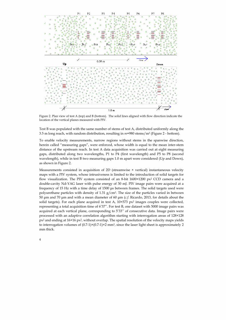
Figure 2. Plan view of test A (top) and B (bottom). The solid lines aligned with flow direction indicate the location of the vertical planes measured with PIV.
Test B was populated with the same number of stems of test A, distributed uniformly along the
3.5 m long reach, with random distribution, resulting in m=980 stems/m2 (Figure 2 - bottom).
To enable velocity measurements, narrow regions without stems in the spanwise direction,
herein called “measuring gaps”, were enforced, whose width is equal to the mean inter-stem
distance of the upstream reach. In test A data acquisition was carried out at eight measuring
gaps, distributed along two wavelengths, P1 to P4 (first wavelength) and P5 to P8 (second
wavelength), while in test B two measuring gaps 1.0 m apart were considered (Up and Down),
as shown in Figure 2.
Measurements consisted in acquisition of 2D (streamwise × vertical) instantaneous velocity
maps with a PIV system, whose intrusiveness is limited to the introduction of solid targets for
flow visualization. The PIV system consisted of an 8-bit 1600×1200 px2 CCD camera and a
double-cavity Nd-YAG laser with pulse energy of 30 mJ. PIV image pairs were acquired at a
frequency of 15 Hz with a time delay of 1500 µs between frames. The solid targets used were
polyurethane particles with density of 1.31 g/cm3. The size of the particles varied in between
50 µm and 70 µm and with a mean diameter of 60 µm (c.f. Ricardo, 2013, for details about the
solid targets). For each plane acquired in test A, 10×573 px2 images couples were collected,
representing a total acquisition time of 6’37’’. For test B, one dataset with 5000 image pairs was
acquired at each vertical plane, corresponding to 5’33’’ of consecutive data. Image pairs were
processed with an adaptive correlation algorithm starting with interrogation areas of 128×128
px2 and ending at 16×16 px2, without overlap. The spatial resolution of the velocity maps yields
to interrogation volumes of (0.7-1)×(0.7-1)×2 mm3, since the laser light sheet is approximately 2
mm thick.
5
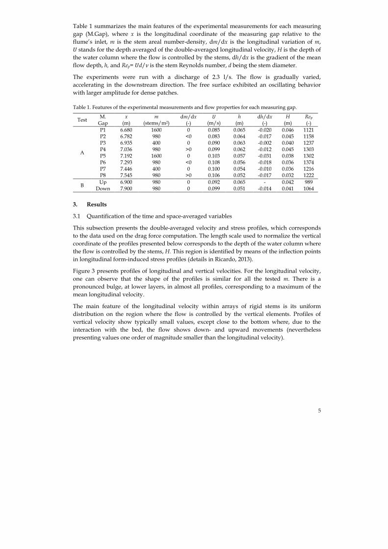
Table 1 summarizes the main features of the experimental measurements for each measuring
gap (M.Gap), where x is the longitudinal coordinate of the measuring gap relative to the
flume’s inlet, m is the stem areal number-density, dm/dx is the longitudinal variation of m,
9stands for the depth averaged of the double-averaged longitudinal velocity, H is the depth of
the water column where the flow is controlled by the stems, dh/dx is the gradient of the mean
flow depth, h, and Rep= 9d/ν is the stem Reynolds number, d being the stem diameter.
The experiments were run with a discharge of 2.3 l/s. The flow is gradually varied,
accelerating in the downstream direction. The free surface exhibited an oscillating behavior
with larger amplitude for dense patches.
Table 1. Features of the experimental measurements and flow properties for each measuring gap.
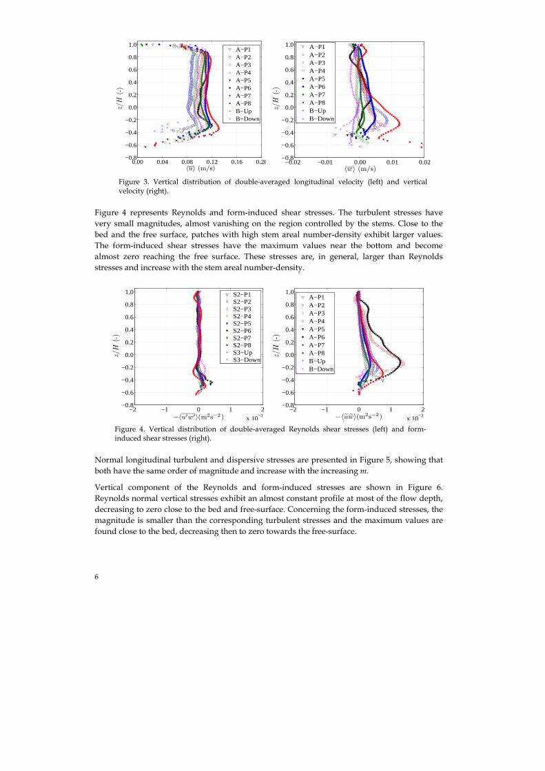
Figure 5. Vertical distribution of double-averaged Reynolds normal longitudinal stresses (left) and form-induced normal longitudinal stresses (right).
Figure 6. Vertical distribution of double-averaged Reynolds normal vertical stresses (left) and form-induced normal vertical stresses (right).
3.2 Quantification of drag forces
Integrating vertically the longitudinal component of Eq. [1], one obtains a conceptual
formulation for computing the drag force acting on the stems.
Some simplifications were considered: measurements of horizontal velocity maps showed
that⟨:⟩ ≈ 0; figures in the previous section showed that both turbulent and dispersive shear
stresses vanish at the bottom and at the free-surface; the pressure distribution was considered
hydrostatic; due to the high Reynolds number, the viscous stresses were assumed negligible;
drag forces acting on the bottom are very small compared with those acting on the stems
(Ferreira et al, 2009); it is assumed that the effect of �(�) is negligible, therefore it was
considered� = �(�), which is constant through the flow depth since the stems are vertical.
With this simplifications and incorporating the free-surface kinematic boundary condition, the
mean drag force acting on the stems per unit of plan area, ⟨=,(�)⟩, is given by (c.f. Ferreira et al
2009 for details):
0.000 0.002 0.004 0.006 0.008 0.010−0.8
−0.6
−0.4
−0.2
0.0
0.2
0.4
0.6
0.8
1.0
〈u′2
〉(m2s−2)
z/H
(-)
A−P1A−P2A−P3A−P4A−P5A−P6A−P7A−P8B−UpB−Down
0.000 0.002 0.004 0.006 0.008 0.010−0.8
−0.6
−0.4
−0.2
0.0
0.2
0.4
0.6
0.8
1.0
〈u2 〉(m2s−2)
z/H
(-)
A−P1A−P2A−P3A−P4A−P5A−P6A−P7A−P8B−UpB−Down
0.000 0.001 0.002 0.003 0.004 0.005−0.8
−0.6
−0.4
−0.2
0.0
0.2
0.4
0.6
0.8
1.0
〈w′2
〉(m2s−2)
z/H
(-)
A−P1A−P2A−P3A−P4A−P5A−P6A−P7A−P8B−UpB−Down
0.000 0.001 0.002 0.003 0.004 0.005−0.8
−0.6
−0.4
−0.2
0.0
0.2
0.4
0.6
0.8
1.0
〈w2 〉(m2s−2)
z/H
(-)
A−P1A−P2A−P3A−P4A−P5A−P6A−P7A−P8B−UpB−Down
8
⟨=�( )⟩ = "
� >−?@�⟨�⟩⟨�⟩A?� + C⟨�⟩⟨�⟩ ?�?�D − E ℎG
2?�?� − E�?ℎ
?� − ?@�⟨�I�I⟩A?� + ?ℎ
?� (�⟨�I�I⟩)|K− ?@�⟨����⟩A
?� + ?ℎ?� (�⟨����⟩)|KL
[2]
where the brackets represent integral variables as @MA = 2 Md�KN .
The mean drag force per unit of submerged stem length is defined as OP = ⟨=�( )⟩ Qℎ⁄ . The
mean drag force in the longitudinal direction is often defined in literature as the force that
balances the pressure gradient (Tanino and Nepf, 2008) by OS∗ = −� /UV
WKW,. Figure 7 shows the
values of OS and the simplification OS∗ against m. Although the pressure gradient is the
dominant term in the drag force, Figure 7 indicates that balancing the drag force only with this
term may lead to important non-systematic errors.
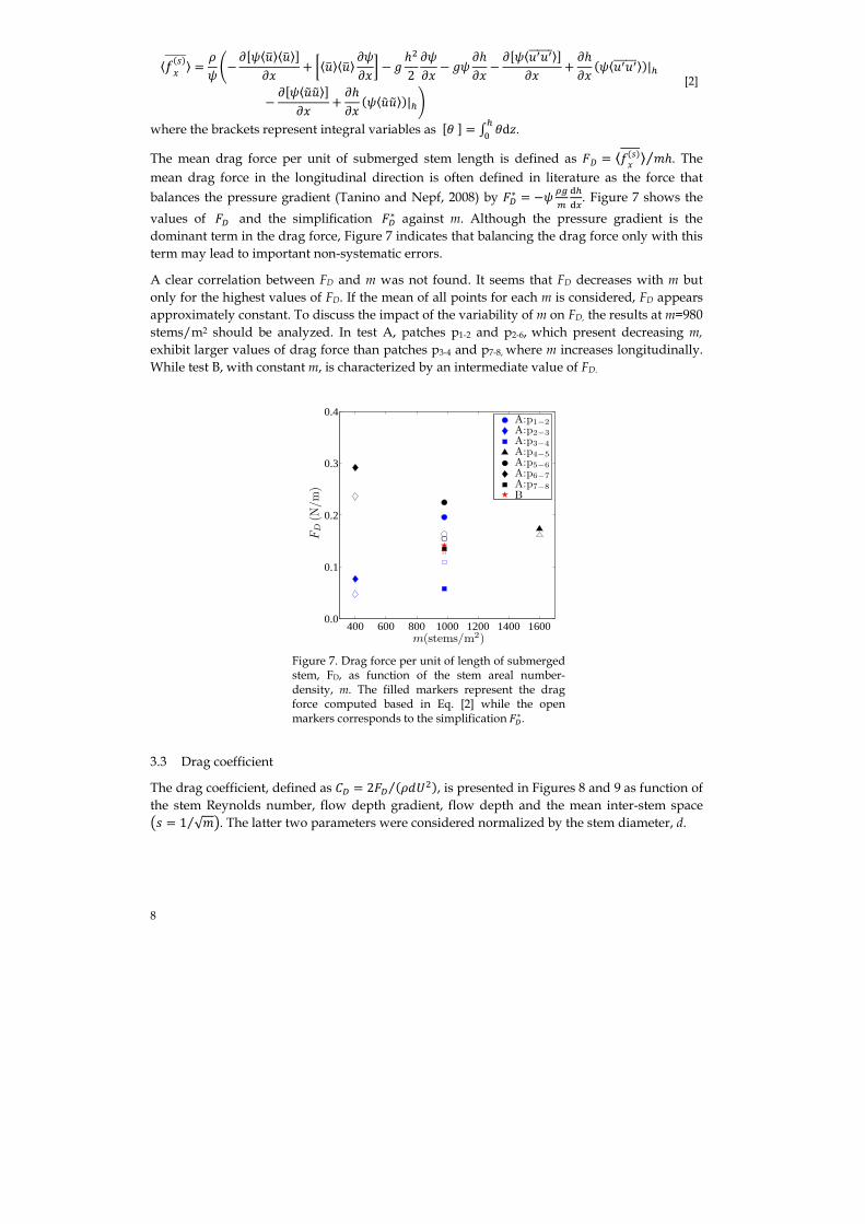
A clear correlation between FD and m was not found. It seems that FD decreases with m but
only for the highest values of FD. If the mean of all points for each m is considered, FD appears
approximately constant. To discuss the impact of the variability of m on FD, the results at m=980
stems/m2 should be analyzed. In test A, patches p1-2 and p2-6, which present decreasing m, exhibit larger values of drag force than patches p3-4 and p7-8, where m increases longitudinally.
While test B, with constant m, is characterized by an intermediate value of FD.
Figure 7. Drag force per unit of length of submerged stem, FD, as function of the stem areal number-density, m. The filled markers represent the drag force computed based in Eq. [2] while the open markers corresponds to the simplificationOS∗.
3.3 Drag coefficient
The drag coefficient, defined as XS = 2OS ("Y9G)⁄ , is presented in Figures 8 and 9 as function of
the stem Reynolds number, flow depth gradient, flow depth and the mean inter-stem space
Z = 1 √Q⁄ \. The latter two parameters were considered normalized by the stem diameter, d.
400 600 800 1000 1200 1400 16000.0
0.1
0.2
0.3
0.4
m(stems/m2)
FD
(N/m
)
A:p1−2
A:p2−3
A:p3−4
A:p4−5
A:p5−6
A:p6−7
A:p7−8
B
9
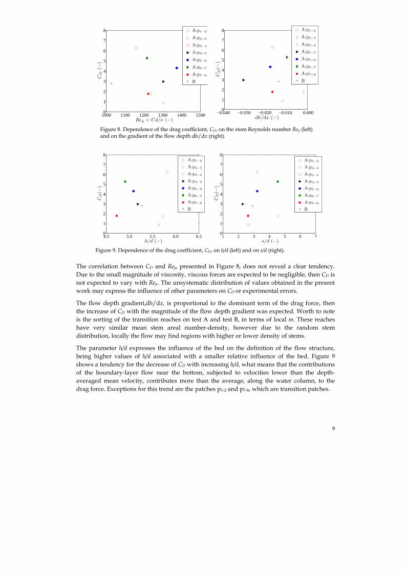
Figure 8. Dependence of the drag coefficient, CD, on the stem Reynolds number Rep (left) and on the gradient of the flow depth dh/dx (right).
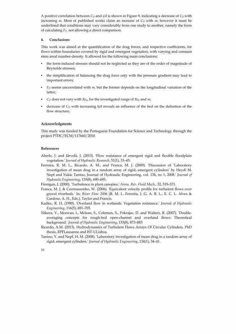
Figure 9. Dependence of the drag coefficient, CD, on h/d (left) and on s/d (right).
The correlation between CD and Rep, presented in Figure 8, does not reveal a clear tendency.
Due to the small magnitude of viscosity, viscous forces are expected to be negligible, then CD is
not expected to vary with Rep. The unsystematic distribution of values obtained in the present
work may express the influence of other parameters on CD or experimental errors.
The flow depth gradient,dh/dx, is proportional to the dominant term of the drag force, then
the increase of CD with the magnitude of the flow depth gradient was expected. Worth to note
is the sorting of the transition reaches on test A and test B, in terms of local m. These reaches
have very similar mean stem areal number-density, however due to the random stem
distribution, locally the flow may find regions with higher or lower density of stems.
The parameter h/d expresses the influence of the bed on the definition of the flow structure,
being higher values of h/d associated with a smaller relative influence of the bed. Figure 9
shows a tendency for the decrease of CD with increasing h/d, what means that the contributions
of the boundary-layer flow near the bottom, subjected to velocities lower than the depth-
averaged mean velocity, contributes more than the average, along the water column, to the
drag force. Exceptions for this trend are the patches p1-2 and p7-8, which are transition patches.
1000 1100 1200 1300 1400 15000
1
2
3
4
5
6
7
8
Rep = Ud/ν (−)
CD
(−)
A:p1−2
A:p2−3
A:p3−4
A:p4−5
A:p5−6
A:p6−7
A:p7−8
B
−0.040 −0.030 −0.020 −0.010 0.0000
1
2
3
4
5
6
7
8
dh/dx (−)
CD
(−)
A:p1−2
A:p2−3
A:p3−4
A:p4−5
A:p5−6
A:p6−7
A:p7−8
B
4.5 5.0 5.5 6.0 6.50
1
2
3
4
5
6
7
8
h/d (−)
CD
(−)
A:p1−2
A:p2−3
A:p3−4
A:p4−5
A:p5−6
A:p6−7
A:p7−8
B
1 2 3 4 5 6 70
1
2
3
4
5
6
7
8
s/d (−)
CD
(−)
A:p1−2
A:p2−3
A:p3−4
A:p4−5
A:p5−6
A:p6−7
A:p7−8
B
10
A positive correlation between CD and s/d is shown in Figure 9, indicating a decrease of CD with
increasing m. Most of published works claim an increase of CD with m; however it must be
underlined that conditions may vary considerably from one study to another, namely the form
of calculating FD, not allowing a direct comparison.
4. Conclusions
This work was aimed at the quantification of the drag forces, and respective coefficients, for
flows within boundaries covered by rigid and emergent vegetation, with varying and constant
stem areal number-density. It allowed for the following main conclusions:
• the form-induced stresses should not be neglected as they are of the order of magnitude of
Reynolds stresses;
• the simplification of balancing the drag force only with the pressure gradient may lead to
important errors;
• FD seems uncorrelated with m, but the former depends on the longitudinal variation of the
latter;
• CD does not vary with Rep, for the investigated range of Rep and m;
• decrease of CD with increasing h/d reveals an influence of the bed on the definition of the
flow structure;
Acknowledgments
This study was funded by the Portuguese Foundation for Science and Technology through the
project PTDC/ECM/117660/2010.
References
Aberle, J. and Järvelä, J. (2013). 'Flow resistance of emergent rigid and flexible floodplain
vegetation.' Journal of Hydraulic Research, 51(1), 33–45.
Ferreira, R. M. L., Ricardo, A. M., and Franca, M. J. (2009). 'Discussion of ’Laboratory
investigation of mean drag in a random array of rigid, emergent cylinders’ by Heydi M.
Nepf and Yukie Tanino, Journal of Hydraulic Engineering, vol. 134, no 1, 2008.' Journal of Hydraulic Engineering, 135(8), 690–693.
Finnigan, J. (2000). 'Turbulence in plant canopies.' Annu. Rev. Fluid Mech., 32, 519–571.
Franca, M. J. & Czernuszenko, W. (2006). 'Equivalent velocity profile for turbulent flows over
gravel riverbeds.' In: River Flow 2006 (R. M. L. Ferreira, J. G. A. B. L., E. C. L. Alves &
Cardoso, A. H., Eds.). Taylor and Francis.
Kadlec, R. H. (1990). 'Overland flow in wetlands: Vegetation resistance.' Journal of Hydraulic Engineering, 116(5), 691–705.
Nikora, V., Mcewan, I., Mclean, S., Coleman, S., Pokrajac, D. and Walters, R. (2007). 'Double-
averaging concepts for rough-bed open-channel and overland flows: Theoretical
background.' Journal of Hydraulic Engineering, 133(8), 873–883
Ricardo, A.M. (2013). Hydrodynamics of Turbulent Flows Arrays Of Circular Cylinders. PhD
thesis, EPFLausanne and IST-ULisboa.
Tanino, Y. and Nepf, H. M. (2008). 'Laboratory investigation of mean drag in a random array of
rigid, emergent cylinders.' Journal of Hydraulic Engineering, 134(1), 34–41.