Experimental Development of Compressor and Turbine ...

Experimental Development of Compressor and

Turbine Performance Maps for Turbomachinery

Aerospace Engineering Department

California Polytechnic State University, San Luis Obispo

by,

Michael W. Green

April, 2010

© 2010 Michael W. Green

California Polytechnic State University. Aerospace Engineering

April 16, 2010

1

Experimental Development of Compressor and Turbine

Performance Maps for Turbomachinery

Michael W. Green1 California Polytechnic State University, San Luis Obispo, CA, 93407

Turbomachinery performance maps are used to reveal the on and off design

performance of compressors and turbines. These maps plot the component’s pressure ratio

versus the corrected flow rate for multiple engine rotor speeds. In this experiment, a Boeing

T50-BO-8A converted turbojet engine was operated at a wide variety of rotor speeds with

orifice plates of different sizes to vary the flow rate. The corrected flow rate through the

turbojet ranged from 1.32 to 2.55 lb/s. The pressure ratios for the compressor and turbine

ranged from 2.0 to 4.3 and from 1.7 to 4.3, respectively. The resulting performance maps

showed the correct overall trend of increasing flow rate and pressure ratio with higher rotor

speeds. However, the individual speed lines were very inconsistent and lacked discernable

trends. It was concluded that bench testing the compressor and turbine components is the

ideal way to develop the performance maps.

Table of Figures ............................................................................................................................................................. 2

Nomenclature ................................................................................................................................................................ 3

I. Introduction ........................................................................................................................................................... 4

A. Compressors ..................................................................................................................................................... 4

B. Compressor Maps ............................................................................................................................................. 5

C. Turbines ............................................................................................................................................................ 6

D. Turbine Maps ................................................................................................................................................... 6

II. Apparatus .............................................................................................................................................................. 8

A. Boeing T50-BO-8A .......................................................................................................................................... 8

B. Orifice Plate Nozzle ....................................................................................................................................... 10

C. Material selection ........................................................................................................................................... 11

D. Nozzle Design ................................................................................................................................................ 11

E. Nozzle Flange Design ..................................................................................................................................... 14

F. Orifice Plate Design ....................................................................................................................................... 15

G. Nozzle Data Acquisition ................................................................................................................................. 16

III. Procedure ............................................................................................................................................................ 17

A. LabView and Remote Camera ........................................................................................................................ 17

B. Pre-Test Checks .............................................................................................................................................. 17

C. Safety Checks ................................................................................................................................................. 17

D. Turbojet Pre-Operation ................................................................................................................................... 18

E. Turbojet Operation ......................................................................................................................................... 18

F. Turbojet Shutdown ......................................................................................................................................... 18

IV. Data Analysis ...................................................................................................................................................... 19

A. Assumptions ................................................................................................................................................... 19

B. Corrected Flow Rate ....................................................................................................................................... 20

C. Pressure Ratios ............................................................................................................................................... 21

D. Efficiencies ..................................................................................................................................................... 21

E. Fuel Flow Rate ............................................................................................................................................... 21

F. Work Balance ................................................................................................................................................. 22

V. Data Validity ....................................................................................................................................................... 22

A. Turbojet Operation Envelope ......................................................................................................................... 23

1 Cal Poly Aerospace Engineering Graduate Student


April 16, 2010

2

B. Data Validity .................................................................................................................................................. 23

VI. Results and Discussion ....................................................................................................................................... 28

A. Inlet Data ........................................................................................................................................................ 28

B. Calculation of Compressor Exit Temperature ................................................................................................ 30

C. Compressor Data ............................................................................................................................................ 31

D. Combustor Data .............................................................................................................................................. 32

E. Calculation of Turbine Exit Pressure .............................................................................................................. 34

F. Turbine Data ................................................................................................................................................... 35

G. Nozzle Data .................................................................................................................................................... 36

H. Compressor Map ............................................................................................................................................ 38

I. Turbine Performance Map .............................................................................................................................. 39

VII. Conclusion .......................................................................................................................................................... 39

Table of Figures

Figure 1. Illustration of Multi-Stage Axial Compressor. ............................................................................................... 4

Figure 2. Centrifugal Compressor Wheel. ..................................................................................................................... 5

Figure 3. Typical Compressor Map. .............................................................................................................................. 5

Figure 4. Typical Turbine Map. ..................................................................................................................................... 7

Figure 5. Modified Turbine Map. .................................................................................................................................. 7

Figure 6. Gyrodyne QH-50 DASH. ............................................................................................................................... 8

Figure 7. Boeing T-50-BO-8A Cutaway. ...................................................................................................................... 9

Figure 8. Turbojet Instrumentation. ............................................................................................................................. 10

Figure 9. Conical Nozzle Design. ................................................................................................................................ 11

Figure 10. Nozzle Velocity Magnitude (in m/s) for 60% Throttle, T05 = 650°F, V5 = 300 ft/s. .................................. 12

Figure 11. Magnified View of Orifice Plate from Figure 10. ...................................................................................... 12

Figure 12. Nozzle Velocity Magnitude (in m/s) for 100% Throttle, T05 = 810°F, V5 = 500 ft/s. ................................ 13

Figure 13. Magnified View of Orifice Plate from Figure 12. ...................................................................................... 13

Figure 14. Nozzle Flanges. .......................................................................................................................................... 14

Figure 15. Boeing T-50-BO-8A with Nozzle Attached. .............................................................................................. 14

Figure 16. Finished Nozzle. ......................................................................................................................................... 15

Figure 17. Orifice Plates. ............................................................................................................................................. 15

Figure 18. Finished Orifice Plates in Descending Inside Diameter from Left to Right. .............................................. 16

Figure 19. Close-up of Chamfer Machined on Inside Edge......................................................................................... 16

Figure 20. a) Thermocouple and b) Pitot Probe in the Nozzle..................................................................................... 17

Figure 21. Theoretical Turbojet Operation Envelope. ................................................................................................. 23

Figure 22. Thrust vs. Engine Speed. ............................................................................................................................ 24

Figure 23. Compressor Exit Stagnation Temperature vs. Engine Speed. .................................................................... 24

Figure 24. Combustor Exit Stagnation Temperature vs. Engine Speed. ...................................................................... 24

Figure 25. Turbine Exit Stagnation Temperature vs. Engine Speed. ........................................................................... 25

Figure 26. Compressor Exit Temperature vs. Time. .................................................................................................... 25

Figure 27. Combustor and Turbine Exit Temperatures vs. Time. ............................................................................... 26

Figure 28. Inlet Static Pressure vs. Engine Speed. ...................................................................................................... 26

Figure 29. Inlet Stagnation Pressure vs. Engine Speed. ............................................................................................... 27

Figure 30. Compressor Exit Stagnation Pressure vs. Engine Speed. ........................................................................... 27

Figure 31. Turbine Exit Stagnation Pressure vs. Engine Speed. .................................................................................. 27

Figure 32. Corrected Flow Rate vs. Engine Speed. ..................................................................................................... 29

Figure 33. Boeing T50-BO-8A Air Flow vs. Ambient Temperature at SLS Conditions. ............................................ 29

Figure 34. Inlet Pressure Recovery vs. Engine Speed. ................................................................................................ 30

Figure 35. Illustration of Iterative Calculation of Compressor Exit Temperature. ...................................................... 31

Figure 36. Compressor Pressure Ratio vs. Engine Speed. ........................................................................................... 32

Figure 37. Compressor Efficiency vs. Engine Speed................................................................................................... 32

Figure 38. Fuel Flow Rate vs. Engine Speed. .............................................................................................................. 33

Figure 39. Fuel/Air Ratio vs. Engine Speed. ............................................................................................................... 33

Figure 40. Boeing T50-BO-8A Fuel Flow vs. Ambient Temperature at Normal Power. ............................................ 34


April 16, 2010

3

Figure 41. Turbine Pressure Ratio vs. Engine Speed. .................................................................................................. 35

Figure 42. Turbine Efficiency vs. Engine Speed. ........................................................................................................ 36

Figure 43. Nozzle Pressure Ratio vs. Engine Speed. ................................................................................................... 37

Figure 44. Nozzle Exit Mach Number vs. Engine Speed. ........................................................................................... 37

Figure 45. Compressor Performance Map. .................................................................................................................. 38

Figure 46. Turbine Performance Map. ......................................................................................................................... 39

Nomenclature

A = area, in2

Cp = specific heat at constant pressure Cv = specific heat at constant volume F = thrust, lbf H = enthalpy, BTU/lb J = conversion factor, 778 (ft-lb/BTU) M = Mach number N = Engine speed, %RPM P = pressure, lb/in2

R = universal gas constant T = temperature, °R V = velocity, ft/sec f = fuel/air ratio g = acceleration of gravity, ft/sec2

m& = mass flow rate, slugs/sec

n = engine speed, rev/min

w& = flow rate, lb/sec

δ = ambient pressure ratio η = isentropic efficiency γ = ratio of specific heats π = pressure ratio ρ = density, slugs/ft3

θ = absolute ambient temperature ratio Subscripts

a = ambient air = air only (non-combusted) comp = compressor corr = corrected exh = exhaust, air + fuel (combusted) exit = engine exit fuel = fuel i/inlet = inlet ideal = ideal/isentropic turb = turbine 0 = stagnation 2 = inlet exit/compressor inlet 3 = compressor exit/combustor inlet 4 = combustor exit/turbine inlet 5 = turbine exit 6 = nozzle inlet 7 = nozzle exit


April 16, 2010

4

I. Introduction

ERFORMANCE maps for turbomachinery, also referred to as operating maps, are an essential part of compressor and turbine design. These maps consist of simple, two-dimensional plots of pressure ratio versus

corrected flow rate. They allow the designer and operator to easily determine how the machinery will perform at nearly any on or off design condition. Performance maps also reveal the operating limits of the machinery to ensure safe operation of the device. Finally, these maps can show the efficiency of the turbine and compressor and reveal their most favorable operating points.

A. Compressors

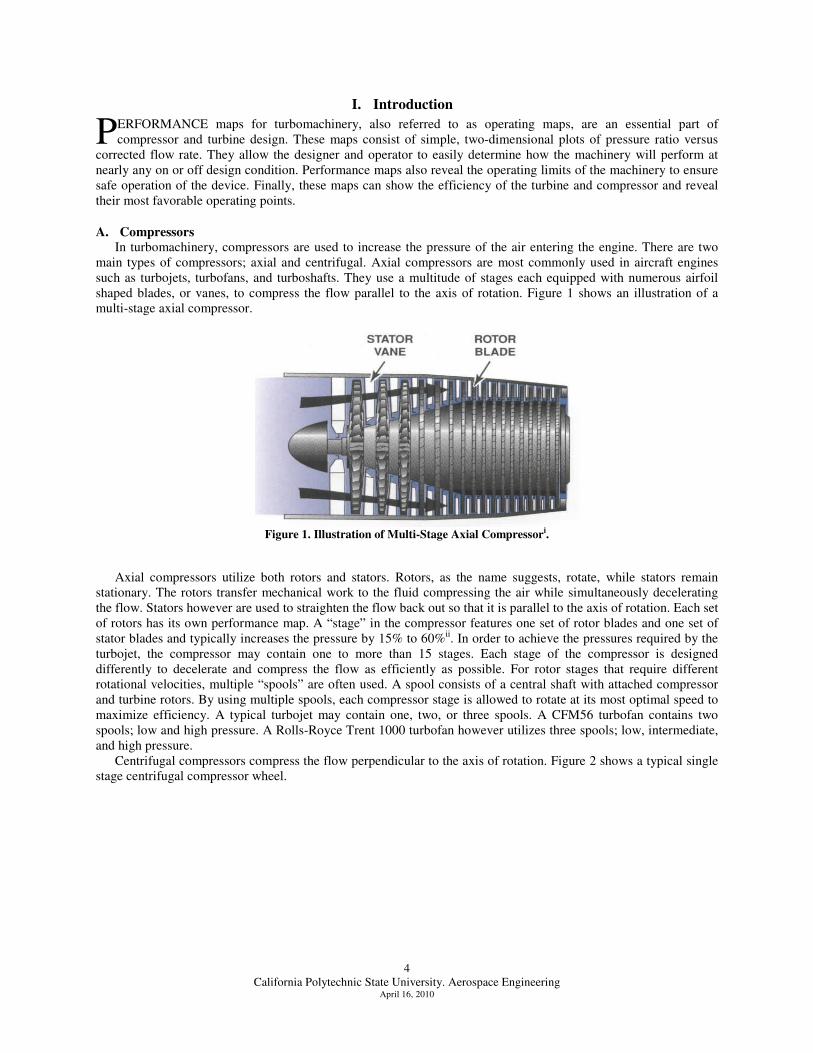
In turbomachinery, compressors are used to increase the pressure of the air entering the engine. There are two main types of compressors; axial and centrifugal. Axial compressors are most commonly used in aircraft engines such as turbojets, turbofans, and turboshafts. They use a multitude of stages each equipped with numerous airfoil shaped blades, or vanes, to compress the flow parallel to the axis of rotation. Figure 1 shows an illustration of a multi-stage axial compressor.

Figure 1. Illustration of Multi-Stage Axial Compressori.

Axial compressors utilize both rotors and stators. Rotors, as the name suggests, rotate, while stators remain stationary. The rotors transfer mechanical work to the fluid compressing the air while simultaneously decelerating the flow. Stators however are used to straighten the flow back out so that it is parallel to the axis of rotation. Each set of rotors has its own performance map. A “stage” in the compressor features one set of rotor blades and one set of stator blades and typically increases the pressure by 15% to 60%ii. In order to achieve the pressures required by the turbojet, the compressor may contain one to more than 15 stages. Each stage of the compressor is designed differently to decelerate and compress the flow as efficiently as possible. For rotor stages that require different rotational velocities, multiple “spools” are often used. A spool consists of a central shaft with attached compressor and turbine rotors. By using multiple spools, each compressor stage is allowed to rotate at its most optimal speed to maximize efficiency. A typical turbojet may contain one, two, or three spools. A CFM56 turbofan contains two spools; low and high pressure. A Rolls-Royce Trent 1000 turbofan however utilizes three spools; low, intermediate, and high pressure. Centrifugal compressors compress the flow perpendicular to the axis of rotation. Figure 2 shows a typical single stage centrifugal compressor wheel.

P


April 16, 2010

5

Figure 2. Centrifugal Compressor Wheeliii.

Unlike axial compressors, centrifugal compressors are usually only single stage and thus require only one spool. Thus, centrifugal compressors are generally easier and less expensive to manufacture. They also tend to be more reliable and compact as they contain far less moving parts. Unfortunately because centrifugal compressors are only single stage they are unable to achieve high compression ratios much above 10:1. They are most often used in small auxiliary power units (APU), air pumps, automotive turbo and superchargers, and turboshaft engines.

B. Compressor Maps

Figure 3 is an illustration of a typical compressor map from a NASA technical report on axial compressor design. The bottom axis of the plot shows the compressor corrected airflow, defined in this case as a percentage of the design corrected airflow. Oftentimes the corrected airflow will be in lbm/min or kg/s. The left axis shows the compressor pressure ratio, which is the exit pressure divided by the inlet pressure. In this case, the pressure ratio is also a defined as a percentage of the design pressure ratio.

Figure 3. Typical Compressor Mapiv.


April 16, 2010

6

The lines running up and to the left are the speed lines which represent the rotational velocity of the compressor. Again, the speed is shown as a percentage of design rotational speed, ranging from 70% to 110% (over speed). Typically, the lowest and highest speed lines represent the minimum and maximum operational speeds of the compressor, respectively. The rotational velocity can also be shown in RPM (revolutions per minute). The elliptical dashed lines represent the adiabatic efficiency “islands” of the compressor. In this case, the efficiency ranges from 70% to 88%. The dashed center line running through the middle of these islands in Figure 3 is the operating, or working line of the compressor; the line that the compressor performance follows given rotational speed and ambient conditions. Point ‘A’ shows the design point of Mach 0 at sea level at 100% throttle. Points ‘B’ and ‘C’ represent two off-design points of Mach 0.9 at altitude and Mach 2.8 at altitude, respectively. It can be seen that this compressor stage operates most efficiently at the on design condition. One final feature of a compressor map is the stall, or surge line. In Figure 3 this is shown by the solid line at the far left of the data. The surge line is determined when the compressor experiences enough back pressure to stall the airfoil shaped rotor vanes, similar to an aircraft stalling its wing at high angles of attack. If the compressor stalls it may cause a sudden backflow of air through the unit. This could lead to a flameout condition, excess component stress, and even sudden failure of the unit. It is best to avoid operating the compressor to the left of the surge line. Some compressor maps also show surge margins, which are lines to show how close the compressor is to surge. These lines can be defined many ways, but typically are a percentage of the surge air mass flow rate at a given rotational speed. For multistage compressors, each rotor stage will have its own operating map. This is because each stage is sized differently to cope with the change in pressure, temperature, and velocity of the air as it progresses through the compressor.

C. Turbines

In order to rotate the compressor, turbomachinery utilizes turbines to extract energy from the airflow. Turbines are constructed in a similar fashion to compressors with one more stages consisting of rotors and stators with airfoil shaped blades. However, turbines operate essentially the exact opposite from compressors. When the air exits the combustor, it is at a high pressure and temperature, and thus very high in energy. The turbine vanes exploit this flow and extract energy, using it to spin a central shaft that is connected to the compressor.

Turbine stages may also be located on one or more spools to optimize their speed and efficiency. Generally, turbines are more efficient than compressors, and thus less turbine stages are required to provide the mechanical energy for the compressor. Turbines are almost always axial in design as it is the most efficient design.

D. Turbine Maps

Figure 4 illustrates a typical turbine performance map using the same axes as the compressor map; pressure ratio vs. corrected airflow. In this case, the corrected airflow is in kg/s.


April 16, 2010

7

Figure 4. Typical Turbine Mapv.

Plotting the turbine performance using the same axes as the compressor map usually results in the lines getting bunched up and thus is difficult to read. Some turbine maps, instead of pressure ratio, use the change in enthalpy divided by temperature as this is a direct representation of the energy extracted. To separate the lines, the corrected airflow may be multiplied by the corrected speed. Figure 5 represents the same turbine map as Figure 4 but with the bottom axis modified to separate the lines.

Figure 5. Modified Turbine Mapv.


April 16, 2010

8

In Figure 5 the black vertical lines with slight curves at the bottom are speed lines. Each is labeled with the rotational speed as fraction of the maximum permissible speed ranging from 0.8 to 1.1 (over speed). The red dashed lines represent the isentropic efficiency hills of the turbine ranging from 75% to 85%. Finally, the yellow dots show the working line of this turbine as rotational velocity is increased. Unlike compressor maps, turbine maps do not show a surge line. This is due to the inherent design of turbines being devices that flow from high to low pressure. Due to this favorable pressure gradient, there is no back pressure on the turbine to cause stalling of the blades. Similar to the compressor, a turbine performance map will exist for each rotor stage.

II. Apparatus

A. Boeing T50-BO-8A

The experiment for this project was conducted in the Aerospace Engineering Propulsion Lab, building 41 room 144. The engine used was a Boeing T-50-BO-8A turboshaft modified to a turbojet configuration. This engine was originally produced in the early 1960’s for use on a Gyrodyne QH-50 DASH (Drone Anti-Submarine Helicopter) as shown in Figure 6.

Figure 6. Gyrodyne QH-50 DASHvi.

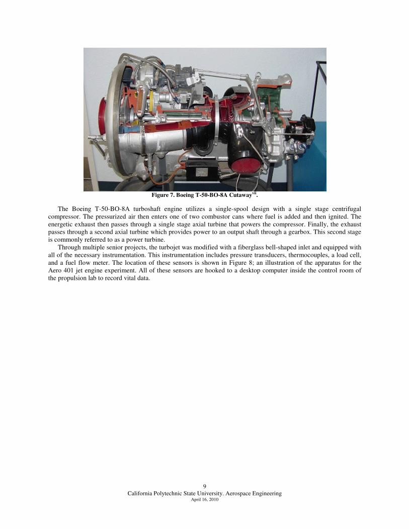
On August 12, 1960, the DASH was the first unmanned helicopter to take flight. Equipped with torpedoes, the DASH could seek out and destroy enemy submarines giving the Navy a distinct advantage. Many DASH models were equipped with the Boeing T-50-BO-8A before switching to a more powerful -12A model. The -8A model was capable of 300 Hp, giving the DASH a cruise speed of 50 knots and a range of 71 nm. A cutaway version of a Boeing T-50-BO-8A turboshaft is shown in Figure 7.


April 16, 2010

9

Figure 7. Boeing T-50-BO-8A Cutawayvii.

The Boeing T-50-BO-8A turboshaft engine utilizes a single-spool design with a single stage centrifugal compressor. The pressurized air then enters one of two combustor cans where fuel is added and then ignited. The energetic exhaust then passes through a single stage axial turbine that powers the compressor. Finally, the exhaust passes through a second axial turbine which provides power to an output shaft through a gearbox. This second stage is commonly referred to as a power turbine.

Through multiple senior projects, the turbojet was modified with a fiberglass bell-shaped inlet and equipped with all of the necessary instrumentation. This instrumentation includes pressure transducers, thermocouples, a load cell, and a fuel flow meter. The location of these sensors is shown in Figure 8; an illustration of the apparatus for the Aero 401 jet engine experiment. All of these sensors are hooked to a desktop computer inside the control room of the propulsion lab to record vital data.


April 16, 2010

10

Figure 8. Turbojet Instrumentation.

A hydraulically actuated variable area nozzle (VAN) was installed on the engine in place of the power turbine, gearbox, and output shaft. This converted the turboshaft to a turbojet and allowed the exit area of the nozzle to be varied during operation. The experiment setup for this project is essentially identical to the original Aero 401 jet engine experiment, however the VAN was replaced with a orifice plate nozzle.

B. Orifice Plate Nozzle

In order to generate the performance maps for the compressor and turbine, it was necessary to vary the airflow rate and the engine rotational speed. Varying the rotational speed is simple using the throttle lever inside the control room. To vary the airflow rate, it was necessary to restrict the flow at the nozzle end of the turbojet. The restriction must be at the nozzle end to provide backpressure to the compressor in order to find its surge line. Unfortunately, the VAN only had an exit area ranging from 39.5 in2 to 17.8 in2. From the results from the Aero 401 jet engine lab, this change in area was not enough to drastically vary the airflow rate through the turbojet.

Several methods were looked into for solving this problem. First, blockage plates were considered to further reduce the exit area of the VAN. However, these plates would require extensive machining, would heavily distort the flow field, and would require an awkward clamping system to hold the plates in place. The second option was to modify the VAN to close to a smaller area. Unfortunately this would also require extensive machining. Also, the hydraulic actuators were too long to close the nozzle far enough.

The final option was to design a new nozzle that could vary the exit area with little machining and complexity. These requirements led to a simple conical nozzle design with orifice plates of various diameters. This nozzle design is shown in Figure 9.

Bell Mouth

Inlet

Centrifugal

Compressor Combustion

Chamber Axial

Turbine

Variable Area

Nozzle

Video Camera

To PI

To P0I To P07

To P03

Thermocouple Pressure Probes

Pressure Transducers

P03 T03

T05 T04

T0I

P07

Pitot Tube

P0I

PI

Screen

Shaft

APU

Fuel Valve

Fuel Tank

Hydraulic Actuator

*Not Drawn to Scale


April 16, 2010

11

Figure 9. Conical Nozzle Design.

C. Material selection The nozzle material was chosen based on machinability, weldability, and melting temperature. The VAN that was removed from the turbojet was fabricated from stainless steel and was extremely heavy as a result. However, it was able to withstand the high exhaust gas temperatures from the turbojet. For the conical nozzle, many aluminum alloys were researched as shown in Table 1.

Table 1. List of Common Aluminum Alloys.

Aluminum

Alloy

Solidus

Temperature (°F)

Liquidus

Temperature (°F) Machinability Weldability

Price per sq. ft.

for 1/8” thick

2024-T3 935 1180 Good Low $ 27.88

5052-H32 1125 1200 Good Good $ 11.85

6061-T6 1080 1205 Good High $ 13.86

7075-T6 890 1175 Low Low $ 26.36

The temperatures and workabilities were found on MatWebviii while the prices for a square foot by 1/8 in. thick plate were found on OnlineMetalsix. The solidus temperature is when the alloy begins to melt, or begins to show properties of a liquid. The liquidus temperature occurs when the alloy becomes homogeneous and is mostly a liquid. For this reason, the solidus temperature was considered to be the maximum temperature to prevent the nozzle from warping or otherwise breaking. From the data collected during the Aero 401 jet engine lab, the maximum nozzle inlet temperature achieved was about 810°F. Alloy 5052-H32 was chosen for the conical nozzle and orifice plates due to its highest solidus temperature and its lowest price. The turbine housing flange from the VAN, made of stainless steel, was used to attach the nozzle to the turbine housing of the turbojet

D. Nozzle Design

The conical nozzle portion was made from a 0.09 in. thick sheet mainly due to the 0.10 in. limit on the sheet metal roller and cutter in the Cal Poly hanger, building 4. The nozzle was 34 in. long to prevent the recirculation zones at the orifice plate from disturbing the flow through the turbine. The nozzle inlet was 9.125 in. in diameter while the nozzle exit was 7.0 in. in diameter, resulting in a 1.7° converging half-angle. Using inlet boundary conditions derived from the Aero 401 jet engine lab, the nozzle was modeled in Gambitx and Fluentxi. The following figures show contour plots of velocity magnitude inside the nozzle during steady operation. Two different cases were then considered; steady idle at about 60% RPM and steady maximum thrust at 100% RPM. A 3.0 in. diameter orifice plates was used in these examples in order to model the most restrictive setup.

Orifice Plate

Conical Nozzle

Turbine Flange Orifice Flange

Turbine Housing Flange


April 16, 2010

12

Figure 10. Nozzle Velocity Magnitude (in m/s) for 60% Throttle, T05 = 650°F, V5 = 300 ft/s.

Figure 11. Magnified View of Orifice Plate from Figure 10.


April 16, 2010

13

Figure 12. Nozzle Velocity Magnitude (in m/s) for 100% Throttle, T05 = 810°F, V5 = 500 ft/s.

Figure 13. Magnified View of Orifice Plate from Figure 12.

Both cases were conducted using a 2nd order k-epsilon viscous model with turbulent flow. The grids for each case were also adapted to refine the mesh in necessary areas. The recirculation zone can clearly be seen in the corners were the orifice plate meets the nozzle. Here the velocity of the air is nearly zero. It can also be seen that these zones are far enough away from the turbine to mitigate flow distortion or backflow into the turbine. An interesting result from these cases is the area of very high speed flow at the leading corner of the orifice plate. For the 60% and 100% throttle cases the velocity of this flow is about 400 m/s (1312 ft/s or Mach 0.80 at T = 650°F) and 710 m/s (2329 ft/s or Mach 1.33 at T = 810°F). The supersonic flow for the 100% throttle case was of some concern, however this area was so small it was unlikely to adversely impact the results. Conversely, this supersonic flow may have acoustic implications. These Fluent cases finally show that the flow at the exit plane or the orifice plate is subsonic even at 100% throttle.


April 16, 2010

14

E. Nozzle Flange Design

The flanges for ends of the nozzle were machined from 3/16 in. thick aluminum plate due to the limited availability of thicker material. However, this thickness was felt to be sufficient as the flanges would not be under a significant amount of stress. Figure 14 shows the nozzle flanges that were machined.

Figure 14. Nozzle Flanges.

The octagonal flange on the right was designed to mate with the stainless steel turbine housing flange from the VAN. It is octagonal in shape to mitigate clearance issues with the turbojet. The circular flange was designed for the exit end of the nozzle and features four bolt holes to attach the various orifice plates. Figure 15 and Figure 16 show the turbojet with the finished nozzle attached.

Figure 15. Boeing T-50-BO-8A with Nozzle Attached.

7.0” ID 9.125” ID


April 16, 2010

15

Figure 16. Finished Nozzle.

F. Orifice Plate Design The orifice plates were machined from ¼ in. thick aluminum plate. This thickness was chosen so a 0.10 in.

chamfer could be machined on each side of the orifice for the smoothest flow possible. Before machining began however, it was realized that having chamfered edges on both sides would nearly double the machining time. Thus, the chamfer was removed from one edge and lengthened to 0.15” on the other. The chamfered edge would face the turbine during operating. Also, since these plates would also be attached to the nozzle with four bolts, a thicker material would mitigate warping and leakage. Eight differently sized orifice plates are shown in Figure 17.

Figure 17. Orifice Plates.

The inside diameters of the orifice plates range from 6.5 in. to 3.0 in. These values were chosen based on the area of the VAN which ranged from 39.5 in2 fully open to 17.8 in2 fully closed. The VAN’s fully open and closed positions corresponded to a circular diameter of 7.1 in. and 4.8 in., respectively. As mentioned previously, it was necessary to restrict the airflow rate further, so some smaller orifice diameters were chosen. An orifice diameter of 7.0 in. would be achieved by not using any orifice plate. Before machining the plates however, it was decided not to machine the 3.0 in. orifice plate. This was due to the belief that the turbojet would overheat or not even run with this much of a restriction. Furthermore, the ¼ in. plate

3.0” ID 3.5” ID 4.0” ID

5.0” ID 5.5” ID

4.5” ID

6.0” ID 6.5” ID


April 16, 2010

16

that would have been used to machine this orifice plate could be machined to a different size after initial testing to increase the fidelity of the data in interesting areas.

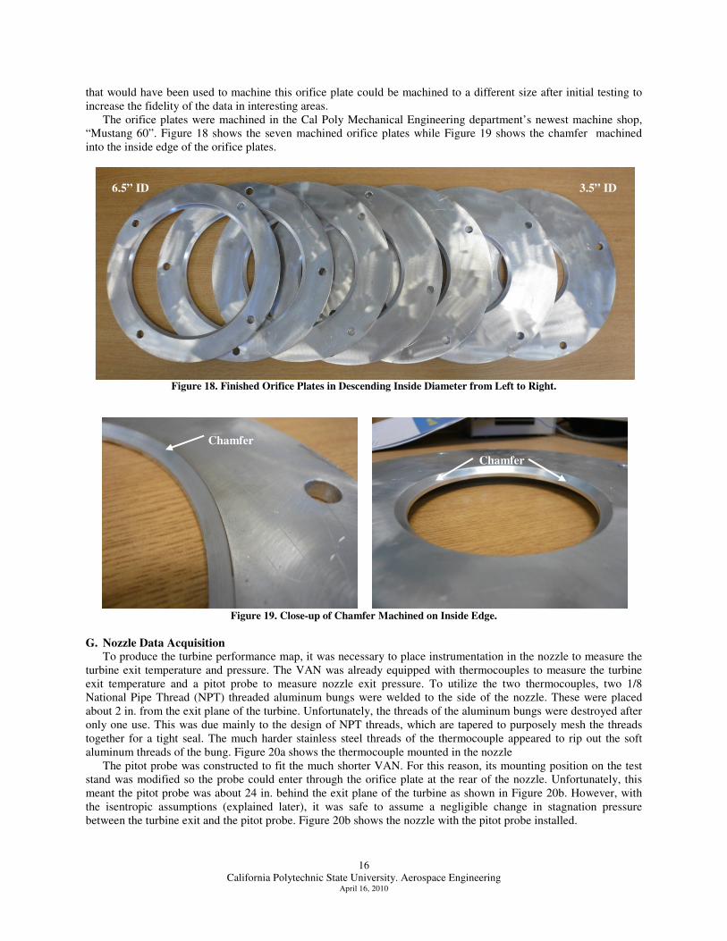
The orifice plates were machined in the Cal Poly Mechanical Engineering department’s newest machine shop, “Mustang 60”. Figure 18 shows the seven machined orifice plates while Figure 19 shows the chamfer machined into the inside edge of the orifice plates.

Figure 18. Finished Orifice Plates in Descending Inside Diameter from Left to Right.

Figure 19. Close-up of Chamfer Machined on Inside Edge.

G. Nozzle Data Acquisition

To produce the turbine performance map, it was necessary to place instrumentation in the nozzle to measure the turbine exit temperature and pressure. The VAN was already equipped with thermocouples to measure the turbine exit temperature and a pitot probe to measure nozzle exit pressure. To utilize the two thermocouples, two 1/8 National Pipe Thread (NPT) threaded aluminum bungs were welded to the side of the nozzle. These were placed about 2 in. from the exit plane of the turbine. Unfortunately, the threads of the aluminum bungs were destroyed after only one use. This was due mainly to the design of NPT threads, which are tapered to purposely mesh the threads together for a tight seal. The much harder stainless steel threads of the thermocouple appeared to rip out the soft aluminum threads of the bung. Figure 20a shows the thermocouple mounted in the nozzle

The pitot probe was constructed to fit the much shorter VAN. For this reason, its mounting position on the test stand was modified so the probe could enter through the orifice plate at the rear of the nozzle. Unfortunately, this meant the pitot probe was about 24 in. behind the exit plane of the turbine as shown in Figure 20b. However, with the isentropic assumptions (explained later), it was safe to assume a negligible change in stagnation pressure between the turbine exit and the pitot probe. Figure 20b shows the nozzle with the pitot probe installed.

6.5” ID 3.5” ID

Chamfer

Chamfer


April 16, 2010

17

Figure 20. a) Thermocouple and b) Pitot Probe in the Nozzle.

III. Procedure

The procedures of this experiment followed closely those of the jet engine lab in Aero 401. These procedures include setting up LabView to collect data, pre-test checks, safety checks, operational procedures, and post-test checks. The following sections provide detailed instructions for conducting the experiment.

A. LabView and Remote Camera

1) Turn on LabView computer(gray) located on the table in the control room. Login: aero, Password: aero 2) Turn on camera computer(white) located under the table in the control room. Login: Aero, Password: none 3) On the LabView computer open the turbojet virtual instruments (VI) file for LabView. 4) In the block diagram window, change the filename and directory to correspond with the test being

conducted. 5) Run the VI and make sure the data is reading correctly. 6) Record approximately two minutes of data to use as tare values for the calculations. 7) On the camera computer open the web cam program located on the desktop and make sure the camera is

working correctly. Do not capture video. 8) On the turbojet test stand, point camera to view area of interest. For some of the tests the camera was

pointed at the nozzle exit pitot tube. In other tests it was pointed directly at the nozzle.

B. Pre-Test Checks

1) Record ambient temperature and pressure. 2) Open both lab roll-up doors to the test cell. 3) Roll the blue acoustic absorbing blocks out of the test cell into the area behind the turbojet. Make sure they

are not placed immediately behind the turbojet nozzle. 4) Add fuel to the gas tank outside of the lab. Use Jet-A fuel only. The tank holds 13 gallons and should

contain about 1 gallon per 2 minutes of expected engine run time to ensure the turbojet does not run out of fuel.

5) Leave the gas cap loose to allow air to enter the tank during testing. 6) Open the two fuel ball valves, one located under the fuel tank and one on the turbojet test stand. 7) Plug the battery cart charger into the wall and the large red plug into the test stand. The red plug should

have a ‘+’ and a ‘-‘ facing up when plugged in. 8) Install the desired orifice plate onto nozzle with the four bolts. 9) Move the nozzle exit pitot tube into position and tighten the two bolts. It should be placed as far into the

nozzle as possible without touching the orifice plate. 10) Check the turbojet oil and add if necessary.

C. Safety Checks

1) Check to make sure no plastic tubing is touching the surfaces of the turbojet 2) Check for and remove loose or flammable debris in the test cell area. 3) Make sure the fire extinguisher is accessible and charged.

a) b)


April 16, 2010

18

4) Place a bucket under the oil drain tube. 5) Make sure all personnel are out of the test cell. 6) Check the EGT chart for the maximum allowable T05 given the ambient temperature.

D. Turbojet Pre-Operation

1) Switch all three display panels to the “ON” position. 2) Check that all temperature displays are showing degrees Fahrenheit. 3) Make sure all sensors are reading properly and are close to the values of LabView. 4) Switch on the “Engine Master” and “Oil Fan” switches. 5) Make sure the voltmeter reads at least 24V. If not, do not attempt to start turbojet. 6) Toggle the “Fuel Pump” switch to the “OFF” position. 7) Toggle the “Ignition” switch “ON” and make sure the ignition system is audible. 8) Switch the “Fuel Boost Pump” switch “ON” and make sure there is at least 35 psi of fuel pressure, and then

switch it “OFF”. 9) Toggle the “Starter” on for about 5 seconds and make sure there is oil pressure.

E. Turbojet Operation 1) Begin recording data in LabView. Set RPM to zero. 2) Operate throttle lever to the “MIN” position. 3) Toggle the “Fuel Pump” switch to the “OFF” position. 4) Toggle the “Fuel Boost Pump” switch to the “ON” position. 5) Toggle and hold the “Ignition” switch “ON”. 6) After 10 seconds, toggle and hold the “Starter” switch “ON”. 7) Once the engine RPM reaches 15%, toggle the “Fuel Pump” switch “ON”. 8) If turbojet is cold, T04 and T05 will exceed peak values during spool-up. Shut down the engine only if these

temperatures are exceeded for more than 5 seconds. 9) Once the engine RPM reaches 60%, toggle the “Fuel Boost Pump”, “Starter”, and “Ignition” switches

“OFF”. 10) Allow the turbojet to operate at idle speed for 1 minute for warm up. 11) Operate the throttle lever to desired engine RPM. 12) Monitor temperature transients in LabView. Once they become level, enter the corresponding engine RPM

in LabView and press “Enter”. 13) After about 10 seconds, set the RPM in LabView back to zero. The zero RPM data will separate the

transient from the steady-state data in the data file. 14) Operate the throttle level to the next RPM and repeat. Do not exceed a T04 of 1400°F or T05 of 1125°F (the

solidus temperature of the nozzle and orifice plates).

F. Turbojet Shutdown

1) Once all desired data has been recorded, stop recording data in LabView. 2) Operate the throttle lever to the “MIN” position. 3) Wait approximately 10 seconds and then toggle the “Fuel Pump” switch to the “OFF” position. 4) Once the engine RPM is below 10%, cycle the “Starter” switch “ON” until T04 stays below 450°F. Do not

exceed 15% RPM when cycling. 5) Toggle the “Engine Master” switch to the “OFF” position. These procedures were repeated for each orifice plate. The down-time between tests required to change the

orifice plate was minimized to reduce the amount of time needed for the turbojet to warm up. This resulted in less fuel being consumed for each test. Two individuals with heat resistant gloves could reduce the down-time to just a couple minutes which included changing the orifice plate, adding fuel, and resetting LabView.


April 16, 2010

19

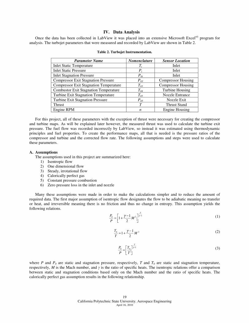
IV. Data Analysis

Once the data has been collected in LabView it was placed into an extensive Microsoft Excelxii program for analysis. The turbojet parameters that were measured and recorded by LabView are shown in Table 2.

Table 2. Turbojet Instrumentation.

Parameter Name Nomenclature Sensor Location

Inlet Static Temperature Ti Inlet

Inlet Static Pressure Pi Inlet

Inlet Stagnation Pressure P0i Inlet

Compressor Exit Stagnation Pressure P03 Compressor Housing

Compressor Exit Stagnation Temperature T03 Compressor Housing

Combustor Exit Stagnation Temperature T04 Turbine Housing

Turbine Exit Stagnation Temperature T05 Nozzle Entrance

Turbine Exit Stagnation Pressure P05 Nozzle Exit

Thrust T Thrust Stand

Engine RPM n Engine Housing

For this project, all of these parameters with the exception of thrust were necessary for creating the compressor and turbine maps. As will be explained later however, the measured thrust was used to calculate the turbine exit pressure. The fuel flow was recorded incorrectly by LabView, so instead it was estimated using thermodynamic principles and fuel properties. To create the performance maps, all that is needed is the pressure ratios of the compressor and turbine and the corrected flow rate. The following assumptions and steps were used to calculate these parameters.

A. Assumptions

The assumptions used in this project are summarized here: 1) Isentropic flow 2) One dimensional flow 3) Steady, irrotational flow 4) Calorically perfect gas 5) Constant pressure combustion 6) Zero pressure loss in the inlet and nozzle

Many these assumptions were made in order to make the calculations simpler and to reduce the amount of

required data. The first major assumption of isentropic flow designates the flow to be adiabatic meaning no transfer or heat, and irreversible meaning there is no friction and thus no change in entropy. This assumption yields the following relations.

120

2

11

−

−+=

γ

γ

γM

P

P (1)

20

2

11 M

T

T −+=

γ (2)

100

−

=

γ

γ

T

T

P

P (3)

where P and P0 are static and stagnation pressure, respectively, T and T0 are static and stagnation temperature, respectively, M is the Mach number, and γ is the ratio of specific heats. The isentropic relations offer a comparison between static and stagnation conditions based only on the Mach number and the ratio of specific heats. The calorically perfect gas assumption results in the following relationship.


April 16, 2010

20

v

p

C

C=γ (4)

where Cp is the specific heat at constant pressure and Cv is the specific heat at constant volume. The constant pressure combustion, zero pressure loss in the inlet and nozzle, and isentropic flow yield the following relations.

0403 PP = (5)

020 PP i = (6)

0705 PP = (7)

iTT 002 = (8)

where subscripts i, 2, 3, 4, 5, and 7 denote the turbojet’s inlet, compressor inlet, compressor exit, combustor exit, turbine exit, and nozzle exit stations, respectively.

B. Corrected Flow Rate

The corrected flow rate for the turbojet is the amount of air that passes through the unit per instance of time. In this project, it was defined as pounds per second (lbm/s), but is also commonly defined as slugs per second (slugs/s), pounds per hour (lb/hr), or kilograms per second (kg/s). To determine the corrected flow rate, first the correction factors were defined for temperature and pressure as shown in Equations 9 and 10, respectively.

R

Tθ a

°=

7.518 (9)

psi

Pa

689.14=δ (10)

where Ta and Pa are the ambient temperature and pressure determined before testing. These factors were necessary for referencing other parameters to standard temperature and pressure (STP) conditions. Next, the velocity in the inlet of the turbojet was calculated Bernoulli’s equation as shown in Equation 11, and the rearranged version in Equation 12.

2

02

1VPP ρ+= (11)

)(

20 iii PPV −=

ρ (12)

where P0i and Pi are the inlet stagnation and static pressure, respectively, and ρ is the density of the air entering the inlet. The inlet velocity was then entered into the mass flow rate equation represented in Equation 13 to determine the mass flow rate of air entering the turbojet.

iair AVm ρ=& (13)

where A is the cross-sectional area of the inlet. The mass flow rate was then easily converted to a flow rate using Equation 14.

airair mgw && = (14)

where g is the acceleration of gravity, assumed to be 32.174 ft/s in this project. To achieve the corrected airflow rate, the temperature and pressure corrections can be applied in Equation 15.


April 16, 2010

21

δ

θaircorrair ww && =,

(15)

This represents the amount of air entering the turbojet. In the combustor however, fuel is added to the air and thus the flow rate exiting the turbojet is slightly larger. Even though the ratio of fuel to air is very small (~0.01), it was still considered to increase accuracy. The determination of fuel flow rate is described later.

C. Pressure Ratios The pressure ratios for the both the compressor and the turbine were determined through simple calculations as

shown in Equations 16 and 17.

i

compP

P

0

03=π (16)

07

03

P

Pturb =π (17)

Both of these pressure ratios rely on the assumptions of zero pressure loss in the inlet, combustor, and nozzle. Without these assumptions, much more instrumentation would be required on the turbojet.

D. Efficiencies

The efficiencies for the compressor and turbine compare the measured enthalpy change to the ideal enthalpy change. Equations 18 and 19 represent the compressor and turbine efficiencies, respectively.

idealcomp

comp

compH

H

,∆

∆=η (18)

idealturb

turbturb

H

H

,∆

∆=η (19)

where H is enthalpy, defined in Equation 20.

TCH p= (20)

E. Fuel Flow Rate

The fuel flow rate was important for determining the amount of mass passing through the turbine. Since the fuel flow meter was not recording properly into LabView, an alternative method for determining the fuel flow rate had to be pursued. Enthalpy balance across the combustor and fuel properties were used in this case. The enthalpy balance equation written in terms of temperature is shown here in Equation 21.

03

04

03

03

04 1

T

T

TC

Q

T

T

f

p

R −

−

= (21)

where f is the fuel/air ratio and QR is the fuel heating value of the fuel, assumed to be 18,400 Btu/lbm for Jet-A. Cp, being a function of temperature and air properties, changes between the inlet and exit of the combustor. For simplification, the average combustor temperature and properties of standard air were used. Next the fuel flow rate was calculated using Equation 22 and corrected in Equation 23.

fww airfuel&& = (22)


April 16, 2010

22

θδ

fuel

corrfuel

ww

&& =,

(23)

Finally, the total flow rate exiting the turbojet through the turbine is simply the summation of the air and fuel flow rates as shown in Equation 24.

corraircorrfuelcorrexh www ,,,&&& += (24)

F. Work Balance

A fundamental property of turbomachinery is that the work done by the compressor is equal to the work done by the turbine for a steady state operating condition. This relation can be useful for determining errors in the data or calculations. The compressor and turbine work relations are shown here in Equations 25-27.

corraircompcomp wHWork ,&∆= (25)

correxhturbturb wHWork ,&∆= (26)

turbcomp WorkWork = (27)

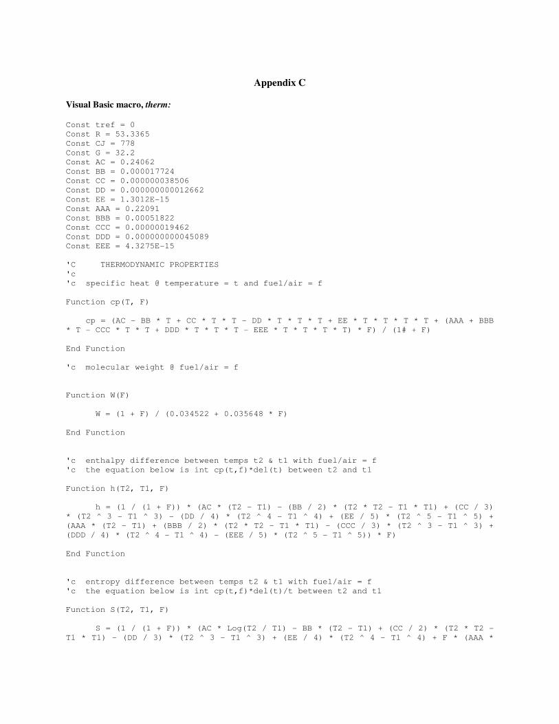
For simplification purposes, many of these equations were incorporated into an Excel Visual Basic macro named thprop, written by Mark Waters (thprop is copied into the Appendix B for reference). This macro uses simple thermodynamic relations to calculate parameters such as enthalpy, temperature, pressure, fuel/air ratio, specific heats, and more given a wide combination of inputs.

V. Data Validity

After the data was collected and averaged, it was important to analyze each measured parameter to determine the validity of the data. Small errors in the collected data can severely affect the results of the experiment. LabView recorded the turbojet data into an Excel file and included the parameters from Table 2 as well as time in seconds and engine speed in RPM. A sample raw data set is shown here in Table 3.

Table 3. Sample Raw Data Set: 7.0 in. Orifice Plate, 75% RPM.

Time

(s)

Thrust

(lbf)

T1

(°F)

T03

(°F)

T04

(°F)

T05

(°F)

Pi

(psig)

P0i

(psig)

P03

(psig)

P07

(psig)

Speed

(%)

Speed

(RPM)

96.789 22.667 74.15 270.77 932.895 687.195 0.38 0.121 22.165 0.55 75 28500

96.992 18.018 74.324 270.77 931.55 687.624 0.349 0.082 22.009 0.523 75 28500

97.195 17.992 74.107 270.974 931.277 688.587 0.414 0.105 22.229 0.606 75 28500

97.398 18.333 74.468 270.925 931.004 689.004 0.301 0.068 22.198 0.569 75 28500

97.586 19.852 74.418 270.892 929.753 689.004 0.365 0.103 22.079 0.545 75 28500

For each orifice plate diameter and engine speed, the average of the data was found and placed into a calculation spreadsheet. The average of the recorded pressure tare values was then subtracted from this data to correct the values. Table 4 shows an example of the averaged data.


April 16, 2010

23

Table 4. Sample Averaged Data: 6.0 in. Orifice Plate.

Plate Size Throttle Thrust Ti T03 T04 T05 Pi P0i P03 P07

in % RPM lbf °F °F °F °F psig psig psig psig

6.0

65% Below minimum idle

70% 29.604 63.582 240.556 940.603 718.829 -0.188 -0.021 19.548 0.974

75% 35.061 62.713 260.526 940.924 721.269 -0.212 -0.015 22.467 1.102

80% 43.295 63.461 290.627 951.843 728.256 -0.214 -0.024 26.940 1.331

85% 52.488 61.392 317.993 976.516 717.772 -0.247 -0.035 31.642 1.576

90% 63.205 60.690 350.890 1042.693 740.910 -0.291 -0.045 37.116 1.700

95% 75.917 59.987 382.372 1121.300 774.058 -0.345 -0.059 43.312 1.593

100% 86.155 61.622 411.472 1200.825 824.653 -0.382 -0.064 47.870 1.725

A. Turbojet Operation Envelope With the 6.0 in. orifice plate from the example in Table 4, the turbojet was not able to operate at 65% RPM because the minimum idle was higher than 65%. Low engine speeds were restricted by the turbojet’s minimum idle, while high engine speeds were limited by T04 or T05 temperature limits. These limits are shown in Figure 21 were derived from the experimental data. All of the test points shown in this figure were investigated in this project.

Figure 21. Theoretical Turbojet Operation Envelope.

The smaller orifice diameters reduced the minimum idle by restricting the amount of air that was allowed to pass through the turbojet. However, the smaller orifice diameters also caused to the turbojet to operate at a higher temperature. The limited temperatures occurred at the turbine inlet and the turbine exit, and both temperature limits were reached at approximately the same time. The idle and temperature limit lines cross at an orifice plate diameter of about 3.5 in. where theoretically the turbojet would idle at or above the temperature limits. These limitations severely reduced the operating range of the turbojet and the range of compressor and turbine maps.

B. Data Validity

As mentioned previously, it was necessary to determine the validity of the collected data. To do this, each measured parameter was plotted against engine speed for the various orifice plates. This would reveal any abnormalities in the data as one would expect each parameter to follow a certain trend. Figure 22 through Figure 25 show the data trends of thrust and engine temperatures.

Minimum Idle Limit

Maximum Temp Limit Theoretical Operation Envelope


April 16, 2010

24

Figure 22. Thrust vs. Engine Speed.

Figure 23. Compressor Exit Stagnation Temperature vs. Engine Speed.

Figure 24. Combustor Exit Stagnation Temperature vs. Engine Speed.

0

20

40

60

80

100

120

60% 70% 80% 90% 100%

Th

rust

(lb

f)

Engine Speed (% RPM)

7.0"

6.5"

6.0"

5.5"

5.0"

4.5"

200

250

300

350

400

450

60% 70% 80% 90% 100%

Com

pre

sso

r E

xit

Tem

per

atu

re (

F)


7.0"

6.5"

6.0"

5.5"

5.0"

4.5"

800

900

1000

1100

1200

1300

1400

60% 70% 80% 90% 100%

Com

bu

stor

Ex

it T

emp

eratu

re (

F)


7.0"

6.5"

6.0"

5.5"

5.0"

4.5"


April 16, 2010

25

Figure 25. Turbine Exit Stagnation Temperature vs. Engine Speed.

The trend of thrust vs. engine speed is very consistent and behaves as expected. Smaller orifice plates and larger engine speeds both increase the nozzle exit velocity, which directly related to gross thrust. The compressor exit temperature, T03, also behaves very well with a clear linear upward trend with higher engine speeds. However, the combustor and turbine exit temperatures, T04 and T05, seem to increase very little at low engine speeds, but then increase almost exponentially afterwards. This may be due to the fueling trends of the engine. These two temperatures also experience some unexpected dips and oscillations. The trends of these temperatures were considered in more depth by looking at the raw data. Figure 26 and Figure 27 show the variation of temperature during the experiment.

Figure 26. Compressor Exit Temperature vs. Time.

600

700

800

900

1000

1100

60% 70% 80% 90% 100%

Tu

rbin

e E

xit

Tem

per

atu

re (

F)


7.0"

6.5"

6.0"

5.5"

5.0"

4.5"

200

250

300

350

400

450

0 100 200 300 400 500 600

Com

pre

sso

r E

xit

Tem

per

atu

re (

F)

Time (s)


April 16, 2010

26

Figure 27. Combustor and Turbine Exit Temperatures vs. Time.

Each upward step in the temperatures represents an increase in engine speed. However, T03 increases very gradually while T04 and T05 increase sharply with each new engine speed. If the temperature probe is placed directly in the flow path, it is expected that the temperature would show a sharp change similar to T04 and T05. The temperature probe for T03 was placed on the very outside of the compressor casing. The ideal location is at the compressor discharge or the entrance to the combustor. For this reason it is expected that the T03 probe is underestimating the actual compressor exit temperature. This will be shown in the next section when corrections to the data are made.

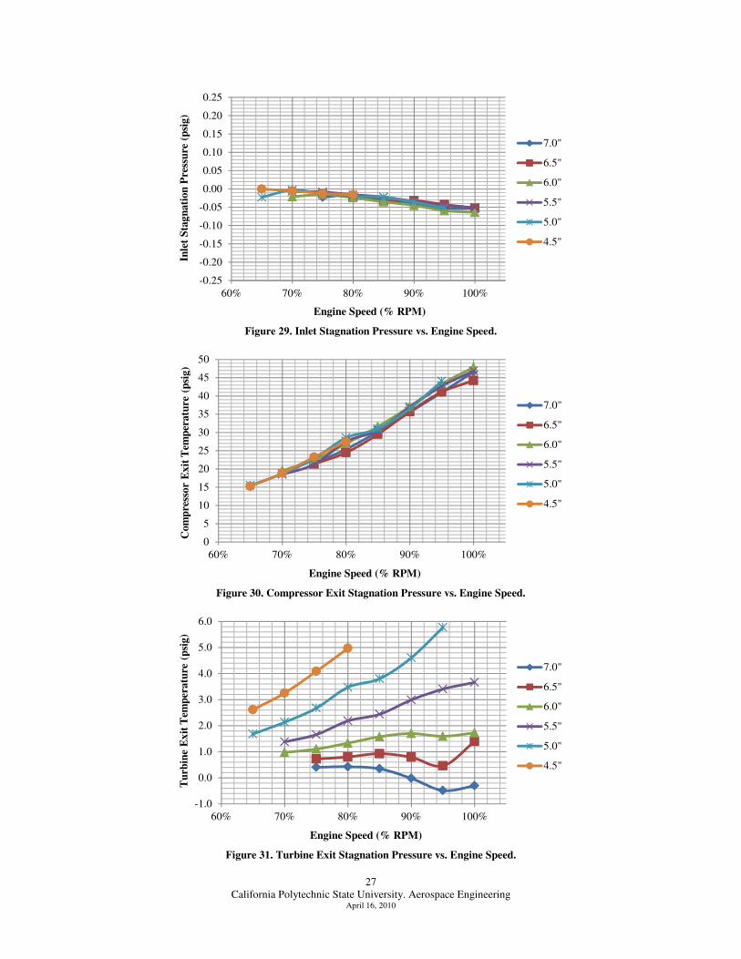
Figure 28 through Figure 31 show the trends of measured engine pressures.

Figure 28. Inlet Static Pressure vs. Engine Speed.

-0.50

-0.45

-0.40

-0.35

-0.30

-0.25

-0.20

-0.15

-0.10

-0.05

0.00

60% 70% 80% 90% 100%

Inle

t S

tati

c P

ress

ure

(p

sig

)


7.0"

6.5"

6.0"

5.5"

5.0"

4.5"


April 16, 2010

27

Figure 29. Inlet Stagnation Pressure vs. Engine Speed.

Figure 30. Compressor Exit Stagnation Pressure vs. Engine Speed.

Figure 31. Turbine Exit Stagnation Pressure vs. Engine Speed.

-0.25

-0.20

-0.15

-0.10

-0.05

0.00

0.05

0.10

0.15

0.20

0.25

60% 70% 80% 90% 100%

Inle

t S

tag

nati

on

Pre

ssu

re (

psi

g)


7.0"

6.5"

6.0"

5.5"

5.0"

4.5"

0

5

10

15

20

25

30

35

40

45

50

60% 70% 80% 90% 100%

Com

pre

sso

r E

xit

Tem

per

atu

re (

psi

g)


7.0"

6.5"

6.0"

5.5"

5.0"

4.5"

-1.0

0.0

1.0

2.0

3.0

4.0

5.0

6.0

60% 70% 80% 90% 100%

Tu

rbin

e E

xit

Tem

per

atu

re (

psi

g)


7.0"

6.5"

6.0"

5.5"

5.0"

4.5"


April 16, 2010

28

The trends of the inlet static, inlet stagnation, and compressor exit pressures, Pi, P0i, and P03, seem reasonable. As engine speed increases, static pressure through the inlet will decrease as the inlet air velocity rises. The inlet stagnation pressure should remain relatively constant but does decrease slightly due to friction losses. The turbine exit pressure, P05, does not behave as expected. While the pressure does increase with smaller orifice plates, it oscillates with engine speed for the larger orifice plates. For the 7.0 in. orifice plate, the gauge pressure drops below zero at 90% RPM. This is clearly an incorrect measurement. The reason for this is still unknown, but it likely due to unstable flow or random recirculation zones forming inside the nozzle. In the next section, the issues with compressor exit temperature, T03, and turbine exit pressure, P05, will be resolved. T03 will be calculated using a work balance method between the compressor and turbine and P05 will be calculated using the measured thrust.

VI. Results and Discussion

With the data checked, the necessary calculations could then be performed. The calculations begin at the inlet of the turbojet, step through each component, and finish at the nozzle. Sample data for each component will be shown as well as relevant figures and data trends. Once each component of the turbojet is analyzed, the resulting compressor and turbine performance maps will be shown.

A. Inlet Data

Sample calculated data for the inlet is shown in Table 5. The calculations include everything from the density of the incoming air to the corrected flow rate and Mach number.

Table 5. Sample Calculated Data for Turbojet Inlet: 7.0 in. Orifice Plate.

Test Case Inlet Data

Plate Size Throttle ρi Vi ṁ ṁcorr ẇcorr Mi T0i Pressure

in % RPM slugs/ft3 ft/s slugs/s slugs/s lb/s -- °R Recovery

7.0



75% 0.00227 114.32 0.0429 0.0439 1.41 0.101 535.46 99.84%

80% 0.00227 139.08 0.0520 0.0532 1.71 0.123 535.96 99.89%

85% 0.00226 155.48 0.0581 0.0594 1.91 0.137 535.47 99.79%

90% 0.00226 166.85 0.0622 0.0636 2.05 0.148 535.12 99.71%

95% 0.00225 167.32 0.0621 0.0636 2.05 0.148 537.17 99.64%

100% 0.00224 183.07 0.0678 0.0694 2.23 0.162 537.12 99.63%

Calculating the inlet density and velocity was necessary for determining the flow rate through the inlet, which

was used in many future calculations. For the entire experiment, the corrected flow rate ranged from 1.33 to 2.52 lb/s and is plotted in Figure 32.


April 16, 2010

29

Figure 32. Corrected Flow Rate vs. Engine Speed.

The corrected flow rate behaves as expected, increasing with engine speed. However, the flow rate also increases as the orifice plates reduce in size. This trend is the opposite of what was predicted earlier. The reason for this is still not fully understood, but is likely due to the increased nozzle pressure ratio and increased nozzle exit velocity of the smaller orifice plates. Nevertheless, the goal of the orifice plates was to vary the flow rate through the engine, and from this figure they appear to have worked. Figure 33, from the Boeing T50-BO-8A model specificationxiii, shows the engine (in its turboshaft configuration) air flow as a function of ambient temperature and power rating at sea level static conditions.

Figure 33. Boeing T50-BO-8A Air Flow vs. Ambient Temperature at SLS Conditions.

0.0

0.5

1.0

1.5

2.0

2.5

3.0

60% 70% 80% 90% 100%

Corr

ecte

d F

low

Rate

(lb

/s)


7.0"

6.5"

6.0"

5.5"

5.0"

4.5"


April 16, 2010

30

Given an ambient temperature of 74°F at normal rated power, the turbojet should consume about 4.1 lb/s of air according to the dashed red lines in Figure 33. However, the greatest air flow calculated for the turbojet was 2.52 lb/s, a 39% error. Although the turboshaft from Figure 33 is equipped with a power turbine and gearbox, it is not believed that this would cause such a significant increase in air flow. On the contrary, one would expect the air flow to decrease with the addition of a power turbine. This result aroused some suspicion about the operation of the turbojet.

The inlet Mach number was required to find T0i, the inlet stagnation temperature, and ranged from 0.09 to 0.18. The inlet pressure recovery was also calculated and is plotted in Figure 34.

Figure 34. Inlet Pressure Recovery vs. Engine Speed.

Plotting the pressure recovery of the inlet is a reliable check to see if the data is valid. From this figure, the pressure recovery ranges from 100% to about 99.6% and decreases linearly with higher engine speeds. This is expected because as engine speed is increased, the velocity through the inlet increases as well, which results in higher pressure losses due to friction. Overall, the inlet is a fairly simple component of the turbojet and was anticipated to perform as expected.

B. Calculation of Compressor Exit Temperature

Before the calculated data and relevant plots for the compressor can be presented, it was necessary to recalculate the compressor exit temperature as mentioned before. This was performed with a work balance method using the measured compressor and turbine data. Since many of the calculated parameters between the compressor, combustor, and turbine are intertwined, an iterative process was required to calculate the new compressor exit temperature. This process is illustrated in Figure 35 where calculations are performed from left to right.

99.0%

99.2%

99.4%

99.6%

99.8%

100.0%

60% 70% 80% 90% 100%

Inle

t P

ress

ure

Rec

over

y


7.0"

6.5"

6.0"

5.5"

5.0"

4.5"


April 16, 2010

31

Figure 35. Illustration of Iterative Calculation of Compressor Exit Temperature.

From this figure it can be seen that the compressor exit temperature directly affects the compressor work by altering compressor exit enthalpy, H3. However, it also affects the fuel/air ratio, f. The fuel/air ratio alters the specific heat at constant pressure, Cp, of the combustor exit and turbine exit, which alters H4 and H5. The fuel/air ratio also changes the flow rate through the turbine.

Before calculating the compressor exit temperature, the error in the work balance ranged from -2% to 57%. After a single iteration the error was reduced to about -0.15%. With the new compressor exit temperature calculated, the compressor and combustor components can now be presented.

C. Compressor Data

Unlike the inlet, the compressor of the turbojet is a much more complicated component consisting of a rotating compressor wheel and complex passageways. Some sample calculations for the turbine using the calculated compressor exit temperature are shown here in Table 6.

Table 6. Sample Calculated Data for Turbojet Compressor: 7.0 in. Orifice Plate.

Test Case Compressor Data

Plate Size Throttle πcomp T02 H2 T03 H3 ∆Hcomp ∆Hcomp,ideal Workcomp ηcomp

in % RPM -- °F Btu/lb °F Btu/lb Btu/lb Btu/lb %

7.0



75% 2.48 75.46 128.02 337.48 191.57 63.54 38.01 89.67 59.82%

80% 2.74 75.96 128.14 333.26 190.53 62.39 42.96 106.85 68.86%

85% 3.08 75.47 128.02 348.50 194.27 66.24 48.61 126.52 73.39%

90% 3.45 75.12 127.94 419.53 211.75 83.81 54.40 171.45 64.90%

95% 3.82 77.17 128.43 475.83 225.70 97.26 60.08 199.00 61.77%

100% 4.21 77.12 128.42 500.08 231.73 103.30 65.36 230.76 63.26%

The compressor calculations included many essentials such as the pressure ratio, inlet and exit enthalpies, and work done by the compressor, and the compressor isentropic efficiency. The pressure ratio ranged from 2.0 to 4.3 and is plotted in Figure 36.


April 16, 2010

32

Figure 36. Compressor Pressure Ratio vs. Engine Speed.

The trend of the compressor pressure ratio was just as expected. As the turbojet’s speed increases, the pressure ratio of the compressor increases linearly. The size of the orifice plates also appeared to have no effect on the pressure ratio. Next, the compressor efficiency is shown in Figure 37 and ranged from 37% to 80%.

Figure 37. Compressor Efficiency vs. Engine Speed.

Although less consistent than some of the other parameters, the compressor efficiency also behaved as expected. The efficiency increased with engine speed, hit a maximum, and then began to decrease. The maximum compressor efficiency occured at around 85% RPM, but does vary with orifice plate size. However, there is no discernible correlation between compressor efficiency and orifice plate size.

D. Combustor Data

Analyzing the combustor was required in order to determine the fuel flow. The fuel flow was calculated by balancing the combustor inlet and exit enthalpies using the fuel flow and fuel heating value, QR. Some sample calculations for the combustor are shown here in Table 7.

0.0

1.0

2.0

3.0

4.0

5.0

60% 70% 80% 90% 100%

Com

pre

sso

r P

ress

ure

Rati

o


7.0"

6.5"

6.0"

5.5"

5.0"

4.5"

0%

20%

40%

60%

80%

100%

60% 70% 80% 90% 100%

Com

pre

sso

r E

ffic

ien

cy (

%)


7.0"

6.5"

6.0"

5.5"

5.0"

4.5"


April 16, 2010

33

Table 7. Sample Calculated Data for Turbojet Combustor: 7.0 in. Orifice Plate.

Test Case Combustor Data

Plate Size Throttle Cp,avg f ẇfuel,corr T04 H4 ∆Hcomb

in % RPM Btu/lbm-R -- lb/s °F Btu/lb Btu/lb

7.0



75% 0.259 0.0085 0.0120 929.17 343.90 152.34

80% 0.259 0.0085 0.0146 925.76 343.00 152.47

85% 0.260 0.0086 0.0163 942.63 347.48 153.22

90% 0.262 0.0084 0.0173 1001.18 363.02 151.27

95% 0.264 0.0088 0.0180 1076.43 383.33 157.63

100% 0.265 0.0098 0.0219 1165.01 407.74 176.01

The specific heat at constant pressure was determined using the average of the inlet and exit temperatures and

was required for determining the fuel/air ratio. The fuel flow rate and fuel/air ratio in the combustor are shown in Figure 38 and Figure 39, respectively.

Figure 38. Fuel Flow Rate vs. Engine Speed.

Figure 39. Fuel/Air Ratio vs. Engine Speed.

0.000

0.005

0.010

0.015

0.020

0.025

0.030

0.035

0.040

60% 70% 80% 90% 100%

Fu

el F

low

(lb

/s)


7.0"

6.5"

6.0"

5.5"

5.0"

4.5"

0.000

0.002

0.004

0.006

0.008

0.010

0.012

0.014

60% 70% 80% 90% 100%

Fu

el/A

ir R

ati

o


7.0"

6.5"

6.0"

5.5"

5.0"

4.5"


April 16, 2010

34

The trend of fuel flow behaved as expected since it directly relates to the air flow through the combustor, which also increased with engine speed as shown in Figure 32. The fuel flow ranged from 0.012 lb/s to 0.034 lb/s. Unexpectedly, the fuel/air ratio had a clear dependency on the orifice plate size when one would expect the fuel/air ratio to remain fairly constant for most engine speeds and configurations. The smaller orifice plates also exhibit a slightly increasing fuel/air ratio with engine speed while it remains fairly constant for the larger orifice plates. The calculated fuel flow data was compared to data from Figure 40, also Boeing T50-BO-8A model specification.

Figure 40. Boeing T50-BO-8A Fuel Flow vs. Ambient Temperature at Normal Power.

Figure 40 shows the Boeing turboshaft fuel flow as a function of ambient temperature and altitude at normal rated power. Given an ambient temperature of 74°F at normal rated power, the turbojet should consume about 260 lb/hr of fuel according to the dashed red lines. For the experiment, the highest calculated fuel flow rate was 0.034 lb/s, or just 122.4 lb/hr, a 47% error. This was similar to the error in the air flow, which aroused further suspicion about the validity of the collected data. However, the fuel flow and air flow errors are similar which is expected.

E. Calculation of Turbine Exit Pressure

The turbine exit pressure, for the reasons stated earlier, needed to be calculated in order to determine the correct turbine pressure ratio. The turbine exit pressure was calculated using the measured thrust. First, the nozzle exit velocity was determined using Equation 28.

7

,V

g

wF

correxh&

= (28)

where F is thrust, ẇexh,corr is the nozzle corrected flow rate, and g is the acceleration of gravity. Using the velocity, the enthalpy drop in the nozzle was found using Equation 29.


April 16, 2010

35

gJ

VH

2

2

=∆ (29)

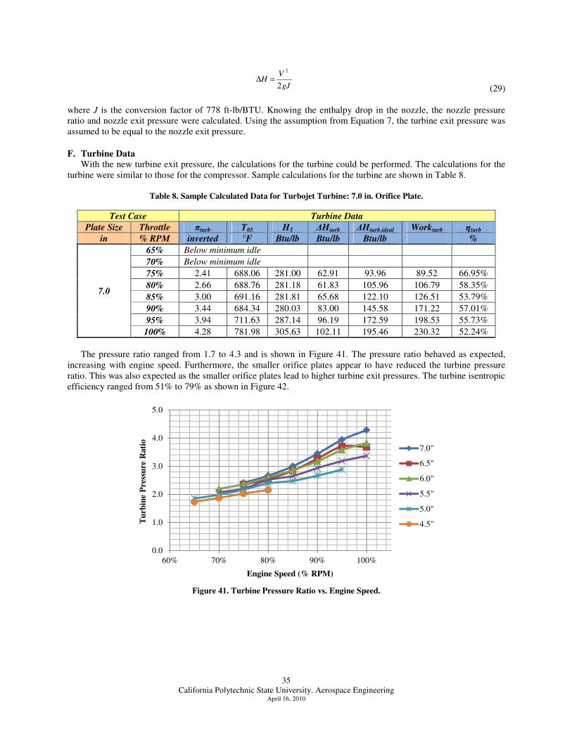
where J is the conversion factor of 778 ft-lb/BTU. Knowing the enthalpy drop in the nozzle, the nozzle pressure ratio and nozzle exit pressure were calculated. Using the assumption from Equation 7, the turbine exit pressure was assumed to be equal to the nozzle exit pressure.

F. Turbine Data

With the new turbine exit pressure, the calculations for the turbine could be performed. The calculations for the turbine were similar to those for the compressor. Sample calculations for the turbine are shown in Table 8.

Table 8. Sample Calculated Data for Turbojet Turbine: 7.0 in. Orifice Plate.

Test Case Turbine Data

Plate Size Throttle πturb T05 H5 ∆Hturb ∆Hturb,ideal Workturb ηturb

in % RPM inverted °F Btu/lb Btu/lb Btu/lb %

7.0



75% 2.41 688.06 281.00 62.91 93.96 89.52 66.95%

80% 2.66 688.76 281.18 61.83 105.96 106.79 58.35%

85% 3.00 691.16 281.81 65.68 122.10 126.51 53.79%

90% 3.44 684.34 280.03 83.00 145.58 171.22 57.01%

95% 3.94 711.63 287.14 96.19 172.59 198.53 55.73%

100% 4.28 781.98 305.63 102.11 195.46 230.32 52.24%

The pressure ratio ranged from 1.7 to 4.3 and is shown in Figure 41. The pressure ratio behaved as expected, increasing with engine speed. Furthermore, the smaller orifice plates appear to have reduced the turbine pressure ratio. This was also expected as the smaller orifice plates lead to higher turbine exit pressures. The turbine isentropic efficiency ranged from 51% to 79% as shown in Figure 42.

Figure 41. Turbine Pressure Ratio vs. Engine Speed.

0.0

1.0

2.0

3.0

4.0

5.0

60% 70% 80% 90% 100%

Tu

rbin

e P

ress

ure

Rati

o


7.0"

6.5"

6.0"

5.5"

5.0"

4.5"


April 16, 2010

36

Figure 42. Turbine Efficiency vs. Engine Speed.

The turbine efficiency appears to decrease with higher engine speeds. The efficiency also appears to have a slight dependency on the orifice plate size, where smaller orifice plates produce higher turbine efficiencies. This result seems appropriate as the turbine was likely designed to operate most efficiently with some backpressure, backpressure that could be provided by the addition of a power turbine.

G. Nozzle Data

Calculations for the nozzle were not required for this project, but were performed regardless as further checks of the data. For the nozzle, the pressure ratio, enthalpy drop, and exit Mach number were calculated as shown in Table 9. Plots of the nozzle pressure ratio and exit Mach number are shown in Figure 43 and Figure 44, respectively.

Table 9. Sample Calculated Data for Turbojet Nozzle: 7.0 in. Orifice Plate.

Test Case Nozzle Data

Plate Size Throttle πnozz V7 ∆Hnozz Mnozz

in % RPM -- ft/s Btu/lb --

7.0



75% 1.05 449.24 4.03 0.27

80% 1.05 440.68 3.88 0.27

85% 1.06 485.46 4.71 0.30

90% 1.08 530.52 5.62 0.32

95% 1.10 628.96 7.90 0.38

100% 1.12 687.73 9.45 0.40

0%

20%

40%

60%

80%

100%

60% 70% 80% 90% 100%

Com

pre

sso

r E

ffic

ien

cy (

%)


7.0"

6.5"

6.0"

5.5"

5.0"

4.5"


April 16, 2010

37

Figure 43. Nozzle Pressure Ratio vs. Engine Speed.

Figure 44. Nozzle Exit Mach Number vs. Engine Speed.

Both the nozzle pressure ratio and exit Mach number behave appropriately. Smaller orifice plates and higher engine speeds lead to greater pressures inside the nozzle, and thus higher pressure ratios. The nozzle pressure ratio ranged from 1.05 to 1.58. The Mach number was calculated to ensure that the exiting flow was subsonic for every test case, verifying the CFD simulation. The Mach number ranged from 0.27 to 0.80, concluding that the exiting flow was subsonic for every case.

0.0

0.5

1.0

1.5

2.0

60% 70% 80% 90% 100%

Nozz

le P

ress

ure

Rati

o


7.0"

6.5"

6.0"

5.5"

5.0"

4.5"

0.0

0.2

0.4

0.6

0.8

1.0

60% 70% 80% 90% 100%

Nozz

le E

xit

Mach

Nu

mb

er


7.0"

6.5"

6.0"

5.5"

5.0"

4.5"


April 16, 2010

38

H. Compressor Map

Once all of the data was analyzed and checked for errors and anomalies, the compressor map was generated. This map is shown in Figure 45.

Figure 45. Compressor Performance Map.

Unfortunately, this map bears little resemblance to a typical compressor performance map. The constant speed lines should ideally move to the right away from the stall line and then fall down as in Figure 3. These speed lines however appear to the only describe the compressor near the stall line. The speed lines move slightly to the right towards higher flow rates while maintaining a nearly constant pressure ratio. The smaller orifice plates tended to increase the flow rate, stepping the speed lines to the right. However, the final orifice plate, 4.5 in., drastically cut down the flow rate, folding the speed lines back to the left. Furthermore, the speed lines are not smooth or consistent. A clear and correct trend of this performance map is the up and to the right progression of the speed lines as the speed is increased. This is an intuitive result since higher engine speeds result in higher compressor pressure ratios and flow rates.

2.00

2.50

3.00

3.50

4.00

4.50

1.00 1.50 2.00 2.50 3.00

Com

pre

sso

r P

ress

ure

Rati

o

Corrected Flow Rate (lb/s)

65%

70%

75%

80%

85%

90%

95%

100%


April 16, 2010

39

I. Turbine Performance Map

The turbine performance map was created next and is shown in Figure 46.

Figure 46. Turbine Performance Map.

Once again, the turbine performance map minimally resembles the one shown in Figure 5. The speed lines should move to the right at low pressure ratios and then go nearly vertical as the turbine becomes choked. The low speed lines, 65%-80%, do exhibit a slight rightward trend, while the high speed lines, 85%-100%, exhibit a slight vertical trend. This may be an indication that that turbine didn’t become choked until the higher engine speeds. Similar to the compressor map, the 4.5 in. orifice plate drastically reduced the flow rate. The speed lines are also very inconsistent.

VII. Conclusion

Despite the odd nature of the resulting compressor and turbine performance maps, the experiment was an overall success. The data was collected with minimal issues and resulted in reasonable and predictable trends once the calculations were completed. The orifice plates also served their purpose of varying the flow rate through the turbojet despite them behaving the opposite of what was expected. The compressor and turbine performance maps do have a correct overall trend of increased pressure ratio and airflow with higher engine speeds. However, the individual speed lines bear little resemblance to the ideal performance maps of Figure 3 and Figure 4. The reason for this error may lay with several sources. First is that some of the data that was collected was clearly incorrect. For example, the turbine exit pressure for some of the cases dropped below zero gauge pressure. Also in some cases, the combustor exit temperature dropped as engine speed was increased. Finally, some of the recorded temperatures and pressures across the turbine resulted in incorrect isentropic efficiencies as high at 109%. While it is unlikely that these issues were caused by calculation or data acquisition errors, they may be due to the incorrect placement of vital sensors. It was shown earlier that the compressor exit temperature probe was incorrectly placed. Future investigation is needed to analyze the placement of the combustor exit and turbine exit temperature probes. The performance of the turbojet from run to run was also questionable. From this experiment and those performed in the Aero 401 laboratory, it is known that this turbojet tends to operate inconsistently despite constant procedures and testing conditions. They’re may be several reasons for this, but it is likely due to simply the antiquity of this turbojet, being produced more than four decades ago. More specifically, the fueling system is a leading culprit for the inconsistencies. Even the slightest change in fuel flow is enough to drastically affect the results. A

1.00

1.50

2.00

2.50

3.00

3.50

4.00

4.50

1.00 1.50 2.00 2.50 3.00

Tu

rbin

e P

ress

ure

Rati

o

Corrected Flow Rate (lb/s)

65%

70%

75%

80%

85%

90%

95%

100%


April 16, 2010

40

rebuild and cleaning of the fueling system including the injectors and fuel pump may alleviate some of these issues, but it is likely that these components are simply too worn and too old to work with much stability. If this experiment was to be performed again with a larger budget, the majority of time would be spent designing a variable area nozzle that does not utilize orifice plates. It is believed that the orifice plates caused some unsteady flow inside the nozzle that resulted in poor turbine exit pressure measurements. Additionally, the orifice plate nozzle required the turbojet to be shut down in order to change the orifice plate. This may have led to inconsistent tests between orifice plates as atmospheric properties do change. Even the properties (temperature, heat soak, geometry) of the turbojet could change between tests as it heats and cools, significantly affecting the results. Furthermore, some effort would be placed into rebuilding/renovating the turbojet, specifically the fueling system as mentioned previously. The ideal variable area nozzle would be able to open from a diameter larger than 7.0 in. and close down to a diameter of 4.0 in. or less. The nozzle should also be made from steel or stainless steel to be able to withstand the high turbine exit temperatures caused by high engine speeds and low nozzle exit areas. The nozzle exit area would also need to be adjustable from inside the control room. With this, the engine speed could be held constant while the exit area (and flow rate) is varied. In terms of the performance maps, this would cause the engine to move up and down a speed line instead of stepping from one speed line to the next as was done in this project. This undoubtedly would lead to smoother and more reliable speed lines. A continuously variable area nozzle would also allow for the collection of many more data points per speed line, instead of just two to six data points as the orifice plates allowed. The nozzle would also have the turbine exit pressure probe located directly behind the turbine instead of halfway down the nozzle. Essentially the ideal nozzle for this project is one similar to the original variable area nozzle but with a wider range of exit areas. Regardless, this project begged the question whether or not it is even possible to create a performance map for a compressor or turbine while they are installed into a running piece of turbomachinery. Compressors and turbines are typically “bench tested”, meaning they are installed into a very precise rig that is designed only to test that specific compressor or turbine. They are then rotated using an electric motor that is digitally controlled to maintain an exact RPM while the inlet and outlet conditions are measured using very precise instrumentation. Essentially, the compressor and turbine maps are created in the most ideal of environments. It goes without saying that the environment inside a running turbojet is far from ideal. With unsteady air entering the turbojet, various combustion instabilities, violent flow fields created by the compressor and turbine, and fluctuating rotor speeds and fuel flow rates, it may be almost impossible to generate reasonable performance maps. Furthermore, the compressor and turbine are mechanically linked by the main rotor shaft, meaning that any instability in one is transferred directly to the other. Finally, the Boeing T50-BO-8A, being an engine that is nearly half a century old, is simply not likely to operate with much reliability or consistency to begin with. Despite the issues and shortcomings of this project, an incredible amount of knowledge was gained through the analysis of the collected data. With the assistance of Mark Waters, hundreds of hours were spent scrutinizing every piece of data and every calculation. Many different approaches utilizing various thermodynamic relations were used to analyze the data. This included everything from the isentropic relations to simple enthalpy balance equations and even weight flow functions. In the end the best suited approach was chosen based on the validity of the collected data and the required calculations. Overall, this project was an incredible and unexpected learning experience. My knowledge of thermodynamics and engine cycle analysis has reached a whole new level. In terms of education and increased understanding, this project was a smashing success! Thanks To:

• Mark Waters for assistance with the data analysis

• Eric Pusle and the Mustang 60 machine shop for machining the orifice plates

• Matt Pittenger and the San Luis Jet Center for providing Jet-A fuel

• Joey Sanchez for assistance during testing i Kirk, D. R. "MAE 4261: Air-Breathing Engines." Florida Institute of Technology. 18 Nov. 2008. ii "Axial compressor." Wikipedia. 27 Apr. 2009 <http://en.wikipedia.org/wiki/Axial_compressor>. iii CC3 - Centrifugal Compressor. NASA Glenn Research Center, Cleveland, OH. iv AERODYNAMIC DESIGN OF AXIAL-FLOW COMPRESSORS. Vol. SP-36. Washington, DC: NASA, 1965. v Turbine Map. 2 Apr. 2009. GasTurb. 3 May 2009 <http://www.gasturb.de/>. vi Milestones. Gyrodyne Helicopters. 3 May 2009 <http://www.gyrodynehelicopters.com>.


April 16, 2010

41

vii Brossett, Gary, and Janet Brossett. Boeing T-50-BO-8. Pima Air and Space Museum, Tucson. viii Online Materials Information Resource. MatWeb. 04 May 2009 <http://www.matweb.com/>. ix Online Metal Store. OnlineMetals.com. 04 May 2009 <http://www.onlinemetals.com/>. x Gambit. Computer software. Vers. 2.4.6. Canonsburg, PA: ANSYS Inc., 2006. xi Fluent. Computer software. Vers. 6.3.26. Canonsburg, PA: ANSYS Inc., 2006. xii Microsoft Office Excel 2007. Vers. 2007. Microsoft, 2007. Computer software. xiii Model Specification, Engine Aircraft, Turboshaft T50-BO-8 & -8A. D4-1700-B. Boeing, 1964.

Appendix A

Test Condtions & Constants:

Di in 5.500 Plate Size De Ae

°F 74.000 Ai in2

23.758 in in in2

°R 534.000 7.0 7.0 38.485

in-Hg 29.730 6.5 6.5 33.183

psi 14.602 Type - Jet-A 6.0 6.0 28.274

θ -- 1.029 QR Btu/lbm-R 18400 5.5 5.5 23.758

δ -- 0.994 5.0 5.0 19.635

R ft-lbf/slug-°R 1716.000 4.5 4.5 15.904

γ -- 1.400 4.0 4.0 12.566

R ft-lbf/slug-°R 1544.000 3.5 3.5 9.621

γ -- 1.333

Pi P0i P03 P05

psig psig psig psig

0.477 0.103 0.593 0.150

Atmospheric Conditions

Hot

May 16, 2009, 1pm

Inlet Geometry

Pa

Orifice Plate Geometry

Ta

Cold

Fuel Data

Instrument Tares

Appendix B

Data Analysis:

Plate Size Plate Area Throttle Thrust Ti T03 T04 T05 Pi P0i P03 P05 θ Ncorr ρi Vi ṁ

in in2 % RPM lbf °F °F °F °F psig psig psig psig -- % slugs/ft

3 ft/s slugs/s

38.5 65% Below minimum idle


38.5 75% 19.870 74.369 271.533 929.166 688.064 -0.126 -0.023 21.533 0.407 1.032 73.82% 0.002274 114.321 0.043

38.5 80% 23.657 74.351 299.646 925.761 688.756 -0.168 -0.016 25.426 0.423 1.033 78.70% 0.002267 139.085 0.052

38.5 85% 29.064 73.453 330.628 942.629 691.165 -0.220 -0.030 30.239 0.347 1.032 83.66% 0.002263 155.479 0.058

38.5 90% 34.017 72.805 362.750 1001.185 684.345 -0.260 -0.042 35.586 -0.019 1.032 88.61% 0.002259 166.849 0.062

38.5 95% 40.348 74.835 390.359 1076.431 711.632 -0.271 -0.053 41.003 -0.488 1.036 93.35% 0.002249 167.319 0.062

38.5 100% 48.217 74.332 425.784 1165.007 781.976 -0.315 -0.053 46.651 -0.304 1.036 98.27% 0.002244 183.068 0.068



33.2 75% 26.800 77.647 276.157 934.669 717.439 -0.159 -0.015 21.360 0.721 1.039 73.56% 0.002255 135.739 0.050499

33.2 80% 32.072 78.427 295.666 940.065 724.874 -0.180 -0.022 24.489 0.803 1.041 78.40% 0.002248 142.266 0.052775

33.2 85% 39.787 80.226 336.098 961.919 733.983 -0.230 -0.033 29.529 0.925 1.046 83.13% 0.002233 159.248 0.058675

33.2 90% 48.324 77.511 369.005 1030.752 727.401 -0.235 -0.032 35.698 0.790 1.040 88.23% 0.002244 161.444 0.059762

33.2 95% 56.882 78.276 398.950 1091.041 750.735 -0.282 -0.043 41.122 0.460 1.043 93.03% 0.002233 175.729 0.064744

33.2 100% 62.501 74.811 414.626 1130.509 771.841 -0.312 -0.053 44.240 1.394 1.036 98.23% 0.002243 182.465 0.067520


28.3 70% 29.604 63.582 240.556 940.603 718.829 -0.188 -0.021 19.548 0.974 1.013 69.56% 0.002311 143.995 0.054900

28.3 75% 35.061 62.713 260.526 940.924 721.269 -0.212 -0.015 22.467 1.102 1.012 74.57% 0.002311 156.651 0.059724

28.3 80% 43.295 63.461 290.627 951.843 728.256 -0.214 -0.024 26.940 1.331 1.013 79.49% 0.002307 153.968 0.058609

28.3 85% 52.488 61.392 317.993 976.516 717.772 -0.247 -0.035 31.642 1.576 1.009 84.60% 0.002311 162.415 0.061928

28.3 90% 63.205 60.690 350.890 1042.693 740.910 -0.291 -0.045 37.116 1.700 1.009 89.61% 0.002307 175.289 0.066721

28.3 95% 75.917 59.987 382.372 1121.300 774.058 -0.345 -0.059 43.312 1.593 1.008 94.61% 0.002302 188.899 0.071730

28.3 100% 86.155 61.622 411.472 1200.825 824.653 -0.382 -0.064 47.870 1.725 1.012 99.40% 0.002288 200.168 0.075569


23.8 70% 35.513 78.836 252.744 999.004 787.291 -0.197 -0.007 18.498 1.379 1.043 68.55% 0.002244 156.162 0.057816

23.8 75% 41.643 79.756 274.146 1003.362 751.023 -0.206 -0.008 21.286 1.657 1.045 73.38% 0.002239 159.568 0.058939

23.8 80% 55.094 77.665 308.199 1044.621 782.492 -0.240 -0.016 27.531 2.184 1.041 78.40% 0.002242 169.754 0.062797

23.8 85% 62.795 78.999 332.436 1068.428 802.720 -0.266 -0.022 30.592 2.439 1.044 83.18% 0.002233 177.516 0.065386

23.8 90% 77.579 77.341 372.027 1142.945 849.239 -0.301 -0.034 36.992 2.989 1.041 88.19% 0.002234 185.245 0.068281

23.8 95% 91.823 77.564 399.473 1225.324 883.671 -0.346 -0.045 42.710 3.404 1.043 93.04% 0.002226 197.200 0.072428

23.8 100% 103.086 78.827 428.324 1305.508 925.737 -0.385 -0.051 46.889 3.662 1.046 97.79% 0.002215 208.341 0.076131

19.6 65% 33.929 62.269 205.451 1077.048 789.872 -0.136 -0.023 15.512 1.678 1.009 64.71% 0.002325 118.468 0.045443

19.6 70% 43.155 80.219 254.179 1099.944 862.610 -0.198 -0.003 18.676 2.133 1.046 68.46% 0.002238 158.343 0.058470

19.6 75% 53.917 77.037 278.995 1091.304 834.158 -0.227 -0.013 22.841 2.674 1.040 73.55% 0.002247 165.572 0.061378

19.6 80% 70.083 77.698 314.739 1142.891 881.658 -0.261 -0.020 28.557 3.475 1.042 78.39% 0.002239 176.161 0.065067

19.6 85% 77.562 79.017 331.787 1177.790 908.920 -0.270 -0.023 31.023 3.804 1.044 83.18% 0.002232 178.612 0.065772

19.6 90% 92.205 80.225 363.559 1255.244 972.472 -0.308 -0.036 36.563 4.606 1.047 87.95% 0.002221 188.007 0.068891

19.6 95% 115.282 80.497 402.162 1373.983 1053.824 -0.367 -0.052 44.062 5.773 1.049 92.77% 0.002211 202.452 0.073844

19.6 100% Hit T 04 limit

15.9 65% 41.252 71.877 206.812 1202.968 932.169 -0.091 0.000 15.242 2.615 1.027 64.13% 0.002290 106.895 0.040388

15.9 70% 52.029 72.260 241.089 1144.937 931.482 -0.107 -0.005 18.860 3.251 1.028 69.03% 0.002286 113.447 0.042785

15.9 75% 65.103 71.735 265.155 1197.651 975.851 -0.136 -0.012 23.274 4.086 1.028 73.98% 0.002284 125.009 0.047099

15.9 80% 79.523 72.877 291.839 1254.066 1034.045 -0.169 -0.016 27.534 4.971 1.030 78.81% 0.002273 139.372 0.052278

15.9 85% Hit T 05 limit

15.9 90% Hit T 05 limit

15.9 95% Hit T 05 limit

15.9 100% Hit T 05 limit

12.6 65% Too small to test
















Measured DataTest Case

4.5

5.0

5.5

6.5

7.0

3.5

6.0

4.0

ṁcorr ẇcorr Mi T0i Pressure πcomp ηcomp πturbine πturbine ηturbine Cp f ẇfuel,corr πnozzle ẇexh,corr H2 H3

slugs/s lb/s -- °R Recovery -- % -- inverted % Btu/lbm-R -- lb/s -- lb/s Btu/lb Btu/lb

0.044 1.411 0.101 535.458 0.998 2.479 80.85% 0.415 2.407 88.07% 0.252 0.0092 0.0129 1.028 1.424 128.023 175.452

0.053 1.713 0.123 535.963 0.999 2.744 80.11% 0.375 2.664 78.77% 0.252 0.0087 0.0150 1.029 1.728 128.144 182.310

0.059 1.910 0.137 535.466 0.998 3.077 79.48% 0.333 3.000 74.71% 0.253 0.0086 0.0164 1.024 1.926 128.025 189.888

0.064 2.046 0.148 535.123 0.997 3.447 78.91% 0.291 3.442 81.63% 0.254 0.0090 0.0184 0.999 2.064 127.942 197.767

0.064 2.046 0.148 537.167 0.996 3.822 80.06% 0.254 3.940 81.87% 0.255 0.0097 0.0199 0.967 2.066 128.434 204.558

0.069 2.234 0.162 537.124 0.996 4.210 78.24% 0.233 4.284 77.35% 0.257 0.0106 0.0236 0.979 2.257 128.423 213.298

0.052 1.667 0.119 539.18 0.9990 2.465 80.50% 0.426 2.347 81.15% 0.252 0.0092 0.0153 1.049 1.683 128.918 176.579

0.054 1.744 0.125 540.11 0.9985 2.681 81.56% 0.394 2.538 74.05% 0.252 0.0090 0.0157 1.055 1.760 129.142 181.338

0.060 1.943 0.140 542.34 0.9977 3.029 79.62% 0.352 2.842 69.79% 0.253 0.0088 0.0171 1.063 1.960 129.677 191.228

0.061 1.974 0.142 539.68 0.9978 3.452 79.23% 0.306 3.268 79.46% 0.254 0.0093 0.0184 1.054 1.992 129.038 199.304

0.067 2.141 0.155 540.85 0.9971 3.827 79.47% 0.270 3.700 78.70% 0.256 0.0098 0.0210 1.031 2.162 129.319 206.675

0.069 2.226 0.161 537.58 0.9964 4.044 78.26% 0.272 3.678 81.19% 0.257 0.0102 0.0227 1.095 2.249 128.534 210.542

0.056 1.789 0.128 525.31 0.9985 2.342 82.52% 0.456 2.192 88.92% 0.251 0.0098 0.0174 1.067 1.806 125.584 167.913

0.060 1.945 0.140 524.76 0.9990 2.541 81.85% 0.424 2.361 81.20% 0.252 0.0095 0.0185 1.075 1.964 125.452 172.771

0.059 1.910 0.137 525.43 0.9983 2.850 81.38% 0.384 2.607 74.38% 0.252 0.0092 0.0177 1.091 1.928 125.615 180.108

0.063 2.015 0.145 523.59 0.9976 3.175 80.48% 0.350 2.858 78.05% 0.253 0.0092 0.0186 1.108 2.033 125.171 186.795

0.067 2.170 0.157 523.25 0.9969 3.553 79.40% 0.315 3.172 80.16% 0.254 0.0098 0.0212 1.116 2.191 125.089 194.856

0.072 2.332 0.169 522.96 0.9959 3.982 79.26% 0.280 3.576 80.54% 0.256 0.0105 0.0245 1.109 2.357 125.020 202.592

0.077 2.462 0.179 524.96 0.9956 4.297 78.28% 0.261 3.826 79.52% 0.258 0.0113 0.0278 1.118 2.490 125.500 209.763

0.059 1.912 0.137 540.87 0.9995 2.268 82.95% 0.483 2.071 87.25% 0.252 0.0104 0.0200 1.094 1.932 129.323 170.877

0.061 1.951 0.140 541.88 0.9994 2.459 82.62% 0.453 2.207 96.09% 0.253 0.0102 0.0199 1.113 1.971 129.566 176.089

0.064 2.075 0.149 540.07 0.9989 2.889 83.81% 0.398 2.510 84.82% 0.254 0.0104 0.0215 1.150 2.096 129.130 184.400

0.067 2.164 0.156 541.62 0.9985 3.100 82.40% 0.377 2.652 80.40% 0.254 0.0104 0.0225 1.167 2.186 129.505 190.331

0.070 2.256 0.163 540.20 0.9976 3.542 80.56% 0.341 2.933 77.74% 0.256 0.0110 0.0248 1.205 2.281 129.162 200.047

0.074 2.395 0.174 540.80 0.9969 3.937 81.34% 0.314 3.183 80.71% 0.258 0.0118 0.0284 1.233 2.423 129.308 206.804

0.078 2.521 0.183 542.44 0.9965 4.226 79.90% 0.297 3.367 82.23% 0.259 0.0127 0.0320 1.251 2.553 129.702 213.926

0.046 1.478 0.106 523.44 0.9984 2.066 84.88% 0.541 1.850 131.19% 0.253 0.0122 0.0181 1.115 1.496 125.135 159.392

0.060 1.936 0.139 542.31 0.9998 2.280 83.75% 0.503 1.988 96.43% 0.254 0.0119 0.0231 1.146 1.959 129.669 171.226

0.063 2.027 0.146 539.32 0.9991 2.567 83.48% 0.461 2.167 94.34% 0.254 0.0115 0.0232 1.183 2.050 128.951 177.271

0.067 2.150 0.155 540.28 0.9986 2.960 83.76% 0.419 2.388 83.41% 0.255 0.0118 0.0253 1.238 2.176 129.183 185.999

0.068 2.176 0.157 541.67 0.9985 3.129 83.46% 0.403 2.479 80.91% 0.256 0.0120 0.0262 1.261 2.203 129.517 190.172

0.071 2.283 0.165 543.17 0.9975 3.513 83.66% 0.375 2.664 75.94% 0.258 0.0128 0.0292 1.315 2.312 129.876 197.966

0.076 2.449 0.178 543.91 0.9964 4.032 83.64% 0.347 2.879 75.19% 0.260 0.0141 0.0345 1.395 2.483 130.055 207.467

0.041 1.326 0.095 532.83 1.0000 2.044 90.11% 0.577 1.733 126.84% 0.255 0.0141 0.0187 1.179 1.344 127.391 159.722

0.044 1.405 0.100 533.33 0.9996 2.292 85.04% 0.534 1.874 91.57% 0.254 0.0128 0.0179 1.223 1.423 127.512 168.043

0.048 1.546 0.111 533.04 0.9992 2.596 86.94% 0.493 2.027 82.70% 0.255 0.0132 0.0205 1.280 1.567 127.441 173.898

0.053 1.718 0.123 534.50 0.9989 2.889 87.07% 0.465 2.153 73.64% 0.257 0.0137 0.0236 1.340 1.742 127.791 180.404

Fuel Flow Data Nozzle Data Enthalpy'sCompressor DataInlet Data Turbine Data

H4 H5 Workcomp Workturb Workerror H3,new T3,new T3,new Cp,new fnew ẇexh,corr,new H4,new H5,new Workcomp Workturb Workerror V7,calc

Btu/lb Btu/lb % Btu/lb R F Btu/lbm-R -- lb/s Btu/lb Btu/lb % ft/s

344.118 281.151 66.925 89.665 25.36% 191.57 797.48 337.48 0.259 0.0085 1.423 343.903 280.997 89.665 89.519 -0.16% 449.24

343.079 281.230 92.766 106.849 13.18% 190.53 793.26 333.26 0.259 0.0085 1.727 343.004 281.177 106.849 106.789 -0.06% 440.68

347.491 281.810 118.152 126.516 6.61% 194.27 808.50 348.50 0.260 0.0086 1.926 347.485 281.806 126.516 126.511 0.00% 485.46

363.217 280.154 142.842 171.452 16.69% 211.75 879.53 419.53 0.262 0.0084 2.063 363.023 280.027 171.452 171.220 -0.14% 530.52

383.688 287.362 155.747 198.997 21.73% 225.70 935.83 475.83 0.264 0.0088 2.064 383.329 287.138 198.997 198.534 -0.23% 628.96

408.061 305.837 189.595 230.764 17.84% 231.73 960.08 500.08 0.265 0.0098 2.256 407.740 305.635 230.764 230.322 -0.19% 687.73

345.583 288.732 79.460 95.653 16.93% 186.29 775.93 315.93 0.259 0.0089 1.682 345.484 288.658 95.653 95.582 -0.07% 512.48

346.954 290.608 91.022 99.141 8.19% 185.99 774.72 314.72 0.259 0.0090 1.759 346.946 290.603 99.141 99.136 -0.01% 586.46

352.681 292.908 119.581 117.143 -2.08% 189.97 790.98 330.98 0.260 0.0091 1.960 352.784 292.984 117.143 117.233 0.08% 653.18

371.257 291.345 138.699 159.211 12.88% 209.70 871.20 411.20 0.262 0.0090 1.992 371.134 291.263 159.211 159.079 -0.08% 780.37

387.672 297.514 165.602 194.905 15.03% 220.36 914.33 454.33 0.263 0.0093 2.161 387.473 297.385 194.905 194.657 -0.13% 846.56

398.516 303.099 182.534 214.550 14.92% 224.93 932.72 472.72 0.264 0.0097 2.247 398.297 302.958 214.550 214.259 -0.14% 894.32

347.342 289.228 75.726 104.980 27.87% 184.27 767.65 307.65 0.259 0.0091 1.805 347.124 289.067 104.980 104.809 -0.16% 527.26

347.340 289.795 92.045 113.000 18.54% 183.54 764.69 304.69 0.259 0.0091 1.963 347.224 289.708 113.000 112.901 -0.09% 574.47

350.159 291.542 104.088 113.000 7.89% 184.77 769.73 309.73 0.259 0.0092 1.928 350.154 291.538 113.000 112.996 0.00% 722.59

356.721 288.829 124.155 138.045 10.06% 193.69 806.14 346.14 0.260 0.0091 2.033 356.672 288.795 138.045 137.997 -0.03% 830.54

374.618 294.949 151.388 174.564 13.28% 205.54 854.33 394.33 0.262 0.0094 2.190 374.492 294.864 174.564 174.416 -0.08% 928.08

396.138 303.756 180.914 217.718 16.90% 218.37 906.30 446.30 0.264 0.0099 2.355 395.892 303.595 217.718 217.385 -0.15% 1036.42

418.177 317.206 207.433 251.376 17.48% 227.61 943.54 483.54 0.265 0.0106 2.488 417.868 317.006 251.376 250.927 -0.18% 1113.42

363.145 307.189 79.440 108.089 26.51% 185.86 774.18 314.18 0.260 0.0099 1.931 362.946 307.038 108.089 107.937 -0.14% 591.50

364.233 297.688 90.752 131.135 30.80% 196.79 818.77 358.77 0.261 0.0093 1.969 363.916 297.460 131.135 130.844 -0.22% 679.90

375.360 305.918 114.679 145.578 21.23% 199.29 828.96 368.96 0.261 0.0098 2.095 375.152 305.769 145.578 145.374 -0.14% 845.54

381.784 311.207 131.600 154.284 14.70% 200.82 835.15 375.15 0.262 0.0101 2.185 381.665 311.122 154.284 154.164 -0.08% 924.22

402.213 323.571 159.942 179.393 10.84% 208.67 867.03 407.03 0.263 0.0108 2.281 402.135 323.515 179.393 179.307 -0.05% 1094.21

425.146 332.914 185.583 223.488 16.96% 222.63 923.48 463.48 0.266 0.0113 2.422 424.887 332.738 223.488 223.160 -0.15% 1219.21

447.719 344.337 212.329 263.932 19.55% 234.40 970.79 510.79 0.267 0.0119 2.551 447.322 344.073 263.932 263.378 -0.21% 1299.15

384.813 308.342 50.639 114.424 55.74% 202.54 842.17 382.17 0.262 0.0101 1.493 384.004 307.776 114.424 113.822 -0.53% 729.56

390.901 327.372 80.451 124.455 35.36% 193.96 807.22 347.22 0.262 0.0110 1.957 390.523 327.087 124.455 124.153 -0.24% 708.77

388.378 319.744 97.924 140.687 30.40% 198.37 825.21 365.21 0.262 0.0106 2.048 388.033 319.492 140.687 140.375 -0.22% 846.28

402.517 332.352 122.175 152.650 19.96% 200.17 832.53 372.53 0.263 0.0113 2.175 402.318 332.206 152.650 152.464 -0.12% 1036.43

412.179 339.666 132.011 159.720 17.35% 202.90 843.64 383.64 0.264 0.0117 2.202 412.011 339.542 159.720 159.560 -0.10% 1132.95

433.831 356.852 155.433 177.973 12.66% 207.84 863.68 403.68 0.265 0.0126 2.311 433.733 356.780 177.973 177.877 -0.05% 1283.14

467.558 379.224 189.547 219.341 13.58% 219.63 911.39 451.39 0.268 0.0138 2.482 467.399 379.108 219.341 219.165 -0.08% 1493.74

419.984 346.510 42.855 98.764 56.61% 201.90 839.57 379.57 0.264 0.0121 1.342 419.109 345.863 98.764 98.263 -0.51% 987.37

403.495 345.897 56.939 81.950 30.52% 185.85 774.11 314.11 0.262 0.0121 1.422 403.224 345.684 81.950 81.813 -0.17% 1176.55

418.146 357.911 71.825 94.360 23.88% 188.47 784.85 324.85 0.263 0.0128 1.566 417.944 357.753 94.360 94.248 -0.12% 1337.12

433.941 373.745 90.410 104.863 13.78% 188.82 786.25 326.25 0.264 0.0136 1.742 433.895 373.708 104.863 104.836 -0.03% 1468.75

Work BalanceEnthalpy's Computed T03 Using Work Balance Method and Updated Work Balance Using New T 03

@Hnozzle NPRcalc P7,calc Mnozz Plate Size Throttle ρi Vi ṁ ṁcorr ẇcorr Mi T0i Pressure Plate Size

Btu/lb -- psig -- in % RPM slugs/ft3 ft/s slugs/s slugs/s lb/s -- °R Recovery in



4.03 1.05 0.77 0.27 75% 0.00227 114.32 0.0429 0.0439 1.41 0.101 535.46 99.84%

3.88 1.05 0.74 0.27 80% 0.00227 139.08 0.0520 0.0532 1.71 0.123 535.96 99.89%

4.71 1.06 0.90 0.30 85% 0.00226 155.48 0.0581 0.0594 1.91 0.137 535.47 99.79%

5.62 1.08 1.10 0.32 90% 0.00226 166.85 0.0622 0.0636 2.05 0.148 535.12 99.71%

7.90 1.10 1.53 0.38 95% 0.00225 167.32 0.0621 0.0636 2.05 0.148 537.17 99.64%

9.45 1.12 1.74 0.40 100% 0.00224 183.07 0.0678 0.0694 2.23 0.162 537.12 99.63%

65%

70%

5.25 1.07 0.99 0.31 75% 0.00225 135.74 0.0505 0.0518 1.67 0.119 539.18 99.90%

6.87 1.09 1.30 0.35 80% 0.00225 142.27 0.0528 0.0542 1.74 0.125 540.11 99.85%

8.52 1.11 1.63 0.39 85% 0.00223 159.25 0.0587 0.0604 1.94 0.140 542.34 99.77%

12.16 1.16 2.40 0.47 90% 0.00224 161.44 0.0598 0.0614 1.97 0.142 539.68 99.78%

14.32 1.19 2.82 0.50 95% 0.00223 175.73 0.0647 0.0665 2.14 0.155 540.85 99.71%

15.98 1.21 3.13 0.53 100% 0.00224 182.47 0.0675 0.0692 2.23 0.161 537.58 99.64%

65%

5.55 1.07 1.05 0.32 70% 0.00231 143.99 0.0549 0.0556 1.79 0.128 525.31 99.85%

6.59 1.09 1.25 0.35 75% 0.00231 156.65 0.0597 0.0605 1.95 0.140 524.76 99.90%

10.43 1.14 2.03 0.43 80% 0.00231 153.97 0.0586 0.0594 1.91 0.137 525.43 99.83%

13.78 1.19 2.79 0.50 85% 0.00231 162.41 0.0619 0.0626 2.01 0.145 523.59 99.76%

17.21 1.24 3.50 0.55 90% 0.00231 175.29 0.0667 0.0674 2.17 0.157 523.25 99.69%

21.46 1.30 4.38 0.61 95% 0.00230 188.90 0.0717 0.0725 2.33 0.169 522.96 99.59%

24.76 1.34 4.95 0.64 100% 0.00229 200.17 0.0756 0.0765 2.46 0.179 524.96 99.56%

65%

6.99 1.09 1.26 0.35 70% 0.00224 156.16 0.0578 0.0594 1.91 0.137 540.87 99.95%

9.23 1.12 1.74 0.40 75% 0.00224 159.57 0.0589 0.0606 1.95 0.140 541.88 99.94%

14.28 1.19 2.73 0.50 80% 0.00224 169.75 0.0628 0.0645 2.07 0.149 540.07 99.89%

17.06 1.22 3.27 0.54 85% 0.00223 177.52 0.0654 0.0672 2.16 0.156 541.62 99.85%

23.92 1.32 4.64 0.63 90% 0.00223 185.25 0.0683 0.0701 2.26 0.163 540.20 99.76%

29.69 1.40 5.84 0.69 95% 0.00223 197.20 0.0724 0.0744 2.39 0.174 540.80 99.69%

33.71 1.45 6.58 0.73 100% 0.00221 208.34 0.0761 0.0784 2.52 0.183 542.44 99.65%

10.63 1.13 1.96 0.43 65% 0.00232 118.47 0.0454 0.0459 1.48 0.106 523.44 99.84%

10.03 1.12 1.73 0.40 70% 0.00224 158.34 0.0585 0.0602 1.94 0.139 542.31 99.98%

14.31 1.18 2.61 0.49 75% 0.00225 165.57 0.0614 0.0630 2.03 0.146 539.32 99.91%

21.46 1.27 3.97 0.59 80% 0.00224 176.16 0.0651 0.0668 2.15 0.155 540.28 99.86%

25.64 1.33 4.78 0.64 85% 0.00223 178.61 0.0658 0.0676 2.18 0.157 541.67 99.85%

32.89 1.42 6.12 0.71 90% 0.00222 188.01 0.0689 0.0710 2.28 0.165 543.17 99.75%

44.57 1.58 8.40 0.80 95% 0.00221 202.45 0.0738 0.0761 2.45 0.178 543.91 99.64%

100% Hit T 04 limit

19.47 1.23 3.40 0.55 65% 0.00229 106.90 0.0404 0.0412 1.33 0.095 532.83 100.00%

27.65 1.35 5.13 0.66 70% 0.00229 113.45 0.0428 0.0437 1.40 0.100 533.33 99.96%

35.71 1.46 6.77 0.73 75% 0.00228 125.01 0.0471 0.0481 1.55 0.111 533.04 99.92%

43.09 1.56 8.18 0.79 80% 0.00227 139.37 0.0523 0.0534 1.72 0.123 534.50 99.89%

85% Hit T 05 limit

90% Hit T 05 limit

95% Hit T 05 limit

100% Hit T 05 limit

65%

70%

75%

80%

85%

90%

95%

100%

65%

70%

75%

80%

85%

90%

95%

100%

ρi Vi ṁ ṁcorr ẇcorr Mi T0i PR

slugs/ft3 ft/s slugs/s slugs/s lb/s -- °R %

MAX: 0.00232 208.34144 0.07613 0.07836 2.52101 0.18318 543.91212 0.99997

MIN: 0.00221 106.89504 0.04039 0.04120 1.32550 0.09459 522.95839 0.99561

Inlet DataComputed P07 Using Thrust Test Case

6.0

5.5

5.0

4.5

4.0

3.5

Test Case

7.0

6.5

4.0

3.5

5.0

4.5

7.0

6.5

6.0

5.5

Throttle πcomp T02 H2 T03 H3 @Hcomp @Hcomp,ideal Workcomp ηcomp Plate Size Throttle Cp,avg f ẇfuel,corr

% RPM -- °F Btu/lb °F Btu/lb Btu/lb Btu/lb % in % RPM Btu/lbm-R -- lb/s

65% Below minimum idle 65% Below minimum idle


75% 2.48 75.46 128.02 337.48 191.57 63.54 38.01 89.67 59.82% 75% 0.259 0.0085 0.0120

80% 2.74 75.96 128.14 333.26 190.53 62.39 42.96 106.85 68.86% 80% 0.259 0.0085 0.0146

85% 3.08 75.47 128.02 348.50 194.27 66.24 48.61 126.52 73.39% 85% 0.260 0.0086 0.0163

90% 3.45 75.12 127.94 419.53 211.75 83.81 54.40 171.45 64.90% 90% 0.262 0.0084 0.0173

95% 3.82 77.17 128.43 475.83 225.70 97.26 60.08 199.00 61.77% 95% 0.264 0.0088 0.0180

100% 4.21 77.12 128.42 500.08 231.73 103.30 65.36 230.76 63.26% 100% 0.265 0.0098 0.0219



75% 2.47 79.18 128.92 315.93 186.29 57.37 38.02 95.65 66.27% 75% 0.259 0.0089 0.0148

80% 2.68 80.11 129.14 314.72 185.99 56.85 42.15 99.14 74.14% 80% 0.259 0.0090 0.0157

85% 3.03 82.34 129.68 330.98 189.97 60.30 48.43 117.14 80.31% 85% 0.260 0.0091 0.0177

90% 3.45 79.68 129.04 411.20 209.70 80.66 54.94 159.21 68.11% 90% 0.262 0.0090 0.0178

95% 3.83 80.85 129.32 454.33 220.36 91.04 60.57 194.90 66.52% 95% 0.263 0.0093 0.0200

100% 4.04 77.58 128.53 472.72 224.93 96.39 63.20 214.55 65.56% 100% 0.264 0.0097 0.0215


70% 2.34 65.31 125.58 307.65 184.27 58.68 34.68 104.98 59.10% 70% 0.259 0.0091 0.0163

75% 2.54 64.76 125.45 304.69 183.54 58.09 38.43 113.00 66.15% 75% 0.259 0.0091 0.0178

80% 2.85 65.43 125.61 309.73 184.77 59.16 43.94 113.00 74.28% 80% 0.259 0.0092 0.0176

85% 3.17 63.59 125.17 346.14 193.69 68.52 49.09 138.04 71.64% 85% 0.260 0.0091 0.0183

90% 3.55 63.25 125.09 394.33 205.54 80.45 54.75 174.56 68.05% 90% 0.262 0.0094 0.0205

95% 3.98 62.96 125.02 446.30 218.37 93.35 60.67 217.72 64.99% 95% 0.264 0.0099 0.0231

100% 4.30 64.96 125.50 483.54 227.61 102.11 65.00 251.38 63.65% 100% 0.265 0.0106 0.0261


70% 2.27 80.87 129.32 314.18 185.86 56.54 34.19 108.09 60.47% 70% 0.260 0.0099 0.0189

75% 2.46 81.88 129.57 358.77 196.79 67.23 38.09 131.14 56.66% 75% 0.261 0.0093 0.0182

80% 2.89 80.07 129.13 368.96 199.29 70.16 45.83 145.58 65.33% 80% 0.261 0.0098 0.0204

85% 3.10 81.62 129.51 375.15 200.82 71.31 49.54 154.28 69.47% 85% 0.262 0.0101 0.0218

90% 3.54 80.20 129.16 407.03 208.67 79.51 56.34 179.39 70.86% 90% 0.263 0.0108 0.0243

95% 3.94 80.80 129.31 463.48 222.63 93.32 62.10 223.49 66.54% 95% 0.266 0.0113 0.0270

100% 4.23 82.44 129.70 510.79 234.40 104.69 66.20 263.93 63.24% 100% 0.267 0.0119 0.0299

65% 2.07 63.44 125.13 382.17 202.54 77.41 28.91 114.42 37.35% 65% 0.262 0.0101 0.0150

70% 2.28 82.31 129.67 347.22 193.96 64.29 34.52 124.45 53.70% 70% 0.262 0.0110 0.0212

75% 2.57 79.32 128.95 365.21 198.37 69.42 39.97 140.69 57.57% 75% 0.262 0.0106 0.0214

80% 2.96 80.28 129.18 372.53 200.17 70.99 47.07 152.65 66.31% 80% 0.263 0.0113 0.0242

85% 3.13 81.67 129.52 383.64 202.90 73.39 50.03 159.72 68.18% 85% 0.264 0.0117 0.0254

90% 3.51 83.17 129.88 403.68 207.84 77.96 56.21 177.97 72.10% 90% 0.265 0.0126 0.0287

95% 4.03 83.91 130.06 451.39 219.63 89.58 63.77 219.34 71.18% 95% 0.268 0.0138 0.0338

100% Hit T 04 limit 100% Hit T 04 limit

65% 2.04 72.83 127.39 379.57 201.90 74.51 28.96 98.76 38.87% 65% 0.264 0.0121 0.0160

70% 2.29 73.33 127.51 314.11 185.85 58.33 34.21 81.95 58.65% 70% 0.262 0.0121 0.0170

75% 2.60 73.04 127.44 324.85 188.47 61.03 40.05 94.36 65.62% 75% 0.263 0.0128 0.0198

80% 2.89 74.50 127.79 326.25 188.82 61.02 45.37 104.86 74.34% 80% 0.264 0.0136 0.0234





65% 65%

70% 70%

75% 75%

80% 80%

85% 85%

90% 90%

95% 95%

100% 100%

65% 65%

70% 70%

75% 75%

80% 80%

85% 85%

90% 90%

95% 95%

100% 100%

πcomp T02 H2 T03 H3 @Hcomp @Hcomp,ideal Workcomp ηcomp Cp,avg f ẇfuel,corr

-- °F Btu/lb °F Btu/lb Btu/lb Btu/lb % Btu/lbm-R -- lb/s

MAX: 4.29719 83.91212 130.05508 510.78799 234.39511 104.69315 66.20310 263.93245 0.80315 MAX: 0.26758 0.01378 0.03375

MIN: 2.04388 62.95839 125.01977 304.69333 183.54348 56.54010 28.91412 81.94961 0.37354 MIN: 0.25893 0.00844 0.01200

Test Case Compressor Data Combustor DataTest Case

7.0

6.5

6.0

5.5

5.0

4.5

4.0

3.5

T04 H4 @Hcomb Plate Size Throttle πturb T05 H5 @Hturb @Hturb,ideal Workturb ηturb Plate Size Throttle

°F Btu/lb Btu/lb in % RPM inverted °F Btu/lb Btu/lb Btu/lb % in % RPM

65% Below minimum idle 65%


929.17 343.90 152.34 75% 2.41 688.06 281.00 62.91 93.96 89.52 66.95% 75%

925.76 343.00 152.47 80% 2.66 688.76 281.18 61.83 105.96 106.79 58.35% 80%

942.63 347.48 153.22 85% 3.00 691.16 281.81 65.68 122.10 126.51 53.79% 85%

1001.18 363.02 151.27 90% 3.44 684.34 280.03 83.00 145.58 171.22 57.01% 90%

1076.43 383.33 157.63 95% 3.94 711.63 287.14 96.19 172.59 198.53 55.73% 95%

1165.01 407.74 176.01 100% 4.28 781.98 305.63 102.11 195.46 230.32 52.24% 100%



934.67 345.48 159.19 75% 2.35 717.44 288.66 56.83 91.28 95.58 62.25% 75%

940.07 346.95 160.95 80% 2.54 724.87 290.60 56.34 101.06 99.14 55.75% 80%

961.92 352.78 162.81 85% 2.84 733.98 292.98 59.80 116.83 117.23 51.18% 85%

1030.75 371.13 161.44 90% 3.27 727.40 291.26 79.87 141.26 159.08 56.54% 90%

1091.04 387.47 167.11 95% 3.70 750.73 297.38 90.09 164.84 194.66 54.65% 95%

1130.51 398.30 173.37 100% 3.68 771.84 302.96 95.34 168.03 214.26 56.74% 100%


940.60 347.12 162.86 70% 2.19 718.83 289.07 58.06 83.59 104.81 69.45% 70%

940.92 347.22 163.68 75% 2.36 721.27 289.71 57.52 92.38 112.90 62.26% 75%

951.84 350.15 165.38 80% 2.61 728.26 291.54 58.62 105.24 113.00 55.70% 80%

976.52 356.67 162.98 85% 2.86 717.77 288.80 67.88 118.73 138.00 57.17% 85%

1042.69 374.49 168.96 90% 3.17 740.91 294.86 79.63 138.25 174.42 57.60% 90%

1121.30 395.89 177.52 95% 3.58 774.06 303.60 92.30 162.87 217.38 56.67% 95%

1200.83 417.87 190.25 100% 3.83 824.65 317.01 100.86 181.44 250.93 55.59% 100%


999.00 362.95 177.08 70% 2.07 787.29 307.04 55.91 80.11 107.94 69.79% 70%

1003.36 363.92 167.13 75% 2.21 751.02 297.46 66.46 88.10 130.84 75.44% 75%

1044.62 375.15 175.86 80% 2.51 782.49 305.77 69.38 107.01 145.37 64.84% 80%

1068.43 381.67 180.85 85% 2.65 802.72 311.12 70.54 116.00 154.16 60.81% 85%

1142.94 402.13 193.47 90% 2.93 849.24 323.52 78.62 135.82 179.31 57.88% 90%

1225.32 424.89 202.26 95% 3.18 883.67 332.74 92.15 155.08 223.16 59.42% 95%

1305.51 447.32 212.93 100% 3.37 925.74 344.07 103.25 171.34 263.38 60.26% 100%

1077.05 384.00 181.46 65% 1.85 789.87 307.78 76.23 70.18 113.82 65%

1099.94 390.52 196.57 70% 1.99 862.61 327.09 63.44 80.34 124.15 78.96% 70%

1091.30 388.03 189.66 75% 2.17 834.16 319.49 68.54 90.93 140.37 75.38% 75%

1142.89 402.32 202.15 80% 2.39 881.66 332.21 70.11 106.96 152.46 65.55% 80%

1177.79 412.01 209.11 85% 2.48 908.92 339.54 72.47 114.51 159.56 63.29% 85%

1255.24 433.73 225.89 90% 2.66 972.47 356.78 76.95 130.49 177.88 58.97% 90%

1373.98 467.40 247.76 95% 2.88 1053.82 379.11 88.29 151.85 219.17 58.14% 95%

100% Hit T 04 limit 100%

1202.97 419.11 217.21 65% 1.73 932.17 345.86 73.25 67.27 98.26 65%

1144.94 403.22 217.38 70% 1.87 931.48 345.68 57.54 74.93 81.81 76.79% 70%

1197.65 417.94 229.47 75% 2.03 975.85 357.75 60.19 87.87 94.25 68.50% 75%

1254.07 433.89 245.08 80% 2.15 1034.04 373.71 60.19 99.32 104.84 60.60% 80%

85% Hit T 05 limit 85%



100% Hit T 05 limit 100%

65% 65%

70% 70%

75% 75%

80% 80%

85% 85%

90% 90%

95% 95%

100% 100%

65% 65%

70% 70%

75% 75%

80% 80%

85% 85%

90% 90%

95% 95%

100% 100%

T04 H4 @Hcomb πturb T05 H5 @Hturb @Hturb,ideal Workturb ηturb

°F Btu/lb Btu/lb inverted °F Btu/lb Btu/lb Btu/lb %

1373.9829 467.39871 247.76398 MAX: 4.28419 1053.8236 379.10808 103.24896 195.45540 263.37753 78.96% MAX:

925.76108 343.00445 151.27016 MIN: 1.73334 684.34475 280.02692 55.90833 67.27007 81.81283 51.18% MIN:

Combustor Data Turbine Data Test Case

7.0

4.0

Test Case

7.0

6.5

6.0

5.5

5.0

4.5

3.5 3.5

6.5

6.0

5.5

5.0

4.5

4.0

πnozz V7 @Hnozz Mnozz

-- ft/s Btu/lb --

Below minimum idle

Below minimum idle

1.05 449.24 4.03 0.27

1.05 440.68 3.88 0.27

1.06 485.46 4.71 0.30

1.08 530.52 5.62 0.32

1.10 628.96 7.90 0.38

1.12 687.73 9.45 0.40

Below minimum idle

Below minimum idle

1.07 512.48 5.25 0.31

1.09 586.46 6.87 0.35

1.11 653.18 8.52 0.39

1.16 780.37 12.16 0.47

1.19 846.56 14.32 0.50

1.21 894.32 15.98 0.53

Below minimum idle

1.07 527.26 5.55 0.32

1.09 574.47 6.59 0.35

1.14 722.59 10.43 0.43

1.19 830.54 13.78 0.50

1.24 928.08 17.21 0.55

1.30 1036.42 21.46 0.61

1.34 1113.42 24.76 0.64

Below minimum idle

1.09 591.50 6.99 0.35

1.12 679.90 9.23 0.40

1.19 845.54 14.28 0.50

1.22 924.22 17.06 0.54

1.32 1094.21 23.92 0.63

1.40 1219.21 29.69 0.69

1.45 1299.15 33.71 0.73

1.13 729.56 10.63 0.43

1.12 708.77 10.03 0.40

1.18 846.28 14.31 0.49

1.27 1036.43 21.46 0.59

1.33 1132.95 25.64 0.64

1.42 1283.14 32.89 0.71

1.58 1493.74 44.57 0.80

Hit T 04 limit

1.23 987.37 19.47 0.55

1.35 1176.55 27.65 0.66

1.46 1337.12 35.71 0.73

1.56 1468.75 43.09 0.79

Hit T 05 limit

Hit T 05 limit

Hit T 05 limit

Hit T 05 limit

πnozz V7 @Hnozz Mnozz

-- ft/s Btu/lb --

1.57556 1493.7444 44.56952 0.80066

1.05082 440.67644 3.87905 0.26875

Nozzle Data

Appendix C

Visual Basic macro, therm:

Const tref = 0

Const R = 53.3365

Const CJ = 778

Const G = 32.2

Const AC = 0.24062

Const BB = 0.000017724

Const CC = 0.000000038506

Const DD = 0.000000000012662

Const EE = 1.3012E-15

Const AAA = 0.22091

Const BBB = 0.00051822

Const CCC = 0.00000019462

Const DDD = 0.000000000045089

Const EEE = 4.3275E-15

'C THERMODYNAMIC PROPERTIES

'c

'c specific heat @ temperature = t and fuel/air = f

Function cp(T, F)

cp = (AC - BB * T + CC * T * T - DD * T * T * T + EE * T * T * T * T + (AAA + BBB

* T - CCC * T * T + DDD * T * T * T - EEE * T * T * T * T) * F) / (1# + F)

End Function

'c molecular weight @ fuel/air = f

Function W(F)

W = (1 + F) / (0.034522 + 0.035648 * F)

End Function

'c enthalpy difference between temps t2 & t1 with fuel/air = f

'c the equation below is int cp(t,f)*del(t) between t2 and t1

Function h(T2, T1, F)

h = (1 / (1 + F)) * (AC * (T2 - T1) - (BB / 2) * (T2 * T2 - T1 * T1) + (CC / 3)

* (T2 ^ 3 - T1 ^ 3) - (DD / 4) * (T2 ^ 4 - T1 ^ 4) + (EE / 5) * (T2 ^ 5 - T1 ^ 5) +

(AAA * (T2 - T1) + (BBB / 2) * (T2 * T2 - T1 * T1) - (CCC / 3) * (T2 ^ 3 - T1 ^ 3) +

(DDD / 4) * (T2 ^ 4 - T1 ^ 4) - (EEE / 5) * (T2 ^ 5 - T1 ^ 5)) * F)

End Function

'c entropy difference between temps t2 & t1 with fuel/air = f

'c the equation below is int cp(t,f)*del(t)/t between t2 and t1

Function S(T2, T1, F)

S = (1 / (1 + F)) * (AC * Log(T2 / T1) - BB * (T2 - T1) + (CC / 2) * (T2 * T2 -

T1 * T1) - (DD / 3) * (T2 ^ 3 - T1 ^ 3) + (EE / 4) * (T2 ^ 4 - T1 ^ 4) + F * (AAA *

Log(T2 / T1) + BBB * (T2 - T1) - (CCC / 2) * (T2 * T2 - T1 * T1) + (DDD / 3) * (T2 ^ 3

- T1 ^ 3) - (EEE / 4) * (T2 ^ 4 - T1 ^ 4)))

End Function

'c ratio of specific heats for a given temperature & fuel/air

Function GAM(T, F)

GAM = 1 / (1 - (1545 / (W(F) * 778 * cp(T, F))))

End Function

'c flow function for a given flow Mach no., temperature & fuel/air

Function XEX(T, F)

XEX = (GAM(T, F) + 1) / (2 * (GAM(T, F) - 1))

End Function

'c flow function

Function WFF(sm, T, F)

WFF = Sqr(GAM(T, F) * 32.2 / (1545 / W(F))) * sm * (1 / (1 + ((GAM(T, F) - 1) /

2) * sm ^ 2)) ^ XEX(T, F)

End Function

Visual Basic macro, thprop:

Const tref = 0

Const R = 53.3365

Const CJ = 778

Const G = 32.2

Const AC = 0.24062

Const BB = 0.000017724

Const CC = 0.000000038506

Const DD = 0.000000000012662

Const EE = 1.3012E-15

Const AAA = 0.22091

Const BBB = 0.00051822

Const CCC = 0.00000019462

Const DDD = 0.000000000045089

Const EEE = 4.3275E-15

Function thprop_jtype_1(pr, tin, far, eta, outputsequenceNumber)

'COMPRESSION WITH A KNOWN PRESSURE RATIO, TEMP IN, FUEL/AIR, AND ADIABATIC EFFICIENCY

'c An isentropic compression or expansion is being computed for a

'c known pressure ratio.

'c In the gas tables, del(s) = cp*del(t)/t - r*delp/p.

'c When integrated, S = int(cp*del(t)/t) - r*ln(pr).

'c In this routine, the function s(t2,t1,f) is the difference in the

'c first term on the rhs between the temperatures t2 & t1.

'c (with the gas having a fuel/air of f)

'c DS computed below is the difference in the second term between the

'c pressures p2 & p1 (expressed as the pressure ratio, pr).

'c An iteration proceeds until the difference, DDS, is driven to zero.

'c (i.e., S2 = S1)

ds = (R / CJ) * Log(pr)

touti1 = 0

touti = tin * Exp(ds / 0.24062)

kount = 0

10

DDS = ds - S(touti, tin, far)

touti = touti + DDS * touti / cp(touti, 0)

kount = kount + 1

If (Abs(touti - touti1) < 0.5 Or kount > 200) Then GoTo 16

touti1 = touti

GoTo 10

'c The function H(t2,t1,f) is the enthalpy difference between t2 & t1

'c with the gas having a fuel/air of f (t2 > t1).

16

delh = h(touti, tin, far) / eta

tout = tin + delh / 0.24062

tout1 = 0

kount = 0

'c iterate to drive ddh = 0.

17

ddh = delh - h(tout, tin, far)

tout = tout + ddh / cp(tout, far)

'c tout = tout + ddh / cp(tout, far)

kount = kount + 1

If (Abs(tout - tout1) = 0.5 Or kount > 200) Then GoTo 200

tout1 = tout

GoTo 17

200

If (outputsequenceNumber = 1) Then thprop_jtype_1 = touti

If (outputsequenceNumber = 2) Then thprop_jtype_1 = tout

If (outputsequenceNumber = 3) Then thprop_jtype_1 = delh

End Function

Function thprop_jtype_2(pr, tin, far, eta, outputsequenceNumber)

' EXPANSION WITH A KNOWN PRESSURE RATIO, TEMP IN, FUEL/AIR AND ADIABATIC EFFICIENCY

'c An isentropic compression or expansion is being computed for a

'c known pressure ratio.

'c In the gas tables, del(s) = cp*del(t)/t - r*delp/p.

'c When integrated, S = int(cp*del(t)/t) - r*ln(pr).

'c In this routine, the function s(t2,t1,f) is the difference in the

'c first term on the rhs between the temperatures t2 & t1.

'c (with the gas having a fuel/air of f)

'c DS computed below is the difference in the second term between the

'c pressures p2 & p1 (expressed as the pressure ratio, pr).

'c An iteration proceeds until the difference, DDS, is driven to zero.

'c (i.e., S2 = S1)

ds = (R / CJ) * Log(pr)

ds = -ds

touti1 = 0

touti = tin * Exp(ds / 0.24062)

kount = 0

10

DDS = ds + S(tin, touti, far)

touti = touti + DDS * touti / cp(touti, 0)

kount = kount + 1


touti1 = touti

GoTo 10

'c The function H(t2,t1,f) is the enthalpy difference between t2 & t1

'c with the gas having a fuel/air of f (t2 > t1).

16

delh = h(tin, touti, far) * eta

tout = tin - delh / 0.24062

tout1 = 0

kount = 0


17

ddh = delh - h(tin, tout, far)

tout = tout - ddh / cp(tout, far)

'c tout = tout + ddh / cp(tout, far)

kount = kount + 1

If (Abs(tout - tout1) < 0.5 Or kount > 200) Then GoTo 200

tout1 = tout

GoTo 17

200




End Function

Function thprop_jtype_3(delh, tin, far, eta, outputsequenceNumber)

'c EXPANSION WITH A KNOWN CHANGE IN ENTHALPY (delh is +), TEMP IN, FUEL/AIR &

' ADIABATIC EFFICIENCY

tout = tin - delh / 0.24062

tout1 = 0

kount = 0


30 ddh = h(tin, tout, far) - delh

CPT3 = cp(tout, far)

kount = kount + 1

tout = tout + ddh / CPT3


tout1 = tout

GoTo 30

'c ideal enthalpy change

31 delhi = delh / eta

touti = tin - delhi / 0.24062

touti1 = 0

kount = 0


32 ddh = h(tin, touti, far) - delhi

touti = touti + ddh / cp(touti, far)

kount = kount + 1


touti1 = touti

GoTo 32

33

'c note that the constant .50356 = 1/(1545/778)

pr = Exp(S(tin, touti, far) * W(far) * 0.50356)

GoTo 200

200



If (outputsequenceNumber = 3) Then thprop_jtype_3 = pr

End Function

Function thprop_jtype_4(tin, far, outputsequenceNumber)

'WITH A GIVEN TEMPERATURE & FUEL/AIR

'COMPUTE GAMMA, SPECIFIC HEAT & GAS CONSTANT -- TEMP SHOULD BE STATIC

'COMPUTE TOTAL ENTHALPY WITH TOTAL TEMPERATURE or STATIC ENTHALPY WITH STATIC

TEMPERATURE

cpin = cp(tin, far)

ga = GAM(tin, far)

rgas = 1545 / W(far)

hin = h(tin, tref, far)

If (outputsequenceNumber = 1) Then thprop_jtype_4 = cpin

If (outputsequenceNumber = 2) Then thprop_jtype_4 = ga

If (outputsequenceNumber = 3) Then thprop_jtype_4 = rgas

If (outputsequenceNumber = 4) Then thprop_jtype_4 = hin

End Function

Function thprop_jtype_5(tin, far, sm, outputsequenceNumber)

'COMPUTE FLOW FUNCTION WITH GIVEN TOTAL TEMP, FUEL/AIR, AND MACH NO.

Dim gamma(3) As Double, gamx(3) As Double

Tt = tin

ga = GAM(Tt, far)

For i = 1 To 3

st = Tt / (1 + (ga - 1) / 2 * sm ^ 2)

ga = GAM(st, far)

st = Tt / (1 + (ga - 1) / 2 * sm ^ 2)

gamma(i) = GAM(st, far)

stx = Tt / ((ga + 1) / 2)

gamx(i) = GAM(stx, far)

Next i

rgas = 1545 / W(far)

wffg = WFF(sm, st, far)

wffMach1 = WFF(1, stx, far)

AqAstar = wffMach1 / wffg


If (outputsequenceNumber = 2) Then thprop_jtype_5 = rgas

If (outputsequenceNumber = 3) Then thprop_jtype_5 = wffg

If (outputsequenceNumber = 4) Then thprop_jtype_5 = AqAstar

End Function

Function thprop_jtype_6(t3, T4, LHV, eta, outputsequenceNumber)

'COMPUTE FUEL/AIR RATIO WITH TOTAL TEMP IN, TOTAL TEMP OUT, HEATING VALUE &

'COMBUSTION EFFICIENCY

Const tolerance = 0.00001

Const probestep = 0.000001

far3 = 0

H3 = h(t3, tref, far3)

far4_guess = 0

far4 = tolerance + probestep

Do

If (far4 > far4_guess) Then far4_guess = far4 + probestep

If (far4 < far4_guess) Then far4_guess = far4 - probestep

H4 = h(T4, tref, far4_guess)

far4 = (H4 - H3) / (eta * LHV - H4)

i = i + 1

Loop Until (Abs(far4 - far4_guess) <= tolerance)

If (outputsequenceNumber = 1) Then thprop_jtype_6 = far4

End Function

Function thprop_jtype_7(hin, far, outputsequenceNumber)

'COMPUTE TEMPERATURE WITH KNOWN ENTHALPY & FUEL/AIR


'Const probestep = 0.001

'c initial guess of gas temperature

Temp = 0.0000002 * hin ^ 3 - 0.0009 * hin ^ 2 + 4.379 * hin - 10.955

h_calc = thprop_jtype_4(Temp, far, 4)

'THIS LOOP NEEDS TO BE CHANGED SO IT DOESN'T REQUIRE SO MANY ITERATIONS

Do

If (h_calc > hin) Then

'temp = temp - probestep

j = -1

ElseIf (h_calc < hin) Then

'temp = temp + probestep

j = 1

End If

h_error = Abs(h_calc - hin) / hin

probestep = 100 * h_error

'temp = j * temp + probestep * 10000 * h_error

Temp = Temp + j * probestep

h_calc = thprop_jtype_4(Temp, far, 4)

i = i + 1

Loop Until (Abs(h_calc - hin) <= tolerance)

If (outputsequenceNumber = 1) Then thprop_jtype_7 = Temp

End Function

Function thprop_jtype_8(delh, tin, far, etapoly, outputsequenceNumber)

'This function is the same as function no. 3 except input is with a polytropic

efficiency


kount = 0

' Initial guess of eta

eta = etapoly

10

pr = thprop_jtype_3(delh, tin, far, eta, 3)

tout = thprop_jtype_3(delh, tin, far, eta, 2)

tbar = (tin + tout) / 2

ga = GAM(tbar, far)

eta_calc = (1 - (1 / pr) ^ (((ga - 1) / ga) * etapoly)) / (1 - (1 / pr) ^ ((ga -

1) / ga))

kount = kount + 1

diff = (eta - eta_calc) / eta

If (Abs(diff) <= tolerance Or kount > 500) Then GoTo 20

eta = eta + Abs(diff) / 2

GoTo 10

20

touti = thprop_jtype_3(delh, tin, far, eta, 1)



If (outputsequenceNumber = 1) Then thprop_jtype_8 = eta




End Function

Function thprop_jtype_9(Tt, far, wffi, msect, outputsequenceNumber)

' This routine will find the Mach number that corresponds to a known

' value of the flow function.

' Input Values

' tt total temperature in deg R

' far fuel-air ratio

' wffi flow function - w*sqrt(tt)/A/pt

' msect indicator, if msect = 1, subsonic speed; if msect = 2, supersonic speed

' Output Value

' Mach_by_Wff Mach number

' This is a first guess for gamma. The value is updated as part of the iteration

below.

' The iteration starts at Mach = 1. Values are reduced or increased according to

the value of

' msect until the problem is bounded. Three points are determined on the flow

function curve

' and a quadratic equation is determined and used to solve for Mach Number

Dim M_guess(3) As Double, Wff_calc(3) As Double, tstatic(3) As Double,

gamma(3) As Double

' initialization of first 3 points

probe_step = 0.0004

' subsonic section

' 3 values of M_guess

If msect = 1 Then

M_guess(1) = 1

M_guess(2) = M_guess(1) - probe_step


End If

'supersonic section

'3 values of M_guess

If msect = 2 Then

M_guess(1) = 1

M_guess(2) = M_guess(1) + probe_step


End If

'initialization

'3 values of WFF_calc are computed

'However, only last value of st and gamma are saved

'gamma = 1.4

For i = 1 To 3

'st = tt / (1 + (gamma - 1) / 2 * M_guess(i) ^ 2)

'gamma = thprop_jtype_4(st, far, 2)


'gamma = thprop_jtype_4(st, far, 2)


'Wff_calc(i) = thprop_jtype_5(st, far, M_guess(i), 3)

ga = 1.4

st = Tt / (1 + (ga - 1) / 2 * M_guess(i) ^ 2)

ga = GAM(st, far)

st = Tt / (1 + (ga - 1) / 2 * M_guess(i) ^ 2)

gamma(i) = GAM(st, far)

tstatic(i) = Tt / (1 + (gamma(i) - 1) / 2 * M_guess(i) ^ 2)

Wff_calc(i) = WFF(M_guess(i), tstatic(i), far)

Next i

' iteration loop

If Wff_calc(1) < wffi Then

' there is no solution, b/c Wffi is > maximum value

' wffi set to max value and exit from iteration

next_iteration = 0

wffi = Wff_calc(1)

Else

next_iteration = 1

End If

tolerance = 0.00003

Do

For i = 1 To 3

' In this first loop, the computed Wff_calc is within

' tolerance, then prepare to exit the program

If Abs(Wff_calc(i) - wffi) <= tolerance Then

'problem is converged

Msolved = M_guess(i)

If outputsequenceNumber = 1 Then

thprop_jtype_9 = Msolved

End If

ga = 1.4

st = Tt / (1 + (ga - 1) / 2 * Msolved ^ 2)

ga = GAM(st, far)

st = Tt / (1 + (ga - 1) / 2 * Msolved ^ 2)

ga = GAM(st, far)

st = Tt / (1 + (ga - 1) / 2 * Msolved ^ 2)


thprop_jtype_9 = st

End If


thprop_jtype_9 = ga

End If

next_iteration = 0

Exit For

End If

Next i

' At this point there is still is no solution -- continue

' to step in Mach number to bound the problem. Once it

' is bounded then compute a quadratic equation and solve

' for the result

If next_iteration = 1 Then

If (Wff_calc(3) < wffi) And (wffi < Wff_calc(1)) Then

'The problem is bounded, calculate the Mach number and jump out

the loop

'THE FOLLOWING PROGRAM WILL DETERMINE THE COEFFICIENTS OF THE

QUADRATIC

'EQUATION - AX**2 + BX + C - DERIVED FROM A NEWTON SERIES USING

'THREE POINTS IN A PLANE

y1 = M_guess(1)

x1 = Wff_calc(1)

y2 = M_guess(2)

x2 = Wff_calc(2)

y3 = M_guess(3)

x3 = Wff_calc(3)

D1 = (y1 - y2) / (x1 - x2)

D2 = (y2 - y3) / (x2 - x3)

D3 = (D1 - D2) / (x1 - x3)

a = D3

b = D1 - D3 * (x2 + x1)

c = D3 * x1 * x2 - D1 * x1 + y1

Msolved = a * wffi * wffi + b * wffi + c


thprop_jtype_9 = Msolved

End If

ga = 1.4

st = Tt / (1 + (ga - 1) / 2 * Msolved ^ 2)

ga = GAM(st, far)

st = Tt / (1 + (ga - 1) / 2 * Msolved ^ 2)

ga = GAM(st, far)

st = Tt / (1 + (ga - 1) / 2 * Msolved ^ 2)


thprop_jtype_9 = st

End If


thprop_jtype_9 = ga

End If

'WFF1 = thprop_jtype_5(tt, far, thprop_jtype_9, 3)

next_iteration = 0

Else

'Problem is not bounded -- continue to step in Mach number and

'recompute gamme, st and Wff_calc

For i = 1 To 2

M_guess(i) = M_guess(i + 1)

Wff_calc(i) = Wff_calc(i + 1)

tstatic(i) = tstatic(i + 1)

gamma(i) = gamma(i + 1)

Next i

If msect = 1 Then


End If

If msect = 2 Then


End If

st = Tt / (1 + (gamma(3) - 1) / 2 * M_guess(3) ^ 2)

gamma(3) = GAM(st, far)

st = Tt / (1 + (gamma(3) - 1) / 2 * M_guess(3) ^ 2)

gamma(3) = GAM(st, far)

tstatic(3) = Tt / (1 + (gamma(3) - 1) / 2 * M_guess(3) ^ 2)

Wff_calc(3) = WFF(M_guess(3), tstatic(3), far)

End If

End If

Loop Until (next_iteration = 0)

End Function

Function thprop_jtype_11(pr, tin, far, etapoly, outputsequenceNumber)

' THIS ROUTINE IS THE SAME AS FUNCTION NO. 1, EXCEPT EFFICIENCY IS POLYTROPIC


eta = etapoly

For i = 1 To 3

tout = thprop_jtype_1(pr, tin, far, eta, 2)


ga = GAM(tbar, far)

eta_calc = (pr ^ ((ga - 1) / ga) - 1) / (pr ^ ((ga - 1) / ga / etapoly) - 1)

eta = eta_calc

Next i

touti = thprop_jtype_1(pr, tin, far, eta, 1)


delh = thprop_jtype_1(pr, tin, far, eta, 3)





End Function

Function thprop_jtype_12(delh, tin, far, eta, outputsequenceNumber)

'COMPRESSION WITH A KNOWN ENTHALPY CHANGE (delh is +), TEMP IN, FUEL/AIR &

'ADIABATIC EFFICIENCY

tout = tin + delh / 0.24062

tout1 = 0

kount = 0


30 ddh = h(tout, tin, far) - delh

CPT3 = cp(tout, far)

kount = kount + 1

tout = tout - ddh / CPT3


tout1 = tout

GoTo 30

'c ideal enthalpy change

31 delhi = delh * eta

touti = tin + delhi / 0.24062

touti1 = 0

kount = 0


32 ddh = h(touti, tin, far) - delhi

touti = touti - ddh / cp(touti, far)

kount = kount + 1


touti1 = touti

GoTo 32

33

'c note that the constant .50356 = 1/(1545/778)

pr = Exp(S(touti, tin, far) * W(far) * 0.50356)

GoTo 200

200




End Function

Function thprop_jtype_13(delh, tin, far, etapoly, outputsequenceNumber)


efficiency


kount = 0


eta = etapoly

For i = 1 To 5




ga = GAM(tbar, far)

eta_calc = (pr ^ ((ga - 1) / ga) - 1) / (pr ^ ((ga - 1) / ga / etapoly) - 1)

eta = eta_calc

Next i

touti = thprop_jtype_12(delh, tin, far, eta, 1)







End Function

Function thprop_jtype_14(Ttin, far, Mach, outputsequenceNumber)

'COMPUTE GAMMA & STATIC TEMPERATURE

'Inputs are Ttin -- total temperature; far -- fuel-air ratio; Mach -- Mach no.

ga = 1.4

For i = 1 To 4

st = Ttin / (1 + (ga - 1) / 2 * Mach ^ 2)

ga = GAM(st, far)

Ttqts = Ttin / st

Ptqps = Ttqts ^ (ga / (ga - 1))

Next i


If (outputsequenceNumber = 2) Then thprop_jtype_14 = Ttqts

If (outputsequenceNumber = 3) Then thprop_jtype_14 = Ptqps

End Function

Function thprop_jtype_15(pr, tin, far, etapoly, outputsequenceNumber)


efficiency


kount = 0


eta = etapoly

10




ga = GAM(tbar, far)

eta_calc = (1 - (1 / pr) ^ (((ga - 1) / ga) * etapoly)) / (1 - (1 / pr) ^ ((ga -

1) / ga))

kount = kount + 1

diff = (eta - eta_calc) / eta

If (Abs(diff) <= tolerance Or kount > 500) Then GoTo 20

eta = eta + Abs(diff) / 2

GoTo 10

20

touti = thprop_jtype_2(pr, tin, far, eta, 1)







End Function

Date post:	06-Oct-2021
Category:	Documents
Upload:	others
View:	2 times
Download:	0 times

Experimental Development of Compressor and Turbine ...

Documents