EXPERIMENTAL OBSERVATION AND MEASUREMENTS OF POOL BOILING HEAT TRANSFER USING PIV, SHADOWGRAPHY, RICM TECHNIQUES A Thesis by YUAN DI Submitted to the Office of Graduate Studies of Texas A&M University in partial fulfillment of the requirements for the degree of MASTER OF SCIENCE Approved by: Chair of Committee, Yassin A. Hassan Committee Members, William H. Marlow Kalyan Annamalai Head of Department, Yassin A. Hassan December 2012 Major Subject: Nuclear Engineering Copyright 2012 Yuan Di
Transcript
EXPERIMENTAL OBSERVATION AND MEASUREMENTS OF POOL BOILING
HEAT TRANSFER USING PIV, SHADOWGRAPHY, RICM TECHNIQUES
A Thesis
by
YUAN DI
Submitted to the Office of Graduate Studies of Texas A&M University
in partial fulfillment of the requirements for the degree of
MASTER OF SCIENCE
Approved by:
Chair of Committee, Yassin A. Hassan Committee Members, William H. Marlow Kalyan Annamalai Head of Department, Yassin A. Hassan
December 2012
Major Subject: Nuclear Engineering
Copyright 2012 Yuan Di
ii
ABSTRACT
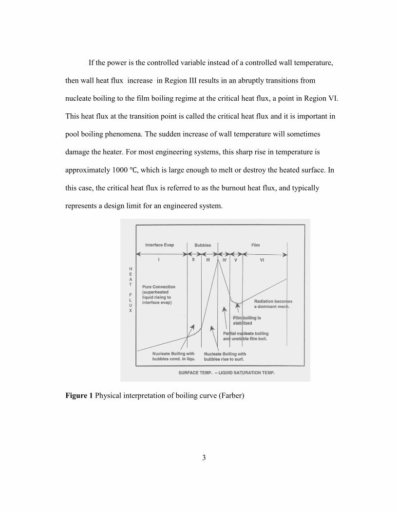
This present study seeks to contribute detailed visualization data on a pool
boiling experiments using HFE-7000. Particle Image Velocimetry (PIV) was used to
measure the time resolved whole field liquid velocity. Bubble dynamic parameters such
as nucleation site density, bubble departure diameter, contact angles and frequency were
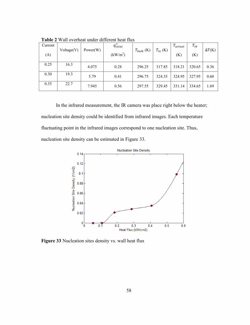
obtained in shadowgraphy measurements. Infrared thermometry with an IR camera was
used for observation of temperature fluctuations of nucleation sites. The experiments
were taken for the heat flux from 0.042 kW/m2 to 0.266 kW/m2, six experimental
conditions in total.
To provide a supplementary description of heat transfer mechanism, a novel
3.1.3 Visualization System .......................................................................... 29 3.1.4 Heating Element Design ..................................................................... 31 3.1.5 Power Supply and Working Fluid and Seeding Particles ................... 36 3.2 Experiments Procedure ............................................................................... 37
4. DATA PROCESSING AND RESULTS..................................................................... 40
4.1 PIV Data Processing and Results ................................................................ 40 4.2 Bubble Shadowgraphy Data Process and Results ....................................... 45 4.2.1 Data Analysis Process ........................................................................ 45 4.2.2 Results Discussion .............................................................................. 52 4.3 Infrared Measurement Results Analysis ..................................................... 55
5. RICM MEASUREMENT AND IMAGE PROCESSING .......................................... 59
5.1 RICM Test Facility ...................................................................................... 59 5.2 Image Process and Height/Shape Reconstruction ....................................... 61 5.2.1 Min/Max Method ............................................................................... 62 5.2.2 The Refractive Index Method ............................................................. 63 5.3 Height Reconstruction with Known Symmetric Shape ............................... 64 5.4 RICM Images Results and Discussion ........................................................ 67
Figure 5 Temperature distribution through ITO heater .......................................... 22
Figure 6 IR calibration experiment setup ............................................................... 23
Figure 7 IR calibration correlation ......................................................................... 23
Figure 8 Temperature difference through the ITO heater....................................... 24
Figure 9 The schematic of pool boiling facility ...................................................... 26
Figure 10 Photograph of pool boiling facility .......................................................... 26
Figure 11 FLIR systems, SC8200 IR camera ........................................................... 30
Figure 12 ITO heater schematic graph ..................................................................... 31
Figure 13 Infrared camera picture of the ITO heater ................................................ 33
Figure 14 Temperature profile of x axis ................................................................... 33
Figure 15 Improved heater temperature field ........................................................... 34
Figure 16 Temperature profile along x axis ............................................................. 34
Figure 17 Transmissivity spectrum of borosilicate glass substrate from Bayview Optics. Inc ................................................................................. 35
Figure 18 Transmissivity spectrum of ITO from Bayview Optics. Inc .................... 36
viii
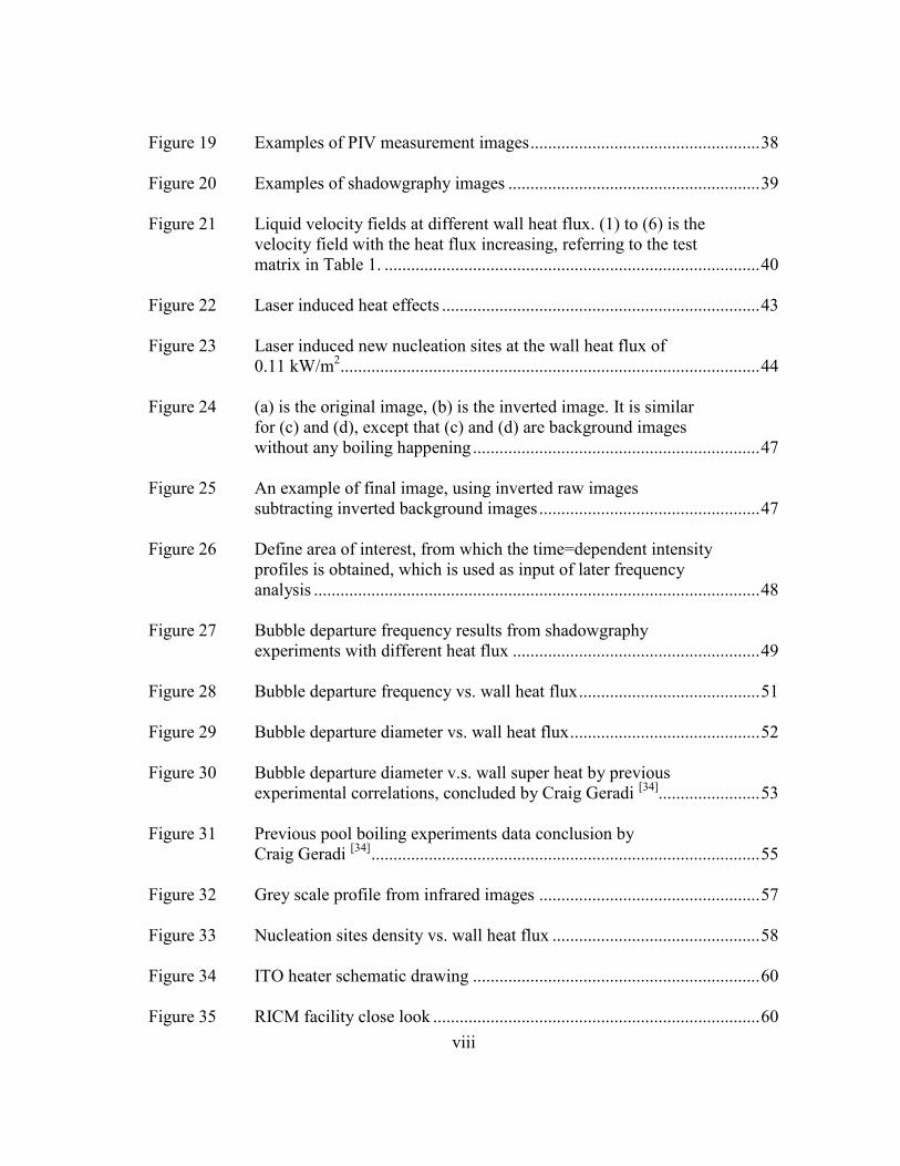
Figure 19 Examples of PIV measurement images .................................................... 38
Figure 20 Examples of shadowgraphy images ......................................................... 39
Figure 21 Liquid velocity fields at different wall heat flux. (1) to (6) is the velocity field with the heat flux increasing, referring to the test matrix in Table 1. ..................................................................................... 40
Figure 23 Laser induced new nucleation sites at the wall heat flux of 0.11 kW/m2 ............................................................................................... 44
Figure 24 (a) is the original image, (b) is the inverted image. It is similar for (c) and (d), except that (c) and (d) are background images without any boiling happening ................................................................. 47
Figure 25 An example of final image, using inverted raw images subtracting inverted background images .................................................. 47
Figure 26 Define area of interest, from which the time=dependent intensity profiles is obtained, which is used as input of later frequency analysis ..................................................................................................... 48
Figure 27 Bubble departure frequency results from shadowgraphy experiments with different heat flux ........................................................ 49
Figure 28 Bubble departure frequency vs. wall heat flux ......................................... 51
Figure 30 Bubble departure diameter v.s. wall super heat by previous experimental correlations, concluded by Craig Geradi [34]....................... 53
Figure 31 Previous pool boiling experiments data conclusion by Craig Geradi [34] ........................................................................................ 55
Figure 32 Grey scale profile from infrared images .................................................. 57
Figure 33 Nucleation sites density vs. wall heat flux ............................................... 58
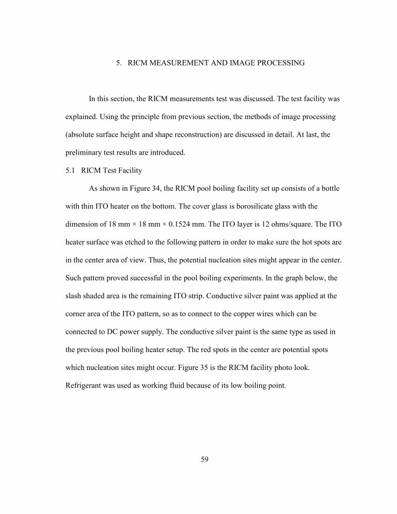
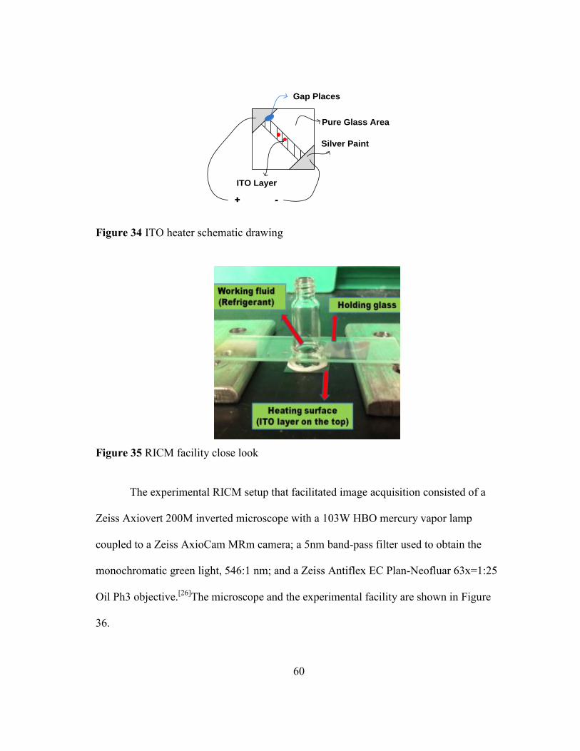
Figure 34 ITO heater schematic drawing ................................................................. 60
Figure 35 RICM facility close look .......................................................................... 60
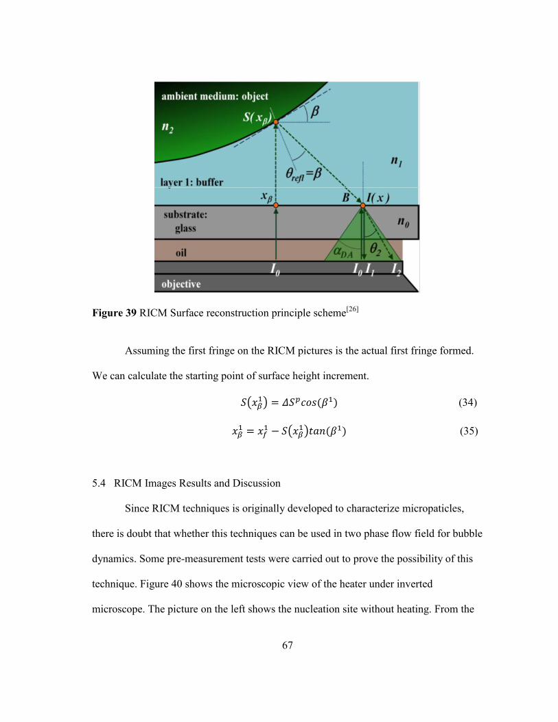
Figure 40 Background picture of nucleation site ...................................................... 68
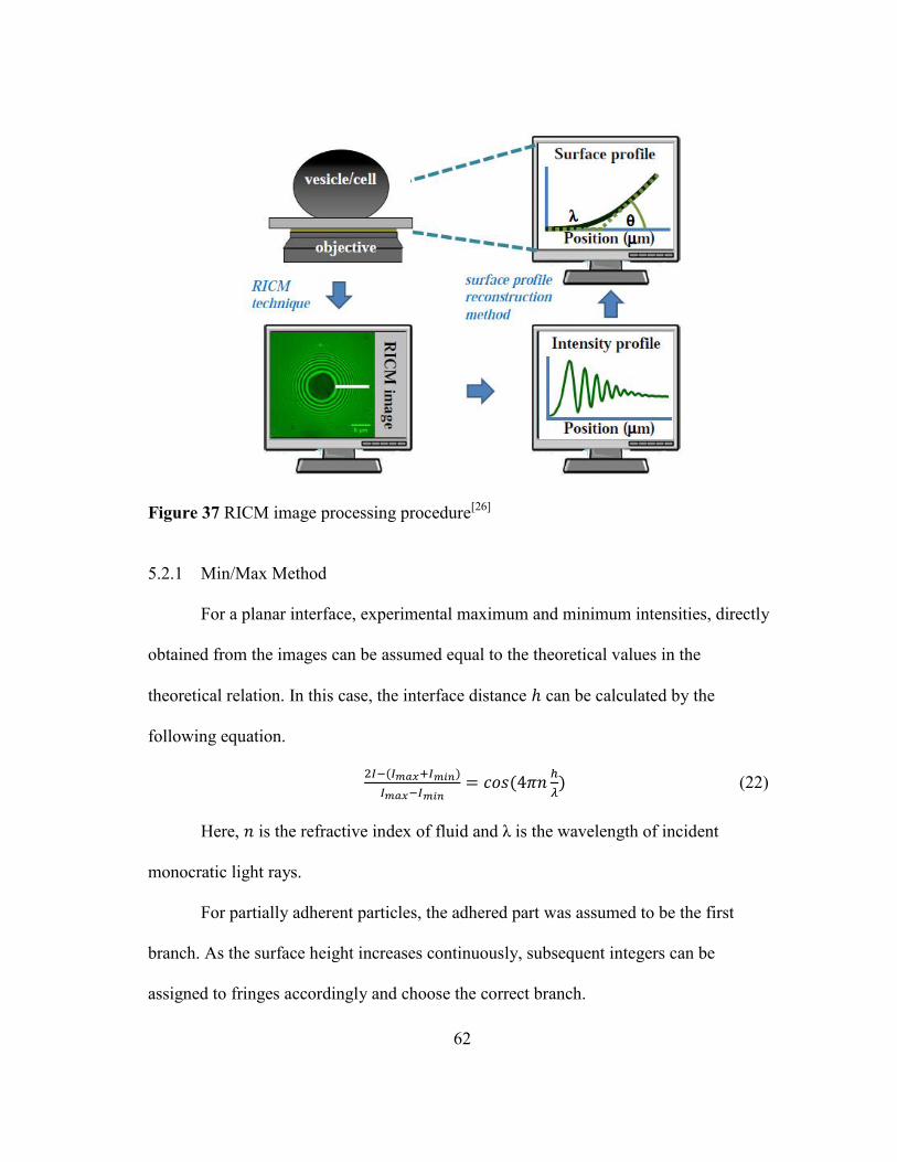
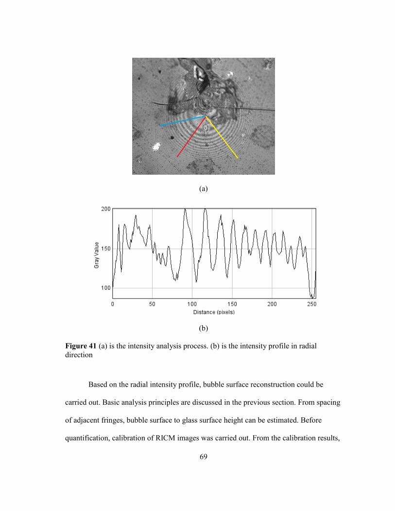
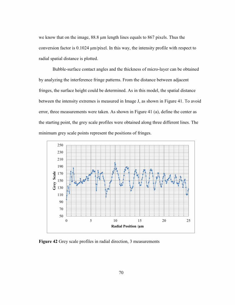
Figure 41 (a) is the intensity analysis process. (b) is the intensity profile in radial direction ..................................................................................... 69
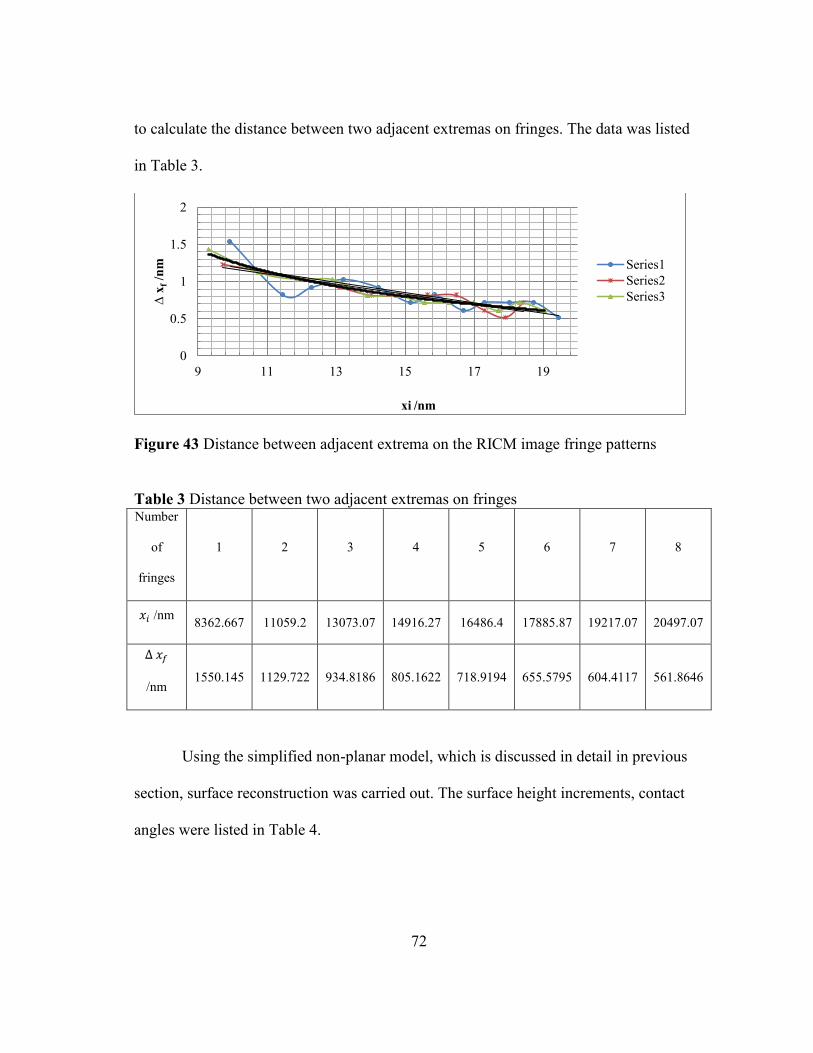
Figure 43 Distance between adjacent extrema on the RICM image fringe patterns ..................................................................................................... 72
was used to obtain detailed information on bubble dynamic parameters on the
microscopic scale. RICM is a technique originally developed to characterize the
adhesion of particle to glass surface. When a monochromatic light incident from the
bottom of the objects, it will interfere with the reflected light ray from the surface of the
object, forming interference fringes. This is how the RICM images are formed. In this
case, inducing monochromatic light from the bottom of the heating surface, light rays
reflected from the surface of the bubble and the heating surface will interfere and form
fringes. After an approximated fringe spacing analysis, the bubble geometry could be
obtained.
In this section, the basic principal of RICM measurements together with the
method of image processing (absolute surface height and shape reconstruction) is
discussed in detail.
17
2.2.1 RICM Theory
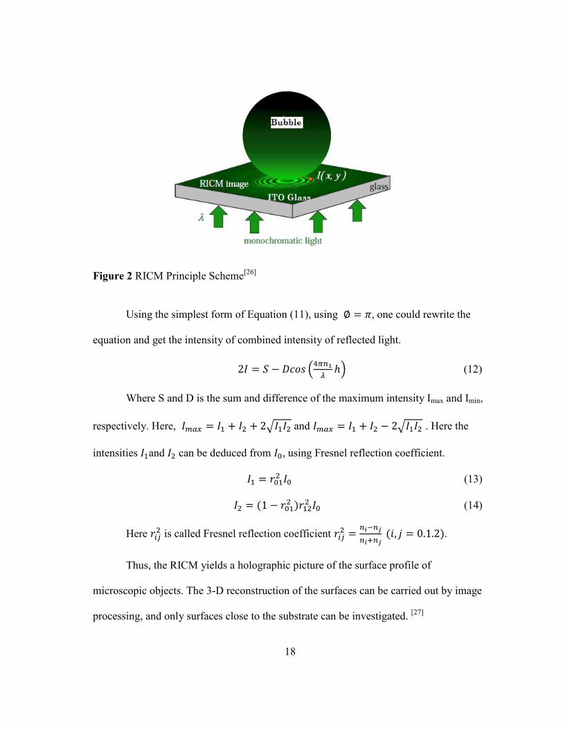
The optical theoretical basis for RICM technique is shown in Figure 2 . When a
monochromatic light incident from the bottom of the objects, it will interfere with the
reflected light ray from the surface of the object, forming interference fringes. From the
figure, we know that when a monochromatic beam of light incident from the bottom
of the plate, there will be two rays of reflection light. First the glass/medium interface
will reflect part of the light, gives the ray, ; while the transmitted ray will then be
reflected at the surface of the object, forming ray . and will interfere and combine
to a total intensity . The intensity of is described by the following equation.
√ ( ) (11)
Where,
⁄ and is the phase change, ( ) is the height between the
bubble and glass substrate at lateral position( ). The figure below shows the intensity
profiles on the glass substrate, which in case of pool boiling bubbles are concentric
fringes.
18
Figure 2 RICM Principle Scheme[26]
Using the simplest form of Equation (11), using , one could rewrite the
equation and get the intensity of combined intensity of reflected light.
(
) (12)
Where S and D is the sum and difference of the maximum intensity Imax and Imin,
respectively. Here, √ and √ . Here the
intensities and can be deduced from , using Fresnel reflection coefficient.
(13)
( )
(14)
Here is called Fresnel reflection coefficient
( ).
Thus, the RICM yields a holographic picture of the surface profile of
microscopic objects. The 3-D reconstruction of the surfaces can be carried out by image
processing, and only surfaces close to the substrate can be investigated. [27]
19
Oil
Glass substrate
Objective
Image Processing
Bubble
θ1
θ0 θ1
n0
n1
I2
I1
n2
Objective Lens
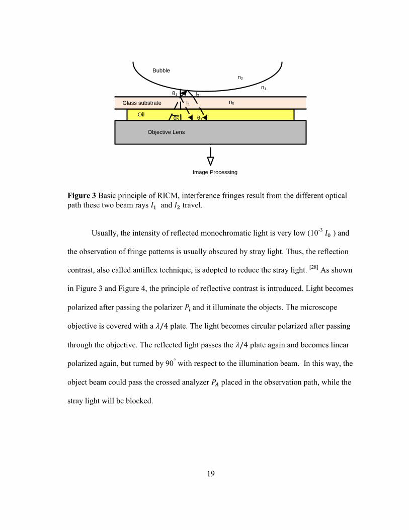
Figure 3 Basic principle of RICM, interference fringes result from the different optical path these two beam rays and travel.
Usually, the intensity of reflected monochromatic light is very low (10-3 ) and
the observation of fringe patterns is usually obscured by stray light. Thus, the reflection
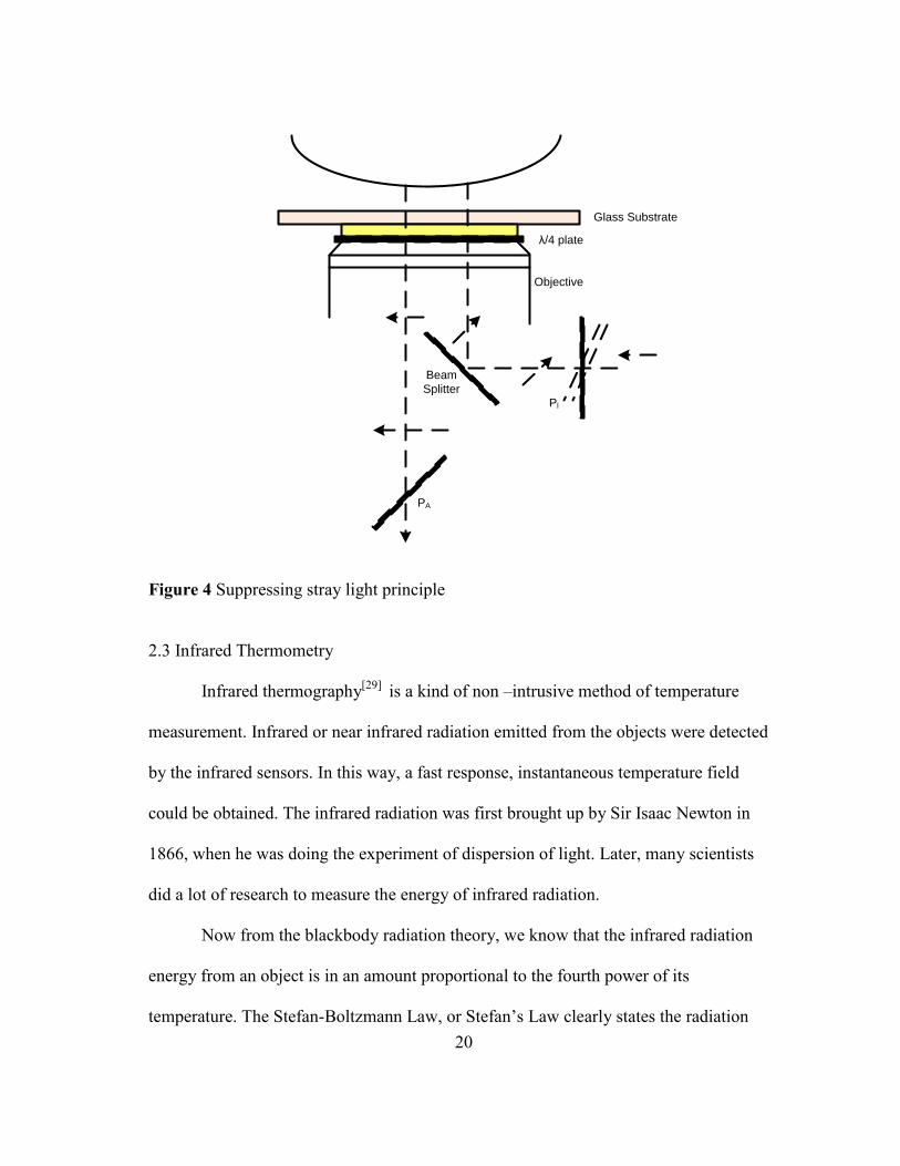
contrast, also called antiflex technique, is adopted to reduce the stray light. [28] As shown
in Figure 3 and Figure 4, the principle of reflective contrast is introduced. Light becomes
polarized after passing the polarizer and it illuminate the objects. The microscope
objective is covered with a plate. The light becomes circular polarized after passing
through the objective. The reflected light passes the plate again and becomes linear
polarized again, but turned by 90° with respect to the illumination beam. In this way, the
object beam could pass the crossed analyzer placed in the observation path, while the
stray light will be blocked.
20
λ/4 plate
Objective
Beam
SplitterPl
PA
Glass Substrate
Figure 4 Suppressing stray light principle
2.3 Infrared Thermometry
Infrared thermography[29] is a kind of non –intrusive method of temperature
measurement. Infrared or near infrared radiation emitted from the objects were detected
by the infrared sensors. In this way, a fast response, instantaneous temperature field
could be obtained. The infrared radiation was first brought up by Sir Isaac Newton in
1866, when he was doing the experiment of dispersion of light. Later, many scientists
did a lot of research to measure the energy of infrared radiation.
Now from the blackbody radiation theory, we know that the infrared radiation
energy from an object is in an amount proportional to the fourth power of its
temperature. The Stefan-Boltzmann Law, or Stefan’s Law clearly states the radiation
21
energy flux rate from blackbody with absolute temperature , as shown in
above1Equation (15).
(15) This is the foundation of infrared thermometry. In the real world, in order to
calculate the infrared energy emitted using blackbody radiation theory, the parameter
“emissivity” is introduced as a correction. Emissivity is a ratio of gray body emission to
that from a blackbody emission at the same temperature. Here, the emissivity of the gray
body is assumed constant with respect to wavelength.
When the object was viewed by the infrared camera, objects with different
temperature will emit infrared light with different energy and different wavelength, so
that the infrared camera could easily discriminate these objects. With a certain frame
rate, the infrared camera could capture the dynamic process of temperature profiles of
area of interest.
In this work, a SC8200 infrared camera from FLIR system., Inc, was used. This
camera has the resolution of 1024×1024, and the maximum frame rate of 132 Hz with
full window. If the measuring window is reduced, the frame rate can be increased. The
temperature within the range of -20 to 500 (-4 to 932 ).
It is obvious that the measurement value from IR camera cannot be used as the
object actual temperature, because of the error due to variation of emissivity, reflectivity,
and transmissivity of ITO-heater. More importantly, in the pool boiling experiments, IR
camera was measuring the glass side temperature. Due to conduction through the glass
22
and convection heat loss on the glass side, there will be a temperature drop through the
glass, as shown in Figure 5.
Tambient
Tinside
Glass
ITO Layer
Figure 5 Temperature distribution through ITO heater
In order to infer the actual temperature on the surface of ITO-heater, the
correlation from a series of simple experiments were estimated. The temperature range
of interest is from 30 to 70 . By comparing the measurements results from E-type
thermocouples and the experimental values from IR camera, the correlation is
concluded. In this test, IR camera was set at a frame rate of 131.5 Hz with the spatial
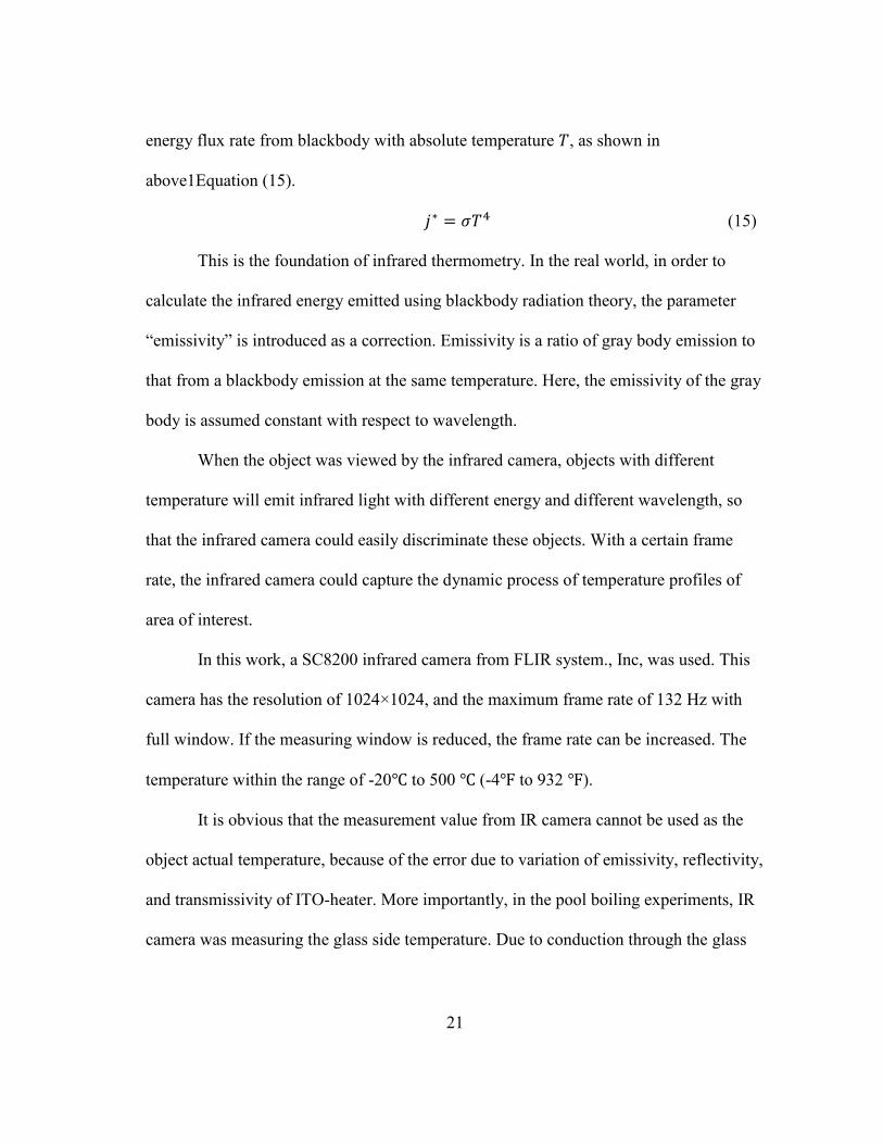
resolution of 1024 ×1024. The experimental set up is shown in Figure 1. The IR camera
was placed in front of a ITO heater. The heater was connected to a DC power supply. E-
type thermocouples was used to measure the real temperature of heater surface.
23
Figure 6 IR calibration experiment setup
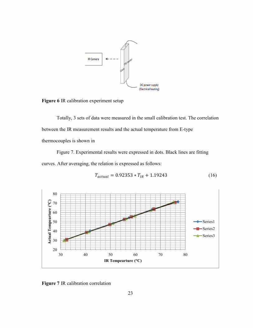
Totally, 3 sets of data were measured in the small calibration test. The correlation
between the IR measurement results and the actual temperature from E-type
thermocouples is shown in
Figure 7. Experimental results were expressed in dots. Black lines are fitting
curves. After averaging, the relation is expressed as follows:
(16)
Figure 7 IR calibration correlation
20
30
40
50
60
70
80
30 40 50 60 70 80
Act
ual T
empe
artu
re (°
C)
IR Tempearture (°C)
Series1
Series2
Series3
24
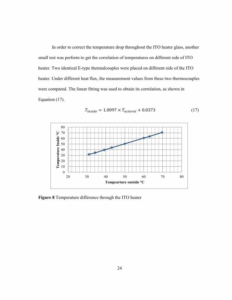
In order to correct the temperature drop throughout the ITO heater glass, another
small test was perform to get the correlation of temperatures on different side of ITO
heater. Two identical E-type thermalcouples were placed on different side of the ITO
heater. Under different heat flux, the measurement values from these two thermocouples
were compared. The linear fitting was used to obtain its correlation, as shown in
Equation (17).
(17)
Figure 8 Temperature difference through the ITO heater
01020304050607080
20 30 40 50 60 70 80
Tem
pera
ture
Ins
ide
°C
Tempearture outside °C
25
3. POOL BOILING EXPERIMENTS
In this chapter, the pool boiling facility was discussed in detail from the set up
stage to the experimental procedure. The fabrication of the ITO heater and how it is set
up in the facility is crucial for the success of the pool boiling experiments. In this
experiment, we started to gain some first experience about how to use the infrared
camera to capture the temperature field of heating surface. Moreover, a lot of experience
had been learned from setting up of the facility, which is valuable for future heat transfer
experiments, such as subcooled flow boiling experiments. The results of the test are
analyzed in the reminder of this thesis to give a picture of the pool boiling two phase
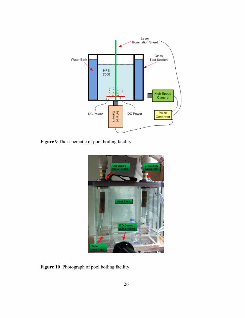
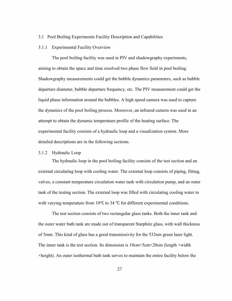
field. The schematic of pool boiling facility is shown in Figure 9, and a photograph of
the facility is in the following figure.
26
Figure 9 The schematic of pool boiling facility
Figure 10 Photograph of pool boiling facility
27
3.1 Pool Boiling Experiments Facility Description and Capabilities
3.1.1 Experimental Facility Overview
The pool boiling facility was used in PIV and shadowgraphy experiments,
aiming to obtain the space and time resolved two phase flow field in pool boiling.
Shadowgraphy measurements could get the bubble dynamics parameters, such as bubble
departure diameter, bubble departure frequency, etc. The PIV measurement could get the
liquid phase information around the bubbles. A high speed camera was used to capture
the dynamics of the pool boiling process. Moreover, an infrared camera was used in an
attempt to obtain the dynamic temperature profile of the heating surface. The
experimental facility consists of a hydraulic loop and a visualization system. More
detailed descriptions are in the following sections.
3.1.2 Hydraulic Loop
The hydraulic loop in the pool boiling facility consists of the test section and an
external circulating loop with cooling water. The external loop consists of piping, fitting,
valves, a constant temperature circulation water tank with circulation pump, and an outer
tank of the testing section. The external loop was filled with circulating cooling water to
with varying temperature from 10 to 34 for different experimental conditions.
The test section consists of two rectangular glass tanks. Both the inner tank and
the outer water bath tank are made out of transparent Starphire glass, with wall thickness
of 5mm. This kind of glass has a good transmissivity for the 532nm green laser light.
The inner tank is the test section. Its dimension is 10cm×5cm×20cm (length ×width
×height). An outer isothermal bath tank serves to maintain the entire facility below the
28
saturation temperature of the refrigerant (34 ) throughout the duration of each
experiment. The Novec 3M 7000 Fluid was chosen as the working fluid because of its
unique thermal and mechanical properties. All the component materials are chosen to be
compatible with the working fluid. The test chamber was designed at the atmospheric
pressure of 1 atm. The outer tank was used similar to the water bath, to keep the inner
test tank temperature constant for different experimental conditions. Loss of fluid in the
inner tank by evaporation is minimized by maintaining a quasi-seal on the top of the
tank. The top lid prevents most of the steam leakage, but it is loose enough to keep the
test tank at atmospheric pressure.
Energy for the pool boiling was provided by a borosilicate glass covered with
Indium-Tin-Oxide (ITO) layer. Only a strip area of approximate 142 mm2 is covered
with the ITO layer. Such pattern is to eliminate the bubbles from generating from the
side, enabling most of the nucleation sites are within the camera view. The reason why
such fabrication was adopted is discussed in the following section. The maximum
working temperature of the heater is approximately 200 . To reduce heat losses to the
environment, hard paper was used to cover the around the test facility. However, still,
the heat loss by radiation and convection is not negligible. Such loss is discussed in
detail in the reminder of the thesis. By connecting the ITO heater to the DC power
supply, from which a series of heat flux were achieved, from 0.042127 kW/m2 to the
maximum heat flux of 0.266493 kW/m2. By Joule heating, pool boiling occurred on the
surface of the ITO film.
29
To monitor the temperature of the heating surface and the bulk fluid temperature
in the pool, two K-type thermal couples are placed inside the test section pool. One is
placed near the heating surface; the other was in the bulk tank. Moreover, to record the
temperature fluctuation of the heater surface, infrared thermometry with IR camera was
used by measuring the infrared light intensity. Synchronized with the high speed camera
by pulse generator, the dynamic process of boiling was captured.
3.1.3 Visualization System
The visualization system consists of flow particles tracer, a high speed camera, a
high frequency, high power laser for PIV experiments, a halogen lamp for
shadowgraphy experiments, lenses and mirrors, other supportive tracks.
A kind of highly reflective silver coated particles was selected as the flow tracer
for PIV measurements. Such kind of particles has a density range of 1.39 to 1.41 g/cm3.
Such density range is preferred since it is almost the same with the working fluid of HFE
7000, which density is 1.4 g/cm3. When under heated situation, the particles would
suspend in the bulk fluid, tacking the movement of liquid phase. Its diameter is about
40µm. The illumination source for the PIV experiments is a 527nm laser source. In the
shadowgraphy experiment, the illumination source is a continuous halogen lamp.
The maximum frame rate of high speed camera is 7000 frames per second at a
maximum resolution of 800×600 pixels. The spatial resolution of the camera is µm/
pixel. In the PIV experiments, the high speed camera was synchronized with the laser
source through a pulse generator. The illumination source was provided by a twin pulsed
Nd-Yag laser with green light wavelength of 527 nm. Optical reflective mirror and
30
concave-convex lenses are used to convert the small circular beam from the laser source
into a thin sheet of light. In the experiment, the laser sheet is positioned through the mid-
plane of the tank from one side, shinning perpendicular to the ITO heater surface in
order to illuminate the particles above the heater. The camera was positioned
perpendicular in front of the tank compared to the laser sheet. The lenses, mirrors and
cameras are mounted to the movable tracks, so that their relative positions could be
adjusted for better focus onto the measurement region.
For the shadowgraphy measurements, similar the PIV video acquisition system,
the same high speed camera was used. Instead of high frequency laser beam source, a
continuous halogen lamp was used for illumination.
To acquire the temperature fluctuation profile of the ITO heater surface, an
infrared camera was used to measure IR intensity from the bottom of the pool boiling
facility. The IR camera was a SC8200 IR camera from FLIR systems, Inc, as shown in
Figure 11.
Figure 11 FLIR systems, SC8200 IR camera
31
3.1.4 Heating Element Design
In this facility, the transparent ITO heater was chosen. Boiling occurs on the
upward facing side of the ITO layer. The schematic and photograph of the heater is
shown in Figure 12.
Silver paint electrodes
ITO
Borosilicate glass substrate
Figure 12 ITO heater schematic graph
The ITO was deposited onto the borosilicate substrates. The substrate was 1.1
mm thick. The heater was made by Bayview Optics company in Maine, US. The ITO
layer deposited on the glass substrates has the resistance of 10 Ohms/Square with the
thickness of 1500 Angstroms. Usually, the actual resistance of the heater is slightly
higher which is due to slight difference in the manufactured ITO thickness and
properties.
As shown in the schematic figure of the ITO heater, silver electrodes were used
for connecting to the DC power supply. Because of the high thermal conductivity and
low electric resistance of the silver metal, the temperature hot spot will not be located at
the areas of the electrodes. At first, we attempted to deposit pure silver onto the ITO
surface to fabricate the electrodes. About 100 nm thick of silver was deposited onto the
32
ITO surface by metal evaporation technique. However, the pure silver layer is easily
peeled off the surface. Then we found an easier way to fabricate the electrodes. A
reliable conductive silver paint from Ted Pella, Inc. was applied. Leitsilber[30] is a fast
drying and has a flat surface texture, normally used in SEM specimens. The silver
content is 45%, with a resistance of 0.02-0.04 Ohms/Square. Its maximum surface
temperature is 120 . The silver paint can be easily applied to the ITO heater surface by
brush. Pre-tests have shown that the surface is smooth enough to eliminate cavities from
becoming potential nucleation sites.
As for the connection of the heater to the DC power supply, copper wires were
fixed onto the silver electrodes by double sided adhesive, electrically highly conductive
carbon tapes. Such kind of tape was specially designed for attaching samples to be
examined by SEM. Since the surface of the tape is porous, the silver paint was applied
on top of the tape after attaching the copper wire to the heater surface.
Small tests were performed using infrared camera to make sure the preferred
temperature profiles is achieved. Connecting to the DC power supply, the ITO heater
was placed in front of the IR camera. Figure 13 and Figure 14 shows the temperature
profile of heating surface. This is the profile when the ITO heater was glued to the
bottom of the inner test tank by UV epoxy.
33
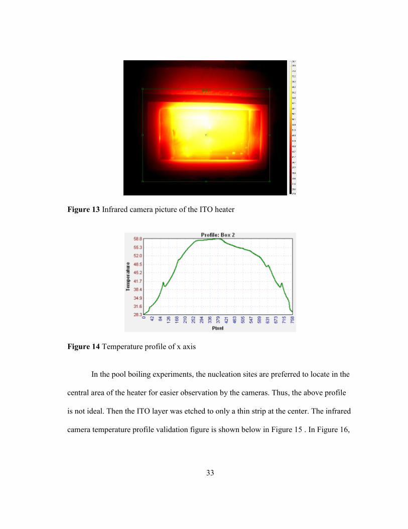
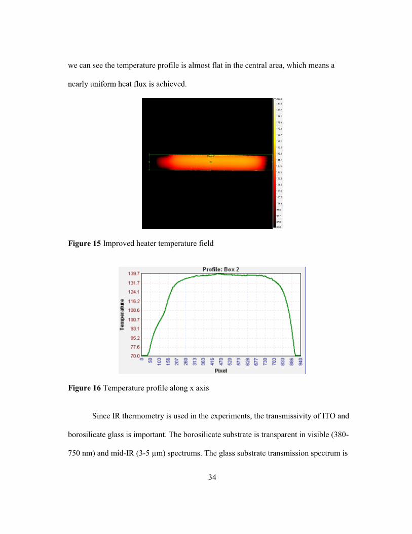
Figure 13 Infrared camera picture of the ITO heater
Figure 14 Temperature profile of x axis
In the pool boiling experiments, the nucleation sites are preferred to locate in the
central area of the heater for easier observation by the cameras. Thus, the above profile
is not ideal. Then the ITO layer was etched to only a thin strip at the center. The infrared
camera temperature profile validation figure is shown below in Figure 15 . In Figure 16,
34
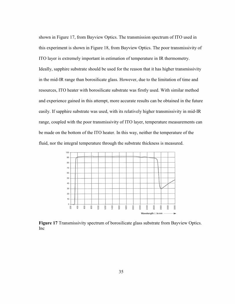
we can see the temperature profile is almost flat in the central area, which means a
nearly uniform heat flux is achieved.
Figure 15 Improved heater temperature field
Figure 16 Temperature profile along x axis
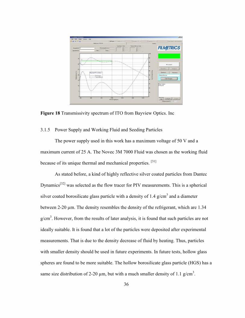
Since IR thermometry is used in the experiments, the transmissivity of ITO and
borosilicate glass is important. The borosilicate substrate is transparent in visible (380-
750 nm) and mid-IR (3-5 µm) spectrums. The glass substrate transmission spectrum is
35
shown in Figure 17, from Bayview Optics. The transmission spectrum of ITO used in
this experiment is shown in Figure 18, from Bayview Optics. The poor transmissivity of
ITO layer is extremely important in estimation of temperature in IR thermometry.
Ideally, sapphire substrate should be used for the reason that it has higher transmissivity
in the mid-IR range than borosilicate glass. However, due to the limitation of time and
resources, ITO heater with borosilicate substrate was firstly used. With similar method
and experience gained in this attempt, more accurate results can be obtained in the future
easily. If sapphire substrate was used, with its relatively higher transmissivity in mid-IR
range, coupled with the poor transmissivity of ITO layer, temperature measurements can
be made on the bottom of the ITO heater. In this way, neither the temperature of the
fluid, nor the integral temperature through the substrate thickness is measured.
Figure 17 Transmissivity spectrum of borosilicate glass substrate from Bayview Optics. Inc
36
Figure 18 Transmissivity spectrum of ITO from Bayview Optics. Inc
3.1.5 Power Supply and Working Fluid and Seeding Particles
The power supply used in this work has a maximum voltage of 50 V and a
maximum current of 25 A. The Novec 3M 7000 Fluid was chosen as the working fluid
because of its unique thermal and mechanical properties. [31]
As stated before, a kind of highly reflective silver coated particles from Dantec
Dynamics[32] was selected as the flow tracer for PIV measurements. This is a spherical
silver coated borosilicate glass particle with a density of 1.4 g/cm3 and a diameter
between 2-20 µm. The density resembles the density of the refrigerant, which are 1.34
g/cm3. However, from the results of later analysis, it is found that such particles are not
ideally suitable. It is found that a lot of the particles were deposited after experimental
measurements. That is due to the density decrease of fluid by heating. Thus, particles
with smaller density should be used in future experiments. In future tests, hollow glass
spheres are found to be more suitable. The hollow borosilicate glass particle (HGS) has a
same size distribution of 2-20 µm, but with a much smaller density of 1.1 g/cm3.
37
3.2 Experiments Procedure
The PIV and bubble shadowgraphy measurements were carried out for 6
different heat flux conditions, from 0.042 kW/m2 to 0.266 kW/m2. In the PIV
measurements, the visualization system is equipped with a laser as an illumination
source for the high-resolution/high-speed that is to be placed perpendicular to the laser
sheet plane.
In the PIV measurements, the camera was positioned to focus the surface of the
ITO heater. The camera was synchronized with a high energy laser. The laser sheet is
1mm thick, used for illumination. The camera frame rate was set at 2000 frames/s, with
an exposure time of 2 µs. Each image acquired consisted of 600×800 pixels. For each
pixel in the image, it represents 0.2822 mm in realtity. For each different heat flux, water
bath temperature was kept at 20 . For each case, 4398 pictures were acquired. The
experimental matrix is shown in Table 1.
To ensure the inner pool bulk temperature is below the boiling point of working
fluids, T-type thermocouples were used as validation.
The heater energy was provided by a DC power supply, with varying voltage and
current. Due to heat loss from the bottom of the ITO heater, the actual heat flux from the
inner surface of the pool tank should be modified. Assume that the heat loss from the
outer surface heater is purely due to free air convection. Radiation is neglected since
temperature difference between the heater and environment is not large. And assume the
heat convection transfer coefficient is constant. So, the actual wall heat flux was estimate
using the following assumption:
38
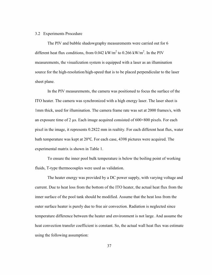
( ) (18)
Table 1 Test matrix of the PIV and shadowgraphy experiments
Current (A) Voltage(V) Power(W)
(kW/m2) (K) (K)
(kW/m2)
0.10 7.7 0.77 0.054127092 301.45 300.25 0.042127
0.15 10.2 1.53 0.107551236 306.25 300.25 0.047551
0.20 13.1 2.62 0.184172704 312.45 300.25 0.062172
0.25 16.3 4.075 0.28645182 317.85 300.25 0.110451
0.30 19.3 5.79 0.407007617 324.35 300.25 0.166007
0.35 22.7 7.945 0.55849318 329.45 300.25 0.266493
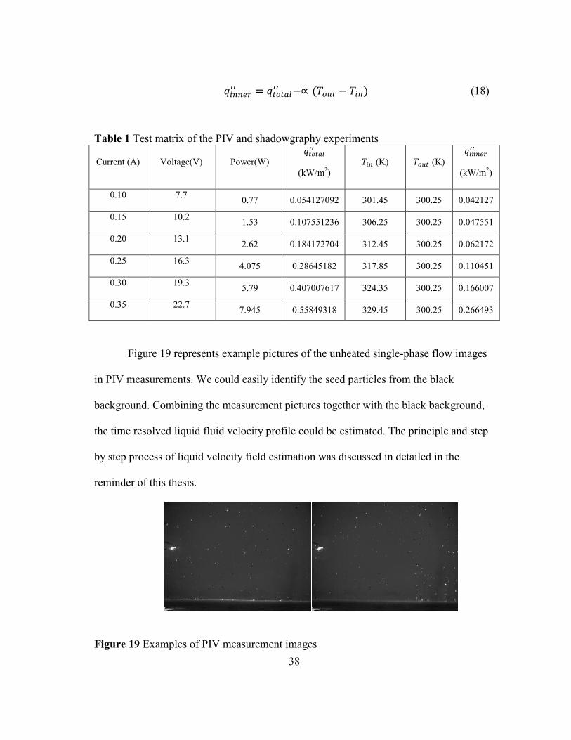
Figure 19 represents example pictures of the unheated single-phase flow images
in PIV measurements. We could easily identify the seed particles from the black
background. Combining the measurement pictures together with the black background,
the time resolved liquid fluid velocity profile could be estimated. The principle and step
by step process of liquid velocity field estimation was discussed in detailed in the
reminder of this thesis.
Figure 19 Examples of PIV measurement images
39
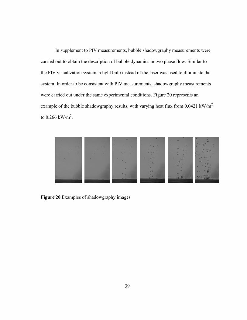
In supplement to PIV measurements, bubble shadowgraphy measurements were
carried out to obtain the description of bubble dynamics in two phase flow. Similar to
the PIV visualization system, a light bulb instead of the laser was used to illuminate the
system. In order to be consistent with PIV measurements, shadowgraphy measurements
were carried out under the same experimental conditions. Figure 20 represents an
example of the bubble shadowgraphy results, with varying heat flux from 0.0421 kW/m2
to 0.266 kW/m2.
Figure 20 Examples of shadowgraphy images
40
4. DATA PROCESSING AND RESULTS
4.1 PIV Data Processing and Results
For each of the 6 different experimental conditions, a clip of video was recorded.
The water bath temperature was kept at 20 . To ensure the pool bulk temperature is
below the boiling point of refrigerant, T-type thermocouples measurement results were
listed in Table 1. Each video tape was then broken down to 4398 frames of pictures, with
the time interval of 0.5 ms between two consecutive pictures. A home developed
program was used for analysis. The principle of the software was discussed in detail in
the previous section.
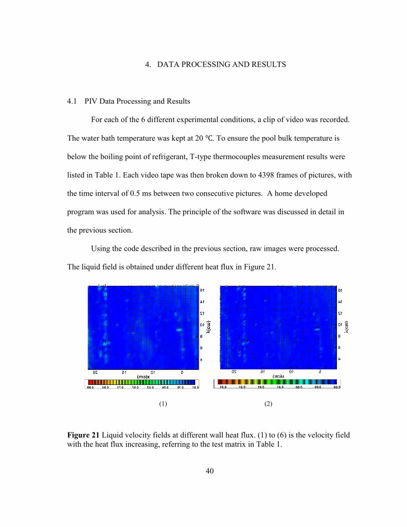
Using the code described in the previous section, raw images were processed.
The liquid field is obtained under different heat flux in Figure 21.
(1) (2)
Figure 21 Liquid velocity fields at different wall heat flux. (1) to (6) is the velocity field with the heat flux increasing, referring to the test matrix in Table 1.
41
(3) (4)
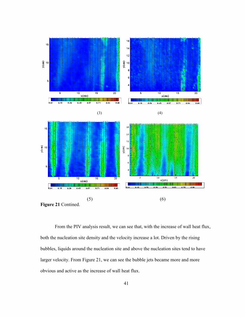
(5) (6) Figure 21 Contined.
From the PIV analysis result, we can see that, with the increase of wall heat flux,
both the nucleation site density and the velocity increase a lot. Driven by the rising
bubbles, liquids around the nucleation site and above the nucleation sites tend to have
larger velocity. From Figure 21, we can see the bubble jets became more and more
obvious and active as the increase of wall heat flux.
42
The velocity field results are not very satisfactory. The vortex and other
characteristics cannot be observed in the above figures. The main reason behind this is
that the particle tracers are not suitable for this experimental condition. The density of
this kind of silver coated hollow glass spheres is 1.4 g/cm3, the same with refrigerant.
However, when heated, the density of refrigerant decreases, resulting some portion of
particle tracers deposited onto the tank bottom. And the remaining particle tracers were
not following the fluid motions very closely. Later experiments showed that with lighter
particles, e.g. hollow borosilicate glass spheres, the PIV images are more satisfactory.
Moreover, in this experiment, the camera was set at a frame rate of 2000 frames/s, which
is too high for this low heat flux. From later image processing, I noticed that during
single time interval, , the particle tracers barely move. This frame rate was chosen
based on previous PIV experiments experience. However, in the past tests, the fluid
motion is usually much active than pool boiling condition. This induced very large error
in the data analysis. So in later experiments, 500 frames/s is fast enough for the PIV
measurements.
Since the working fluid is refrigerant, its boiling point is very low. Thus, the
power induced by the laser sheet should be considered in estimating the heat flux onto
the pool. When laser is induced into the glass tank, more heat will be induced into the
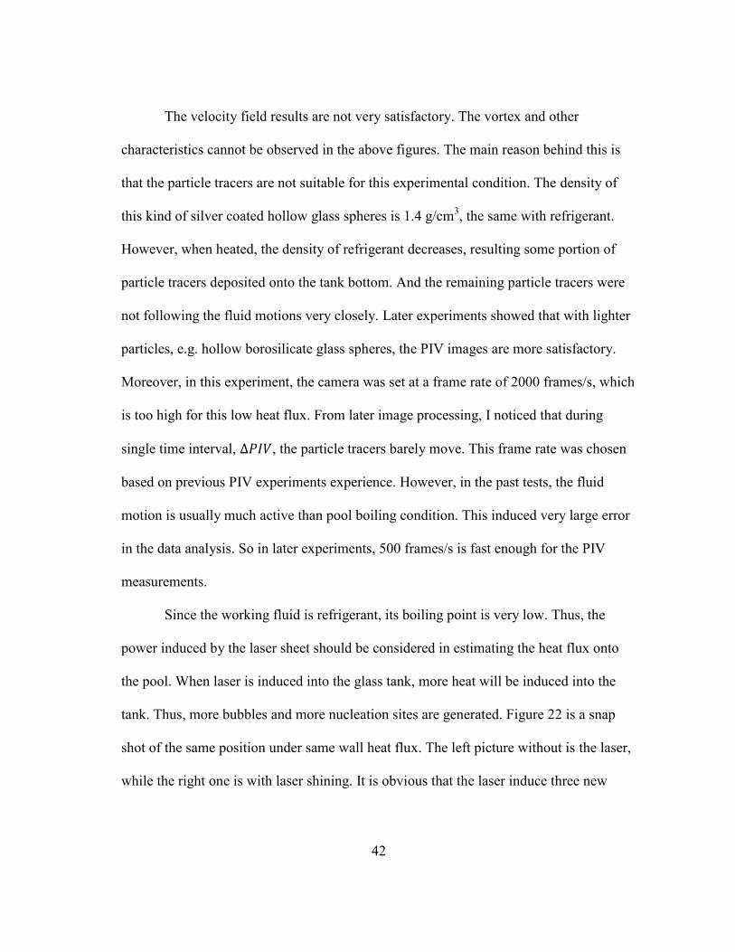
tank. Thus, more bubbles and more nucleation sites are generated. Figure 22 is a snap
shot of the same position under same wall heat flux. The left picture without is the laser,
while the right one is with laser shining. It is obvious that the laser induce three new
43
nucleation sites. This effect should be taken into consideration especially under
subcooled conditions when wall heat flux is low.
Figure 22 Laser induced heat effects
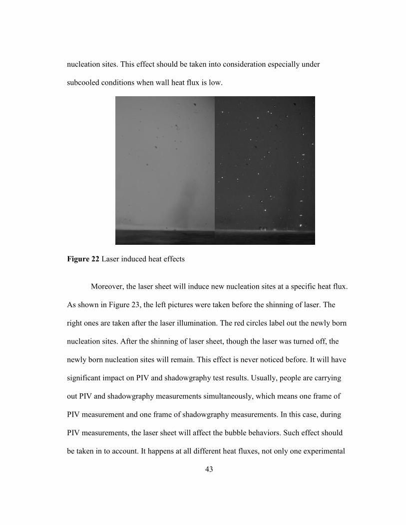
Moreover, the laser sheet will induce new nucleation sites at a specific heat flux.
As shown in Figure 23, the left pictures were taken before the shinning of laser. The
right ones are taken after the laser illumination. The red circles label out the newly born
nucleation sites. After the shinning of laser sheet, though the laser was turned off, the
newly born nucleation sites will remain. This effect is never noticed before. It will have
significant impact on PIV and shadowgraphy test results. Usually, people are carrying
out PIV and shadowgraphy measurements simultaneously, which means one frame of
PIV measurement and one frame of shadowgraphy measurements. In this case, during
PIV measurements, the laser sheet will affect the bubble behaviors. Such effect should
be taken in to account. It happens at all different heat fluxes, not only one experimental
44
condition. Figure 23 only shows the experimental condition when heat flux is at 0.11
kW/m2.
Figure 23 Laser induced new nucleation sites at the wall heat flux of 0.11 kW/m2
To quantify the amount of heat induced by the laser, and reduce the error of wall
heat flux, laser power quantification experiments should be carried out. The laser
induced heat flux effect was not noticed only after the pool boiling PIV measurements.
This is the first time we noticed such error. In the previous test, either the heat flux is
high enough to cover the laser effect, or the working fluid has a much higher boiling
point, such as water. Aware of this influence, laser power quantification tests were
carried out for the subcooled flow boiling experiments.
From the experiments done by my colleagues, the average energy deposition rate
by the laser sheet to the pool of refrigerant is estimated. From the results, we know that
the estimated deposition ratio is approximately 0.3164. The heat induced by laser is
calculated by
( ) ( )
45
After simple math, it shows that the amount of heat induced by laser sheet is
comparable with the wall heat flux. Such quantification tests are necessary.
4.2 Bubble Shadowgraphy Data Process and Results
4.2.1 Data Analysis Process
The image processing software Image J was used in processing of shadowgraphy
images. Image J is a Java based imaging processing and analysis software. This software
can display, edit, process 8-bit color and grayscale, 16-bit integer and 32-bit floating
point images. It can read many image formats including TIFF, PNG, GIF, JPEG, BMP,
DICOM, FITS, as well as raw formats. Image J supports image stacks, a series of images
that share a single window, and it is multithreaded, so time-consuming operations can be
performed in parallel on multi-CPU hardware. Image J can calculate area and pixel value
statistics of user-defined selections and intensity threshold objects. It can measure
distances and angles. It can create density histograms and line profile plots. It supports
standard image processing functions such as logical and arithmetical operations between
edge detection and median filtering. It does geometric transformations such as scaling,
rotation and flips. The program supports any number of images simultaneously, limited
only by available memory.[33]
The analysis process of shadowgraphy raw data includes three major steps, as
described as follows.
First, videos got from the high speed camera were broken down to raw images,
with the windows 8-bit grayscale BMP format. This raw image includes both the
46
bubbles and background. In the raw image, the background is brighter than the bubble
area. Light from the lamp shines onto the test section, the camera captured the bubble
shadow area. However, bubble areas are preferred to be the brighter area, for easier
image processing. Thus, the raw images were firstly being reverted, as shown in Figure
24. This image processing step was used for every image including the background
images. To reduce error from background images, a few background images of the same
position were taken. The images shown in Figure 24 are the average of all the
background images. In this work, 100 background images were used to obtain the
average background. A background image was taken without any heating or boiling.
Then, images with only the bubbles were obtained by subtracting the background
images from the raw images. The image becomes bright bubble shapes with black
background. This is much easier for future image analysis. The final images become
bright bubble with black background. In this way, the only intensity the software detects
comes from bubbles. An example of the final images is shown in Figure 24.
47
Figure 24 (a) is the original image, (b) is the inverted image. It is similar for (c) and (d), except that (c) and (d) are background images without any boiling happening
Figure 25 An example of final image, using inverted raw images subtracting inverted background images
48
Using Image J, an area of interest was defined in the image stack window. Then
the area gray scale profiles with respective to time was obtained, shown in Figure 26.
From a stack of images, grey scale intensity in the area of interest fluctuates with respect
with time. When the bubble passes through the area, the grey scale value will hit a peak.
After the bubble passed, its grey scale will decrease to the minimum value. The change
of grey scale reflects the bubble generation frequency. Also, from the slope of the rising
peaks, bubble growth time and bubble departure time could be roughly estimated.
Figure 26 Define area of interest, from which the time=dependent intensity profiles is obtained, which is used as input of later frequency analysis
The intensity profile was used as an input signal of the MATLAB program. Then
the time-frequency analysis was carried out. By Fourier analysis, the gray scale profile
function of time was converted into a new function of frequency. This function of
frequency is also referred to as frequency spectrum of the original grey scale function.
By fast Fourier transform (FFT), a dominate frequency could be found from the original
signal. After the FFT analysis by MATLAB, a frequency spectrum was obtained, from
49
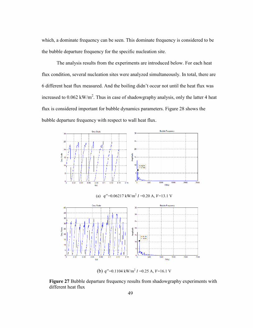
which, a dominate frequency can be seen. This dominate frequency is considered to be
the bubble departure frequency for the specific nucleation site.
The analysis results from the experiments are introduced below. For each heat
flux condition, several nucleation sites were analyzed simultaneously. In total, there are
6 different heat flux measured. And the boiling didn’t occur not until the heat flux was
increased to 0.062 kW/m2. Thus in case of shadowgraphy analysis, only the latter 4 heat
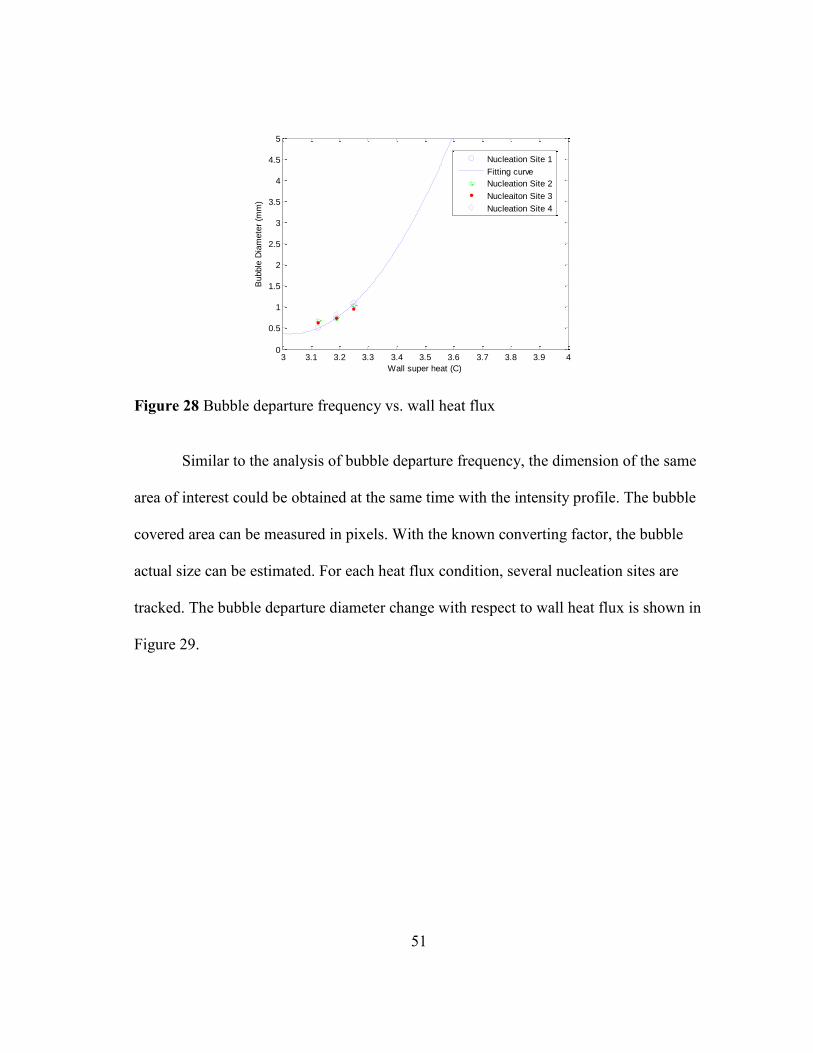
flux is considered important for bubble dynamics parameters. Figure 28 shows the
bubble departure frequency with respect to wall heat flux.
(a) =0.06217 kW/m2 =0.20 A, =13.1 V
(b) =0.1104 kW/m2 =0.25 A, =16.1 V
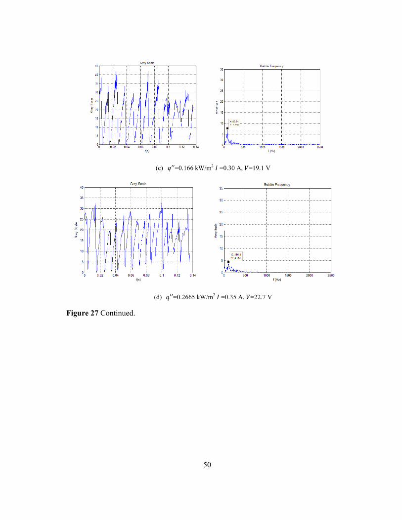
Figure 27 Bubble departure frequency results from shadowgraphy experiments with different heat flux
50
(c) =0.166 kW/m2 =0.30 A, =19.1 V
(d) =0.2665 kW/m2 =0.35 A, =22.7 V
Figure 27 Continued.
51
Figure 28 Bubble departure frequency vs. wall heat flux
Similar to the analysis of bubble departure frequency, the dimension of the same
area of interest could be obtained at the same time with the intensity profile. The bubble
covered area can be measured in pixels. With the known converting factor, the bubble
actual size can be estimated. For each heat flux condition, several nucleation sites are
tracked. The bubble departure diameter change with respect to wall heat flux is shown in
Figure 29.
3 3.1 3.2 3.3 3.4 3.5 3.6 3.7 3.8 3.9 40
0.5
1
1.5
2
2.5
3
3.5
4
4.5
5
Wall super heat (C)
Bubble
Dia
mete
r (m
m)
Nucleation Site 1
Fitting curve
Nucleation Site 2
Nucleaiton Site 3
Nucleation Site 4
52
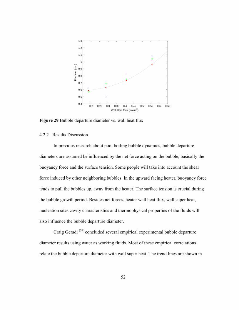
Figure 29 Bubble departure diameter vs. wall heat flux
4.2.2 Results Discussion
In previous research about pool boiling bubble dynamics, bubble departure
diameters are assumed be influenced by the net force acting on the bubble, basically the
buoyancy force and the surface tension. Some people will take into account the shear
force induced by other neighboring bubbles. In the upward facing heater, buoyancy force
tends to pull the bubbles up, away from the heater. The surface tension is crucial during
the bubble growth period. Besides net forces, heater wall heat flux, wall super heat,
nucleation sites cavity characteristics and thermophysical properties of the fluids will
also influence the bubble departure diameter.
Craig Geradi [34] concluded several empirical experimental bubble departure
diameter results using water as working fluids. Most of these empirical correlations
relate the bubble departure diameter with wall super heat. The trend lines are shown in
0.2 0.25 0.3 0.35 0.4 0.45 0.5 0.55 0.6 0.650.4
0.5
0.6
0.7
0.8
0.9
1
1.1
1.2
1.3
Wall Heat Flux (kW/m2)
Dia
mete
r (m
m)
53
Figure 30 Bubble departure diameter v.s. wall super heat by previous experimental correlations, concluded by Craig Geradi [34]
By comparing these empirical models with my own experimental data, we found
that the experimental data fits the Ruckenstein model[6] the best. In this model, besides
the buoyancy forces and surface tension force, the shear forces induced by departure of
neighboring bubbles are also considered. The bubble departure diameter was related
with Jakob number, Ja. Ja is a non-dimensional number widely used in describing the
phase transition phenomena. The correlation is expressed in Equation (19).
(
( )
)
( ) (19)
As in many articles, the bubble departure frequency is normally defined as the
reciprocal of cycle time . Here is the sum of the growth time, and the wait
time .[35]
( )⁄ (20)
54
Waiting time depends on the temperature field in both the solids and the liquid in
vicinity of the nucleation site. Growth time depends on the bubble and its departure
diameter. It is very difficult to develop a model to predict the bubble departure
frequency. It is associated with bubble diameter and wait time, growth time. The latter
parameters are affected by the temperature field in two phase flow. Usually, it is
assumed that bubble departure time is small enough compared to bubble growth time, so
is neglected.
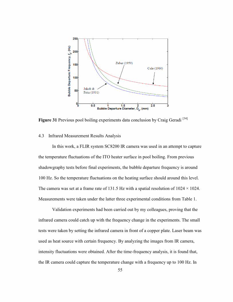
In this way, it is acknowledged that bubble departure frequency is determined by
the bubble departure diameters. However, the departure frequency varies from
nucleation sites to nucleation sites. A mean bubble departure frequency was usually
estimated at given wall heat flux or wall super heat. Craig Geradi [34] concluded several
empirical experimental bubble departure frequency results in Figure 31. Zuber’s
expression in 1959 is the most commonly used one. [36]
( )
⁄ (21)
After comparing my experimental data with previous models, it is found that the
frequency v.s. diameter trends fit the Zuber correlation the best. However, there are
noticeable discrepancy between experimental data and previous empirical modesl. The
main reason behind this is that, these correlations are only valid for limited range of
experimental conditions, most ly in the saturation boiling rage. For example, Zuber
correlation stands between the heat flux range of 8000 kCal/hr/m2 to 10000 kCal/hr/m2,
which is way above the wall heat flux in this work.
55
Figure 31 Previous pool boiling experiments data conclusion by Craig Geradi [34]
4.3 Infrared Measurement Results Analysis
In this work, a FLIR system SC8200 IR camera was used in an attempt to capture
the temperature fluctuations of the ITO heater surface in pool boiling. From previous
shadowgraphy tests before final experiments, the bubble departure frequency is around
100 Hz. So the temperature fluctuations on the heating surface should around this level.
The camera was set at a frame rate of 131.5 Hz with a spatial resolution of 1024 × 1024.
Measurements were taken under the latter three experimental conditions from Table 1.
Validation experiments had been carried out by my colleagues, proving that the
infrared camera could catch up with the frequency change in the experiments. The small
tests were taken by setting the infrared camera in front of a copper plate. Laser beam was
used as heat source with certain frequency. By analyzing the images from IR camera,
intensity fluctuations were obtained. After the time-frequency analysis, it is found that,
the IR camera could capture the temperature change with a frequency up to 100 Hz. In
56
this way, it is believed that the temperature fluctuation on the heating wall should be
captured by the IR camera. Efforts were tried to make to identify the frequency from the
infrared images, which can be compared to the shadowgaphy results.
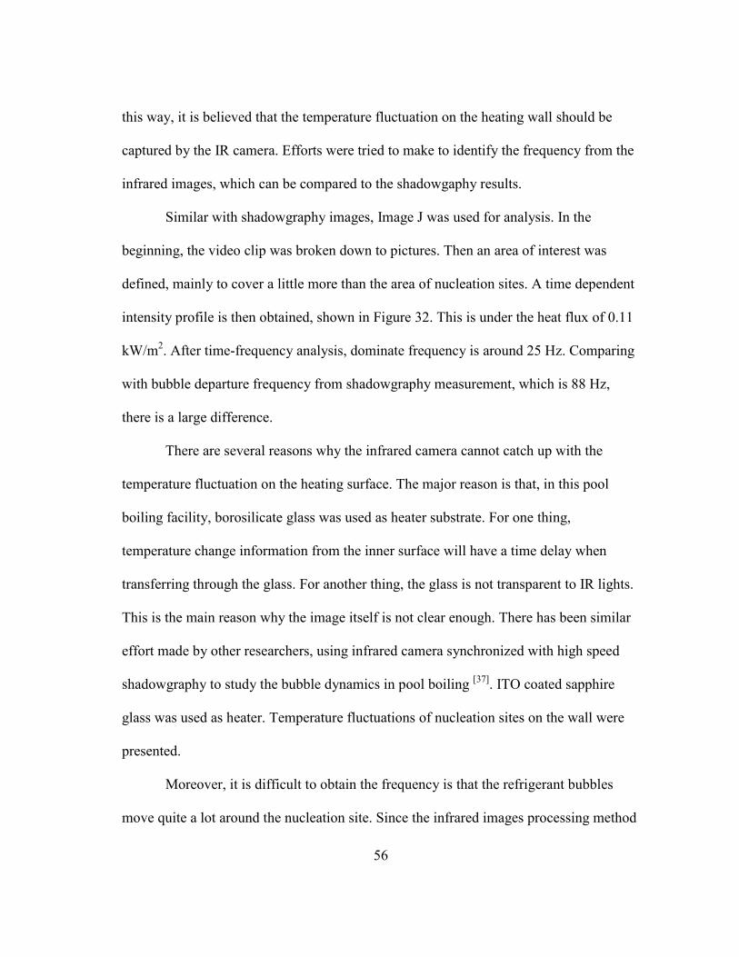
Similar with shadowgraphy images, Image J was used for analysis. In the
beginning, the video clip was broken down to pictures. Then an area of interest was
defined, mainly to cover a little more than the area of nucleation sites. A time dependent
intensity profile is then obtained, shown in Figure 32. This is under the heat flux of 0.11
kW/m2. After time-frequency analysis, dominate frequency is around 25 Hz. Comparing
with bubble departure frequency from shadowgraphy measurement, which is 88 Hz,
there is a large difference.
There are several reasons why the infrared camera cannot catch up with the
temperature fluctuation on the heating surface. The major reason is that, in this pool
boiling facility, borosilicate glass was used as heater substrate. For one thing,
temperature change information from the inner surface will have a time delay when
transferring through the glass. For another thing, the glass is not transparent to IR lights.
This is the main reason why the image itself is not clear enough. There has been similar
effort made by other researchers, using infrared camera synchronized with high speed
shadowgraphy to study the bubble dynamics in pool boiling [37]. ITO coated sapphire
glass was used as heater. Temperature fluctuations of nucleation sites on the wall were
presented.
Moreover, it is difficult to obtain the frequency is that the refrigerant bubbles
move quite a lot around the nucleation site. Since the infrared images processing method
57
is based on the greyscale analysis of the image, the movements of bubbles largely
increase the uncertainty. Different from refrigerant bubbles, water bubbles tend to stick
to the nucleation sites, which makes infrared recording possible. Thus, for future advice,
sapphire glass is preferred for IR thermometry.
Figure 32 Grey scale profile from infrared images
Though the estimation of bubble departure frequency from wall temperature
fluctuations is not successful, the average wall temperature could be estimated through
IR images. Using Image J, the average overheats under three different heat flux are
concluded in the table below. is the measured value from IR images, while is
the actual ITO surface temperature estimated from Equation (16).
218
220
222
224
226
228
230
232
234
0 0.2 0.4 0.6
Gre
y Sc
ale
Time /s
58
Table 2 Wall overheat under different heat flux Current