Graduate Theses and Dissertations Iowa State University Capstones, Theses andDissertations

2017

Experimental studies on the dynamics of in-flightand impacting water droplets pertinent to aircrafticing phenomenaHaixing LiIowa State University

Follow this and additional works at: https://lib.dr.iastate.edu/etd

Part of the Aerospace Engineering Commons

This Dissertation is brought to you for free and open access by the Iowa State University Capstones, Theses and Dissertations at Iowa State UniversityDigital Repository. It has been accepted for inclusion in Graduate Theses and Dissertations by an authorized administrator of Iowa State UniversityDigital Repository. For more information, please contact digirep@iastate.edu.

Recommended CitationLi, Haixing, "Experimental studies on the dynamics of in-flight and impacting water droplets pertinent to aircraft icing phenomena"(2017). Graduate Theses and Dissertations. 15564.https://lib.dr.iastate.edu/etd/15564

Experimental studies on the dynamics of in-flight and impacting water droplets

pertinent to aircraft icing phenomena

by

Haixing Li

A dissertation submitted to the graduate faculty

in partial fulfillment of the requirements for the degree of

DOCTOR OF PHILOSOPHY

Major: Aerospace Engineering

Program of Study Committee:

Hui Hu, Major Professor

Anupam Sharma

Thomas Ward III

Alberto Passalacqua

Xinwei Wang

Iowa State University

Ames, Iowa

2017

Copyright © Haixing Li, 2017. All rights reserved.

ii

DEDICATION

I would like to dedicate this dissertation to my foster mother, Sanying Yao, who just

went to heaven in this June. Since I was in the graduating process, I could not go back

home to accompany her in the last period of her life. Her support is the power for me to

complete this work.

iii

TABLE OF CONTENTS

LIST OF FIGURES ........................................................................................................... vi

LIST OF TABLES ............................................................................................................ xi

ACKNOWLEDGEMENTS .............................................................................................xii

ABSTRACT .................................................................................................................... xiv

CHAPTER 1 GENERAL INTRODUCTION .............................................................. 1

1.1 Background and Motivation ............................................................................... 1

1.2 Thesis Organization .......................................................................................... 11

CHAPTER 2 SIMULTANEOUS MEASUREMENT OF SIZE, FLYING

VELOCITY AND TRANSIENT TEMPERATURE OF IN-FLIGHT DROPLETS

BY USING A MOLECULAR TAGGING TECHNIQUE .............................................. 18

2.1 Introduction ...................................................................................................... 18

2.2 Technical Basis of the Molecular Tagging Technique ..................................... 23

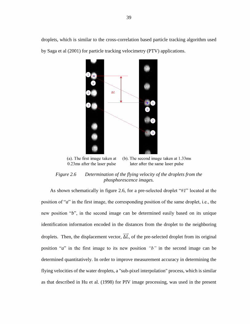
2.3 Measurement Results and Discussions ............................................................ 36

2.4 Conclusions ...................................................................................................... 49

CHAPTER 3 AN EXPERIMENTAL INVESTIGATION ON THE EFFECTS

OF SURFACE HYDROPHOBICITY ON THE ICING PROCESS OF

IMPACTING WATER DROPLETS ............................................................................... 55

3.1 Introduction ...................................................................................................... 55

iv

3.2 Experimental Methods ..................................................................................... 58

3.3 Measurement Results and Discussions ............................................................ 63

3.4 Conclusions ...................................................................................................... 87

CHAPTER 4 QUANTIFICATION OF DYNAMIC WATER DROPLET

IMPACT ONTO A HYDROPHILIC SOLID SURFACE BY USING A DIGITAL

IMAGE PROJECTION TECHNIQUE ............................................................................ 91

4.1 Introduction ...................................................................................................... 91

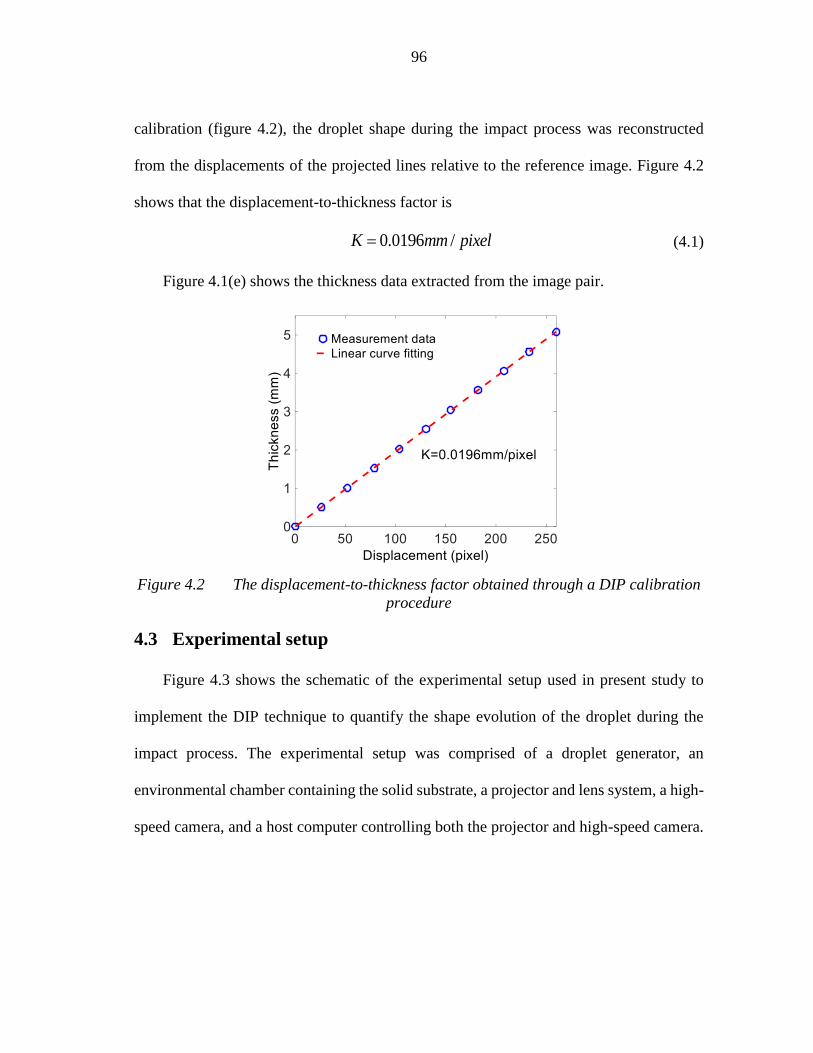
4.2 Water Film / Droplet Thickness Measurements Using DIP Technique ........... 94

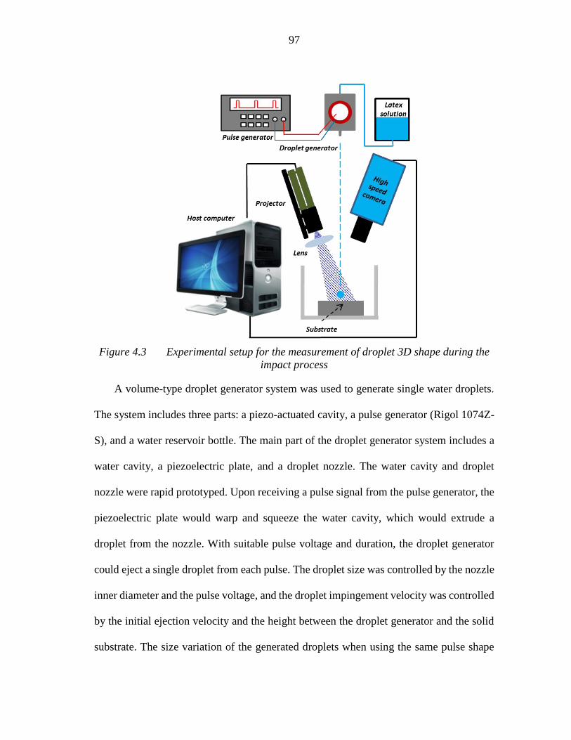
4.3 Experimental setup ........................................................................................... 96

4.4 Results and Discussions ................................................................................... 99

4.5 Conclusions .................................................................................................... 120

CHAPTER 5 MAXIMUM DIAMETER OF IMPACTING LIQUID

DROPLETS ON SOLID SURFACE ............................................................................. 126

5.1 Introduction .................................................................................................... 126

5.2 Experimental Setup ........................................................................................ 129

5.3 Results and Discussions ................................................................................. 135

5.4 Conclusions .................................................................................................... 147

CHAPTER 6 DAMPED HARMONIC SYSTEM MODELING OF DROPLET

OSCILLATING DYNAMICS DURING THE OSCILLATING STAGE ON A

HYDROPHILIC SURFACE .......................................................................................... 153

6.1 Introduction .................................................................................................... 153

v

6.2 Experimental Setup ........................................................................................ 156

6.3 Results and Discussions ................................................................................. 160

6.4 Conclusions .................................................................................................... 170

CHAPTER 7 CONCLUSIONS AND FUTURE WORK ........................................ 174

7.1 Conclusions .................................................................................................... 174

7.2 Future Work ................................................................................................... 181

vi

LIST OF FIGURES

Figure 2.1 Timing chart of lifetime-based MTT technique ····························· 26

Figure 2.2 Absorption and emission spectra of 1-BrNp·Gβ-CD·ROH triplex 34. ··· 31

Figure 2.3 Variation of droplet temperature versus phosphorescence lifetime

(Neopentyl alcohol was used to make 1-BrNpM-CDROH triplex) ··············· 32

Figure 2.4 Experiment Setup Used for the Demonstration Experiments·············· 34

Figure 2.5 Determination of in-flight droplet size from the acquired

phosphorescence images ···································································· 38

Figure 2.6 Determination of the flying velocity of the droplets from the

phosphorescence images. ··································································· 39

Figure 2.7 Simultaneous measurements of droplet size, flying velocity and

transient temperature of the in-flight droplets by using molecular tagging

technique ······················································································ 42

Figure 2.8 The temperature of the in-flight droplets at 100mm away from the

droplet generator as a function of the initial temperature of the water droplets ···· 48

Figure 2.9 The temperature of the in-flight droplets as a function of flying time ··· 49

Figure 3.1 Schematic of the experimental setup for measuring droplet

impingement and ice accretion ····························································· 59

Figure 3.2 Main part of the droplet generator system ···································· 60

Figure 3.3 Schematic of the droplet impingement solid substrate ····················· 62

vii

Figure 3.4 Water droplets on compared surfaces: (a) Hydrophilic surface; (b)

Superhydrophobic surface. ································································· 64

Figure 3.5 Droplet impact process on the normal temperature substrates ············ 68

Figure 3.6 The surface temperature variation of the impact droplet on the

normal temperature substrates ······························································ 71

Figure 3.7 The circumferentially-averaged surface temperature on the normal

temperature surfaces of the impact droplet during cooling process ·················· 71

Figure 3.8 The temperature variation of the central point of the surface of the

impact droplet on hydrophilic and superhydrophobic surface (SHS) ················ 73

Figure 3.9 Droplet impact process on the icing temperature substrates ··············· 75

Figure 3.10 The surface temperature variation of the impact droplet on the icing

temperature substrates ······································································· 79

Figure 3.11 The circumferentially-averaged surface temperature of the impact

droplet during the cooling process ························································· 79

Figure 3.12 Heat transfer directions during the phase change process of icing ······· 80

Figure 3.13 The comparison of the temperature variation processes at the central

point of the droplets impacting on icing temperature hydrophilic and

superhydrophobic substrates (SHS) ······················································· 82

Figure 3.14 The temperature variation of the impact droplet surface central point

on the hydrophilic surfaces under different temperature ······························· 84

Figure 3.15 The temperature variation of the central point on the hydrophilic

surfaces under different temperature and different droplet impact velocity ········· 87

viii

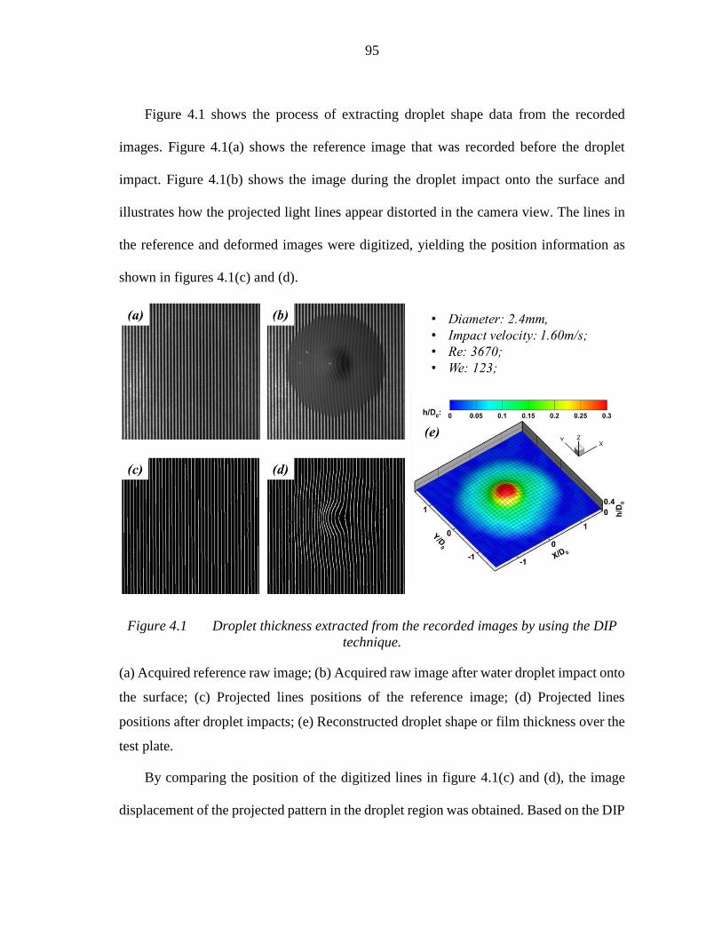
Figure 4.1 Droplet thickness extracted from the recorded images by using the

DIP technique. ················································································ 95

Figure 4.2 The displacement-to-thickness factor obtained through a DIP

calibration procedure ········································································ 96

Figure 4.3 Experimental setup for the measurement of droplet 3D shape during

the impact process············································································ 97

Figure 4.4 Spreading stage of the droplet impact process ····························· 101

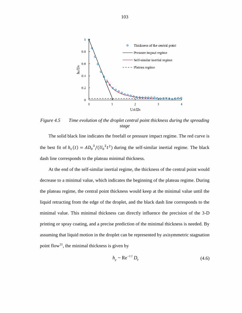
Figure 4.5 Time evolution of the droplet central point thickness during the

spreading stage ············································································· 103

Figure 4.6 Minimal thickness of the plateau ℎ𝑝 as a function of the Reynolds

number Re, and the two suspected laws 𝑅𝑒1/2 and 𝑅𝑒2/5 are shown as a

guide. ···················································································· 105

Figure 4.7 Receding stage of the droplet impact process······························ 107

Figure 4.8 Oscillating stage of the droplet impact process ···························· 109

Figure 4.9 The average thickness along radius of the three distinct moments of

three different impact cases ······························································· 111

Figure 4.10 The impact droplet shape at the end of the spreading stage under

different impact conditions ······························································· 113

Figure 4.11 Time evolution of the droplet central point thickness under different

impact conditions ·········································································· 114

ix

Figure 4.12 Comparison of experimental and the damped harmonic model results

of the time evolution of the droplet central point thickness under different

impact conditions during the oscillating stage. ········································ 118

Figure 4.13 DIP technique measurement accuracy ······································ 120

Figure 5.1 Experimental setup for measurement of the maximum spreading of

the impacting droplet ······································································ 130

Figure 5.2 The surface area factor f as a function of Reynolds number Re,

Weber number We and combination of Re and We as 𝑊𝑒 ∗ 𝑅𝑒1/2. ·············· 140

Figure 5.3 Comparison of the model (based on energy balance) prediction

results with the experimental data ······················································· 143

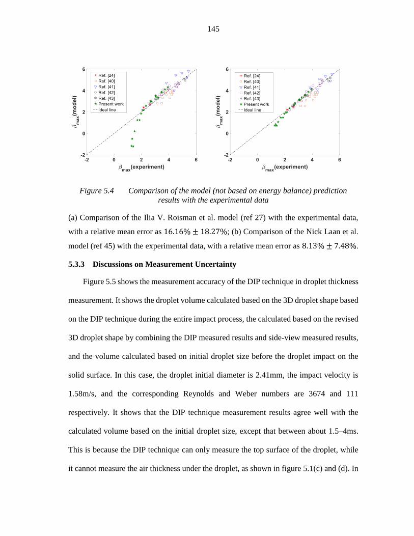
Figure 5.4 Comparison of the model (not based on energy balance) prediction

results with the experimental data ······················································· 145

Figure 5.5 Measurement accuracy of the DIP technique ······························ 147

Figure 6.1 Experimental setup for measurement of the droplet shape variation

during impact process ····································································· 157

Figure 6.2 Comparison of predictions of the damping coefficient 𝛼 and

frequency of the oscillator 𝜔 from equation 6.13a and 6.13b with experimental

data. ···················································································· 164

Figure 6.3 Comparison of predictions of the maximum upper central height

ℎ𝑐𝑚𝑎𝑥/𝐷0 from equation 6.14 with experimental data. ····························· 165

Figure 6.4 Transient variation of flattening factor 𝛿 of droplet on the solid

substrate ···················································································· 168

x

Figure 6.5 Transient variation of flattening factor 𝛿 of droplet on the solid

substrate with different impact velocity ················································ 169

xi

LIST OF TABLES

Table 3.1 Emissivity coefficients of materials used in the measurements ·············· 63

Table 3.2 The measured surface properties of the two impact substrates ··············· 65

Table 3.3 The final receding diameter/area/height of the impingement droplet on

hydrophilic and superhydrophobic surfaces under normal temperature ············· 73

Table 3.4 The final receding diameter/area/height of the impingement droplet on

hydrophilic and superhydrophobic surfaces under icing temperature ················ 81

Table 3.5 The final receding diameter/area/height of the impingement droplet on

hydrophilic surfaces under different temperature ······································· 82

Table 3.6 The final receding diameter/area/height of the impingement droplet on

hydrophilic surfaces under different temperature and different droplet

impingement velocity ······································································· 85

Table 4.1 The initial diameter before droplet impact on the solid surface, the

impact velocity, and corresponding Reynolds and Weber number under three

different conditions ········································································ 110

Table 5.1 The impact conditions of the droplets ·········································· 132

Table 6.1 The impact conditions of the droplets ·········································· 159

xii

ACKNOWLEDGEMENTS

I would like to express my sincere gratitude and appreciation to my major advisors,

Dr. Hui Hu, whose expertise, enthusiasm, and research attitude have been influencing me

during my entire Ph.D. period. Without his generous guidance and support, this

dissertation would not have been possible. I consider it a great honor to work with these

prominent professors in the past four years.

My heartily appreciation also goes to my committee members, Dr. Anupam Sharma,

Dr. Thomas Ward III, Dr. Alberto Passalacqua, and Dr. Xinwei Wang,for their generous

help during my research. I would also like to thank them for evaluating my research work

and giving me many insightful comments.

I am grateful to all the staff members in the Department of Aerospace Engineering,

especially former and present department sectaries, Ms. Gayle Fay and Ms. Jacqueline

Kester for their help on all the paperwork and many other important things.

I would like to thank Dr. Rye Waldman, and Dr. Kai Zhang for their valuable help in

completing the experiments and thesis writing. I also want to thank Dr. Wenwu Zhou, Dr.

Yang Liu, Mr. Morteza Khosravi, Mr. Zhe Ning, Mr. Pavithra Premaratne, Mr. Linkai Li,

Mr. Hao Guo and Mr. Liqun Ma for their help and the joys shared in the past four years.

I am also hugely grateful to my father and mother, Kang Li, and Chunmei Li, who

have given me this opportunity to study abroad. I cannot become who I am without their

unconditional love and support throughout my life.

xiii

Finally, my deepest appreciation is reserved for my fiancee, Yan Cao, who has always

been supporting me during my Ph.D. study. With her love and encouragement, I have been

able to overcome many difficulties in my life.

xiv

ABSTRACT

Aircraft icing is widely recognized as a significant hazard to aircraft operations in

cold weather. When an aircraft or rotorcraft flies in a cold climate, some of the super-

cooled water droplet would impact and freeze on the exposed aircraft surfaces to form ice

shapes, which can degrade the aerodynamic performance of an airplane significantly by

decreasing lift while increasing drag, and even lead to the aircraft crash. In the present

study, a series of experimental investigations were conducted to investigate dynamics and

thermodynamics of in-flight and impinging water droplets in order to elucidate the

underlying physics of the important micro-physical process pertinent to aircraft icing

phenomena.

A novel lifetime-based molecular tagging thermometry technique (MTT) is

developed to achieve simultaneous measurements of droplet size, flying velocity and

transient temperature of in-flight water droplets to characterize the dynamic and

thermodynamic behaviors of the micro-sized in-flight droplets pertinent to aircraft icing

phenomena. By using high-speed imaging and infrared thermal imaging techniques, a

comprehensive experimental study was conducted to quantify the unsteady heat transfer

and phase changing processes as water droplets impinging onto frozen cold surfaces under

different test conditions (i.e., with different Weber numbers, Reynolds numbers, and

impact angles of the impinging droplets, different temperature, hydrophobicity and

roughness of the test plates) to simulate the scenario of super-cooled water droplets

impinging onto the frozen cold wing surfaces. A novel digital image projector (DIP)

xv

technique was also developed to achieve time-resolved film thickness measurements to

quantify the dynamic impinging process of water droplets (i.e., droplet impact, rebounding,

splashing and freezing process). An impact droplet maximum spreading diameter model

and a damped harmonic oscillator model were proposed based on precise measurement of

the impact droplet 3D shape. A better understanding of the important micro-physical

processes pertinent to aircraft icing phenomena would lead to better ice accretion models

for more accurate prediction of ice formation and accretion on aircraft wings as well as to

develop more effective and robust anti-/de-icing strategies for safer and more efficient

operation of aircraft in cold weather.

1

CHAPTER 1

GENERAL INTRODUCTION

1.1 Background and Motivation

Aircraft icing is widely recognized as a significant hazard to aircraft operations in

cold weather. When an aircraft or rotorcraft flies in certain climates, some of the

supercooled droplets in the air would impact and freeze on the exposed aircraft surfaces

and form ice shapes. Ice may accumulate on every exposed frontal surface of an airplane,

not only on the wing, propeller and windshield, but also on the antennas, vents, intakes,

and cowlings. Icing accumulation can degrade the aerodynamic performance of an

airplane significantly by decreasing lift while increasing drag. In moderate to severe

conditions, an airplane could become so iced up that continued flight is impossible. The

airplane may stall at much higher speeds and lower angles of attack than normal. It could

roll or pitch uncontrollably, and recovery may be impossible. Ice can also cause engine

stoppage by either icing up the carburetor or, in the case of a fuel-injected engine, blocking

the engine’s air source. The importance of proper ice control for aircraft operation in cold

climate was highlighted by many aircraft crashes in recent years like the ATR-72 aircraft

of American Eagle flight crashed in Roselawn, Indiana due to ice buildup on its wings

killing all 66 people aboard on October 31, 1994. After investigation, it was found that the

aircraft encountered the supercooled large droplets (SLD) icing environment, which didn’t

be defined in Appendix C of Part 25 of Federal Aviation Regulations (FAR25 Appendix

C), and the aircraft crashed for the abnormal icing on airfoils1. The study of atmosphere

shows that the abnormal icing condition wasn’t defined in the FAR 25 Appendix C2, thus

2

the deicer equipment designed based on the FAR 25 Appendix C is not suitable for the

abnormal icing environment. For expanding the airworthiness regulations application

scope of icing environment, it is important and necessary to elucidate the underlying

physics of the abnormal icing.

As the basis of the aircraft icing phenomenon, the droplet impact and icing is a

complicated process relating to a series fluid dynamic theories and thermodynamics

theories. To elucidate the underlying physics, a series of investigation were desired.

1.1.1 In-flight droplet temperature, velocity and size measurement

The temperature, impact velocity and size of the droplet can severely influence the

droplet impact and icing process, thus, a technique that can simultaneously measure the

droplet temperature, velocity and size before impacting is desired.

It is well known that both fluorescence and phosphorescence are molecular

photoluminescence phenomena. Compared with fluorescence, which typically has a

lifetime on the of order nanoseconds, phosphorescence can last as long as microseconds,

even minutes. Since emission intensity is a function of the temperature for some

substances, both fluorescence and phosphorescence of tracer molecules may be used for

temperature measurements. While fluorescence (LIF) techniques have been widely used

for temperature measurements of liquid droplets in spray flows 3–5, Laser-induced

phosphorescence (LIP) techniques have also been suggested recently to conduct

temperature measurements of ‘‘in-flight” or levitated liquid droplets 6,7. Compared with

LIF-based thermometry techniques, the relatively long lifetime of LIP has been used to

prevent interference from scattered/reflected light and any fluorescence from other

3

substances (such as from solid surfaces for the near surface measurements) that are present

in the measurement area, by simply putting a small time delay between the laser excitation

pulse and the starting time for phosphorescence image acquisitions 8. Furthermore, LIP

was found to be much more sensitive to temperature compared with LIF 6,7, which is

favorable for the accurate temperature measurements of small liquid droplets.

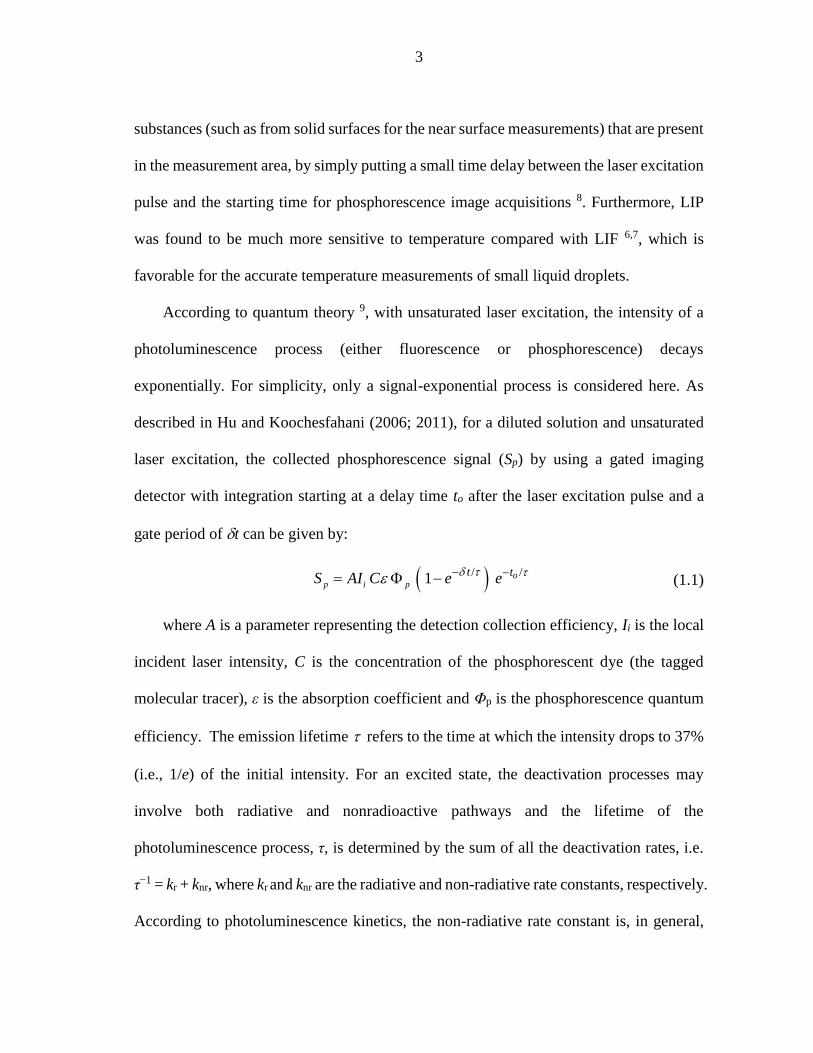
According to quantum theory 9, with unsaturated laser excitation, the intensity of a

photoluminescence process (either fluorescence or phosphorescence) decays

exponentially. For simplicity, only a signal-exponential process is considered here. As

described in Hu and Koochesfahani (2006; 2011), for a diluted solution and unsaturated

laser excitation, the collected phosphorescence signal (Sp) by using a gated imaging

detector with integration starting at a delay time to after the laser excitation pulse and a

gate period of t can be given by:

/ /1p i p

ot tS AI C e e

(1.1)

where A is a parameter representing the detection collection efficiency, Ii is the local

incident laser intensity, C is the concentration of the phosphorescent dye (the tagged

molecular tracer), ε is the absorption coefficient and Φp is the phosphorescence quantum

efficiency. The emission lifetime refers to the time at which the intensity drops to 37%

(i.e., 1/e) of the initial intensity. For an excited state, the deactivation processes may

involve both radiative and nonradioactive pathways and the lifetime of the

photoluminescence process, τ, is determined by the sum of all the deactivation rates, i.e.

τ−1 = kr + knr, where kr and knr are the radiative and non-radiative rate constants, respectively.

According to photoluminescence kinetics, the non-radiative rate constant is, in general,

4

temperature dependent (Ferraudi, 1988), and the resulting temperature dependence of the

phosphorescence lifetime is the basis of the present technique for temperature

measurement.

It should also be noted that the absorption coefficient ε, and quantum yield Φp are

usually temperature dependent in general 12, resulting in a temperature-dependent

phosphorescence signal (Sp). Thus, in principle, the collected phosphorescence signal (Sp)

may be used to measure temperature if the incident laser intensity and the concentration

of the phosphorescent dye remain constant (or are known) in the region of interest.

As shown in Equation (1.1), the collected phosphorescence signal (Sp) is also a

function of the incident laser intensity (Ii) and the concentration of the phosphorescent dye

(C), thus, the spatial and temporal variations of the incident laser intensity and the non-

uniformity of the phosphorescent dye (such as due to photo bleaching and/or the changes

of the dye concentration in liquid droplets during evaporation process) in the region of

interest would have to be corrected separately in order to derive quantitative temperature

data from the acquired phosphorescence images. In practice, however, it is very difficult,

if not impossible, to ensure a non-varying incident laser intensity distribution and a

constant dye concentration within liquid droplets due to evaporation process, which may

cause significant errors in the temperature measurements. To overcome this problem, Hu

and Koochesfahani (2003; 2006; 2011) developed a lifetime-based Molecular Tagging

Thermometry (MTT) technique， which can eliminate the effects of incident laser

intensity and concentration of phosphorescent dye on temperature measurements

effectively.

5

1 2ln( / )

t

S S

(1.2)

Where τ is the phosphorescence lifetime, ∆𝑡 is the time delay of two successive image,

and 𝑆1/𝑆2 is the phosphorescence intensity ratio.

As described in Hu and Koochesfahani (2006, 2011) and Hu et al (2010), since the

photoluminescence lifetime is temperature dependent for some molecular tracers, with the

conditions of diluted solution and unsatuated laser exciation, the temperature distribution

in a fluid flow can be derived from the distribution of the intensity ratio of the two

photoluminescence images acquired after the same laser excitation pulse. For a given

molecular tracer and fixed t value, Equation (1.2) defines a unique relation between

phosphorescence intensity ratio (R) and fluid temperature T, which can be used for

thermometry as long as the temperature dependence of phosphorescence lifetime of the

molecular tracers is known. This ratiometric approach eliminates the effects of any

temporal and spatial variations in the incident laser intensity (due to pulse-to-pulse laser

eneragy variations) and non-uniformity of the dye concentration (e.g., due to

photobleaching or concentration change of the tracer molecules within liquid droplets due

to evaporation at a high temperature environment).

In addition to measuring the transient temperature of liquid droplets, droplet size and

flying velocity of the in-flight droplets can also be determined simultaneously based on

the acquired phosphorescence image pair. With a pre-calibrated scale ratio between the

image plane and the object plane for the phosphorescence image acquisition, the size of

the in-flight droplets can be determined quantitatively by measuring the dimension of the

6

droplets in the acquired phosphorescence images via an image processing procedure.

Furthermore, a particle-tracking algorithm can be used to determine the displacement

vectors of the in-flight droplets between the two phosphorescence image acquisitions.

Since the time delay Δt between the two image acquisition is known for a specific

experiment, the flying velocities of the in-flight droplets can also be estimated based on

the measured displacement vectors of the in-flight droplets between the two

phosphorescence image acquisitions.

The objective of present study is to develop a molecular tagging technique for

achieving simultaneous measurements of droplet size, flying velocity and transient

temperature of in-flight liquid droplets.

1.1.2 Droplet impact and icing

In recent year, the frequently used de-icing systems on aircraft are based on two

techniques, the mechanical technique, as the de-icing boots, and the other one is the

heating technique, as the electrical heater mats. While both of these two ways would

expand the power from aircraft, a passive de-icing technique which can help reduce the

ice accretion on aircraft is desired. The recent researches on superhydrophobic surfaces

demonstrated that the superhydrophobic coatings have ice phobic properties 16, as the

droplets can bounce off of cold superhydrophobic surfaces without freezing 17 and the

superhydrophobicity directly implies anti-icing functionality 18. Therefore, utilizing the

superhydrohopbic surfaces could be a reasonable way to manage the water runback

phenomenon and decrease or eliminate the back-part icing on airfoil. Superhydrophobic

surfaces have been extensively studied because they exhibit a number of interesting

7

properties such as extremely high static contact angles (e.g., >150˚), small contact angle

hysteresis, droplets rolling off at shallow surface angles, and droplets bouncing on impact

19–23. These properties of superhydrophobic surfaces leads to self-cleaning behavior,

whereby water droplets quickly roll off the surface and carry with them any other

contaminates-including other droplets-they encounter. The superhydrophobicity of the

surface results from a combination of chemical hydrophobicity with a micro or nano

textured surface. The structure of the surface plays an important role both in the wettability

of the surface and in the ability of the surface to resist ice accretion 16. Since the

superhydrobic surface demonstrates ice phobic properties, an investigation of the surface’s

influence to droplet impact and icing process is desired.

Droplet impact, such as the fingering of an inkblot or a coffee stain, is familiar to

everyone. Droplet impact, which has been studied extensively since 187624, has a very

wide range of applications, including atomization processes25, raindrop dynamics26, inkjet

printing27, blood pattern and drop trajectories28, and micro-fabrication29. While it also

involves most of the key issues of surface flows, droplet impact is characteristic of

multiphase flows30. In the previous studies, a typical droplet impact process usually

includes an early contact stage that considers the central bubble31 and skating on air32, a

spreading or splash stage33,34, and a receding or rebounding stage35,36. While most of the

previous studies were concentrated on the air layer radius or thickness12,13, maximum

spreading radius35,36,37, minimal thickness of the water layer38, and whether the impacting

droplet would splash34,39 or rebounding35,36, very few studies considered the droplet shape

evolution during the impact process. Since the droplet shape evolution during the impact

8

process can directly influence the final shape of the impact droplet under icing conditions40,

e.g. droplet impact and icing on the airfoil, and then influence the impact surface for the

subsequent droplet, the accurate measurement of the droplet shape or the film thickness

of the impact droplet could help reveal the underlying physics and improve the theoretical

physics models used in the airfoil icing.

The most frequently-used method to measure the droplet shape is using high speed

camera to record the impact process from the side view41,42. When a droplet normally

impacts on a flat surface, it is acceptant to assume that the impact droplet is axially

symmetric, and a 2-D profile can represent the real shape of the droplet. However, if the

impact direction was not perpendicular to the impact surface, or the surface was not flat

enough, then the real droplet shape during the impact process would be much more

complicated, and a 2-D profile cannot represent of the real shape41. Moreover, in some

moments during the droplet impact process, especially during the droplet spreading stage,

the central region of the droplet is lower than the outer region43, and thus the central region

information is blocked by the outer region, which leads to the failure of obtaining droplet

shape information by side view. A method which can record real 3-D shape information

of impact droplet is needed. At present, there are several techniques can collect the

thickness information of objects, e.g., using multi-transducer ultrasonic pulse-echo

technique was used to measure the film flow thickness44, and using space-time-resolved

Fourier transform profilometry technique (FTP) to measure the 3-D shape of objective45,46.

The ultrasonic pulse-echo technique can just do point thickness measurement, while the

FTP technique need several different successive fringe patterns to achieve high accuracy

9

measurement, which leads to the limitation of the time resolution. Since the droplet impact

process, especially the spreading stage is quite fast and needs high time resolution 3-D

shape information to analyze the dynamics during the impact process, a method which can

achieve both thickness measurement of the full droplet and high time resolution is needed.

As a very important parameter during droplet impact process, the maximum spreading

diameter can directly influence the ice collection efficient on the aircraft since it dominates

the ice area of the impact droplet. To predict the maximum spreading diameter of the

impact droplet, a large number of different models have been proposed for the maximum

spreading factor 𝛽𝑚𝑎𝑥. For example, Scheller & Bousfield47 proposed an empirical law

based on experimental results; Pasandideh-Fard et al.48 developed a spreading factor

model based on detailed energy balance between the initial droplet prior impact and the

droplet at the maximum spreading; Ukiwe & Kwok49 extended the above model with an

approximated static contact angle and a cylinder assumption; Clanet et al.50 came up with

a spreading factor scale by considering the mass balance using the impact capillary length;

Roisman51 and Eggers et al.52 raised the spreading factors using dynamical model for the

spreading of the droplet involving a viscous boundary layer. Comparing with those

spreading factor models based on mass balance or using dynamical model, the spreading

factor models based on detailed energy balance give explicit values, while most of the

others give scales and need more conditions and analyses to obtain the explicit values.

However, those spreading factors based on the energy balance need more accurate

experimental data instead of assumptions to improve the prediction accuracy. For example,

Pasandideh-Fard et al.48 assumed that the shape of the droplet at the maximum spreading

10

was a circle, while Ukiwe & Kwok49 assumed it as a cylinder, while the real shape of the

droplet at the maximum spreading was much more complex than just a circle or cylinder,

especially under low Reynolds and Weber numbers impacting conditions. To increase the

prediction accuracy, a method is needed to precisely measure the shape of the impact

droplet at the maximum spreading.

The droplet impact and icing process is a combination of dynamic and

thermodynamic process, thus, a high precise prediction of droplet impact dynamics as the

flatness factor during the oscillating stage of a droplet can help increase the prediction

accuracy of aircraft icing. When predicting the dynamic droplet behavior, the

computational modeling is an attractive means, however, the process is challenging as it

requires accurate tracking and prediction of the continuously deforming gas-liquid

interface. Moreover, the contact line velocity along with impact substrate and liquid

properties has not been universally successful in achieving the level of accuracy that is

needed for simulations. Thus, a simple model that can predict the dynamic behaviors

during oscillating stage is desirable. A few previous studies already proposed some models,

for example, for example, Manglik developed a damped harmonic system model to predict

the dimensionless spread factor 𝛽 (= D/𝐷0) and flatness factor δ (= h/𝐷0), where D and

h are the droplet diameter and the height of upper surface central point of the droplet

during the droplet post-impact process, and 𝐷0 is the initial diameter of the droplet before

impacting. In this damped harmonic system model, the damping coefficient and frequency

of the oscillation were calculated based on semi-empirical models derived from measured

11

experimental results, and the Reynolds number and Weber number as in equation 6.1 and

6.2 were set as the variables in the semi-empirical models.

The objectives of the present study are:

1. Investigate the superhydrophobic surface’s influence to the droplet impact and

icing process;

2. Develop a method to obtain the time resolved 3D shape of impacting droplets

during the whole impact process to quantify the dynamic impacting process of droplets;

3. Propose a droplet maximum spreading diameter model based on energy

conservation during the impact process;

4. Analyze the droplet dynamics during the oscillating stage, and propose a model

that can predict the flatness factor of the droplet during the oscillating stage.

1.2 Thesis Organization

The dissertation includes seven chapters in total. A general introduction (Chapter 1)

is given at the beginning, and the conclusions and future work are provided as the last

chapter of the dissertation (Chapter 7).

Chapter 2 describes the development of the molecular tagging technique, which is

used to be used in the measurements of in-flight droplet temperature, flying velocity and

size. To validate the accuracy of the temperature measurement, the results measured by

the lift time based molecular tagging technique were compared with the predicted results.

Chapter 3 presents an experimental investigation of the droplet impact and icing on

normal (hydrophilic surface) and superhydrophobic surface. A high-speed imaging

12

technique was used to recording the droplet profile variation, while a thermometry

imaging technique was implemented to achieve temporally and spatially resolved

temperature distribution measurements of the droplet during the impact process. The

comparison of the dynamics and temperature of the droplets impacting on these two

surfaces were discussed in detail.

Chapter 4 introduces the development of the digital image projector (DIP) technique

to measure the 3D shape of the impact droplet during the impact process. Based on the

measured results, the droplet impact process can be divided into three distinct stages:

spreading stage, receding stage, and oscillating stage. The measured results helped

validate the models proposed in previous studies. By comparing the droplet shape

evolution under different impact velocities, the dynamics of droplet impact under different

Weber numbers or Reynolds numbers was analyzed in detail.

Chapter 5 described a revised impact droplet maximum spreading diameter model

based on detailed energy conservation during the impact process by precisely measure the

droplet 3D shape. A combination of digital image technique and “side-view” technique

helped precisely measure the 3D shape of the droplet when the droplet reaches the

maximum spreading diameter. To validate the prediction precise, the predicted results

were compared with the experimental data in present study and that in several previous

researches, meanwhile, several prediction models proposed in previous studies were

analyzed as well.

Chapter 6 presented an analysis of the droplet dynamics during the oscillating stage,

and introduce the development of a damped harmonic oscillator model that can predict the

13

flatness factor of the droplet during the oscillating stage. To validate the prediction

accuracy, the predicted results of the model were compared with the experimental results

in the present study.

References

1 Report, A. A., “National Transportation Safety in-Flight Icing Encounter and Loss

of Control,” vol. 1, 1994.

2 Cober, S. G., Isaac, G. A., and Ratvasky, T. P., “Assessment of aircraft icing

conditions observed during AIRS,” AIAA 40th Aerospace Sciences Meeting &

Exhibit, Reno, NE, 2002.

3 Zhang, Y., Zhang, G., Xu, M., and Wang, J., “Droplet temperature measurement

based on 2-color laser-induced exciplex fluorescence,” Experiments in Fluids,

vol. 54, Jul. 2013, p. 1583.

4 Castanet, G., Lavieille, P., Lemoine, F., Lebouché, M., Atthasit, A., Biscos, Y.,

and Lavergne, G., “Energetic budget on an evaporating monodisperse droplet

stream using combined optical methods,” International Journal of Heat and Mass

Transfer, vol. 45, Dec. 2002, pp. 5053–5067.

5 Lavieille, P., Lemoine, F., Lavergne, G., and Lebouché, M., “Evaporating and

combusting droplet temperature measurements using two-color laser-induced

fluorescence,” Experiments in Fluids, vol. 31, Jul. 2001, pp. 45–55.

6 Omrane, A., Juhlin, G., Ossler, F., and Aldén, M., “Temperature measurements of

single droplets by use of laser-induced phosphorescence,” Applied optics, vol. 43,

2004, pp. 3523–3529.

7 Omrane, A., Santesson, S., Alden, M., and Nilsson, S., “Laser techniques in

acoustically levitated micro droplets.,” Lab on a chip, vol. 4, Aug. 2004, pp. 287–

91.

8 Hu, H., and Huang, D., “Simultaneous measurements of droplet size and transient

temperature within surface water droplets,” AIAA journal, vol. 47, 2009, pp. 813–

820.

9 Ramamurthy, V., and Schanze, K. S., Organic and inorganic photochemistry,

1998.

14

10 Hu, H., and Koochesfahani, M. M., “Thermal effects on the wake of a heated

circular cylinder operating in mixed convection regime,” Journal of Fluid

Mechanics, vol. 685, Oct. 2011, pp. 235–270.

11 Hu, H., and Koochesfahani, M. M. M., “Molecular tagging velocimetry and

thermometry and its application to the wake of a heated circular cylinder,”

Measurement Science and Technology, vol. 17, Jun. 2006, pp. 1269–1281.

12 Kim, H. J., Kihm, K. D., and Allen, J. S., “Examination of ratiometric laser

induced fluorescence thermometry for microscale spatial measurement

resolution,” International Journal of Heat and Mass Transfer, vol. 46, Oct. 2003,

pp. 3967–3974.

13 Hu, H., and Koochesfahani, M., A Novel Technique for Quantitative Temperature

Mapping in Liquid by Measuring the Lifetime of Laser Induced Phosphorescence,

2003.

14 Hu, H., and Koochesfahani, M., “Molecular tagging velocimetry and thermometry

and its application to the wake of a heated circular cylinder,” Measurement

Science and Technology, vol. 17, 2006, pp. 1269–1281.

15 Hu, H., Jin, Z., and Nocera, D., “Experimental investigations of micro-scale flow

and heat transfer phenomena by using molecular tagging techniques,”

Measurement Science and Technology, vol. 21, 2010, p. 085401 (14pp).

16 Cao, L., Jones, A. K., Sikka, V. K., Wu, J., and Gao, D., “Anti-Icing

superhydrophobic coatings,” Langmuir, vol. 25, 2009, pp. 12444–12448.

17 Maitra, T., Tiwari, M. K., Antonini, C., Schoch, P., Jung, S., Eberle, P., and

Poulikakos, D., “On the nanoengineering of superhydrophobic and impalement

resistant surface textures below the freezing temperature (Supporting Material),”

Nano Letters, vol. 14, 2014, pp. 172–182.

18 Vorobyev, A. Y., and Guo, C., “Multifunctional surfaces produced by

femtosecond laser pulses,” Journal of Applied Physics, vol. 117, 2015, p. 033103.

19 Antonini, C., Villa, F., and Marengo, M., “Oblique impacts of water drops onto

hydrophobic and superhydrophobic surfaces: outcomes, timing, and rebound

maps,” Experiments in Fluids, vol. 55, 2014, p. 1713.

20 Bartolo, D., Bouamrirene, F., Verneuil, É., Buguin, A., Silberzan, P., and

Moulinet, S., “Bouncing or sticky droplets: Impalement transitions on

superhydrophobic micropatterned surfaces,” Europhysics Letters (EPL), vol. 74,

2006, pp. 299–305.

15

21 Blossey, R., “Self-cleaning surfaces--virtual realities.,” Nature materials, vol. 2,

2003, pp. 301–306.

22 Dorrer, C., and Rühe, J., “Some thoughts on superhydrophobic wetting,” Soft

Matter, vol. 5, 2009, p. 51.

23 Miwa, M., Nakajima, A., Fujishima, A., Hashimoto, K., and Watanabe, T.,

“Effects of the surface roughness on sliding angles of water droplets on

superhydrophobic surfaces,” Langmuir, vol. 16, 2000, pp. 5754–5760.

24 Worthington, “On the forms assumed by drops of liquids falling vertically on a

horizontal plate,” 1876, pp. 261–272.

25 Eggers, J., and Villermaux, E., “Physics of liquid jets,” vol. 71, 2008.

26 Planchon, O., “A Physical Model for the Action of Raindrop Erosion on Soil

Microtopography,” vol. 74, 2010.

27 Minemawari, H., Yamada, T., Matsui, H., Tsutsumi, J., Haas, S., Chiba, R.,

Kumai, R., and Hasegawa, T., “Inkjet printing of single-crystal films,” Nature,

vol. 475, 2011, pp. 364–367.

28 Attinger, D., Moore, C. B., Donaldson, A., and Stone, H. A., “Fluid dynamics

topics in bloodstain pattern analysis : Comparative review and research

opportunities,” 2013.

29 Antkowiak, A., Audoly, B., and Josserand, C., “Instant fabrication and selection

of folded structures using drop impact,” vol. I.

30 Rein, M., “Phenomena of liquid drop impact on solid and liquid surfaces,” vol.

12, 1993, pp. 61–93.

31 Engineering, M., Drive, E., and Engineering, E., “The air bubble entrapped under

a drop impacting on a solid surface,” vol. 545, 2005, pp. 203–212.

32 Street, G., and Street, G., “Air cushioning with a lubrication/inviscid balance,”

vol. 482, 2003, pp. 291–318.

33 Eggers, J., Fontelos, M. A., Josserand, C., Zaleski, S., Eggers, J., Fontelos, M. A.,

Josserand, C., and Zaleski, S., “Drop dynamics after impact on a solid wall :

Theory and simulations Drop dynamics after impact on a solid wall : Theory and

simulations,” vol. 062101, 2016.

34 Chr. Mundo, M. Sommerfeld, C. T., “Droplet-Wall Collisions: Experimental

Studies of the Deformation and Breakup Process,” vol. 21, 1995.

16

35 Rioboo, R., Heat, E., and Sa, P., “Outcomes from a Drop Impact on Solid

Surfaces,” 2001.

36 Statistique, P., and Lhomond, R., “Retraction dynamics of aqueous drops upon

impact on non-wetting surfaces,” vol. 545, 2005, pp. 329–338.

37 Roisman, I. V, Berberović, E., Tropea, C., Roisman, I. V, Berberovi, E., and

Tropea, C., “Inertia dominated drop collisions . I . On the universal flow in the

lamella Inertia dominated drop collisions . I . On the universal flow in the

lamella,” vol. 052103, 2016.

38 Lagubeau, G., Fontelos, M. A., Josserand, C., Maurel, A., Pagneux, V., and

Petitjeans, P., “Spreading dynamics of drop impacts,” 2012, pp. 50–60.

39 Xu, L., Zhang, W. W., and Nagel, S. R., “Drop Splashing on a Dry Smooth

Surface,” vol. 184505, 2005, pp. 1–4.

40 Zhang, C., and Liu, H., “Effect of drop size on the impact thermodynamics for

supercooled large droplet in aircraft icing Effect of drop size on the impact

thermodynamics for supercooled large droplet in aircraft icing,” vol. 062107,

2016.

41 Josserand, C., and Thoroddsen, S. T., “Drop Impact on a Solid Surface,” pp. 365–

393.

42 Bartolo, D., Josserand, C., and Bonn, D., “Singular Jets and Bubbles in Drop

Impact,” vol. 124501, 2006, pp. 1–4.

43 Li, H., Waldman, R. M., and Hu, H., “An Experimental Investigation on Unsteady

Heat Transfer and Transient Icing Process upon Impingement of Water Droplets,”

2016, pp. 1–18.

44 Liu, Y., Chen, W., Bond, L. J., and Hu, H., “An experimental study on the

characteristics of wind-driven surface water film flows by using a multi-

transducer ultrasonic pulse-echo technique An experimental study on the

characteristics of wind-driven surface water film flows by using a multi-

transducer ultrasonic pulse-echo technique,” vol. 012102, 2017.

45 Hu, H., Wang, B., and Zhang, K., “Quantification of transient behavior of wind-

driven surface droplet / rivulet flows using a digital fringe projection technique,”

Journal of Visualization, 2015, pp. 705–718.

46 Dai, J., Li, B., and Zhang, S., “High-quality fringe pattern generation using binary

pattern optimization through symmetry and periodicity,” Optics and Lasers in

Engineering, vol. 52, 2014, pp. 195–200.

17

47 Scheller, B. L., and Bousfield, D. W., “Newtonian Drop Impact with a Solid

Surface,” vol. 41, 1995, pp. 1357–1367.

48 Fard, M. P., Qiao, Y. M., Chandra, S., Mostaghimi, J., Qiao, Y. M., Chandra, S.,

and Mostaghimi, J., “Capillary effects during droplet impact on a solid surface

Capillary effects during droplet impact on a solid surface,” vol. 650, 1996.

49 Ukiwe, C., and Kwok, D. Y., “On the Maximum Spreading Diameter of

Impacting Droplets on Well-Prepared Solid Surfaces,” 2005, pp. 666–673.

50 CLANET, C. S., BE´GUIN, C. D., RICHARD, D., and QU ´ ER ´E, D.,

“Maximal deformation of an impacting drop ´,” vol. 517, 2004, pp. 199–208.

51 Roisman, I. V, and Roisman, I. V, “Inertia dominated drop collisions . II . An

analytical solution of the Navier – Stokes equations for a spreading viscous film

Inertia dominated drop collisions . II . An analytical solution of the Navier –

Stokes equations for a spreading viscous film,” vol. 052104, 2010.

52 Eggers, J., Fontelos, M. A., Josserand, C., and Zaleski, S., “Drop dynamics after

impact on a solid wall : Theory and simulations,” 2010, pp. 1–13.

18

CHAPTER 2

SIMULTANEOUS MEASUREMENT OF SIZE, FLYING VELOCITY AND

TRANSIENT TEMPERATURE OF IN-FLIGHT DROPLETS BY USING A

MOLECULAR TAGGING TECHNIQUE

2.1 Introduction

The characterization of in-flight liquid droplets in spray flows is of great interests for

a wide range of engineering applications, which include combustion, spray cooling, spray

drying, and fire extinction. The heat and mass transfer processes from or to liquid droplets

are important control variables in many of such applications. For examples, the process

of breaking up or atomization of liquid fuel into droplets in the form of a fine spray plays

a pivotal role in improving energy efficiency and suppressing pollutant formation for

various gas turbines and internal combustion (IC) engines. A detailed definition of the

dynamic and thermodynamic behaviors of in-flight fuel droplets is essential for the

optimization of liquid fuel injectors/atomizers in order to maximize energy efficiency,

minimize pollutant emissions, and meet the operability requirements of a particular

application 1. Spray cooling, as an effective technique to remove heat from a hot surface,

has been used widely to control quenching rates in metallurgical industry 2 and to achieve

fast cooling of hot electronics components 3. As reported in4, while the size and initial

temperature of liquid droplets influence the amount of sensible heating that can be

removed in spray cooling, the behavior of the small in-flight liquid droplets would be

affected by the rising hot gas or vapor resulting from the evaporation at the hot surface,

inhibiting any subcooling effect. Thus, the quantitative information to describe the

19

dynamic and thermodynamic characteristics of the small in-flight droplets is indispensable

for the design optimization to augment the heat transfer from the hot surface in spray

cooling applications.

The dynamic and thermodynamic characteristics of in-flight droplets in spray flows

are usually quantified in the terms of droplet size, flying velocity, and temperature of the

droplets. While the size and flying velocity of liquid droplets may affect the heat and mass

transfer processes between the droplets and the surrounding gas flows via convection,

droplet temperature is actually one of the most important properties, which is directly

related to the heat and mass transfer from or to the liquid droplets through atomization

or/and evaporation process. Among various parameters of interest in characterizing the

dynamic and thermodynamic behavior of droplets in spray flows, droplet temperature is

the one of the least investigated due to the lack of suitable non-intrusive measurement

techniques.

Global rainbow thermometry (GRT) technique, which is based on the rainbow

position and its dispersion as a function of the refractive index dependent on temperature,

has been developed to measure the size and temperature of liquid droplets in spray flows5,6.

Since liquid droplets are assumed to be perfectly spherical in GRT, non-spherical droplets

may cause significant systematic errors in GRT measurements 6,7. While Wilms et al.8

proposed an approach to improve GRT technique by filtering out the non-spherical

droplets to reduce biased errors, the inevitable presence of refractive index gradients

induced by the non-uniform temperature distributions within liquid droplets would still

cause significant biased errors in GRT measurements5,6.

20

Laser induced fluorescence (LIF) technique has also been used for temperature

measurement of liquid droplets in spray flows. LIF-based thermometry techniques are

based on the temperature dependence of LIF intensity for some fluorescent tracer

molecules premixed within the liquid droplets. In applying LIF-based thermometry

techniques to measure temperature of liquid droplets, two detecting bands from the

fluorescence spectra (i.e., 2-colors LIF-based thermometry) were usually chosen in order

to minimize the effects of the non-uniformities of the illuminating laser intensity and

fluorescence dye concentration on the temperature measurements 9–11. To implement 2-

color LIF-based thermometry techniques, two cameras with various optical filters are

usually required, along with a very careful image registration or coordinate mapping

procedure in order to get the quantitative spatial relation between the two acquired LIF

images. In addition, other complications also need to be carefully considered, such as the

relatively low temperature sensitivity, the spectral conflicts to cause re-absorption of

fluorescent emission, and photo bleaching of the fluorescence dyes in using 2-color LIF-

based thermometry approaches for the temperature measurements of in-flight droplets

9,11,12.

While several other measurement techniques, which include Raman scattering13–15,

thermochromics liquid crystal thermometry16–18 and infrared imaging thermography19,20,

have also been used to measure the temperatures of liquid droplets, almost of them have

relatively poor measurement accuracy and require complicated experimental setup to

achieve quantitative temperature measurements of small in-flight liquid droplets. More

recently, Lemoine & Castanet21 provide a comprehensive review of various optical

21

techniques for quantitative measurements of temperature and chemical composition of

droplets.

Simultaneous measurements of droplet size, flying velocity, and transient temperature

of in-flight droplets are highly desirable to characterize the dynamic and thermodynamic

behaviors of liquid droplets in spray flows. While some of the measurement techniques

described above can measure the droplet size and temperature of the liquid droplets in

spray flows, none of those techniques can provide quantities measurements of the flying

velocity of the in-flight droplets simultaneously. Those techniques are required to combine

with other velocimetry techniques such as laser Doppler velocimetry (LDV) or particle

imaging velocimetry (PIV) in order to achieve simultaneous measurements of droplet size,

flying velocity and temperature of the liquid droplets in spray flows, which would

complicate the experimental setup and add extra burdens on the instrumentation cost for

the measurements.

In the present study, we report the progress made in our recent efforts to develop a

novel molecular tagging technique for simultaneous measurements of droplet size, flying

velocity and transient temperature of liquid droplets in spray flows. The molecular tagging

technique described here is a Laser Induced phosphorescence (LIP) based technique,

which can be considered an extension of the molecular tagging velocimetry and

thermometry technique developed by Hu & Koochesfahani22. For the molecular tagging

measurements, a pulsed laser is used to “tag” phosphorescent tracer molecules premixed

within liquid droplets (i.e., water droplets for the present study). The long-lived LIP

emission is imaged at two successive times after the same laser excitation pulse. The size

22

of the liquid droplets is determined quantitatively based on the acquired droplet images

with a pre-calibrated scale ratio between the image plane and the object plane. A particle-

tracking algorithm is used to determine the displacement vectors of the in-flight droplets

between the two LIP image acquisitions, thereby, to estimate the flying velocities of the

liquid droplets. The transient temperature of the in-flight droplets is derived by taking

advantage of the temperature dependence of the phosphorescence lifetime, which is

estimated from the phosphorescence intensity ratio of the droplets in the two interrogations.

It should be noted that, while molecular tagging techniques have been developed and

successfully applied to achieve flow velocity and temperature measurements in single-

phase flows23,24 and stationary surface droplets25,26, the work presented here will deal with

a multiphase spray flow system involving in-flight liquid droplets with transient

temperature change and unsteady heat transfer with ambient gas phase flows. The work

described here, to our knowledge, is the first of its nature that is capable of achieving

simultaneous measurements of droplet size, flying velocity and transient temperature of

in-flight liquid droplets in spray flows. No similar work has ever been published/reported

before. It can be implemented with only a single intensified CCD camera, a single-pulsed

Ultraviolet (UV) laser and phosphorescent molecules for the simultaneous measurements

of multiple important properties in spray flows, which offers significant advantages over

other flow diagnostic techniques to characterize spray flows.

In the following sections, the technical basis of a lifetime-based molecular tagging

thermometry (MTT) technique for the transient temperature measurements of in-flight

droplets is described briefly at first. Then, the related physical properties of the

23

phosphorescent 1-BrNpM-CDROH triplex for the molecular tagging measurements is

introduced. The feasibility and implementation of the molecular tagging technique are

demonstrated by conducting simultaneous measurements of droplet size, flying velocity

and transient temperature of micro-sized water droplets exhausted from a piezoelectric

droplet generator into ambient air at different test conditions in order to characterize the

dynamic and thermodynamic behaviors of the micro-sized in-flight droplets. The

unsteady heat transfer process between the in-flight droplets and the ambient air is also

analyzed theoretically by using the Lumped Capacitance method to predict the dynamic

temperature changes of the in-flight water droplets along their flight trajectories. The

measured temperature data are compared with the theoretical analysis results

quantitatively to validate the measurement results.

2.2 Technical Basis of the Molecular Tagging Technique

2.2.1 Technical basis of molecular tagging technique for droplet temperature

measurement

It is well known that both fluorescence and phosphorescence are molecular

photoluminescence phenomena. Compared with fluorescence, which typically has a

lifetime on the of order nanoseconds, phosphorescence can last as long as microseconds,

even minutes. Since emission intensity is a function of the temperature for some

substances, both fluorescence and phosphorescence of tracer molecules may be used for

temperature measurements. While fluorescence (LIF) techniques have been widely used

for temperature measurements of liquid droplets in spray flows 9–11, Laser-induced

phosphorescence (LIP) techniques have also been suggested recently to conduct

24

temperature measurements of ‘‘in-flight” or levitated liquid droplets 27,28. Compared with

LIF-based thermometry techniques, the relatively long lifetime of LIP has been used to

prevent interference from scattered/reflected light and any fluorescence from other

substances (such as from solid surfaces for the near surface measurements) that are present

in the measurement area, by simply putting a small time delay between the laser excitation

pulse and the starting time for phosphorescence image acquisitions 25. Furthermore, LIP

was found to be much more sensitive to temperature compared with LIF 27,28, which is

favorable for the accurate temperature measurements of small liquid droplets. The

molecular tagging technique described here is a LIP based technique.

According to quantum theory 29, with unsaturated laser excitation, the intensity of a

photoluminescence process (either fluorescence or phosphorescence) decays

exponentially. For simplicity, only a signal-exponential process is considered here. As

described in Hu and Koochesfahani22,24, for a diluted solution and unsaturated laser

excitation, the collected phosphorescence signal (Sp) by using a gated imaging detector

with integration starting at a delay time to after the laser excitation pulse and a gate period

of t can be given by:

/ /1p i p

ot tS AI C e e

(2.1)

where A is a parameter representing the detection collection efficiency, Ii is the local

incident laser intensity, C is the concentration of the phosphorescent dye (the tagged

molecular tracer), ε is the absorption coefficient and Φp is the phosphorescence quantum

efficiency. The emission lifetime refers to the time at which the intensity drops to 37%

(i.e., 1/e) of the initial intensity. For an excited state, the deactivation processes may

25

involve both radiative and nonradioactive pathways and the lifetime of the

photoluminescence process, τ, is determined by the sum of all the deactivation rates, i.e.

τ−1 = kr + knr, where kr and knr are the radiative and non-radiative rate constants, respectively.

According to photoluminescence kinetics, the non-radiative rate constant is, in general,

temperature dependent (Ferraudi, 1988), and the resulting temperature dependence of the

phosphorescence lifetime is the basis of the present technique for temperature

measurement.

It should also be noted that the absorption coefficient ε, and quantum yield Φp are

usually temperature dependent in general 30, resulting in a temperature-dependent

phosphorescence signal (Sp). Thus, in principle, the collected phosphorescence signal (Sp)

may be used to measure temperature if the incident laser intensity and the concentration

of the phosphorescent dye remain constant (or are known) in the region of interest.

As shown in Equation (2.1), the collected phosphorescence signal (Sp) is also a

function of the incident laser intensity (Ii) and the concentration of the phosphorescent dye

(C), thus, the spatial and temporal variations of the incident laser intensity and the non-

uniformity of the phosphorescent dye (such as due to photo bleaching and/or the changes

of the dye concentration in liquid droplets during evaporation process) in the region of

interest would have to be corrected separately in order to derive quantitative temperature

data from the acquired phosphorescence images. In practice, however, it is very difficult,

if not impossible, to ensure a non-varying incident laser intensity distribution and a

constant dye concentration within liquid droplets due to evaporation process, which may

cause significant errors in the temperature measurements. To overcome this problem, Hu

26

and Koochesfahani22,24,31 developed a lifetime-based Molecular Tagging Thermometry

(MTT) technique， which can eliminate the effects of incident laser intensity and

concentration of phosphorescent dye on temperature measurements effectively.

Figure 2.1 Timing chart of lifetime-based MTT technique

The lifetime-based MTT technique works as follows: As illustrated in figure 2.1, a

pulsed laser is used to “tag” phosphorescent tracer molecules premixed within working

liquids (i.e., water for the present study). LIP emission is interrogated at two successive

times after the same laser excitation pulse. The first image is detected at the time ott

after laser excitation for a gate period t to accumulate the phosphorescence intensity 1S ,

while the second image is detected at the time ttt o for the same gate period to

accumulate the phosphorescence intensity 2S . As described in Hu & Koochesfahani22,24,31,

by taking integration of Equation (2.1) on the temporal window Δt, the accumulated

phosphorescence intensities 1S and 2S can determined, and the ratio of the two

phosphorescence signals (R) can be expressed as:

27

2 1

)/ ( /

/

/ /

1/

1

i p

i p

to

o

t t

t

t t

AI C e eR S S e

AI C e e

(2.2)

It indcates that the intensity ratio of the two successive phosphorescence images (R)

is only a funtion of the phosphorescence lifetime and the time delay Δt between the

two image acqusitions, which is a controllable parameter. Based on Equation (2.2), the

phosphorescence lifetime of the molecular tracers can be calculated according to

1 2ln( / )

t

S S

(2.3)

As described in Hu and Koochesfahani (2006, 2011) and Hu et al (2010), since the

photoluminescence lifetime is temperature dependent for some molecular tracers, with the

conditions of diluted solution and unsatuated laser exciation, the temperature distribution

in a fluid flow can be derived from the distribution of the intensity ratio of the two

photoluminescence images acquired after the same laser excitation pulse. For a given

molecular tracer and fixed t value, Equation (2.2) defines a unique relation between

phosphorescence intensity ratio (R) and fluid temperature T, which can be used for

thermometry as long as the temperature dependence of phosphorescence lifetime of the

molecular tracers is known. This ratiometric approach eliminates the effects of any

temporal and spatial variations in the incident laser intensity (due to pulse-to-pulse laser

eneragy variations) and non-uniformity of the dye concentration (e.g., due to

photobleaching or concentration change of the tracer molecules within liquid droplets due

to evaporation at a high temperature environment).

28

To implement the lifetime-based MTT technique described above, only one laser

pulse is required to excite or ‘tag’ the tracer molecules for each instantaneous temperature

measurement. The two successive acquisitions of the photoluminescence image of the

tagged tracer molecules can be achieved using a dual-frame intensified CCD camera.

Compared to the two-color LIF thermometry techniques described above 9–11, which

usually require two CCD cameras with proper optical filters to acquire two fluorescent

images simultaneously for each instantaneous temperature measurement, the present

lifetime-based MTT technique is much easier to implement and can significantly reduce

the burden on the instrumentation and experimental setup. Furthermore, since LIF

emission is short lived with the emission lifetime on the order of nanoseconds, LIF images

are usually acquired when the incident laser illumination is still on; therefore, they are

vulnerable to the contaminations of scattered/reflected light and any fluorescence emission

from other substances. For the lifetime-based MTT technique describe here, as

schematically indicated in figure 2.1, the small time delay between the illumination laser

pulse and the phosphorescence image acquisition can effectively eliminate all the effects

of scattered/reflected light and any fluorescence from other substances that are present in

the measurement region. Since only the phosphorescence emission of the tagged

phosphorescent molecules was acquired for the MTT measurements, the acquired

phosphorescence images of the water droplet are quite “clean”, in comparison with LIF

images.

29

2.2.2 Simultaneous measurements of droplet size and flying velocity of in-flight

droplets

In addition to measuring the transient temperature of liquid droplets, droplet size and

flying velocity of the in-flight droplets can also be determined simultaneously based on

the acquired phosphorescence image pair. With a pre-calibrated scale ratio between the

image plane and the object plane for the phosphorescence image acquisition, the size of

the in-flight droplets can be determined quantitatively by measuring the dimension of the

droplets in the acquired phosphorescence images via an image processing procedure.

Furthermore, a particle-tracking algorithm can be used to determine the displacement

vectors of the in-flight droplets between the two phosphorescence image acquisitions.

Since the time delay Δt between the two image acquisition is known for a specific

experiment, the flying velocities of the in-flight droplets can also be estimated based on

the measured displacement vectors of the in-flight droplets between the two

phosphorescence image acquisitions.

Further technical details about the simultaneous quantification of droplet size and

flying velocity, in addition to the transient temperature measurements, of the in-flight

droplets, will be described in the “Results and Discussions” section of the present study.

2.2.3 Phosphorescence molecular tracer used in the present study

It is well known that laser-induced phosphorescence techniques usually surfer from

oxygen quenching to phosphorescence emission. In the present study, a specially designed

phosphorescent triplex (1-BrNpM-CDROH) was used as the molecular tracer for the

molecular tagging measurements. The phosphorescent 1-BrNpM-CDROH triplex is

actually the mixture compound of three different chemicals, which are lumophore

30

(indicated collectively by 1-BrNp), maltose--cyclodextrin (indicated collectively by M-

CD) and alcohols (indicated collectively by ROH). According to Hartmann et al (1996)

and Gendrich et al (1997), the special molecular structures of the phosphorescent triplex

(1-BrNpM-CDROH) would form a molecular shell to prevent laser-induced

phosphorescence emission of the excited 1-BrNp molecules from oxygen quenching

effects.

Figure 2.2(a) shows the normalized absorption and emission spectra of the

phosphorescent 1-BrNpM-CDROH triplex. The fluorescence and phosphorescence

spectra are both shown in the plot, and the phosphorescence emission is significantly red-

shifted relative to fluorescence. It should be noted that, because of the large red shift as

shown in the figure, there is no overlap between the phosphorescence emission and

absorption spectra, which suggests that the phosphorescence does not get re-absorbed with

the phosphorescent triplex (1-BrNpM-CDROH) as the molecular tracer for flow

measurements. Figure 2.2(b) shows the emission spectra of the 1-BrNpM-CDROH

solution at different temperatures. As shown clearly in the figure, while the

phosphorescence emission of the triplex is very temperature sensitive, its fluorescence is

almost independent of temperature. The fluorescence lifetime of 1-BrNpM-CDROH

triplex is within 20 ns, while its phosphorescence lifetime is found to be much longer, on

the order of several milliseconds, as reported in Hu et al (2006) and Hu & Koochesfahani

(2006, 2011). Further information about the chemical and photoluminescence properties

of the phosphorescent triplex (1-BrNpM-CDROH) is available at Hartmann et al (1996)

and Gendrich et al (1997).

31

Figure 2.2 Absorption and emission spectra of 1-BrNp·Gβ-CD·ROH triplex 34.

(a) Normalized absorption & emission spectra. (b) Emission spectra at different temperatures.

Upon the pulsed excitation of a UV laser (i.e., quadrupled wavelength of Nd:YAG

laser at 266nm for the present study), the phosphorescence lifetime of the phosphorescent

triplex (1-BrNpM-CDROH) molecules in an aqueous solution was found to change

significantly with temperature. Figure 2.3 shows the measured phosphorescence lifetimes

of the 1-BrNpM-CDROH molecules as a function of temperature, which were obtained

through a calibration experiment similar as those described in Hu & Koochesfahani (2006).

It can be seen clearly that phosphorescence lifetime of 1-BrNpM-CDROH molecules

varies greatly with increasing temperature, decreasing from about 2.7 ms to 1.9 ms as the

temperature changes from 10.0oC to 20.0oC. The relative temperature sensitivity of the

phosphorescence lifetime is about 3.3% per degree Celsius, which is much higher than

those of fluorescent dyes used for LIF-based thermometry measurements. For comparison,

the temperature sensitivity of Rhodamine B widely used for LIF-based thermometry is

less than 2.0% per degree Celsius12,34.

32

Figure 2.3 Variation of droplet temperature versus phosphorescence lifetime

(Neopentyl alcohol was used to make 1-BrNpM-CDROH triplex)

In the present study, we used a concentration of 2104 M for M-CD, a saturated

(approximately 1105 M) solution of 1-BrNp, and a concentration of 0.03M for

Neopentyl alcohol (ROH) in making 1-BrNpM-CDROH triplex. It should be noted

that, while Cyclohexanol alcohol was widely used to make 1-BrNpM-CDROH triplex

for molecular tagging measurements in the previous studies 24,31,34,35, Neopentyl alcohol

used in the present study was found to increase the phosphorescence intensity of the 1-

BrNpM-CDROH triplex significantly. However, the phosphorescence lifetime of 1-

BrNpM-CDROH triplex was found to become much shorter when the Neopentyl

alcohol was used in making 1-BrNpM-CDROH triplex. For example, at the room

temperature of T=20C, the phosphorescence lifetime of 1-BrNpM-CDROH triplex

with Cyclohexanol alcohol would be about 3.7ms as reported in Hu et al. (2010). However,

1.6

1.8

2.0

2.2

2.4

2.6

2.8

8 10 12 14 16 18 20

Curve fittingMeasurement data

Temperature (C)

Ph

osp

ho

resc

ence

lif

etim

e (m

s)

33

it becomes only about 1.9 ms when Neopentyl alcohol was used to make 1-BrNpM-

CDROH triplex, as shown in figure 2.3.

2.2.4 Experimental setup for demonstration experiments

Figure 2.4 shows the schematic of the experimental setup used in the present study to

demonstrate the feasibility and implementation of the molecular tagging technique

described above to achieve simultaneous measurements of droplet size, flying velocity

and transient temperature of in-flight droplets. Water is used as the working fluid in the

present study, and phosphorescent triplex (1-BrNpM-CDROH) was premixed with

water in a reservoir tank. As shown schematically in figure 2.4, a high-pressure gas

cylinder was used to press the water inside the reservoir tank flow into a pipeline

connected to a piezoelectric droplet generator. By applying square-wave-shaped signals

to drive the piezoelectric actuator inside the droplet generator, water droplets would be

generated and exhausted from the droplet generator into ambient air in a mono-sized water

droplet stream. By changing the nozzle diameter of the piezoelectric droplet generator,

the diameter of the water droplets exhausted from the droplet generator was adjustable in

the range of 200 μm to 1000 μm (i.e., ~450 μm in diameter for the test cases of the present

study). The velocity of the micro-sized water droplets exhausted from the droplet

generator ranged from 0.1 m/s to 10 m/s by varying the gas pressure applied to the water

reservoir tank. During the experiments, while the temperature of the ambient air was

maintained at a constant room temperature of T = 22 ˚C, the temperature of the water

(i.e., along with 1-BrNpM-CDROH triplex) inside the reservoir tank, monitored by

using a thermocouple, was kept constant at a pre-selected low temperature level (i.e.,

34

ranged from 3˚C to 15˚C) by using a Constant Temperature Bath Circulator. As a result,

the temperature of the water droplets out of the droplet generator was lower than the

ambient air temperature, and the micro-sized droplets in the water droplet stream would

be convectively heated up while flying in the ambient air. Thus, the temperature of the in-

flight water droplets would increase monotonically along their flying trajectories.

Figure 2.4 Experiment Setup Used for the Demonstration Experiments

In the present study, a pulsed Nd:YAG laser at a quadrupled wavelength of 266 nm

(5ns pulse duration) was used to excite or ‘tag’ the molecules of 1-BrNpM-CDROH

triplex within the water droplets. A set of optical lenses and mirrors were used to shape

the laser beam into a laser sheet of ~ 500 m in thickness to illuminate the mono-sized

droplet stream along the central plane of the droplet generator exit. A dual-fame intensified

35

CCD camera (PCO DICAM-Pro, Cooke Corporation, 1280 pixels ×1024 pixels in

resolution) with a fast-decay phosphor (P46) was used to acquire the phosphorescence

images at two successive times after the same laser excitation pulse, as shown

schematically in figure 2.1. For the molecular tagging measurement results given in the

present study, the first phosphorescence image of the in-flight droplets was acquired at

230s after the laser excitation pulse with an exposure time of 100s. The second

phosphorescence image was acquired at 1.1ms later after the same laser pulse with the

same exposure time (i.e., Δt=1.1ms between the image pair). The laser and the camera

were synchronized using a digital delay generator (SRS-DDG535), which controlled the

timing of the laser sheet illumination and the intensified camera data acquisition.

It is also noted that since a low concentration of the phosphorescent 1-BrNpM-

CDROH triplex was used for the present study, the effects of the molecular tracers on the

physical properties of water are believed to be small and are assumed to be negligible.

During the experiments, the energy level of the pulse laser used to tag the molecular tracers

within water droplets was below 0.5 mJ/pulse. The repetition rate of the pulsed laser

excitation was set to be 1 Hz. The energy deposited by the excitation laser into the water

droplets was very small, and the temperature rise of the water droplets due to the energy

deposition of the laser excitation was estimated to be very small and is also assumed to be

negligible.

36

2.3 Measurement Results and Discussions

2.3.1 Determination of droplet size from the acquired phosphorescence images

As shown schematically in figure 2.1, to implement the molecular tagging technique

described above, a pulsed laser was used to “tag” 1-BrNpM-CDROH triplex molecules

premixed within the water droplets, and the “tagged” phosphorescent molecules were

imaged at two successive times within the phosphorescence lifetime of the tagged tracer

molecules. Figure 2.5 shows a typical acquired phosphorescence image pair (i.e., the first

phosphorescence image was acquired at 0.23 ms after the laser excitation pulse and the

second phosphorescence image at 1.33 ms after the same laser pulse with the same

exposure time of 0.1 ms) for the molecular tagging measurements. It can been seen that,

since the time delay (i.e., 0.23ms for the present study) between the laser excitation pulse

and the phosphorescence image acquisition can eliminate the scattered/reflected light from

the droplet surfaces and any fluorescence from other substances (e.g., the transparent side

walls of the test rig) near the measurement region effectively, the phosphorescence images

of the water droplets are quite ‘‘clean” even though no optical filter was used in the present

study for the phosphorescence image acquisition.

To implement the molecular tagging technique described above, the image size of the

droplets should be consistent with the physical scale to be solved. Similar as LIF-based

technique, the dynamic range of the droplet size (i.e., the range from the smallest droplet

to the largest droplet) to be measured accurately is limited by the resolution of the digital

camera used for the phosphorescence image acquisition. While the upper limit of the

droplet size (i.e., the largest droplet to be measured accurately using molecular tagging

37

technique) is set by the total pixel number of the digital camera, the lower limit of the

droplet size (i.e., the smallest droplet to be measured accurately) is set by a single pixel of

the digital camera (i.e., the largest water droplets with its image size being only 1 pixel in

the acquired phosphorescence image.

Based on the acquired phosphorescence images as those shown in figure 2.5, the sizes

of the water droplets can be measured quantitatively. Since the phosphorescence, images

of the in-flight droplets are ‘‘clean”, the outer boundaries of the water droplets can be

identified easily in the acquired phosphorescence images by using Matlab-based image

processing software developed “in house”. As shown schematically in figure 2.5(a), a

typical threshold intensity value of 250 for the acquired 12-bit phosphorescence images

was selected in order to determine the outer boundary of a randomly selected water droplet

in the droplet stream, and the diameter of the water droplet was found to be 60 pixels, i.e.,

𝐷0 = 60 pixels, in the acquired phosphorescence images. In the present study, a

parametric study was conducted by using different threshold intensity values (i.e., the

threshold intensity value was changed from 150 to 350) in identifying the outer boundaries

of water droplets in the acquired 12-bit phosphorescence images. The standard deviation

of the measured droplet size in the mono-sized droplet stream was found to be about 2.3

pixels, which is about 4% of the droplet size.

With the pre-calibrated scale ratio between the image plane and the object plane as

given in figure 2.5(b), the size of the randomly selected droplet can be determined

quantitatively, which was measured to be about 450µm.

38

Figure 2.5 Determination of in-flight droplet size from the acquired

phosphorescence images

2.3.2 Determination of flying velocity of the in-flight water droplets

By twisting the square-wave shaped signals supplied to the piezoelectric actuator

inside the droplet generator, the distance between the neighboring droplets in the droplet

stream exhausted from the droplet generator can be manipulated. The information was

used to identify the displacements of any pre-selected droplets in the mono-sized water

droplet stream between the acquired phosphorescence image pair, thereby, the flying

velocity of the droplets can be determined quantitatively from the acquired

phosphorescence image pair. As described above, once the outer boundaries of the

droplets were determined for droplet size measurements, the center locations of the in-

flight droplets in the acquired phosphorescence images as shown in figure 2.6 can be easily

identified by using the Matlab-based image processing software developed “in-house”.

The correspondence of the water droplets in the acquired phosphorescence image pair can

be determined based on the information encoded in the distances among the neighboring

39

droplets, which is similar to the cross-correlation based particle tracking algorithm used

by Saga et al (2001) for particle tracking velocimetry (PTV) applications.

Figure 2.6 Determination of the flying velocity of the droplets from the

phosphorescence images.

As shown schematically in figure 2.6, for a pre-selected droplet “#1” located at the

position of “a” in the first image, the corresponding position of the same droplet, i.e., the

new position “b”, in the second image can be determined easily based on its unique

identification information encoded in the distances from the droplet to the neighboring

droplets. Then, the displacement vector, ∆𝐿 , of the pre-selected droplet from its original

position “a” in the first image to its new position “b” in the second image can be

determined quantitatively. In order to improve measurement accuracy in determining the

flying velocities of the water droplets, a "sub-pixel interpolation" process, which is similar

as that described in Hu et al. (1998) for PIV image processing, was used in the present

40

study to locate the centers of the flying droplets at a sub-pixel level. Based on the statics

of the measured flying velocity of the water droplets in the droplet stream, the standard

deviation of the measured flying velocity of the mono-sized water droplets was found to

be about 3.2 pixels, which is about 1.1% of the displacement of the water droplets between

the acquired phosphorescence image pair (i.e., averaged displacement of the water

droplets given in figure 2.6 is 295.5 pixels. With the time delay between the acquired

phosphorescence image pair known as ∆𝑡 =1.1ms and the pre-calibrated scale ratio

between the image plane and the object plane as that in figure 2.5(b), the flying velocity

of the water droplet “#1” can be calculated as 𝑉 = ∆𝐿 /∆𝑡 For example, for the test case

shown in figure 2.6, the flying velocity of the pre-selected droplet “#1” was measured as

V= 2.03 m/s.

2.3.3 Determination of the transient temperature of the in-flight droplets

After the corresponding positions of the in-flight droplets in the acquired

phosphorescence image pair are determined, the intensity ratio of the same droplets in the

two phosphorescence images can be used to calculate the phosphorescence lifetime of the

1-BrNpM-CDROH triplex molecules within the water droplets by using Equation (2.3).

With the calibration profile of the phosphorescence lifetime vs. temperature as that shown

in figure 2.3, the instantaneous temperature of the in-flight water droplet can be derived

quantitatively from the acquired phosphorescence image pair. For the image processing

of the lifetime-based MTT technique to calculate intensity ratio of the acquired

phosphorescence pair (i.e., S1/ S2), selecting the interrogation windows in the 1st and 2nd

phosphorescence images will be consistent with the scales of the water droplets to be

41

measured. As shown theoretically in Equation (2.3), since the intensity ratio of the

acquired phosphorescence pair, thereby, the lifetime of the phosphorescence emission, is

only the function of the temperature of the tagged phosphorescent tracer molecules, the

dynamic size change of the in-flight droplets due to evaporation would have no effect on

the intensity ratio of the acquired phosphorescence pair. Figure 2.7 gives the

phosphorescence intensity distributions of typical acquired phosphorescence images of

the droplet stream (the black marks/circles on the images indicate the centers of the flying

water droplets) along with the instantaneous temperature of the in-flight droplets derived

from the phosphorescence image pair. As shown in figure 2.7, the instantaneous

temperatures of the in-flight droplets in the center of the measurement window was found

to be 11.9°C, 12.6°C and 11.6°C, respectively.

Based on the time sequence of the measured instantaneous temperature distributions

of the water droplets as those shown in figure 2.7, the dynamic and thermodynamics

characteristics of the in-flight water droplets along their flying trajectories can be revealed

quantitatively, which will be discussed in detail in the following sections.

42

Figure 2.7 Simultaneous measurements of droplet size, flying velocity and transient

temperature of the in-flight droplets by using molecular tagging technique

2.3.4 Theoretical analysis on the unsteady heat transfer process between the in-

flight droplets and ambient air

As described above, since the initial temperature of the water droplets out of the

droplet generator was set to be lower than the temperature of ambient air, the small water

droplets will be convectively heated up while they fly through the ambient air. A

theoretical analysis was performed in the present study by using the Lumped Capacitance

Method to examine the unsteady heat transfer process between the in-flight water droplets

and the ambient air to predict the temperature variations of the in-flight droplets along

their flying trajectories.

The following assumptions are made in the theoretical analysis to examine the

unsteady heat transfer process between the in-flight water droplets and the ambient air:

43

1. The water droplets are assumed to keep their spherical shape while flying in the

ambient air.

2. Negligible radiation effects due to the relatively low temperature of the water

droplets.

3. Negligible small thermal resistance at the droplet surface, and negligible small

temperature change of ambient air around the in-flight water droplet.

4. Since only the spatially-averaged temperature of the water droplets is considered in the

present study and the Biot number of the tiny water droplets (i.e., ~450µm in diameter)

considered here is very small (i.e., Bi = h.D/K<<0.1), the in-flight water droplets are

considered as isothermal spheres with the temperature differences within the micro-sized

water droplets being neglected.

By using the Lumped Capacitance Method described in the heat transfer textbook of

Incropera and Dewitt (2002), the balance of the heat transfer in and out of a control volume

around an in-flight water droplet can be expressed as:

( )s p

dThA T T Vol C

dt (2.4)

Where h is the convection coefficient of air around the surface of the in-flight water

droplet; sA is the surface area of the spherical droplet; T is the transient temperature of

the in-flight droplet to be determined; T is the temperature of ambient air, which is a

constant for the present study; 𝜌 is the density of the water droplet, 𝐶𝑝 is the specific heat

of the droplet; Vol is the volume of the droplet; and t is the time after the water droplet

leaves the droplet generator.

44

Introducing the temperature difference: TT , and recognizing that dt

d

dt

dT ,

Equation (2.4) can be re-written as:

p

s

Vol C d

hA dt

(2.5)

Separating the variables and integrating from the intial condition, for which at 0t

and iTT , it can be derived that

I

tp

os

Vol C ddt

hA

(2.6)

Where TTii .

Evaluating the integral, it can be expresed as

ln( )p i

s

Vol Ct

hA

(2.7)

or

])(exp[ tCVol

hA

TT

TT

p

s

ii

(2.8)

Since 3

6

1DVol and 2DAs for the present study, it can be derived that

)6

exp(/)]6

exp([pp

iDC

th

DC

thTTTT

(2.9)

where D is the diameter of the water droplet.

The convection coefficient h is defined by

D

kh Nu

D (2.10)

45

Where, 𝑁𝑢𝐷 is the Nusselt number, and 𝑘 is the thermal conductivity of air.

As described in Whitaker (1972), the Nusselt number 𝑁𝑢𝐷 around a sphere in air can

be expressed as

1/2 2/3 0.4 1/42 (0.4 Re 0.06 Re ) Pr ( )D D D

s

Nu

(2.11)

Where 𝑅𝑒𝐷 is the Reynolds number of the flying droplet in air, 𝑃𝑟 is the Prandtl

number, 𝜇 is the dynamic viscosity of air at 𝑇𝑖, and 𝑢𝑠 is the mean dynamic viscosity of

air during the droplet heating process.

The Reynold number 𝑅𝑒𝐷 is defined as

ReD

VD

(2.12)

Where, V is the flying velocity of the water droplet, and is the kinematic viscosity

of air.

Based on the Equations (2.9) to (2.12) given above, the transient temperature of the

in-flight water droplets along their flying trajectories can be predicted theoretically with

the known droplet diameter D, flying velocity V, droplet initial temperature 𝑇𝑖 and ambient

air temperature T .

2.3.5 Comparison of measurement results with the theoretical predictions

In the present study, a set of experiments were conducted to examine the unsteady

heat transfer process between the in-flight water droplets and the ambient air at different

test conditions. The molecular tagging technique described above was used to achieve

simultaneous measurements of droplet size, velocity and temperature of the in-flight

droplets. The measured temperature data was compared with the theoretical analysis

46

results quantitatively to validate the measurement results. The measured temperature data

was compared with the theoretical analysis results quantitatively to characterize the

dynamic and thermodynamic behaviors of the in-flight droplets.

Since the experiment is designed mainly to demonstrate the implemented procedure

of the molecular tagging technique, a relatively small temperature range (i.e., between

10°C and 20°C) was chosen for the experiment in order to simplify the experimental setup.

During the experiments, while the ambient air temperature was kept constant at T =

22°C, the initial temperature of the water droplet exhausted from the droplet generator exit

was adjusted from iT =11°C to 18°C. The micro-sized water droplets were convectively

heated up after they were exhausted from the droplet generator into the ambient air. The

measurement window was set to locate at about 100mm away from the exit of the droplet

generator. As shown in figure 2.5 to figure 2.7, the diameter of the water droplets

exhausted from the droplet generator was measured to be about 450 μm with the flying

velocity at about 2.03 m/s. It should be noted that the methodology of the molecular

tagging technique is rather general, and applicable for a much wider temperature range,

depending on the molecular tracers and solutions used for the molecular tagging

measurements ( e.g., 0 ~ 100oC for the phosphorescent triplex (1-BrNpM-CDROH)

premixed in the water droplets). I think we need to do something to improve our ability to

increase the working of the anti-water surface.

Based on 50 frames of the instantaneous measurements as those shown in figure 2.7,

the average temperature of the micro-sized in-flight water droplet at the center of the

measurement window was calculated. Figure 2.8 shows the measured temperature of the

47

in-flight water droplets at 100mm away from the droplet generator as a function of the

initial temperature of the water droplets. The error bars given in the plot represent the

standard deviation values based on the 50 frames of instantaneous temperature

measurements at each test conditions. The predicted temperature values of the in-flight

droplets at different test conditions were also given in the same plot for quantitative

comparison. The predicted temperature values were obtained based on the theoretical

analysis procedure described above (i.e., in section 3.3) with the measured droplet size

(i.e., 450μm in diameter), droplet flying velocity (i.e., V=2.03m/s in flying velocity) and

the initial temperature of the water droplets measured at the exit of the droplet generator

(i.e., iT =11°C to 18°C) as the input parameters. As shown in figure 2.8, the measured

temperatures of the in-flight droplets were found to agree well in general with the

theoretically predicted values. The differences between the measured droplet temperatures

and the predicted values were found to be within 0.5˚C, which is comparable to the

standard derivation values (i.e., indicated as the error bars in the plot) of the instantaneous

temperature measurements.

48

Figure 2.8 The temperature of the in-flight droplets at 100mm away from the droplet

generator as a function of the initial temperature of the water droplets

In the present study, the temperature variations of the in-flight water droplets as a

function of the flying distance in ambient air were also investigated by moving the

measurement window further away from the exit of the droplet generator. During the

experiments, the ambient air temperature was kept constant at T =22 °C, and the initial

temperature of the water droplet exhausted from the droplet generator exit was set at iT

=11°C. Figure 2.9 shows the measured temperatures of in-flight water droplets at different

time after exhausted from the exit of the droplet generator in comparison with the

theoretical predictions. As expected, the temperature of the in-flight water droplets was

found to increase monotonically with the increasing flying time in the ambient air due to

the convective heat transfer between the in-flight water droplets and the ambient air.

While the measured temperature data and the predicted results show a similar tendency as

the flying time increases, the rate of increase of the measured temperature data was found

10

12

14

16

18

20

10 12 14 16 18 20

Theoretic predictionMeasurement data

Initial temperature of the water droplets (C)

Ter

mp

erat

ure

of

the

in-f

lig

ht

dro

ple

ts

at

10

0m

m d

ow

nst

ream

(C

)

49

to be slightly higher than that of the theoretical predictions. As a result, the differences

between the measured temperature data and the predicted results were found to increase

gradually as the flying time increases. The maximum difference between the measured

temperature data and the predicted results was found to be about 1.0˚C with the micro-

sized water droplets flying about 0.2s after exhausted from the exit of the droplet generator.

It should be noted that, in addition to the measurement uncertainty, the simplified theoretic

model that neglects the thermal gradients within the water droplets can also contribute the

differences between the theoretic predictions and the measurement results.

Figure 2.9 The temperature of the in-flight droplets as a function of flying time

2.4 Conclusions

We presented the progress made in developing a molecular tagging technique for

achieving simultaneous measurements of droplet size, flying velocity and transient

temperature of in-flight liquid droplets. Phosphorescent 1-BrNpM-CDROH triplex

5

10

15

20

0 0.05 0.10 0.15 0.20

Theoretical predition

Measurement data

Flying time of the water droplets (s)

Tem

per

atu

re o

f th

e in

-fli

gh

t d

rop

lets

(C

)

50

molecules, which can be turned into long-lasting glowing marks upon excitation by

photons of appropriate wavelength, were used as the molecular tracers for the quantitative

measurements. A pulsed UV laser was used to ‘tag’ the phosphorescent triplex molecules

premixed within in-flight droplets to emit long-lived laser-induced phosphorescence (LIP).

After the same laser excitation pulse, the tagged phosphorescent triplex molecules were

imaged at two successive times within the phosphorescent lifetime of the tracer molecules.

While the size of the in-flight droplets was determined quantitatively based on the

acquired droplet images with a pre-calibrated scale ratio between the image plane and the

object plane, the displacements of the droplets between the two image acquisitions were

used to estimate the flying velocity of the in-flight droplets. The transient temperature of

the in-flight droplets was derived simultaneously by taking advantage of the temperature

dependence of the phosphorescence lifetime, which is estimated from the

phosphorescence intensity ratio of the two interrogations.

The feasibility and implementation of the molecular tagging technique was

demonstrated by conducting simultaneous measurements of droplet size, flying velocity

and transient temperature of micro-sized water droplets exhausted from a piezoelectric

droplet generator at different test conditions. During the experiments, while the ambient

air temperature was kept constant at 22°C, the initial temperature of the micro-sized water

droplet at the droplet generator exit was set at a lower temperature range from 11°C to

18°C. After injected into the ambient air, the micro-sized water droplets were convectively

heated up as they flew through the ambient air, which caused the transient temperature of

the micro-sized water droplets to vary dynamically along their flight trajectories. The

51

unsteady heat transfer process between the in-flight water droplets and the ambient air

were also analyzed theoretically by using the Lumped Capacitance method to predict the

temperature of the in-flight water droplets along their flight trajectories. The measured

temperature data was compared quantitatively with the theoretical analysis results, and the

discrepancies between the measured temperature data and the theoretical prediction results

were found to be within 0.80˚C.

References

1 Schulz, C., and Sick, V., “Tracer-LIF diagnostics: quantitative measurement of

fuel concentration, temperature and fuel/air ratio in practical combustion

systems,” Progress in Energy and Combustion Science, vol. 31, Jan. 2005, pp.

75–121.

2 Hall, D. D., and Mudawar, I., “Experimental and numerical study of quenching

complex-shaped metallic alloys with multiple, overlapping sprays,” International

Journal of Heat and Mass Transfer, vol. 38, May 1995, pp. 1201–1216.

3 Salazar, V. M., Gonzalez, J. E., and Rivera, L. A., “Measurement of Temperatures

on In-Flight Water Droplets by Laser Induced Fluorescence Thermometry,”

Journal of Heat Transfer, vol. 126, Apr. 2004, p. 279.

4 Gonzalez, J. E., and Black, W. Z., “Study of Droplet Sprays Prior to Impact on a

Heated Horizontal Surface,” Journal of Heat Transfer, vol. 119, May 1997, p.

279.

5 van Beeck, J. P., and Riethmuller, M. L., “Nonintrusive measurements of

temperature and size of single falling raindrops.,” Applied optics, vol. 34, 1995,

pp. 1633–1639.

6 van Beeck, J. P., Giannoulis, D., Zimmer, L., and Riethmuller, M. L., “Global

rainbow thermometry for droplet-temperature measurement.,” Optics letters, vol.

24, 1999, pp. 1696–1698.

7 Vetrano, M. R., Gauthier, S., van Beeck, J., Boulet, P., and Buchlin, J.-M.,

“Characterization of a non-isothermal water spray by global rainbow

thermometry,” Experiments in Fluids, vol. 40, Sep. 2005, pp. 15–22.

52

8 Wilms, J., Gréhan, G., and Lavergne, G., “Global Rainbow Refractometry with a

Selective Imaging Method,” Particle & Particle Systems Characterization, vol.

25, Apr. 2008, pp. 39–48.

9 Zhang, Y., Zhang, G., Xu, M., and Wang, J., “Droplet temperature measurement

based on 2-color laser-induced exciplex fluorescence,” Experiments in Fluids,

vol. 54, Jul. 2013, p. 1583.

10 Castanet, G., Lavieille, P., Lemoine, F., Lebouché, M., Atthasit, A., Biscos, Y.,

and Lavergne, G., “Energetic budget on an evaporating monodisperse droplet

stream using combined optical methods,” International Journal of Heat and Mass

Transfer, vol. 45, Dec. 2002, pp. 5053–5067.

11 Lavieille, P., Lemoine, F., Lavergne, G., and Lebouché, M., “Evaporating and

combusting droplet temperature measurements using two-color laser-induced

fluorescence,” Experiments in Fluids, vol. 31, Jul. 2001, pp. 45–55.

12 Coppeta, J., and Rogers, C., “Dual emission laser induced fluorescence for direct

planar scalar behavior measurements,” Experiments in Fluids, vol. 25, Jun. 1998,

pp. 1–15.

13 Schweiger, G., “Raman scattering on single aerosol particles and on flowing

aerosols: a review,” Journal of Aerosol Science, vol. 21, 1990, pp. 483–509.

14 Müller, T., Grünefeld, G., and Beushausen, V., “Rapid communication High-

precision measurement of the temperature of methanol and ethanol droplets using

spontaneous Raman scattering,” vol. 158, 2000, pp. 155–158.

15 Hopkins, R. J., Symes, R., Sayer, R. M., and Reid, J. P., “Determination of the

size and composition of multicomponent ethanol/water droplets by cavity-

enhanced Raman scattering,” Chemical Physics Letters, vol. 380, 2003, pp. 665–

672.

16 Nozaki, T., Mochizuki, T., Kaji, N., and Mori, Y. H., “Application of liquid-

crystal thermometry to drop temperature measurements,” Experiments in Fluids,

vol. 18, 1995, pp. 137–144.

17 Richards, C. D., Richards, R. F., and Boltzman, S., “Transient temperature

measurements in a convectively cooled droplet,” vol. 25, 1998.

18 Mochizuki, T., Nozaki, T., Mori, Y. H., and Kaji, N., “Heat transfer to liquid

drops passing through an immiscible liquid medium between tilted parallel-plate

electrodes,” International Journal of Heat and Mass Transfer, vol. 42, 1999, pp.

3113–3129.

53

19 Tuckermann, R., Bauerecker, S., and Cammenga, H. K., “IR-Thermography of

Evaporating Acoustically Levitated Drops,” International Journal of

Thermophysics, vol. 26, Sep. 2005, pp. 1583–1594.

20 Wulsten, E., and Lee, G., “Surface temperature of acoustically levitated water

microdroplets measured using infra-red thermography,” Chemical Engineering

Science, vol. 63, 2008, pp. 5420–5424.

21 Lemoine, F., and Castanet, G., “Temperature and chemical composition of

droplets by optical measurement techniques : a state-of-the-art review,” 2013.

22 Hu, H., and Koochesfahani, M. M. M., “Molecular tagging velocimetry and

thermometry and its application to the wake of a heated circular cylinder,”

Measurement Science and Technology, vol. 17, Jun. 2006, pp. 1269–1281.

23 Gendrich, C., Koochesfahani, M., and Nocera, D., “Molecular tagging

velocimetry and other novel applications of a new phosphorescent

supramolecule,” Experiments in fluids, vol. 23, 1997, pp. 361–372.

24 Hu, H., and Koochesfahani, M. M., “Thermal effects on the wake of a heated

circular cylinder operating in mixed convection regime,” Journal of Fluid

Mechanics, vol. 685, Oct. 2011, pp. 235–270.

25 Hu, H., and Huang, D., “Simultaneous measurements of droplet size and transient

temperature within surface water droplets,” AIAA journal, vol. 47, 2009, pp. 813–

820.

26 Hu, H., Jin, Z., and Nocera, D., “Experimental investigations of micro-scale flow

and heat transfer phenomena by using molecular tagging techniques,”

Measurement Science and Technology, vol. 21, 2010, p. 085401 (14pp).

27 Omrane, A., Juhlin, G., Ossler, F., and Aldén, M., “Temperature measurements of

single droplets by use of laser-induced phosphorescence,” Applied optics, vol. 43,

2004, pp. 3523–3529.

28 Omrane, A., Santesson, S., Alden, M., and Nilsson, S., “Laser techniques in

acoustically levitated micro droplets.,” Lab on a chip, vol. 4, Aug. 2004, pp. 287–

91.

29 Ramamurthy, V., and Schanze, K. S., Organic and inorganic photochemistry,

1998.

54

30 Kim, H. J., Kihm, K. D., and Allen, J. S., “Examination of ratiometric laser

induced fluorescence thermometry for microscale spatial measurement

resolution,” International Journal of Heat and Mass Transfer, vol. 46, Oct. 2003,

pp. 3967–3974.

31 Hu, H., and Koochesfahani, M., A Novel Technique for Quantitative Temperature

Mapping in Liquid by Measuring the Lifetime of Laser Induced Phosphorescence,

2003.

32 Hu, H., and Koochesfahani, M., “Molecular tagging velocimetry and thermometry

and its application to the wake of a heated circular cylinder,” Measurement

Science and Technology, vol. 17, 2006, pp. 1269–1281.

33 Hartmann, W., Gray, M., and Ponce, A., “Substrate induced phosphorescence

from cyclodextrin· lumophore host-guest complexes,” Inorganica Chimica Acta,

vol. 234, 1996, pp. 239–248.

34 Hu, H., Koochesfahani, M., and Lum, C., “Molecular tagging thermometry with

adjustable temperature sensitivity,” Experiments in fluids, vol. 40, 2006, pp. 753–

763.

35 Hu, H., and Jin, Z., “An icing physics study by using lifetime-based molecular

tagging thermometry technique,” International Journal of Multiphase Flow, vol.

36, 2010, pp. 672–681.

36 Saga, T., Kobayashi, T., Segawa, S., and Hu, H., “Development and evaluation of

an improved correlation based PTV method,” Journal of Visualization, vol. 4,

Mar. 2001, pp. 29–37.

37 Incropera, F., and Dewitt, D., “Introduction to heat transfer, 1996,” John WHey &

Sons. New York. NY.

38 Whitaker, S., “Forced convection heat transfer correlations for flow in pipes, past

flat plates, single cylinders, single spheres, and for flow in packed beds and tube

bundles,” AIChE Journal, vol. 18, Mar. 1972, pp. 361–371.

55

CHAPTER 3

AN EXPERIMENTAL INVESTIGATION ON THE EFFECTS OF SURFACE

HYDROPHOBICITY ON THE ICING PROCESS OF IMPACTING WATER

DROPLETS

3.1 Introduction

Aircraft icing is widely recognized as a significant hazard to aircraft operations in cold

weather. When an aircraft or rotorcraft flies in certain climates, some of the supercooled

droplets in the air would impact and freeze on the exposed aircraft surfaces and form ice

shapes. Ice may accumulate on every exposed frontal surface (under some conditions, the

ice even accumulate at the back part of the airfoil) of an airplane, not only on the wing,

propeller and windshield, but also on the antennas, vents, intakes, and cowlings. Icing

accumulation can degrade the aerodynamic performance of an airplane significantly by

decreasing lift while increasing drag. In moderate to severe conditions, an airplane could

become so iced up that continued flight is impossible. The airplane may stall at much

higher speeds and lower angles of attack than normal. It could roll or pitch uncontrollably,

and recovery may be impossible. Ice can also cause engine stoppage by either icing up the

carburetor or, in the case of a fuel-injected engine, blocking the engine’s air source. The

importance of proper ice control for aircraft operation in cold climate was highlighted by

many aircraft crashes in recent years like the ATR-72 aircraft of American Eagle flight

crashed in Roselawn, Indiana due to ice buildup on its wings killing all 66 people aboard

on October 31, 1994. After investigation, it was found that the aircraft encountered the

supercooled large droplets (SLD) icing environment, which didn’t be defined in Appendix

56

C of Part 25 of Federal Aviation Regulations (FAR25 Appendix C), and the aircraft

crashed for the abnormal icing on airfoils1. The study of atmosphere shows that the

diameter of droplet in the SLD icing environment could vary from 40μm to 1000μm, and

it is far beyond 40μm that defined in FAR252. The deicer equipment designed based on

the FAR 25 Appendix C is not suitable for the SLD icing environment. For expanding the

airworthiness regulations application scope of icing environment, it is important and

necessary to elucidate the underlying physics of SLD icing.

The recent researches on superhydrophobic surfaces demonstrated that the

superhydrophobic coatings have ice phobic properties3, as the droplets can bounce off of

cold superhydrophobic surfaces without freezing4 and the superhydrophobicity directly

implies anti-icing functionality5. Therefore, utilizing the superh ydrohopbic surfaces could

be a reasonable way to manage the water runback phenomenon and decrease or eliminate

the back-part icing on airfoil. Superhydrophobic surfaces have been extensively studied

because they exhibit a number of interesting properties such as extremely high static

contact angles (e.g., >150˚), small contact angle hysteresis, droplets rolling off at shallow

surface angles, and droplets bouncing on impact6–10. These properties of superhydrophobic

surfaces leads to self-cleaning behavior, whereby water droplets quickly roll off the surface

and carry with them any other contaminates-including other droplets-they encounter. The

superhydrophobicity of the surface results from a combination of chemical hydrophobicity

with a micro or nano textured surface. The structure of the surface plays an important role

both in the wettability of the surface and in the ability of the surface to resist ice accretion3.

57

Current ice prediction tools for airfoil icing like LEWICE and FENS AP-ICE make

use of simple classical models that ignore many details of the important micro-physical

processes that responsible of the icing formation and accretion on airfoil11,12. Developing

the technology for safe operation in SLD icing condition requires a better understanding

of the important micro-physical phenomena pertinent to SLD icing. Several studies have

been carried out recently to simulate ice accretion on airfoil icing through icing wind tunnel

testing or calculations. NASA Glenn icing research tunnel analyzed the ice sharp profiles

in different icing conditions by measuring the ice accretion on NACA 0012 airfoil13. Iowa

State icing wind tunnel researched the ice accretion process, the heat transfer process, and

the surface water transport process over an icing accreting NACA 0012 airfoil14,15,16.

Wright and Potapczuk simulate ice accretion on airfoil thought calculation17 by importing

droplet impinging tentative mass model18. Very few studies could be found in literature to

elucidate the underlying physics of SLD icing. The fundamental studies of SLD icing

process could provide detailed information to analyze ice formation and ice-growth

physical processed such as SLD dynamics, unsteady heat transfer process within

supercooled water or ice crystals, which are highly desirable in elucidate the underlying

physics associated with the micro-physical processes.

In the present study, an experimental investigation was conducted to quantify the

unsteady heat transfer and phase change process of icing while droplet impinging onto

different kinds of icing plate as hydrophilic and hydrophobic substrates in order to

elucidate underlying physics to improve our understanding of the important micro-physics

processes pertinent to SLD icing on aircraft wings. The high speed imaging technique was

58

implemented to record the dynamic phase changing process while the infrared

thermometry imaging technique was implemented to achieve temporally-and-spatially

resolved temperature distribution measurements to reveal the time evolution of the

unsteady heat transfer within SLD in the course of icing. A better understanding of the

important micro-physical processes would enable us to improve current icing accretion

models for more accurate prediction of ice formation and ice accretion on aircraft wings

and to develop effective and robust anti-/de-icing strategies to ensure safer and more

efficient operation of aircraft in cold weather.

3.2 Experimental Methods

3.2.1 Experimental setup

Figure 3.1 shows the schematic of the experimental setup used in present study to

implement the high speed imaging technique and infrared thermometry imaging technique

to quantify unsteady heat transfer and phase change process during droplet impact process

to elucidate underlying physics of micro-physical process of droplet impact and icing

phenomena.

The experimental setup was comprised of several subsystems, a droplet generator

system, a droplet impact substrate system, a high speed imaging system, an infrared

imaging system.

59

Figure 3.1 Schematic of the experimental setup for measuring droplet impingement

and ice accretion

3.2.2 Droplet generator system

A volume type of droplet generator system was used to generate the mono water

droplet needed in the experiment. The system includes three parts – main part, pulse

generator, and water supplement bottle. As shown in figure 3.2, the main part of the droplet

generator system was combined by a water cavity, a piezoelectric plate and a nozzle. The

water cavity and nozzle were made by 3-D printer. The water cavity was covered by the

piezoelectric plate, and connected with the water supplement bottle with a water tube.

During experiment, the water upper surface in the bottle was controlled at a level which is

Host computer

Pulse generatorDroplet generator

LED

DI water

Infrared camera

Substrate

Infrared window

Light scattering glass

Glass

Laser

Photodiode

Bias circuit and signal conditioning amplifier

Digital delay generator

Scope

Water bath

60

a little higher than the nozzle of the generator to ensure that the water cavity was full of

water, while the water was not outflow from nozzle due to the capillary effect of the nozzle.

After receiving signal from the pulse generator, the piezoelectric plate would warp and

squeeze the water cavity, and then the droplet was ejected from the nozzle. With suitable

pulse voltage and frequency, the droplet generator can eject only one droplet with one

single pulse. The droplet size was controlled by the nozzle inner diameter and the pulse

voltage while the droplet impact velocity was controlled by the initial ejective velocity

when droplet leaving the nozzle and the perpendicular distance between the droplet

generator and the solid impact substrate. The droplet size can vary from about 0.5mm to

2.5mm by using different inner diameter nozzles and different pulse voltages, while the

impact velocity of the droplet can vary from about 1m/s to 5m/s. To avoid the impurities’,

disturb to the impact and icing process, the water used in the experiment was deionized

water.

Figure 3.2 Main part of the droplet generator system

3.2.3 Droplet impact substrate system

The droplet impact substrate system was combined by an impact substrate and a

cooling plate. As shown in figure 3.3, the cooling plate was connected with a water bath

Piezoelectric plate

Water cavity

Nozzle

Squeeze water cavity

61

(NESLAB RTE-211). by two tubes covered by heat adiabatic layer. With the help of the

cyclic coolant, the cooling plate temperature was controlled by the water bath. The impact

substrate was set on the cooling plate and connected each other by thermally conductive

silicone, so that the substrate surface temperature can also be controlled, and the

temperature was controlled precisely from -8˚C to 20˚C.

Condensation can effectively change the wettability of a solid surface19,20. In order to

avoid condensation on the solid substrate and to control the substrate temperature more

precisely, the substrate was mounted in a relatively closed experimental cell, as shown in

figure 3.1. A light scattering glass was mounted at the rear part of the experimental cell, a

high transmitting glass was mounted at the front part of the cell, and an infrared window

was mounted at the top part of the cell. The only opening of the experimental cell was used

for the entry of the in-flight droplet.

Since the impact substrate was connected with the cooling plate by thermally

conductive silicone, it is easy to change the substrate surface properties by using different

substrates. Both of the hydrophilic and superhydrophobic surfaces were used for

investigation of droplet impact and icing. The hydrophilic surface was coated in a wet-

sanded Rustoleum finished with a static water contact angle of 65˚. The superhydrophobic

surface was given the Hydrobead (Hydrobead.com) superhydrophobic treatment, and the

static contact angle is about 157˚.

62

Figure 3.3 Schematic of the droplet impingement solid substrate

3.2.4 High speed imaging system

The high speed imaging system was combined by a high speed camera and a laser

detecting system. As shown in figure 3.1, a high-speed camera (PCO tech dimax HS) with

a micro lens (Nikon Nikkor 60mm 2.8/D) was configured parallel to the surface of the

solid substrate. Diffuse backlighting was provided by a 20W LED spotlight and the light

scattering glass at the rear part of the experimental cell. The laser detecting system includes

five parts – a laser, a photodiode, a bias circuit and signal conditioning amplifier, a digital

storage oscilloscope (Rigol 1074Z), and a digital delay generator. When a droplet was

released from the droplet generator, it crossed the diode laser beam, disrupting the signal

to the photodiode whose signal was amplified and read out by the digital storage

oscilloscope. The trigger from the oscilloscope initialed the digital delay generator that

controlled timing and exposure of the high-speed camera. The frame rate was set as 10000

fps while the image resolution is 624 by 608 pixels.

3.2.5 Infrared imaging system

A FLIR A600 serious infrared camera was used to measure the droplet temperature

variation during the droplet impact and icing process. The frame rate was set as 200 fps

SubstrateThermally

conductive silicone

Coolant in Coolant out

Cooling plate

63

while the image resolution is 640 by 120 pixels. The infrared camera was mounted above

the solid substrate at a distance of 200mm, and the infrared radiation from the substrate

surface and water/ice can be transmitted through the infrared window with a transmission

coefficient of 0.82. The emissivity coefficients of hydrophilic and superhydrophobic

surfaces, water, and ice are listed in Table 3.1, respectively. It shows that the emissivity of

the hydrophilic surface, the superhydrophobic surface, water and ice are nearly same. For

the infrared camera, a calibration was done by using thermocouple. A correlation

coefficient of 99.94% was achieved, validating the infrared tomography in achieving

accurate temperature measurements over the surface of the impingement droplet surface.

Table 3.1 Emissivity coefficients of materials used in the measurements

Material Emissivity

Hydrophilic surface 0.96

Superhydrophobic surface 0.96

Water 0.95-0.963

Ice 0.966(smooth) ~ 0.985(rough)

3.3 Measurement Results and Discussions

3.3.1 Characteristics of the two compared propeller surfaces with significant

different wettability

As described above, the two different kinds impact substrates with significant

differences in surface wettability were prepared for the present study. The contact angles

of sessile water droplets over the two compared surfaces were measured by using the

64

similar procedure as described in Waldman et al.21. As shown clearly in figure 3.4(a), the

contact angle of the water droplets sitting on the hydrophilic surface is obviously smaller

than 90° (i.e., measured 𝜃 ≈ 65°). The measured contact angle of water droplets on the

superhydrophobic surface was found to be about 157° as shown in figure 3.4(b).

Figure 3.4 Water droplets on compared surfaces: (a) Hydrophilic surface; (b)

Superhydrophobic surface.

By using a similar needle-in-the-sessile-drop method as described in Korhonen et

al.22, the advancing and receding angles of water droplets (i.e., 𝜃𝑎𝑑𝑣𝑎𝑛𝑐𝑖𝑛𝑔 and 𝜃𝑟𝑒𝑐𝑒𝑑𝑖𝑛𝑔)

over the two compared impact surfaces were also measured in the present study. Table 3.2

summarizes the measured advancing and receding angles of the water droplets on the two

studies surfaces. While the contact angle hysteresis (i.e., the difference between the

advancing and receding contact angles of the water droplet, ∆𝜃 = 𝜃𝑎𝑑𝑣𝑎𝑛𝑐𝑖𝑛𝑔 − 𝜃𝑟𝑒𝑐𝑒𝑑𝑖𝑛𝑔)

for the hydrophilic surface was found to be greater than 50°, the contact angle hysteresis

for the superhydrophobic surface was found to be very small, which is smaller than 5° (i.e.,

∆𝜃 < 5°).

65

Table 3.2 The measured surface properties of the two impact substrates

Compared

surface

Wettability

Static contact

angle

static

Advancing

contact angle

advancing

Receding

contact angle

receding

Hysteresis

advancing receding

Hydrophilic ~45° ~85° ~30° >50°

Superhydrophobic ~157° ~159° ~154° <5°

3.3.2 Droplet impact on hydrophilic and superhydrophobic surfaces under normal

temperature

In this part, the normal temperature water droplet (i.e. 𝑇𝑠 = 23.5℃) dynamic impact

process recorded by using high speed imaging technique and the impact water droplet

upper surface temperature variation process recorded by using thermometry imaging

technique during the impact and cooling processes on the non-icing temperature (i.e. 𝑇𝑠 =

5℃ ) hydrophilic and superhydrophobic substrates would be discussed. Both of the

environment temperature (air in the experimental cell) and droplet temperature before

impacting were measured as 23.5℃. The droplet diameter is 1.64mm with an impact

velocity of 3.7m/s, which made the Reynolds number and Weber number be 6109 and 319,

respectively. The Reynolds number and Weber number are defined as:

0 0Re

U D

(3.1)

2

0 0U DWe

(3.2)

Where Re is the Reynolds number, 𝜌 is the water droplet density, 𝑈0 is the droplet

velocity before impacting on the substrates, 𝐷0 is the droplet initial diameter, 𝜇 is the

66

droplet dynamic viscosity, We is the Weber number, 𝛾 is the droplet surface tension at the

interface between water and air.

The impact of the water droplet begins at the time when the droplet starting contacting

the substrate. As shown in figure 3.5(a) at the time of 0s, the impact droplet started

contacting the substrate, and then the central part of the droplet kept decreasing while the

bottom part kept expanding until it reached the maximum spreading diameter at the time

of 0.0012s, and this process was called spreading process. After the bottom part of the

droplet reached the maximum spreading diameter, the outside part of the droplet would

recede back to the central part, thus, the central part would increase while the outside part

would decrease, and this process was called receding process. The receding process would

end at the time when the droplet central part reaches a maximum height, as shown in figure

3.5(a), the receding process ended at 0.008s. The dynamic process of the impact droplet

after the receding process can be considered as switches between spreading and receding

processes until the droplet was finally be static on the impact substrate. During this process,

the central part of the droplet would decrease and increase again and again, while the

outside part would increase and decrease again and again, while the increase and decrease

phenomenon become less and less obvious. As shown in figure 3.5(a), the whole time used

for the droplet dynamic process was about 0.8s.

As shown in figure 3.5(b), when the droplet impact on the superhydrophobic surface,

the spreading process was similar to that on the hydrophilic surface, and the droplet would

reach the maximum spreading diameter at a similar time of 0.0012s as that on hydrophilic

surface. However, the receding process was much more different comparing with that on

67

hydrophilic surface. For example, a much more obvious droplet receding and rebounding

phenomenon was found when droplet impact on the superhydrophobic surface. These

different receding processes are due to the huge gap between the capillary forces at the

contact line of water droplet, air and solid substrate on hydrophilic and superhydrophobic

surface. As described in Bartolo D et al. (), the capillary force dominating receding

phenomenon can be calculated as:

max 1 cosc rF D (3.3)

where 𝐹𝑐 is the capillary force, 𝛾 is the surface tension at the interface between water

droplet and air, 𝐷𝑚𝑎𝑥 is the maximum spreading diameter, 𝜃𝑟 is the receding contact angle

on the surface. Since the maximum diameters of the droplet has similar initial diameter

and impact velocity water droplet are similar, thus, the maximum difference of the

capillary force on hydrophilic and superhydrophobic surface is due to the receding contact

angle 𝜃𝑟 . Based on the measured receding contact angles given in Table 3.2, the ratio

between the capillary forces acting at the contact line on the hydrophilic and

superhydrophobic surfaces can be estimated with euqition 3.3, which can be expressed as:

,sup sup

,

1 cos14

1 cos

rc erhydrophobic erdrophobic

c hydrophilic r hydrophilic

F

F

(3.4)

It reveals clearly that, in comparison with those acting on water droplets on the

hydrophilic surface, the capillary forces acting on the water droplets with same maximum

spreading diameter over superhydrophobic surface were found to be much bigger (i.e. 14

times). Therefore, with a much bigger capillary force, the droplet could recede back much

easier, and the recorded images even showed that the droplet rebounded from the impact

68

substrate. Comparing with that on hydrophilic surface, the dynamic time for the droplet on

superhydrophobic surface was much shorter, as shown in figure 3.5 (b), the time was only

0.2s, which is just 1/4th of that on hydrophilic surface.

(a) Hydrophilic surface

(b) Superhydrophobic surface

Figure 3.5 Droplet impact process on the normal temperature substrates

69

Figure 3.6(a) shows the surface temperature variation of the impact droplet on the

hydrophilic surface under normal temperature. It is needed to note that the frame rate of

the infrared images was only 200fps, so that the time delay between each recorded adjacent

thermometry image is 0.02s, which is longer than the spreading process (i.e. 0.0012s) of

the droplet impact in the present study, thus, the thermometry image cannot show the

temperature variation clearly during the spreading process. The infrared images in Figure

3.6(a) showed that the surface temperature of the impingement droplet decreased gradually

and the time needed to cool all the droplet to substrate temperature is about 1.5s. Figure

3.7(a) shows the circumferentially-averaged surface temperature of the droplet versus the

radial position. While the average temperature is defined as:

2

0( ) 1/ (2 ) ( , , )T t T r t d

(3.5)

where 𝑟 and 𝜃 are the usual cylindrical coordinates, 𝑡 is the time after the onset of the

droplet impact. It shows that the temperature at the outside surface part (shorter distance

to the cool substrate) of the droplet surface decreased faster than that at the central part

(longer distance to the cool substrate), and the central point was the last point to decrease

to 5˚C, which certified that the heat transfer direction is from the warmer upper part of the

droplet to the cooler bottom part of the droplet, and then to the cool substrate. The time for

cooling the droplet is about 2 times of the droplet dynamic impact time.

Figure3.6(b) shows the surface temperature variation of the impact droplet on the

superhydrophobic surface under normal temperature. The contact angle of water on the

superhydrophobic surface is about 157˚, so that the lower part of the droplet was blocked

by the upper part for the thermometry images. Although the infrared images can just show

70

the temperature variation of the upper part of the droplets, it still clearly shows the droplet

splash phenomenon. For the small droplets generated during the droplet splash process,

the time needed to cool is much shorter than that of the main droplet. For example, the

small droplet temperature already decreased to 5˚C at about 2.63s, while the main droplet

did not cool to 5˚C until after 10s. Figure 3.7(b) shows circumferentially-averaged surface

temperature of the main droplet generated after splash versus the radial position on the

superhydrophobic surface. It shows that the surface temperature decrease gradually, and

the time for the heat transfer is more than 50 times of the droplet dynamic impact time.

(a) Hydrophilic

71

(b) Superhydrophobic

Figure 3.6 The surface temperature variation of the impact droplet on the normal

temperature substrates

(a) Hydrophilic (b) Superhydrophobic

Figure 3.7 The circumferentially-averaged surface temperature on the normal

temperature surfaces of the impact droplet during cooling process

R(mm)

T( C

)

0 0.5 1 1.5 2 2.5 35

10

15

20

25t=0.020s

t=0.080s

t=0.120s

t=0.225s

t=0.600s

t=1.500s

R (mm)

T( C

)

0 0.2 0.4 0.6 0.8 1 1.25

10

15

20

25t=0.035s

t=0.250s

t=1.000s

t=2.000s

t=4.000s

t=8.610s

72

Figure 3.8 shows the temperature variation at the central point of the surface of the

impact droplet on hydrophilic and superhydrophobic surfaces under normal temperature.

It shows that both of the central point (top point) temperature decreased gradually without

obvious temperature fluctuation, while the time needed to cool the droplet on the

superhydrophobic substrate is much longer than that on the hydrophilic substrate. As

shown in figure 3.8, the time of the superhydrophobic situation is more than 10s, while

that of the hydrophilic situation is only about 1.5s. As the above discussions, the time

needed to cool the impact droplet is much longer than the droplet dynamic impact time, so

that the contact area between the impact droplet and the cool substrate after the dynamic

impact process is a very important parameter to the heat transfer speed between the water

and the surface. With a much more obvious receding process (as discussed in part 3.3.1),

the droplet impacting on superhydrophobic surface could reduce to a much smaller

diameter, thus, the diameter of the droplet when it was static on the superhydrophobic

surface is much smaller than that on the hydrophilic surface. As shown in table 3.3, the

final diameter 𝐷𝑓 of the impact droplet on superhydrophobic is only 1.67mm, and the

corresponding final contact area 𝐴𝑓 was 1.22mm2, while the final diameter of the impact

droplet on hydrophilic surface is 3.96mm, and the corresponding contact area was

12.30mm2. With a much smaller contact area, the height of the droplet when it was static

on the superhydrophobic surface was larger than that on hydrophilic surface, as shown in

Table 3.3, the heightswere 1.22mm and 0.44mm on the superhydrophobic and hydrophilic

surfaces, respectively. Thus, with a much smaller heat transfer area and a longer heat

73

transfer distance, the heat transfer speed in the droplet on superhydrophobic surface was

smaller than that on hydrophilic surface.

Table 3.3 The final receding diameter/area/height of the impingement droplet on

hydrophilic and superhydrophobic surfaces under normal temperature

Surface Df (mm) Af (mm2) Height (mm)

Hydrophilic 3.96 12.32 0.44

Superhydrophobic 1.46 1.67 1.22

Figure 3.8 The temperature variation of the central point of the surface of the impact

droplet on hydrophilic and superhydrophobic surface (SHS)

3.3.3 Droplet impact on hydrophilic and superhydrophobic surfaces under icing

temperature

In this part, the normal temperature water droplet (i.e. 𝑇𝑠 = 23.5℃) dynamic impact

process recorded by using high speed imaging technique and the impact water droplet

upper surface temperature variation process recorded by using thermometry imaging

technique during the impact and cooling processes on the icing temperature (i.e. 𝑇𝑠 =

−5℃) hydrophilic and superhydrophobic substrates would be discussed. Both of the

t(s)

T( C

)

0 2 4 6 8 10 125

10

15

20

Hydrophilic surface

SHS

74

environment temperature (air in the experimental cell) and droplet temperature before

impacting were measured as 23.5℃. The droplet diameter is 1.64mm with an impact

velocity of 3.7m/s, which made the Reynolds number and Weber number be 6109 and 319,

respectively.

Figure 3.9(a) shows the droplet dynamic impact process on the hydrophilic surface

under icing temperature. The dynamic impact process was similar to that on the normal

temperature hydrophilic surface except the receding process. When droplet impact on the

normal temperature hydrophilic surface, it would recede back a little after reaching the

maximum spreading diameter, however, when the droplet impact on the icing temperature

hydrophilic surface, the interface between droplet and solid surface would freeze, thus, the

droplet bottom part wouldn’t recede back, so that the final diameter of the droplet after the

impact process on the icing temperature hydrophilic surface would larger than that on the

normal temperature hydrophilic surface.

Figure 3.9(b) shows the droplet dynamic impact process on the superhydrophobic

surface under icing temperature. Comparing with that on the normal temperature

superhydrophobic surface, the dynamic process on the icing temperature superhyophobic

surface seems similar, except the disappear of the splash phenomenon. Even though with

an icing temperature substrate, the droplet still showed an obvious receding process when

impacting on the superhyrophobic surface compare with that on the hydrophilic substrate,

which illustrated that the superhydrophoic surface could effectively reduce the icing

process at the bottom of the droplet.

75

(a) Hydrophilic

(b) Superhydrophobic

Figure 3.9 Droplet impact process on the icing temperature substrates

Figure 3.10(a) shows the surface temperature variation of the impingement droplet on

the hydrophilic surface under icing temperature during the droplet dynamic impact process

and icing process, while the figure 3.11(a) shows the circumferentially-averaged surface

temperature of the impact droplet on the hydrophilic surface under icing temperature. As

discussed in the above sections, at 0.02s, the impact droplet just finished its second

spreading process and started the second receding process, which could also be verified by

76

the infrared image. As shown in the image of t=0.02s in figure 3.10(a) and figure 3.11(a),

the temperature of the center part of the impingement droplet was lower than that around

the center part, which means that the surface of the center part was lower than that around

the center part. From the time of 0.02s to the time of 0.27s, the central part temperature

kept decreasing to about -1.5˚C, while the part around the central part temperature would

decrease to a temperature lower than 0˚C and then went back to 0˚C. For example, from

0.095s to 0.175s, the temperature of the part about 1.75mm away from the central point

decreased from about 2.5˚C to about -2˚C, and then increased to 0˚C at 0.27s. After all the

temperature of the water in the impingement droplet decreased to 0˚C, the temperature of

the water would keep at 0˚C before freezing. The temperature lower than 0˚C means that

the surface part already frozen, and the temperature increased to 0˚C again means that the

water not frozen yet covered the frozen part in the second receding process. At 0.535s, the

temperature of the central point on the surface of the impingement droplet increased to 0˚C

again, which means that the water not frozen yet receded back to the central point. From

0.535s to about 3s, the central point temperature would keep at 0˚C for about 2.5s while

the part around the central point would decrease to the temperature lower than 0˚C from

outside part to the central part. After the time of 3s, the central point temperature would

decrease, which means that all the water in the impingement droplet frozen. After 3s, all

the ice would be cooled to -5˚C in a relatively short time. The impingement droplet would

be cooled to -5˚C after a short morphologic change process and a relatively long phase

change process at the time of 3.35s. By comparing with the temperature variation process

77

on the hydrophilic surface under normal temperature, the temperature variation process

was much more complicated for the phase change during the process.

Figure 3.10(b) shows the surface temperature variation of the impingement droplet on

the superhydrophobic surface under icing temperature during the droplet morphologic

change process and phase change process, while the figure 3.11(b) shows temperature

variation of the impingement droplet on the superhydrophobic surface under icing

temperature. The infrared images show that the surface temperature variation after 0.03s

was quite gradually, and the time needed for the impingement droplet to cool down on

superhydrophobic surface was relatively longer than that on hydrophilic surface. Figure

3.11(b) shows that the temperature on the surface of the impingement droplet was still -

3˚C at the time of 10s, which is higher than the substrate temperature. By comparing with

the high-speed images in figure 3.9(b), the morphologic change process for the

impingement droplet on superhydrophobic surface was much shorter than the phase

change process or the temperature variation process. With a much shorter morphologic

process, the temperature variation process was much easier for the superhydrophobic

situation than that of the hydrophilic situation. Figure 3.11(b) shows that the temperature

decreased gradually without any temperature fluctuation even after the temperature was

lower than 0˚C.

78

(a) Hydrophilic

79

(b) Superhydrophobic

Figure 3.10 The surface temperature variation of the impact droplet on the icing

temperature substrates

(a) Hydrophilic (b) Superhydrophobic

Figure 3.11 The circumferentially-averaged surface temperature of the impact droplet

during the cooling process

R(mm)

T( C

)

0 0.5 1 1.5 2 2.5 3-5

0

5

10

15

t=0.020s

t=0.050s

t=0.095s

t=0.175s

t=0.270s

t=0.535s

t=1.700s

t=2.750s

t=3.350s

R (mm)

T( C

)

0 0.5 1-5

0

5

10

15

20

25

t=0.04s

t=1.00s

t=2.00s

t=3.25s

t=5.00s

t=10.00s

80

Figure 3.12 shows the heat transfer direction during the phase change process of icing

for the impingement droplet on the icing substrate. The substrate temperature was -5˚C,

the temperature of the interface of water and ice was 0˚C, the water temperature was also

0˚C, and the air temperature around the impingement droplet (the infinity temperature)

was 23.5˚C. Based on the second law of thermodynamics, all the latent heat released by

the icing at the interface would transfer to the bottom ice without transferring to the water

above the interface, otherwise the water temperature above the icing interface would

increase to a temperature higher than 0˚C, which leads to the stop of the phase change of

icing. Moreover, the heat transfer directions are - from the warm air to the cold water and

cold ice, from the water to the water/ice interface, from the water/ice interface to the

bottom ice, and from the bottom ice to the substrate. Based on the heat transfer directions,

the water above the interface could keep at 0˚C, and then the water/ice interface could keep

increasing until all the water frozen. Based on the heat transfer directions, the icing would

start at the bottom and end at the top point of the impingement droplet.

Figure 3.12 Heat transfer directions during the phase change process of icing

Figure3.13 shows the temperature variation of the central point on the surface of the

impingement droplet on hydrophilic and superhydrophobic surfaces under icing

temperature. For the hydrophilic situation, the temperature would decrease to about -2˚C

Substrate

Ice

WaterAir

Interface of water and ice

81

in about 0.27s, then increased back to 0˚C in 0.25s and kept at 0˚C for about 2.5s, and

finally decreased to -5˚C in a very short time. The total time needed for the cooling process

was 3.35s. As above discussions, the water not frozen yet covered the frozen part during

the second receding process led to the temperature increasing back to 0˚C, and the reason

for the temperature kept at 0˚C was the combined effect of the phase change process of

icing and the cooling process. For the superhydrophobic situation, the temperature

decreased gradually without obvious temperature fluctuation, and the temperature

decreased to about -3.5˚C in 14s. As shown in Table 3.4, the final receding diameter of the

impingement droplet on hydrophilic is 5.97mm, which led to a contact area of 28mm2,

while for the superhydrophobic surface, the final receding diameter was 1.73mm, and the

contact area was 1.25mm2. The height of the impingement droplet after the morphologic

variation was 0.30mm and 1.25mm for the hydrophilic surface and the superhydrophobic

surface, respectively. With a smaller heat transfer area and a longer heat transfer distance,

the heat transfer speed between the impingement droplet and the cold surface was much

lower.

Table 3.4 The final receding diameter/area/height of the impingement droplet on

hydrophilic and superhydrophobic surfaces under icing temperature

Surface Dr (mm) Af (mm2) Height (mm)

Hydrophilic 5.97 27.99 0.30

Superhydrophobic 1.73 2.35 1.25

82

Figure 3.13 The comparison of the temperature variation processes at the central

point of the droplets impacting on icing temperature hydrophilic and superhydrophobic

substrates (SHS)

3.3.4 Influence of substrate temperature on heat transfer during droplet

impingement process

In this part, the temperature variation of the impingement droplet surface central point

on the hydrophilic surface under different temperature would be discussed. The

hydrophilic surface temperature was set as 5˚C, -1.5˚C, and -5˚C, respectively. The

environment temperature (in the experimental cell) and droplet before impinging was

23.5˚C, and the droplet diameter was 1.64mm with an impingement velocity of 3.7m/s,

which made the Reynolds number and Weber number be 6109 and 319, respectively.

Table 3.5 The final receding diameter/area/height of the impingement droplet on

hydrophilic surfaces under different temperature

Temperature

(˚C) Ds (mm) Dr (mm) Af (mm2)

5 6.21 3.96 12.32

-1.5 6.19 5.73 25.79

-5 6.19 5.97 27.99

t(s)

T( C

)

0 5 10-5

0

5

10

15

20Hydrophilic surface

SHS

83

Table 3.5 shows the biggest spreading diameter, the final receding diameter and the

contact area of the impingement droplet under different temperature. The biggest

spreading diameter of the situations of 5˚C, -1.5˚C and -5˚C was 6.21mm, 6.19mm and

6.19mm, respectively, which was nearly equal to each other, and this means that the

temperature did not has obviously influence to the first spreading process of the

impingement droplet. However, the final receding diameter of the three situations had

relatively big difference, especially between the normal temperature situation and the icing

temperature situations. The final receding diameter of the -1.5˚C and -5˚C situation was

5.97mm and 5.73mm, respectively, while that of the 5˚C situation was 3.96mm. The phase

change of icing at the bottom of the impingement droplet prevented the water/ice recede

continually led to the big difference of the final receding diameter between normal and

icing situations. With a big difference of the final receding diameter, the final contact area

between impingement droplet and substrate had relatively bigger difference. The final

contact area for the three situations was 12.3mm2, 25.8 mm2 and 28 mm2, respectively. For

a same initial diameter impingement droplet, if the contract area increased, the height of

the impingement on the substrate would decrease, which led to a higher heat transfer speed

from the bottom of the impingement to the cold substrate, and this could verify from figure

3.14. Figure 3.14 shows the temperature variation of the central point on the hydrophilic

surfaces under different temperature. The central point temperature decreasing speed of

the 5˚C case was obviously slower than the other icing temperature cases. For the -1.5˚C

case, the central point temperature decreased to -1.5˚C at about 0.75s, then increased back

to 0˚C at about 1.95s, and kept 0˚C for a long time till about 7.2s, and finally decreased to

84

-1.5˚C at about 7.3s. For the case of -5˚C, its icing process is similar to the -1˚C case, while

the phase change of icing and the unsteady heat transfer process was much faster. The

results show that with the decreasing of icing surface temperature, there was no big

difference for the biggest spreading diameter of the impingement droplet, while the final

receding diameter would increase, moreover, for the icing situations, the water temperature

decreasing speed would increase while the phase change of icing process would be faster

too.

Figure 3.14 The temperature variation of the impact droplet surface central point on

the hydrophilic surfaces under different temperature

3.3.5 Influence of impingement velocity on heat transfer during droplet

impingement process

In this part, the temperature variation of the impingement droplet surface central point

on the hydrophilic surface under different temperature and different impingement velocity

would be discussed. As shown in table 3.6, the temperature of the hydrophilic surface was

set as 5˚C, and -5˚C, while there were two different impingement velocity set as 3.7m/s

and 2.3m/s for each temperature. The environment temperature (in the experimental cell)

t(s)

T( C

)

0 2 4 6 8-5

0

5

10

15

20 5C

-1.5C

-5C

85

and droplet before impinging was 23.5˚C, and the droplet diameter was 1.64mm with an

impingement velocity of 3.7m/s. For the 3.7m/s cases, the Reynolds number and Weber

number were 6109 and 319, respectively, while the Reynolds number and Weber number

for the 2.3m/s cases were 3708 and 117, respectively.

Table 3.6 The final receding diameter/area/height of the impingement droplet on

hydrophilic surfaces under different temperature and different droplet impingement

velocity

Temperature (˚C) Velocity

(m/s)

Ds

(mm)

Dr

(mm) Af (mm2) Height(mm)

5 3.7 6.21 3.96 12.3 0.44

5 2.3 4.87 3.97 12.38 0.43

-5 3.7 6.19 5.97 27.99 0.30

-5 2.3 4.92 4.91 19.01 0.32

Table 3.6 shows the biggest spreading diameter, the final receding diameter, the

contact area of between the impingement droplet and the substrate, and the height after the

morphologic change process for the four cases. For the two cases of 5˚C, although the

biggest spreading diameter had relatively big difference, the final receding diameter were

nearly equal to each other, which means that the contact area between the impingement

droplet and the substrate were nearly the same during the most time of the heat transfer

process for these two cases had different impingement velocity. The temperature variation

process of the central point shown in figure 3.15 also verified the result. For the 5˚C cases,

the temperature decreasing speed of the 2.3m/s case was relatively slower than that of the

3.7m/s before the time of about 1s, while the total time for cooling the impingement droplet

86

to 5˚C was nearly the same. For the two cases of -5˚C, both of the biggest spreading

diameter and the final receding diameter between them had big difference. The biggest

spreading diameter and the final receding diameter of the 3.7m/s case was 6.19mm and

5.97mm, respectively, while that of the 2.3m/s case was 4.92mm and 4.91mm,

respectively. As shown in figure 14, the temperature decreasing speed of the 2.3m/s case

was slower than that of the 3.7m/s case before decreasing to 0˚C, moreover, the icing

process of the 2.3m/s case was slower than that of the 3.7m/s case, which led to a longer

total time for the cooling of the impingement droplet. Another big difference between them

was that the 2.3m/s case didn’t have a big temperature fluctuation (decreased to a negative

temperature and increased back to 0˚C) during the cooling process while the 3.7m/s case

did. The reason was that for the 2.3m/s case, the second receding process was faster than

that of the 3.7m/s case, which made the receding water cover the central point before the

central point icing. The results show that smaller droplet impingement velocity would lead

to a slower cooling process and a slower icing process. Moreover, the temperature

fluctuation at the surface center of the impingement droplet during the cooling process

would decrease for a shorter water receding time.

87

Figure 3.15 The temperature variation of the central point on the hydrophilic surfaces

under different temperature and different droplet impact velocity

3.4 Conclusions

Droplets with different impact velocities impacted on the hydrophilic and

superhydrophobic substrates under normal and icing temperature was investigated

experimentally by using high-speed image and infrared image techniques. The

morphologic change of the impact droplet, the phase change of icing, and the heat transfer

during the impact process were analyzed based on the experimental results.

When droplet impact on superhydrophobic surface, the time needed for the droplet to

be static is much shorter than that on hydrophilic surface, while the time needed for cooling

the droplet is much longer than those on hydrophilic surface. When droplet impact on the

icing temperature surfaces, the droplets upper surface temperature would decrease

gradually, while obvious temperature fluctuation was observed on the droplets impacting

on the hydrophilic surfaces.

t(s)

T( C

)

0 2 4-5

0

5

10

15

20 5C, 3.7m/s

5C, 2.3m/s

-5C, 3.7m/s

-5C, 2.3m/s

88

Compare with that on the superhydrophobic surface, the substrate temperature can

severely influence the droplet impact and icing process on the hydrophilic surface. When

droplet impact on superhydrophobic surface, the bottom of the droplet would recede to a

smaller diameter before icing, while it wouldn’t on hydrophilic surface. With a bigger heat

transfer area, the cooling speed on hydrophilic surface was much faster.

Compare with that on superhydrophobic surface, droplet impact velocity can severely

influence the droplet impacted on the hydrophilic surface. With the increasing of the

impact velocity, the bottom area of the droplet would increase, thus, the cooling speed

would increase as well.

References

1 Report, A. A., “National Transportation Safety in-Flight Icing Encounter and Loss

of Control,” vol. 1, 1994.

2 Cober, S. G., Isaac, G. A., and Ratvasky, T. P., “Assessment of aircraft icing

conditions observed during AIRS,” AIAA 40th Aerospace Sciences Meeting &

Exhibit, Reno, NE, 2002.

3 Cao, L., Jones, A. K., Sikka, V. K., Wu, J., and Gao, D., “Anti-Icing

superhydrophobic coatings,” Langmuir, vol. 25, 2009, pp. 12444–12448.

4 Maitra, T., Tiwari, M. K., Antonini, C., Schoch, P., Jung, S., Eberle, P., and

Poulikakos, D., “On the nanoengineering of superhydrophobic and impalement

resistant surface textures below the freezing temperature (Supporting Material),”

Nano Letters, vol. 14, 2014, pp. 172–182.

5 Vorobyev, A. Y., and Guo, C., “Multifunctional surfaces produced by

femtosecond laser pulses,” Journal of Applied Physics, vol. 117, 2015, p. 033103.

6 Antonini, C., Villa, F., and Marengo, M., “Oblique impacts of water drops onto

hydrophobic and superhydrophobic surfaces: outcomes, timing, and rebound

maps,” Experiments in Fluids, vol. 55, 2014, p. 1713.

89

7 Bartolo, D., Bouamrirene, F., Verneuil, É., Buguin, A., Silberzan, P., and

Moulinet, S., “Bouncing or sticky droplets: Impalement transitions on

superhydrophobic micropatterned surfaces,” Europhysics Letters (EPL), vol. 74,

2006, pp. 299–305.

8 Blossey, R., “Self-cleaning surfaces--virtual realities.,” Nature materials, vol. 2,

2003, pp. 301–306.

9 Dorrer, C., and Rühe, J., “Some thoughts on superhydrophobic wetting,” Soft

Matter, vol. 5, 2009, p. 51.

10 Miwa, M., Nakajima, A., Fujishima, A., Hashimoto, K., and Watanabe, T.,

“Effects of the surface roughness on sliding angles of water droplets on

superhydrophobic surfaces,” Langmuir, vol. 16, 2000, pp. 5754–5760.

11 Ruff, G. A., and Berkowitz, B. M., “Users manual for the improved NASA Lewis

ice accretion code LEWICE 1.6,” 1995.

12 Wright, B., Version for the NASA Code LEWICE Ice Accretion, 2002.

13 Potapczuk, M. G., John, N., and Field, L., “Ice Mass Measurement: Implications

For The Ice Accretion Process,” AIAA 41th Aerospace Sciences Meeting &

Exhibit, Reno, NE, 2003.

14 Waldman, R., and Hu, H., “High-Speed Imaging to Quantify the Transient Ice

Accretion Process on a NACA 0012 Airfoil,” 53rd AIAA Aerospace Sciences

Meeting, 2015, pp. 1–9.

15 Liu, Y., Waldman, R., and Hu, H., “An Experimental Investigation on the

Unsteady Heat Transfer Process Over an Ice Accreting NACA 0012 Airfoil,” 53rd

AIAA Aerospace Sciences Meeting, 2015, pp. 1–16.

16 Zhang, K., Wei, T., and Hu, H., “An experimental investigation on the surface

water transport process over an airfoil by using a digital image projection

technique,” Experiments in Fluids, vol. 56, 2015, p. 173.

17 Wright, W., and Potapczuk, M., “Semi-Empirical Modelling of SLD Physics,”

42nd AIAA Aerospace Sciences Meeting and Exhibit, 2004.

18 Tan, S. C., “a Tentative Mass Loss Model for Simulating Water Droplet Splash,”

2004, pp. 1–12.

19 Boinovich, L., Emelyanenko, A. M., Korolev, V. V., and Pashinin, A. S., “Effect

of wettability on sessile drop freezing: When superhydrophobicity stimulates an

extreme freezing delay,” Langmuir, vol. 30, 2014, pp. 1659–1668.

90

20 Xingcheng, X., Yang Tse, C., Sheldon, B. W., and Rankin, J., “Condensed water

on superhydrophobic carbon films,” Journal of Materials Research, vol. 23, 2008,

pp. 2174–21782178.

21 Waldman, R. M., Li, H., Guo, H., Li, L., and Hu, H., “An Experimental

Investigation on the Effects of Surface Wettability on Water Runback and Ice

Accretion over an Airfoil Surface,” 2016, pp. 1–16.

22 bartolo D, Josserand D, B. D., “Retraction dynamics of aqueous drops upon

impact on non-wetting surfaces,” vol. 545, 2005, pp. 329–338.

91

CHAPTER 4

QUANTIFICATION OF DYNAMIC WATER DROPLET IMPACT ONTO A

HYDROPHILIC SOLID SURFACE BY USING A DIGITAL IMAGE

PROJECTION TECHNIQUE

4.1 Introduction

Aircraft icing is widely recognized as a significant hazard to aircraft operations in

cold weather. When an aircraft or rotorcraft flies in a cold climate, some of the supercooled

droplets impact and freeze on the exposed aircraft surfaces to form ice shapes. Ice may

accumulate on every exposed frontal surface of an airplane, not only on the wing, propeller

and windshield, but also on the antennas, vents, intakes, and cowlings. Icing accumulation

can degrade the aerodynamic performance of an airplane significantly by decreasing lift

while increasing drag. In moderate to severe conditions, the ice accretions may become so

severe that continued flight is impossible. The airplane may stall at much slower speeds

and lower angles of attack than normal. It could roll or pitch uncontrollably, and recovery

may be impossible. Ice can also cause engine stoppage by either icing up the carburetor

or, in the case of a fuel-injected engine, blocking the engine’s air source. The importance

of proper ice control for aircraft operation in cold climate was highlighted by many aircraft

crashes in recent years like the ATR-72 aircraft of American Eagle flight that crashed in

Roselawn, Indiana, due to ice buildup on its wings, killing all 66 people aboard on October

31, 1994. After investigation, it was found that the aircraft encountered a supercooled large

droplets (SLD) icing environment, which was not defined in Appendix C of Part 25 of

Federal Aviation Regulations (FAR25 Appendix C), and the aircraft crashed from

92

abnormal icing on airfoils1 (Ice Protection Harmonization Working Group-IPHWG, 2005).

A number of previous studies showed that the ice accretion over airfoil surfaces under

different icing conditions are significantly different, especially with different impact

velocity and icing temperature2,3,4. Further research about droplet impact is highly

desirable in order to uncover the underlying physics pertinent to aircraft icing phenomena.

Droplet impact, such as the fingering of an inkblot or a coffee stain, is familiar to

everyone. Droplet impact, which has been studied extensively since 18765, has a very wide

range of applications, including atomization processes6, raindrop dynamics7, inkjet

printing8, blood pattern and drop trajectories9, and micro-fabrication10. While it also

involves most of the key issues of surface flows, droplet impact is characteristic of

multiphase flows11. In the previous studies, a typical droplet impact process usually

includes an early contact stage that considers the central bubble12 and skating on air13, a

spreading or splash stage14,15, and a receding or rebounding stage16,17. While most of the

previous studies were concentrated on the air layer radius or thickness12,13, maximum

spreading radius16,17,18, minimal thickness of the water layer19, and whether the impacting

droplet would splash15,20 or rebounding16,17, very few studies considered the droplet shape

evolution during the impact process. Since the droplet shape evolution during the impact

process can directly influence the final shape of the impact droplet under icing conditions21,

e.g. droplet impact and icing on the airfoil, and then influence the impact surface for the

subsequent droplet, the accurate measurement of the droplet shape or the film thickness

of the impact droplet could help reveal the underlying physics and improve the theoretical

physics models used in the airfoil icing.

93

The most frequently-used method to measure the droplet shape is using high speed

camera to record the impact process from the side view22,23. When a droplet normally

impacts on a flat surface, it is acceptant to assume that the impact droplet is axially

symmetric, and a 2-D profile can represent the real shape of the droplet. However, if the

impact direction was not perpendicular to the impact surface, or the surface was not flat

enough, then the real droplet shape during the impact process would be much more

complicated, and a 2-D profile cannot represent of the real shape22. Moreover, in some

moments during the droplet impact process, especially during the droplet spreading stage,

the central region of the droplet is lower than the outer region24, and thus the central region

information is blocked by the outer region, which leads to the failure of obtaining droplet

shape information by side view. A method which can record real 3-D shape information

of impact droplet is needed. At present, there are several techniques can collect the

thickness information of objects, e.g., using multi-transducer ultrasonic pulse-echo

technique was used to measure the film flow thickness25, and using space-time-resolved

Fourier transform profilometry technique (FTP) to measure the 3-D shape of objective26,27.

The ultrasonic pulse-echo technique can just do point thickness measurement, while the

FTP technique need several different successive fringe patterns to achieve high accuracy

measurement, which leads to the limitation of the time resolution. Since the droplet impact

process, especially the spreading stage is quite fast and needs high time resolution 3-D

shape information to analyze the dynamics during the impact process, a method which can

achieve both thickness measurement of the full droplet and high time resolution is needed.

94

In the present study, an experimental investigation was conducted to quantify the

shape evolution of the droplet during the impact process on a solid surface in order to

elucidate underlying physics to improve our understanding of the important microphysical

processes pertinent to aircraft icing phenomena. A digital image projection (DIP)

technique28 was used to achieve time-resolved measurements of the droplet thickness

during the entire droplet impact process, including the spreading, receding and oscillating

stages. Since the DIP technique just need one single pattern to obtain the thickness

information of the full droplet, a high time resolution of the droplet thickness measurement

is achieved. By comparing the droplet shape evolution under different impact velocities,

the dynamics of droplet impact under different Weber numbers or Reynolds numbers was

analyzed in detail. A better understanding of the droplet impact process would be helpful

to improve the icing accretion model for more accurate prediction of ice formation and

accretion over aircraft wings and to develop effective and robust anti-/de-icing strategies

to ensure safer and more efficient operation of aircraft in cold weather.

4.2 Water Film / Droplet Thickness Measurements Using DIP

Technique

During the experiment, a reference fringe pattern of the clean surface and the distorted

patterns of the droplet shape were recorded with a high-speed imaging system. The droplet

thickness information was extracted from the pattern-images using the image processing

described here.

95

Figure 4.1 shows the process of extracting droplet shape data from the recorded

images. Figure 4.1(a) shows the reference image that was recorded before the droplet

impact. Figure 4.1(b) shows the image during the droplet impact onto the surface and

illustrates how the projected light lines appear distorted in the camera view. The lines in

the reference and deformed images were digitized, yielding the position information as

shown in figures 4.1(c) and (d).

Figure 4.1 Droplet thickness extracted from the recorded images by using the DIP

technique.

(a) Acquired reference raw image; (b) Acquired raw image after water droplet impact onto

the surface; (c) Projected lines positions of the reference image; (d) Projected lines

positions after droplet impacts; (e) Reconstructed droplet shape or film thickness over the

test plate.

By comparing the position of the digitized lines in figure 4.1(c) and (d), the image

displacement of the projected pattern in the droplet region was obtained. Based on the DIP

96

calibration (figure 4.2), the droplet shape during the impact process was reconstructed

from the displacements of the projected lines relative to the reference image. Figure 4.2

shows that the displacement-to-thickness factor is

0.0196 /K mm pixel (4.1)

Figure 4.1(e) shows the thickness data extracted from the image pair.

Figure 4.2 The displacement-to-thickness factor obtained through a DIP calibration

procedure

4.3 Experimental setup

Figure 4.3 shows the schematic of the experimental setup used in present study to

implement the DIP technique to quantify the shape evolution of the droplet during the

impact process. The experimental setup was comprised of a droplet generator, an

environmental chamber containing the solid substrate, a projector and lens system, a high-

speed camera, and a host computer controlling both the projector and high-speed camera.

97

Figure 4.3 Experimental setup for the measurement of droplet 3D shape during the

impact process

A volume-type droplet generator system was used to generate single water droplets.

The system includes three parts: a piezo-actuated cavity, a pulse generator (Rigol 1074Z-

S), and a water reservoir bottle. The main part of the droplet generator system includes a

water cavity, a piezoelectric plate, and a droplet nozzle. The water cavity and droplet

nozzle were rapid prototyped. Upon receiving a pulse signal from the pulse generator, the

piezoelectric plate would warp and squeeze the water cavity, which would extrude a

droplet from the nozzle. With suitable pulse voltage and duration, the droplet generator

could eject a single droplet from each pulse. The droplet size was controlled by the nozzle

inner diameter and the pulse voltage, and the droplet impingement velocity was controlled

by the initial ejection velocity and the height between the droplet generator and the solid

substrate. The size variation of the generated droplets when using the same pulse shape

98

and the same nozzle was less than 0.05mm. The droplet size can be controlled from about

1.5mm to 3.0mm by using different inner diameter nozzles and different pulse voltages.

A DLP projector (Young Optics Light Crafter) was used to project the fringe pattern

on the test plate for the DIP measurement. The distance between each two adjacent lines

was set to be about 0.15 mm to satisfy the measurement resolution requirement (in our

study, the droplet initial diameter is about 2.4mm, and the maximum spreading diameter

of the droplet was more or around 5mm). A high-speed camera (PCOtech Dimax S4) was

used for recording the light pattern images. The frame rate of the high-speed camera was

set to 5,000fps and the exposure time was set to 100𝜇𝑠 to adequately time-resolve the

dynamic process and minimize motion blur. The recorded images had a spatial resolution

between 624 𝑝𝑖𝑥𝑒𝑙𝑠 × 620 𝑝𝑖𝑥𝑒𝑙𝑠 to 912 𝑝𝑖𝑥𝑒𝑙𝑠 × 900 𝑝𝑖𝑥𝑒𝑙𝑠 , and a physical

measurement window size between 9.2𝑚𝑚 × 9.1𝑚𝑚 to 13.4𝑚𝑚 × 13.2𝑚𝑚 . The

window sizes were selected depending on the expected spreading diameter for a particular

trial.

To enhance the light diffusion on the droplet surface, a low concentration (5% by

volume) of latex flat wall & trim paint (ColorPlace, Interior Flat, Light Base, 5040C) was

added to water. The impact substrate was mounted in a relatively closed experimental

chamber to minimize the environmental disturbances. The main part of the substrate is an

aluminum plate (2𝑖𝑛𝑐ℎ × 2𝑖𝑛𝑐ℎ × 1/4𝑖𝑛𝑐ℎ). The plate surface was coated with white

paint (Rustoleum enamel), and was wet-sanded with 2000 grit sandpaper. The advancing

and receding contact angles on the surface were measured as more than 50 degrees and

less than 20 degrees respectively.

99

Three different impact velocities (0.76m/s, 1.58m/s, and 2.08m/s) were tested. The

impact velocity was set by adjusting the droplet release height.

4.4 Results and Discussions

In present study, all of the experimental data was recorded at room temperature, T =

21°C. The droplet diameter was kept at around 2.4mm, while the impact velocity was

varied from about 0.7m/s to 2.1 m/s; Since the droplet was 5% (by volume) latex solution,

the surface tension of the solution was measured as 55mN/m, and the viscosity is 1.05N ∙

s/m2, while the density is 1.01g/μL. Therefore, the Reynolds number varied from about

1700 to 4900 and the Weber number varied from about 25 to 200, respectively. The

Reynolds number and Weber number are defined as:

0 0Re

U D

(4.2)

2

0 0WeU D

(4.3)

Where 𝑅𝑒 is the Reynolds number, 𝜌 is the droplet density, 𝑈0is the droplet impact

velocity, D0 is the droplet diameter, 𝜇 is the droplet dynamic viscosity, 𝑊𝑒 is the Weber

number, and 𝛾 is the droplet surface tension.

4.4.1 Three stages of the droplet impact process

Using the DIP technique, the time-resolved thickness of the droplet throughout the

impact process was measured in detail. Based on the time-resolved droplet shape results,

three distinct dynamical stages during the impact process were identified: the spreading

stage, the retracting stage, and the oscillating stage. It is needed to note that these three

100

stages are different from those in previous studies. The early contact stage in the previous

studies wouldn’t be studied in present study, while the receding or rebounding stage in the

previous studies was divided into two stages – receding and oscillating stages in this study.

To explain the three distinct dynamical stages, the droplet impact process under a single

impact condition is discussed in detail. Here, the droplet initial diameter is 𝐷0 = 2.41𝑚𝑚

and the impact velocity is 𝑈0 = 1.58𝑚/𝑠 . The corresponding Reynolds and Weber

numbers are 𝑅𝑒 = 3674 and 𝑊𝑒 = 111, respectively.

a. Spreading stage

As the first stage of the droplet impact process, the spreading stage begins when the

droplet contacts the solid surface, and it ends when the up surface center of the droplet

decreases to the minimal thickness, as shown in figure 4.4(b). Figure 4.4(a) shows the time

evolution of droplet (𝐷0 = 2.41𝑚𝑚, 𝑈0 = 1.58𝑚/𝑠, 𝑅𝑒 = 3674, 𝑊𝑒 = 111) 3D shape

during this stage, thus the film thickness at all parts of the droplet have been measured

precisely. In this study, all the droplets impact perpendicularly to the solid surface,

therefore, we assumed that the droplets are axially symmetric. Figure 4.4(c) shows the

circumferentially-averaged thickness of the droplet versus the radial position. While the

average thickness is defined as:

2

0( ) 1/ (2 ) ( , , )h t h r t d

(4.4)

Where 𝑟 and 𝜃 are the usual cylindrical coordinates, 𝑡 is the time after the onset of

the droplet impact.

After the initial contact with the solid surface, the droplet continues to flatten and

expand, and the edge advances until reaching the maximum spreading diameter, and then

101

the outside part of the droplet except the contact line of liquid, air and solid exhibits a

slight retraction from the maximum spreading location, while the contact line would stay

at the maximum location with no retraction in the remaining impact process because of

the hydrophilic property (the receding contact angle is less than 20 degree) of the solid

surface. Then the center of the droplet reaches the minimum thickness at the center, which

defines the end of the first stage. As shown in figure 4.4(a) and (c), at the time t=2.8ms,

the edge of the droplet reached the maximum spreading diameter, while the center of the

droplet reached the minimum thickness after another 1ms.

(a)

(b) (c)

Figure 4.4 Spreading stage of the droplet impact process

r/D0

h/D

0

0 0.5 1 1.50

0.1

0.2

0.3

0.4

t = 0.8ms

t = 1.2ms

t = 1.6ms

t = 2.0ms

t = 2.8ms

t = 3.8ms

102

(a) The time evolution of droplet shape during spreading stage; (b) Diagram of droplet

spreading stage; (c) The mean thickness profile of the droplet during spreading stage.

Usually, the spreading stage includes three regimes, the pressure impact regime, the

self-similar inertial regime, and the plateau regime, which have been described

theoretically, numerically and experimentally19,29,30. Figure 6 shows the time evolution of

the droplet ( 𝐷0 = 2.46𝑚𝑚 , 𝑈0 = 1.58𝑚/𝑠 , 𝑅𝑒 = 3674 , 𝑊𝑒 = 111 ) central point

thickness. In the early time regime, which refers to the pressure impact regime, the droplet

apex continues falling at the impact velocity 𝑈0corresponding to the freefall of the top of

the droplet, and is in good agreement with the linear decrease observed in figure 4.5. As

discussed in the previous studies 1-3, the following regime after the pressure regime is a

called self-similar inertial regime, and the central point thickness could be predicted by

3

0

2 2

0

( )c

Dh t A

U t (4.5)

Where A is a constant, and was given as A = 0.492 ± 0.030. The red curve in figure

4.5 is the best fit of the ℎ𝑐(𝑡) = 𝐴𝐷03/(𝑈0

2𝑡2) during the self-similar inertial regime,

while A was set as 0.2, which is much smaller than 0.492 given in the previous study19.

The good agreement with the measured results evaluates the validity of the theoretical law

while the constant A needed to be further revised.

103

Figure 4.5 Time evolution of the droplet central point thickness during the spreading

stage

The solid black line indicates the freefall or pressure impact regime. The red curve is

the best fit of ℎ𝑐(𝑡) = 𝐴𝐷03/(𝑈0

2𝑡2) during the self-similar inertial regime. The black

dash line corresponds to the plateau minimal thickness.

At the end of the self-similar inertial regime, the thickness of the central point would

decrease to a minimal value, which indicates the beginning of the plateau regime. During

the plateau regime, the central point thickness would keep at the minimal value until the

liquid retracting from the edge of the droplet, and the black dash line corresponds to the

minimal value. This minimal thickness can directly influence the precision of the 3-D

printing or spray coating, and a precise prediction of the minimal thickness is needed. By

assuming that liquid motion in the droplet can be represented by axisymmetric stagnation

point flow31, the minimal thickness is given by

1/2

0~ Reph D (4.6)

104

While a simplified model of the impact dynamics deduced from the numerical

simulations30 suggests that

2/5

0~ Reph D (4.7)

As shown in figure 4.4(a) at the time t=3.8ms, the central point of the droplet already

decreased to the minimal value, and the droplet central part was relatively flat. Thus, in

present study, the minimal thickness of the central point during the plateau regime was

defined as the average thickness of the central flat part. To evaluate the minimal thickness

scale shown in formula (4.6) and (4.7), we measured the minimal thickness of different

impact droplets with different viscosity and surface tension. Three different water-

glycerol-latex paint mixtures (95%-0%-5%, 55%-40%-5%, and 35%-60%-5% by volume,

respectively) were used in the measurement, and the dynamic viscosities are 1.05mPa s,

4.66mPa s, and 15.77mPa s, respectively, while the surface tensions are 55.06mN/m,

42.55mN/m and 52.31mN/m, respectively. Thus, the Reynolds number and Weber

number varied from about 130 to 4900, and 25 to 200, respectively. Figure 4.6 shows the

variation of ℎ𝑝 with the Reynolds number. The best fit of the measured results gives that

ℎ𝑝 ∝ 𝑅𝑒−0.407, in good quantitative agreement with the 𝑅𝑒−2/5 law, which also verified

by another measured results19. In present study, the best fit of the measured results gives

that ℎ𝑝 = 𝐶𝑅𝑒−0.407, where 𝐶 = 0.71 ± 0.01.

105

Figure 4.6 Minimal thickness of the plateau ℎ𝑝 as a function of the Reynolds number

Re, and the two suspected laws 𝑅𝑒1/2 and 𝑅𝑒2/5 are shown as a guide.

b. Retracting stage

After the spreading stage, the droplet begins receding. During the retracting stage, the

droplet center thickness would increase again due to the surface tension drawing water

back toward the droplet center. The receding stage begins after the droplet center achieves

the minimum thickness, and ends when the droplet center reaches the largest post-

spreading-stage thickness, as shown in figure 4.7(b). Because the receding contact angle

on the solid surface is less than 20 degrees the contact line between the latex paint mixture

and the surface remain pinned at the maximum spreading diameter; thus, the mass

available to flow during the receding stage is reduced because the contact line remains

fixed.

Figure 4.7(a) shows the time evolution of droplet shape during the retracting stage.

The time needed for the center thickness to increase to a secondary maximum is about

6.4ms. During this stage, the mass flow inside the droplet is radially inward. The

106

circumferentially-averaged thickness (figure 4.7(c)) shows this process more clearly. The

reversed flow toward the droplet center can be explained by using the Young-Laplace law

defined as:

1 2

1 1p

R R

(4.8)

Where ∆p is the pressure difference at the interface between the latex solution and

the air around the droplet, and when ∆p is positive, the pressure in the liquid is higher than

that in the air. Similarly, when ∆p is negative, the pressure in the liquid is lower than that

in the air. 𝑅1 and 𝑅2 are called the principal radii of curvature, and if the radius was in the

liquid, then the radius was positive, otherwise, the radius was negative32. From figure

4.7(a) and (c), at the time t=7.6ms, for the central part of the droplet, both of the two

principal radii of curvature are in the air, so that both 𝑅1 and 𝑅2 are negative; therefore,

∆p is also negative, which indicates that the pressure in the liquid at the center is lower

than the pressure in the air. Similarly, it shows that the pressure in the liquid at the outside

edge of the droplet is higher than the pressure in the air. Since the air pressure around the

droplet is equal to the room ambient pressure, the liquid pressure at the edge is higher than

at the center. The fluid flows from higher pressure to lower pressure, thus the droplet

center accumulates water and grows in thickness while the outside loses water mass and

shrinks. The center increases to a thickness of about 0.35𝐷0 (0.84mm) under this

impacting condition.

107

(a)

(b) (c)

Figure 4.7 Receding stage of the droplet impact process

(a) The time evolution of droplet shape during receding stage; (b) Diagram of droplet

spreading stage; (c) The mean thickness profile of the droplet during spreading stage.

c. Oscillating stage

After the receding stage, the droplet begins the oscillating stage. The oscillating stage

begins when the droplet central point reaches the largest post-spreading-stage thickness,

and ends when the droplet is finally at rest on the solid surface. As shown in figure 4.8(b),

the oscillating stage is a process switching between spreading and receding processes.

However, these spreading processes and receding processes are less pronounced than in

the initial spreading and receding stages.

r/D0

h/D

0

0 0.5 1 1.50

0.1

0.2

0.3

0.4

t = 3.8ms

t = 4.8ms

t = 6.6ms

t = 7.6ms

t = 8.8ms

t = 10.2ms

108

As shown in figure 4.8(a) at the time t=10.2ms, when the center reaches the maximum

thickness at the end of the receding stage, the pressure at the center would exceed the

pressure at the outside edge, so that the mass in the central part of the droplet would flow

outward. This would lead to the decrease of the center thickness, and the increase of the

edge thickness. At the time t=23.0ms, the droplet center decreases to a minimum thickness

again. At this point, using the Laplace-Young law shown in formula (4.8), then we can

predict that the cycle will repeat again. This spreading and receding process would keep

repeating until the droplet is finally at rest on the surface, as shown in figure 4.8(a) at the

time t=71.8ms. The circumferentially averaged thickness shown in figure 4.8(c) shows

this oscillation more clearly. At the time t=10.2ms, the central part thickness (1st maximum

thickness after the spreading stage) is about 0.35𝐷0, at the time t=35.8ms, the central part

thickness (2nd maximum thickness after the spreading stage) is about 0.16𝐷0, while at the

time t=23.0ms, the central part thickness (1st minimum thickness after the spreading stage)

is about 0.12𝐷0, and at the time t=71.8ms, the central part thickness finally gets to an

equilibrium value, these thicknesses shows that the oscillating amplitude becomes less and

less pronounced. This amplitude decay can be explained through energy analysis. Since

the droplet has viscosity, energy is dissipated due to the internal flow inside the droplet.

The energy dissipated by the viscosity could be calculated by33:

0

t

dV

E dVdt (4.9)

where 𝐸𝑑 is the energy dissipated by the viscosity, 𝑉 is the volume in which viscous

dissipation occurs, and ∅ is the viscous function defined as34:

109

2

2

y xU U

x y

(4.10)

During the droplet impact process, internal fluid flow continuously dissipates the

kinetic energy until the droplet rests motionless on the solid surface.

(a)

(b) (c)

Figure 4.8 Oscillating stage of the droplet impact process

(a) The time evolution of droplet shape during oscillating stage; (b) Diagram of

droplet spreading stage; (c) The mean thickness profile of the droplet during spreading

stage.

r/D0

h/D

0

0 0.5 1 1.50

0.1

0.2

0.3

0.4

t = 10.2ms

t = 13.8ms

t = 15.8ms

t = 23.0ms

t = 35.8ms

t = 71.8ms

110

4.4.2 The dynamic processes of droplet impact under different Weber and

Reynolds number

To investigate the droplet impact dynamics under different impact velocities (i.e.,

different Reynolds numbers and Weber numbers), the droplet impact process analyzed in

last section will be repeated with two other cases at different impact conditions. Table 1

shows the basic impact conditions of the three cases. The initial droplet diameter before

impacting the solid surface is the around 2.4mm, while the impact velocities are different.

The Reynolds number and Weber number for these three cases are summarized in Table

4.1.

Table 4.1 The initial diameter before droplet impact on the solid surface, the impact

velocity, and corresponding Reynolds and Weber number under three different

conditions

𝐃𝟎 (mm) 𝐔𝟎 (m/s) Re We

Case 1 2.38 0.76 1741 25

Case 2 2.41 1.58 3674 111

Case 3 2.42 2.08 4851 192

Figure 4.9 shows the average thickness along radius at three distinct moments during

the droplet impact process. Figure 4.9(a) shows the moment at the end of the spreading

stage, figure 4.9(b) shows the moment at the end of the receding stage, and figure 4.9(c)

shows the moment at the end of the oscillating stage. Based on the time resolved thickness

profiles along radius, the impact velocity or the Weber and Reynolds numbers’ influence

to the dynamics of the impact droplet could be discussed carefully.

111

(a) (b) (c)

(a) End of spreading stage; (b) End of receding stage; (c) End of oscillating stage.

Figure 4.9 The average thickness along radius of the three distinct moments of three

different impact cases

Figure 4.9(a) shows the average thickness profile at the end of the spreading stage,

and as expected, the spreading process of the droplet under different Weber number

proceeds similarly. During the spreading stage, the droplet center descends until it reaches

a minimum thickness, while the droplet diameter expands until it reaches the maximum

spreading diameter, and the mass flow direction is radially outward. However, there still

are some differences in the dynamics. First, with the larger Weber number, the central

decent speed is larger during the early time regime (i.e., first 2ms) due to the larger impact

velocity of the droplet. Larger Weber number also accompanies a larger spreading speed.

The time for the droplet to reach the minimum thickness should decrease, however, the

spreading stage for these three cases are 6.8ms, 3.8ms, and 4.4ms, which does not agree

with the analysis, and the explanation requires additional study. Moreover, at the end of

the spreading stage the shapes of the droplet in these three cases have obvious differences,

especially at the center. When the droplet center decreases to a minimum thickness, all of

these three cases have similar ridge shape at the outside edge of the droplet, and the bottom

width of the ridge for case 1 is from 0 𝐷0 to about 1 𝐷0, while that for case 2 is from about

r/D0

h/D

0

0 0.5 1 1.5 20

0.2

0.4

0.6

0.8

Case 1, t=6.8ms

Case 2, t=3.8ms

Case 3, t=4.4ms

r/D0

h/D

0

0 0.5 1 1.5 20

0.2

0.4

0.6

0.8

Case 1, t=10.0ms

Case 2, t=10.2ms

Case 3, t=11.8ms

r/D0

h/D

0

0 0.5 1 1.5 20

0.2

0.4

0.6

0.8

Case 1, t=168.0ms

Case 2, t=71.8ms

Case 3, t=37.8ms

112

0.9 𝐷0 to about 1.5 𝐷0, and that for case 3 is from about 1.1 𝐷0 to about 1.7 𝐷0. When

considering the central part of the droplet, the shape has obvious differences. For case 2

and 3, when the Weber number increase to 111 and 192, the spreading droplet has obvious

flat liquid plate, which is called a plateau. The plateau radius for case 2 is about 0.9 𝐷0,

and that for case 3 is about 1 𝐷0, while there is no such plateau in case 1. This is because

when the Weber number is small, the descent speed of the droplet center and the expanding

speed is small and the droplet does not have enough energy to overcome surface tension

during the spreading process. Therefore, when the droplet center decreases to the

minimum thickness, the outside edge already begins receding and the center will reverse

direction. However, when the Weber number increases to a certain value, the droplet has

enough energy to overcome the surface tension during the spreading process, and will

achieve a larger spreading diameter, so that when the droplet center reaches the minimum

thickness, the receding liquid from the outside part is still far away, thus these impact

droplets will have a so called plateau at the central part. Figure 4.10 shows the 3D shape

instead of the average one. As shown in figure 4.10, the ridge becomes a thin ring, and

from the 3D shape, we even could find that the rings in case 2 and case 3 are different.

With the increase of the Weber number (i.e., from 111 to 192), the relative smooth ring

becomes rough. The stability of the droplet would decrease due to the interactions among

the droplet, the solid surface and the air around the droplet20. When the Weber number or

the impact velocity increases to a certain value, the stability of the droplet would become

unstable enough, which leads to the droplet splash during the spreading stage. Another

phenomenon that was observed is the maximum spreading diameter. The droplet

113

maximum spreading diameter 𝐷0 would increase with the increase of the Weber number,

and the spreading factors β = 𝐷𝑚𝑎𝑥/𝐷0 agree well with the predicted values35 defined by

1/4We (4.11)

(a) Case1, t=6.8ms (b) Case 2, t=3.8ms (c) Case 3, t=4.4ms

Figure 4.10 The impact droplet shape at the end of the spreading stage under

different impact conditions

Figure 4.9(b) shows the average thickness profile at the end of the receding stage. At

the end of the spreading stage, when the droplet center reaches minimum thickness, the

magnitude of the principal radii of curvature 𝑅1 and 𝑅2 at the droplet central part would

increase with the Weber number, while those at the outside edge are small. Based on

equation (4.8), the pressure difference between the center and edge would decrease, so

that the receding phenomenon become less drastic. Thus, it shows that the maximum

thickness of the droplet central part for case 1 is about 0.75𝐷0, while that for case 2 is

about 0.36 𝐷0, and that for case 3 is just about 0.24 𝐷0.

Figure 4.9(c) shows the average thickness profile at the end of the oscillating stage.

When the droplet finally comes to rest on the solid surface, the shape of the droplet would

look like a spherical cap, and with the increase of the Weber number, the cap becomes

flatter and wider. For case 1, the central part thickness of the droplet is about 0.3𝐷0, and

114

the bottom radius of the droplet is about 1𝐷0, while those for case 2 are about 0.16𝐷0,

1.3𝐷0, for case 3 are about 0.12𝐷0 and 1.5𝐷0 respectively. As discussed in last section,

due to the small receding contact angle, the bottom of the droplet would not retract, thus

the contact line between droplet and solid surface would stay at the maximum spreading

position. Therefore, when the droplet finally rests on the solid surface, the shape of the

droplet would remain flatter and wider with the increase of the droplet impact velocity or

the Weber number.

Figure 4.11 Time evolution of the droplet central point thickness under different

impact conditions

Meanwhile, with the increase of the Weber number, the total time needed for the

droplet finally rest on the solid surface would decrease; specifically, the total time for case

1 is about 168.0ms, while those for case 2 and 3 are 71.8ms and 37.8ms, respectively.

From figure 4.9(b), the total time for the droplet spreading and receding stages are nearly

same, the time for all of these three cases varies from 10ms to 12ms, so that the main

difference is in the oscillating stage. Figure 4.11 shows the oscillatory spreading and

receding process clearly. The peaks of the curve mean that the droplet is at the end of the

115

receding phases, and the valleys means that the droplet is at the end of the spreading phases.

It can be seen that the spreading and receding stages looks similar in main shape variation,

except for the central thickness fluctuation due to the capillary waves36 in case 1, and the

obvious plateau at the central part in case 2 and 3. However, there is significantly different

dynamics in the oscillating stage. For case 1, it shows at least 7 obvious spreading and

receding cycles during the oscillating stage, while for case 2 and case 3, only 1 obvious

spreading and receding cycle could be seen during the oscillating stage. To uncover the

physics under this kind of phenomenon, more detailed analysis is needed. At the end of

the spreading stage, the kinetic energy inside the droplet is nearly 0, thus the main energy

at this moment inside the droplet is surface energy37. Thus, the surface energy dominates

the motion of the droplet during the oscillating stage, and the oscillating of the droplet

could be assumed as damped harmonic oscillator defined as38,39

mx kx cx (4.12)

where, 𝑥 is the deflection from a neutral (the central point thickness when the droplet

is finally rest on the solid surface), �� and �� are, respectively, the first- and second-order

time derivatives. m is the mass of the system (the droplet mass), k is a spring constant

which related with the surface tension of the droplet, and c is a damping coefficient which

related with the viscosity of the droplet. To solve this second-order differential equation,

the required initial conditions are the initial displacement 𝑥(0) and the initial velocity

��(0). The general solution for equation (4.12) is

( /2)( ) [ cos( ) sin( )]tx t e A t B t (4.13a)

116

/c m , 2 2( / 2) , (0)A x , 1

(0)2

B x x

(4.13b)

Where 𝛼 is the viscous damping factor, 𝜔 is the corresponding un-damped angular

frequency of the oscillator. The damping coefficient determines the decay in the amplitude,

whereas both constant and the damping coefficient govern the frequency of oscillator, and

the viscous damping coefficient 𝛼 can be scaled and correlated as a function of Reynolds

number 𝛼 = 𝑓(𝑅𝑒), while the frequency of oscillation 𝜔 can be scaled by the Reynolds

and We numbers 𝜔 = 𝑓(𝑊𝑒, 𝑅𝑒)38.

As the droplet central point reaches its post-impact maximum thickness at end of the

retracting stage or at the beginning of the oscillating stage, the contact line velocity and

the rate of change in thickness become zero. Thus, because the damped harmonic systems

model begins at the instant of post-impact maximum thickness, for the subsequent damped

oscillator motion the initial conditions are given by

0 max 0(0) / /c ch D h D , 0(0) / 0ch D (4.14)

By referencing the time-dependent response to the equilibrium condition (the

condition when the droplet is finally rest on the impact surface), the variation of the central

point thickness can be obtained as

0 0( ) / / exp( / 2)[ cos( ) sin( )]c ceqh t D h D t A t B t (4.15a)

Where

2 2( / 2) , 0(0) /c ceqA h h D , 0

1(0) (0) /

2c c ceqB h h h D

(4.15b)

117

The damping factor 𝛼 can be related to the ratio of the amplitude between successive

peaks, while the frequency 𝜔 can be related to the time difference between successive

peaks.

(a)

(b)

118

(c)

(a) case 1; (b) case 2; (c) case 3.

Figure 4.12 Comparison of experimental and the damped harmonic model results of

the time evolution of the droplet central point thickness under different impact

conditions during the oscillating stage.

Figure 4.12 shows the comparison of the experimental and the damped harmonic

model results of the time evolution of the droplet central point thickness under different

impact conditions during the oscillating stage. The good agreement of the experimental

and modeled results verified that the oscillating stage of the impact droplet can be

represented by a damped harmonic model. Comparing the damped harmonic oscillator

under different conditions, it is found that when droplet impact on a hydrophilic solid

surface, with the increase of the impact velocity, Reynolds number, the time needed for

the oscillator to be finally rest become shorter, thus the damping coefficient would grow,

which is contrary to that on the hydrophobic solid surface38. As shown in previous study,

when droplet impact on a hydrophobic surface, the time needed for the oscillator to be

finally rest become longer with the increase of the droplet Reynolds number. This opposite

phenomenon is due to the motion of the contact line between the droplet, solid surface and

119

air. When droplet impact on hydrophobic surface, the contact line would retract back and

spread out during the retracting stage and the oscillating stage, and a higher impact

velocity or bigger Reynolds number means a bigger spreading diameter, which leads to

stronger retracting and spreading process; however, when the droplet impact on a

hydrophilic surface, the contact line would stay at the maximum spreading position during

the retracting and oscillating stages, and the bigger spreading diameter due to the higher

impact velocity or bigger Reynolds number would reduce the droplet retracting upon the

bottom. The decreasing of the frequency corresponding to the increasing of the impact

velocity agree well with that on hydrophobic surface.

4.4.3 Discussions on Measurement Uncertainty

Figure 4.13 shows the DIP technique measurement accuracy in droplet thickness

measurement. Figure 4.13(a) shows droplet volume during the entire impacting process

measured by DIP technique and the volume calculated based on initial droplet size before

the droplet impact on the solid surface. The droplet initial diameter is 2.41mm, the impact

velocity is 1.58m/s, and the Reynolds and Weber numbers are 3674 and 111 respectively.

This shows that the DIP technique measurement results agree well with the calculated

volume based on the initial droplet size, except between about 1.5–4ms. This is because

the DIP technique can only measure the top surface of the droplet, while it cannot measure

the air thickness under the droplet, as shown in figure 4.13(b). In the time between about

1.5–4ms, the droplet was in the spreading stage, and during this stage, the droplet

spreading speed at the edge was faster than the contact line between droplet and the solid

surface. Therefore, the air underneath the droplet, which is occluded from the view in the

120

DIP image, was erroneously considered as part of the droplet during the thickness

measurement. Thus, during the spreading process, the droplet volume measured by DIP

technique is a little higher than that calculated based on initial droplet size before droplet

impact on the surface. After the spreading stage, the volume measured by DIP technique

is continually a little smaller than that calculated based on initial droplet size, and this is

due to the penetration of the light through the droplet surface. Even though the latex paint

adds into the water significantly increase the light scattering on the droplet surface, the

projected light still can penetrate the droplet surface due to the character of liquid. The

compared results show that the maximum measurement error of the volume is less than

8%(during the spreading stage), and the relative mean error during the whole impact

process is 2.63%, while the measurement uncertainty is 0.94%.

(a) Measured droplet volume (b) Droplet contact line during the spreading process.

Figure 4.13 DIP technique measurement accuracy

4.5 Conclusions

In the present study, an experimental investigation was conducted to quantify the

shape evolution of the droplet during the impact process on solid surface in order to

elucidate underlying physics to improve our understanding of the important microphysical

121

processes pertinent to aircraft icing phenomena. A digital image projection (DIP)

technique was used to achieve time-resolved measurements of the droplet thickness during

the entire droplet impact process, including the spreading, receding and oscillating stages.

By comparing the droplet shape evolution under different impact velocities, the dynamics

of droplet impact under different Weber numbers or Reynolds numbers were analyzed in

detail.

By comparing the droplet volume measure by digital image projection technique

during the impact process with the droplet volume calculated based on the initial diameter

of the droplet before contacting on the surface, the digital image projection technique

measurement error and uncertainty was validated. The compared result shows that the

measurement error of the technique is less than 5%, while the measurement uncertainty is

less than 2%.

Based on the time-resolved droplet film thickness, the droplet impact on a solid

surface could be divided into three distinct stages: the spreading stage, which begins when

the droplet first contacts the surface and ends when the droplet center reaches the

minimum thickness; the retracting stage, which begins following the end of the spreading

stage and ends when the droplet center achieves a secondary maximum thickness; and the

oscillating stage, which begins following the end of the receding stage and ends when the

droplet finally comes to rest on the solid surface. The three successive regimes, i.e.,

pressure impact regime, self-similar inertial regime and the plateau regime during the

spreading stage investigated in previous studies was verified in present study.

122

By comparing the droplet shape evolution under different impact velocities, it was

found that with the increase of the impact velocity, Weber and Reynolds number, the

maximum spreading diameter of the droplet would increase, as would with the spreading

speed. Additionally, the droplet has a plateau at the center under high Weber number

conditions, while under the low Weber condition, no plateau was observed. Also, with a

much longer oscillation stage compared with the higher Weber number cases, the total

time for the droplet to finish the impact process under the lower Weber number condition

is longer. The oscillating stage was simulated by a damped harmonic oscillator, and shows

good agreement with the experimental results. It found that the oscillating stage on

hydrophilic surface is different from that on hydrophobic surface, with the increase of the

impact velocity, or Reynolds number, the time needed for the oscillator to be finally rest

become shorter.

References

1 Report, A. A., “National Transportation Safety in-Flight Icing Encounter and Loss

of Control,” vol. 1, 1994.

2 Potapczuk, M. G., John, N., and Field, L., “Ice Mass Measurement: Implications

For The Ice Accretion Process,” AIAA 41th Aerospace Sciences Meeting &

Exhibit, Reno, NE, 2003.

3 Waldman, R., and Hu, H., “High-Speed Imaging to Quantify the Transient Ice

Accretion Process on a NACA 0012 Airfoil,” 53rd AIAA Aerospace Sciences

Meeting, 2015, pp. 2–5.

4 Liu, Y., Waldman, R., and Hu, H., “An Experimental Investigation on the

Unsteady Heat Transfer Process Over an Ice Accreting NACA 0012 Airfoil,”

53rd AIAA Aerospace Sciences Meeting, 2015, pp. 1–16.

5 Worthington, “On the forms assumed by drops of liquids falling vertically on a

horizontal plate,” 1876, pp. 261–272.

123

6 Eggers, J., and Villermaux, E., “Physics of liquid jets,” vol. 71, 2008.

7 Planchon, O., “A Physical Model for the Action of Raindrop Erosion on Soil

Microtopography,” vol. 74, 2010.

8 Minemawari, H., Yamada, T., Matsui, H., Tsutsumi, J., Haas, S., Chiba, R.,

Kumai, R., and Hasegawa, T., “Inkjet printing of single-crystal films,” Nature,

vol. 475, 2011, pp. 364–367.

9 Attinger, D., Moore, C. B., Donaldson, A., and Stone, H. A., “Fluid dynamics

topics in bloodstain pattern analysis : Comparative review and research

opportunities,” 2013.

10 Antkowiak, A., Audoly, B., and Josserand, C., “Instant fabrication and selection

of folded structures using drop impact,” vol. I.

11 Rein, M., “Phenomena of liquid drop impact on solid and liquid surfaces,” vol.

12, 1993, pp. 61–93.

12 Engineering, M., Drive, E., and Engineering, E., “The air bubble entrapped under

a drop impacting on a solid surface,” vol. 545, 2005, pp. 203–212.

13 Street, G., and Street, G., “Air cushioning with a lubrication/inviscid balance,”

vol. 482, 2003, pp. 291–318.

14 Eggers, J., Fontelos, M. A., Josserand, C., Zaleski, S., Eggers, J., Fontelos, M. A.,

Josserand, C., and Zaleski, S., “Drop dynamics after impact on a solid wall :

Theory and simulations Drop dynamics after impact on a solid wall : Theory and

simulations,” vol. 062101, 2016.

15 Chr. Mundo, M. Sommerfeld, C. T., “Droplet-Wall Collisions: Experimental

Studies of the Deformation and Breakup Process,” vol. 21, 1995.

16 Rioboo, R., Heat, E., and Sa, P., “Outcomes from a Drop Impact on Solid

Surfaces,” 2001.

17 Statistique, P., and Lhomond, R., “Retraction dynamics of aqueous drops upon

impact on non-wetting surfaces,” vol. 545, 2005, pp. 329–338.

18 Roisman, I. V, Berberović, E., Tropea, C., Roisman, I. V, Berberovi, E., and

Tropea, C., “Inertia dominated drop collisions . I . On the universal flow in the

lamella Inertia dominated drop collisions . I . On the universal flow in the

lamella,” vol. 052103, 2016.

19 Lagubeau, G., Fontelos, M. A., Josserand, C., Maurel, A., Pagneux, V., and

Petitjeans, P., “Spreading dynamics of drop impacts,” 2012, pp. 50–60.

124

20 Xu, L., Zhang, W. W., and Nagel, S. R., “Drop Splashing on a Dry Smooth

Surface,” vol. 184505, 2005, pp. 1–4.

21 Zhang, C., and Liu, H., “Effect of drop size on the impact thermodynamics for

supercooled large droplet in aircraft icing Effect of drop size on the impact

thermodynamics for supercooled large droplet in aircraft icing,” vol. 062107,

2016.

22 Josserand, C., and Thoroddsen, S. T., “Drop Impact on a Solid Surface,” pp. 365–

393.

23 Bartolo, D., Josserand, C., and Bonn, D., “Singular Jets and Bubbles in Drop

Impact,” vol. 124501, 2006, pp. 1–4.

24 Li, H., Waldman, R. M., and Hu, H., “An Experimental Investigation on Unsteady

Heat Transfer and Transient Icing Process upon Impingement of Water Droplets,”

2016, pp. 1–18.

25 Liu, Y., Chen, W., Bond, L. J., and Hu, H., “An experimental study on the

characteristics of wind-driven surface water film flows by using a multi-

transducer ultrasonic pulse-echo technique An experimental study on the

characteristics of wind-driven surface water film flows by using a multi-

transducer ultrasonic pulse-echo technique,” vol. 012102, 2017.

26 Hu, H., Wang, B., and Zhang, K., “Quantification of transient behavior of wind-

driven surface droplet / rivulet flows using a digital fringe projection technique,”

Journal of Visualization, 2015, pp. 705–718.

27 Dai, J., Li, B., and Zhang, S., “High-quality fringe pattern generation using binary

pattern optimization through symmetry and periodicity,” Optics and Lasers in

Engineering, vol. 52, 2014, pp. 195–200.

28 Zhang, K., Wei, T., and Hu, H., “An experimental investigation on the surface

water transport process over an airfoil by using a digital image projection

technique,” Experiments in Fluids, vol. 56, 2015, p. 173.

29 Roisman, I. V, and Roisman, I. V, “Inertia dominated drop collisions . II . An

analytical solution of the Navier – Stokes equations for a spreading viscous film

Inertia dominated drop collisions . II . An analytical solution of the Navier –

Stokes equations for a spreading viscous film,” vol. 052104, 2010.

30 Eggers, J., Fontelos, M. A., Josserand, C., and Zaleski, S., “Drop dynamics after

impact on a solid wall : Theory and simulations,” 2010, pp. 1–13.

125

31 Fard, M. P., Qiao, Y. M., Chandra, S., Mostaghimi, J., Qiao, Y. M., Chandra, S.,

and Mostaghimi, J., “Capillary effects during droplet impact on a solid surface

Capillary effects during droplet impact on a solid surface,” vol. 650, 1996.

32 Lautrup, B., Physics of Continuous Matter, Institute of physics Publishing Ltd,

2005.

33 Chandra, S., and Avedisian, C. T., “On the collision of a droplet with a solid

surface,” Proc. R. Soc. London, Ser. A, vol. 432, 1991, pp. 13–41.

34 Qian, T., Wang, X., and Sheng, P., “A variational approach to moving contact line

hydrodynamics,” J. Fluid Mech., vol. 564, 2006, pp. 333–360.

35 CLANET, C. S., BE´GUIN, C. D., RICHARD, D., and QU ´ ER ´E, D.,

“Maximal deformation of an impacting drop ´,” vol. 517, 2004, pp. 199–208.

36 RENARDY, Y., POPINET, S., DUCHEMIN, L., RENARDY, M., ZALESKI, S.,

JOSSERAND, C., DRUMRIGHT-CLARKE, M. A., RICHARD, D., CLANET5,

C., and QUERE, D., “Pyramidal and toroidal water drops after impact on a solid

surface,” vol. 484, 2003, pp. 69–83.

37 Lee, J. B., Derome, D., Dolatabadi, A., and Carmeliet, J., “Energy Budget of

Liquid Drop Impact at Maximum Spreading: Numerical Simulations and

Experiments,” 2016.

38 Manglik, R. M., Jog, M. A., Gande, S. K., Ravi, V., Manglik, R. M., Jog, M. A.,

Gande, S. K., and Ravi, V., “Damped harmonic system modeling of post-impact

drop-spread dynamics on a hydrophobic surface Damped harmonic system

modeling of post-impact drop-spread dynamics on a hydrophobic surface,” vol.

082112, 2013.

39 Banks, D., Ajawara, C., and Sanchez, R., “EFFECTS OF LIQUID AND

SURFACE CHARACTERISTICS ON OSCILLATION BEHAVIOR OF

DROPLETS UPON IMPACT,” vol. 24, 2014, pp. 895–913.

126

CHAPTER 5

MAXIMUM DIAMETER OF IMPACTING LIQUID DROPLETS ON SOLID

SURFACE

5.1 Introduction

Droplet impact, which has been studied extensively since 18761, has a very wide

range of applications, including atomization processes2, raindrop dynamics3, inkjet or 3D

printing4, spray cooling of hot surfaces5, blood pattern and drop trajectories6, and micro-

fabrication7. While it also involves most of the key issues of surface flows, droplet impact

is characteristic of multiphase flows8. The subject is so important that numerous

researchers have investigated the droplet impact based on numerical modeling9–12, or

experimental methods13–17. A typical droplet impact process can usually be divided into

three stages, and early contact stage that consider the central bubble18 and skating on air19,

a spreading or splash stage20,21, and a receding or rebounding stage22. One of the most

important parameters of great interests in this study is the maximum spreading diameter

𝐷𝑚𝑎𝑥 which is often normalized by the initial diameter of the droplet prior to impact,

resulting in a maximum spreading factor 𝛽. Since the maximum spreading diameter of the

droplet can directly influence the applications of the impact droplet such as the precise of

the 3D printing4 and the micro-fabrication7, an accurate prediction of the maximum

spreading diameter is extremely needed.

To predict the maximum spreading diameter of the impact droplet, a large number of

different models have been proposed for the maximum spreading factor 𝛽𝑚𝑎𝑥 . For

example, Scheller & Bousfield23 proposed an empirical law based on experimental results;

127

Pasandideh-Fard et al.24 developed a spreading factor model based on detailed energy

balance between the initial droplet prior impact and the droplet at the maximum spreading;

Ukiwe & Kwok25 extended the above model with an approximated static contact angle

and a cylinder assumption; Clanet et al.26 came up with a spreading factor scale by

considering the mass balance using the impact capillary length; Roisman27 and Eggers et

al.9 raised the spreading factors using dynamical model for the spreading of the droplet

involving a viscous boundary layer. Comparing with those spreading factor models based

on mass balance or using dynamical model, the spreading factor models based on detailed

energy balance give explicit values, while most of the others give scales and need more

conditions and analyses to obtain the explicit values. However, those spreading factors

based on the energy balance need more accurate experimental data instead of assumptions

to improve the prediction accuracy. For example, Pasandideh-Fard et al.24 assumed that

the shape of the droplet at the maximum spreading was a circle, while Ukiwe & Kwok25

assumed it as a cylinder, while the real shape of the droplet at the maximum spreading

was much more complex than just a circle or cylinder, especially under low Reynolds and

Weber numbers impacting conditions. The Weber number and Reynolds number are

defined in equations (5.1) and (5.2). To increase the prediction accuracy, a method is

needed to precisely measure the shape of the impact droplet at the maximum spreading.

0 0Re

U D

(5.1)

2

0 0WeU D

(5.2)

128

The most frequently-used method to measure the droplet shape is using high speed

camera to record the impact process from the side view28,29. When a droplet normally

impacts on a flat surface, it is acceptant to assume that the impact droplet is axially

symmetric, and a 2-D profile can represent the real shape of the droplet. However, if the

impact direction was not perpendicular to the impact surface, or the surface was not flat

enough, then the real droplet shape during the impact process would be much more

complicated, and a 2-D profile cannot represent of the real shape28. Moreover, in some

moments during the droplet impact process, especially during the droplet spreading stage,

the central region of the droplet is lower than the outer region30, and thus the central region

information is blocked by the outer region, which leads to the failure of obtaining droplet

shape information by side view. A method which can record real 3-D shape information

of impact droplet is needed. At present, there are several techniques can collect the

thickness information of objects, e.g., using multi-transducer ultrasonic pulse-echo

technique was used to measure the film flow thickness31, and using space-time-resolved

Fourier transform profilometry technique (FTP) to measure the 3-D shape of objective32,33.

The ultrasonic pulse-echo technique can just do point thickness measurement, while the

FTP technique need several different successive fringe patterns to achieve high accuracy

measurement, which leads to the limitation of the time resolution. Since the droplet impact

process, especially the spreading stage is quite fast and needs high time resolution 3-D

shape information to analyze the dynamics during the impact process, a method which can

achieve both thickness measurement of the full droplet and high time resolution is needed.

129

In the present study, a revised impact droplet maximum spreading diameter model

based on detailed energy balance was proposed by precisely measure the droplet shape at

the maximum spreading. A digital image projection (DIP) technique34 was used to achieve

the precise measurement of the impact droplet shape. Since the DIP technique can only

measure the upper surface shape of the droplet, a side-view of the impact droplet was

imported to help measure the bottom part shape of the droplet at the maximum spreading.

Based on the precise droplet shape by combining the DIP technique and side-view results,

a surface area factor was proposed, and by applying this factor in the droplet maximum

spreading diameter model, a revised model was developed. This revised model can

sufficiently reduce the prediction error caused by the shape assumption in the energy

balance analysis. To validate the prediction accuracy, the predicted results were compared

with the experimental data in present study and that in several previous researches,

meanwhile, several prediction models proposed in previous studies were analyzed as well.

5.2 Experimental Setup

Figure 5.1 shows the schematic of the experimental setup used in present study to

obtain the precise shape of the impact droplet at the maximum spreading. The DIP setup

(as shown in figure 5.1 (a)) was comprised of a droplet generator, an experimental

chamber containing the solid impact substrate, a projector and a relevant lens system, a

high-speed camera, and a host computer controlling both the projector and high-speed

camera. Comparing with the DIP setup, a 20W LED spotlight and relevant scattering glass

was set at the rear part of the experimental chamber for side-view setup (as shown in figure

130

5.1 (b)), and the high-speed camera was configured parallel to the surface of the solid

substrate.

(a) (b)

(c) (d)

(e) (f)

Figure 5.1 Experimental setup for measurement of the maximum spreading of the

impacting droplet

131

(a) Setup for 3-D reconstruction of the impacting droplet by using DIP technique; (b)

Setup for 2-D profile measurement of the impacting droplet; (c) The projected line pattern

modulated by the impact droplet reaches the maximum spreading (𝐷0 = 2.36𝑚𝑚,𝑈0 =

0.76𝑚/𝑠 , Re = 1727,We = 25 ); (d) Side-view of the impact droplet reaches the

maximum spreading; (e) The 3D shape of the droplet measured by using DIP technique.

(f) The averaged 2-D profile of the impact droplet, the white solid line is the averaged 2-

D profile based on the 3-D reconstruction droplet shape, and the red dashed line is the

averaged 2-D profile revised by the side-view of the droplet.

A volume-type droplet generator system was used to generate single water droplets.

The system includes three parts: a piezo-actuated cavity, a pulse generator (Rigol 1074Z-

S), and a water reservoir bottle. The main part of the droplet generator system includes a

water cavity, a piezoelectric plate, and a droplet nozzle. The water cavity and droplet

nozzle were rapid prototyped. Upon receiving a pulse signal from the pulse generator, the

piezoelectric plate would warp and squeeze the water cavity, which would extrude a

droplet from the nozzle. With suitable pulse voltage and duration, the droplet generator

could eject a single droplet from each pulse. The droplet size was controlled by the nozzle

inner diameter and the pulse voltage, and the droplet impingement velocity was controlled

by the initial ejection velocity and the height between the droplet generator and the solid

substrate. The size variation of the generated droplets when using the same pulse shape

and the same nozzle was less than 0.05mm. The droplet size can be controlled from about

1.5mm to 3.0mm by using different inner diameter nozzles and different pulse voltages.

A DLP projector (Young Optics Light Crafter) was used to project the fringe pattern

on the test plate for the DIP measurement. The distance between each two adjacent lines

was set to be about 0.15 mm to satisfy the measurement resolution requirement (in our

132

study, the droplet initial diameter is about 2.4mm, and the maximum spreading diameter

of the droplet was more or around 5mm). A high-speed camera (PCOtech Dimax S4) was

used for recording the light pattern images. The frame rate of the high-speed camera was

set to 5,000fps and the exposure time was set to 100𝜇𝑠 to adequately time-resolve the

dynamic process and minimize motion blur. The recorded images had a spatial resolution

between 624 𝑝𝑖𝑥𝑒𝑙𝑠 × 620 𝑝𝑖𝑥𝑒𝑙𝑠 to 912 𝑝𝑖𝑥𝑒𝑙𝑠 × 900 𝑝𝑖𝑥𝑒𝑙𝑠 , and a physical

measurement window size between 9.2𝑚𝑚 × 9.1𝑚𝑚 to 13.4𝑚𝑚 × 13.2𝑚𝑚 . The

window sizes were selected depending on the expected spreading diameter for a particular

trial.

Table 5.1 The impact conditions of the droplets

𝐃𝟎

(mm)

𝐔𝟎

(m/s)

𝝆

(𝒌𝒈/𝒎𝟑)

𝛍

(𝒎𝑷𝒂 ∙ 𝒔 )

𝛄

(𝒎𝑵/𝒎) Re We

𝜽𝒂

(deg)

1 2.39± 0.04

0.76~

2.79 1011 1.05 55.1

1725~

6450 25~345 80

2 2.33± 0.01

0.76~

2.45 1104 4.66 42.5

425~

1365 36~367 74

3 2.31± 0.01

0.76~

3.08 1163 15.75 52.3

135~

536 32~495 82

The impact conditions of the droplets were shown in table 5.1. Three different kinds

of liquid mixture of Latex, glycerol and water were used in this study, the mixture percent

were 5%Latex - 95%water, 5%Latex - 40%glycerol - 55%water, and 5%Latex -

60%glycerol - 35%water, respectively. To enhance the light diffusion on the droplet

133

surface, a low concentration (5% by volume) of latex flat wall & trim paint (ColorPlace,

Interior Flat, Light Base, 5040C) was added to the water-glycerol solutions. A Stormer

viscometer was used to measure viscosity of those three liquid mixture, and the measured

results also validated that the mixture still shew Newtonian properties. With the percent

increase of glycerol, the viscosity of the droplet increased from 1.05 𝑚𝑃𝑎 ∙ 𝑠 to

15.75 𝑚𝑃𝑎 ∙ 𝑠, while the surface tension were 55.1 𝑚𝑁/𝑚, 42.5 𝑚𝑁/𝑚 and 52.3 𝑚𝑁/𝑚,

respectively. The impact substrate was mounted in a relatively closed experimental

chamber to minimize the environmental disturbances. The main part of the substrate is an

aluminum plate (2𝑖𝑛𝑐ℎ × 2𝑖𝑛𝑐ℎ × 1/4𝑖𝑛𝑐ℎ). The plate surface was coated with white

paint (Rustoleum enamel), and was wet-sanded with 2000 grit sandpaper. The advancing

and receding contact angles on the surface were measured as about 80 degrees and less

than 20 degrees respectively. By adjusting the droplet release height, the impact velocity

varied from 0.76m/s to about 3m/s.

Figure 5.1(c) shows the projected line pattern modulated by the impact droplet

reaches the maximum spreading, and figure 5.1(e) shows the 3D shape of the droplet

measured by the DIP technique. The droplet diameter before impact was 2.36mm, the

impact velocity was 0.76m/s, and the density, viscosity and surface tension was

1011 kg/𝑚3 ,1.05 𝑚𝑃𝑎 ∙ 𝑠 and 55.1 𝑚𝑁/𝑚 , respectively, so that the corresponding

Reynolds number and Weber number were 1727 and 25, respectively. The reconstructed

3D shape reflected most of the characteristics shown in figure 5.1(c), validating that the

DIP technique can effectively work in this study. Since the high-speed camera was set to

record the droplet impact process from a certain angle (15 °comparing with the vertical

134

direction in this study) comparing with the vertical direction, the movement of the lower

or bottom part of the droplet couldn’t been recorded by the camera if the bottom or lower

part of the droplet is smaller than the upper part, since the lower or bottom part would be

blocked by the upper part. In this study, it was found that when the impact droplet reached

the maximum spreading, the instantaneous contact angle was bigger than 90 degrees, so

that the upper part was bigger than the lower part, and leading to the blocking of the lower

part. The circumferentially-averaged 2D profile (cross section) of the droplet deduced

from the 3D shape measured by the DIP technique as shown in figure 5.1(e) shows this

blocking effectiveness, since it failed to show the lower profile of the droplet. In this study,

all the droplets impact perpendicularly to the solid surface, therefore, we assumed that the

droplets are axially symmetric, and the averaged thickness of the droplet is defined as:

2

01/ (2 ) ( , )h h r d

(5.3)

Where 𝑟 and 𝜃 are the usual cylindrical coordinates. To correct this blocking effectiveness,

a side-view of the droplet was imported to obtain the 2D profile of the impact droplet

blocking part (lower or bottom part), as shown in figure 5.1 (d). After combing the

averaged 2D profile deduced from DIP measurement results and the 2D profile measured

by the side-view, a revised 2D profile of the droplet as shown in figure 5.1(e) was achieved.

It is needed to notice that the 3D shape based on the DIP technique and the 2D profile

based on the side-view were not measured simultaneously to avoid the disturbance of the

LED light to the projected pattern used in the 3D measurement by the DIP technique. To

validate the repeatability of the experiment, each impact condition was tested at least three

times, and the comparison results shows that the uncertainty was less than 3% based on

135

the instantaneous contact angle (advancing contact angle) when the droplet reached the

maximum spreading.

5.3 Results and Discussions

5.3.1 Maximum spreading factor model development

Before droplet impact on the solid surface, there are three different kinds of energy

as the kinetic, potential and surface energy needed to be considered. And when the droplet

reaches the maximum spreading, the energy needed to be considered are the three kinks

of energy considered before impacting besides the dissipated energy due to the viscosity.

To find the maximum spreading factor, in principle the equations of energy conservation

0 0 0 1 1 1k p s k p sE E E E E E W (5.4)

and mass conservation

0 1m m (5.5)

have to be solved20. Where, 𝐸𝑘0, 𝐸𝑝0, 𝐸𝑠0 and 𝑚0 are the kinetic, potential ,surface

energy and mass of the droplets before impact, and 𝐸𝑘1, 𝐸𝑝1, 𝐸𝑠1, W and 𝑚1 are the kinetic,

potential, surface energy, dissipated energy and mass after impact. The kinetic, and surface

energy before impact can be described by

2 3 2

0 0 0 0

1

2 12kE mv D U

(5.6)

2

0 1 0 0s laE S D (5.7)

where 𝐷0, 𝜌, 𝛾𝑙𝑎 are the initial diameter, the density, and the surface tension of the

impacting droplet between liquid droplet and air. The potential energy is due to the gravity

136

of the droplet, and the potential energy at the impact solid surface was set as 0, thus the

potential energy can be presented as

4

0 0 012

pE mgh gD (5.8)

where g is the gravitational acceleration. Since the droplet diameter is quite small,

normally less than 3mm, so that the potential energy is much smaller (normally less than

two percent of the total energy) than other kinds of energy. And after impact, the potential

energy would decrease due to the decrease of the height, thus, the potential energy was

neglected in this study.

After impact, when the droplet reaches the maximum spreading diameter, the

remaining kinetic energy is almost zero35, since most of the kinetic energy before impact

transferred to the surface energy and the energy dissipated due to the viscosity during the

spreading process, thus the kinetic energy was assumed to be zero when the droplet

reaches the maximum spreading diameter. Based on the work presented by Chandra and

Avedisian36, Pasandideh-Fard et al.24 proposed a model estimating the dissipated energy

2 2

0 0 max

1

3 ReW U D D

(5.9)

by assuming that liquid motion in the droplet can be represented by axisymmetric

stagnation point flow37. Where 𝐷𝑚𝑎𝑥 is the maximum spreading diameter.

There are three different kinds of surface energy as the energy between liquid droplet

and air, the energy between liquid droplet and solid surface and the energy between air

and solid surface needed to be considered when the droplet reaches the maximum

spreading diameter. At this moment, the surface energy between air and solid surface is

137

replaced by that between liquid droplet and solid surface at the bottom of the droplet, thus,

the surface energy was calculated as

2 2

0 max max4 4

s la ls saE A D D

(5.10)

where A is the surface area between liquid droplet and air, 𝛾𝑙𝑎, 𝛾𝑙𝑠 and 𝛾𝑠𝑎 are the

surface tension between liquid droplet and air, between liquid droplet and solid surface,

and between solid surface and air, respectively. In equation 5.10, the surface tension 𝛾𝑙𝑠

and 𝛾𝑠𝑎 are hard to be measured directly, however, based on Young’s equation38

cosla Y sa ls (5.11)

the equation 5.10 can be simplified as

2

0 max cos4

s la la YE A D

(5.12)

where 𝜃𝑌 is the Young contact angle. Most of the previous work assumed that the shape

of the droplet as a cylinder when the droplet reaches the maximum spreading diameter, so

that the equation can be furtherly simplified36 as

2

0 max 1 cos4

s Y laE D

(5.13)

and in this equation, the surface area considered is just the upper surface of the cylinder,

neglecting the side area. Combining the equations for the different energy terms, results

in an expression for the maximum spreading factor as24

max

12

3 1 cos 4 / ReY

We

We

(5.14)

138

In this model, the 𝜃𝑌 was represented by the “advancing” contact angle at the maximum

spreading. The later research by Ukiwe et al.25 proposed that the experimental advancing

contact angle can be a better approximation of 𝜃𝑌39, so after considering the side area of

the cylinder neglected in the previous study, he extending the model 5.14 by using the

experimental advancing contact angle 𝜃𝑎 to represent 𝜃𝑌 as

3

max max12 8 3 1 cos 4Re

Y

WeWe

(5.15)

Although the cylinder assumption seems reasonable in some certain conditions, it is not

precise enough, especially when the Re and We are small. As shown in figure 5.1 (c) and

(d), the shape of the droplet is much more complicated than just a cylinder. In this study,

the real surface area between liquid droplet and air was obtained based on the precise

measurement of the droplet 3D shape, thus, the prediction discrepancy of the maximum

spreading factor due to surface energy error caused by the cylinder assumption can be

eliminated.

To apply the precise measurement results in the maximum spreading factor model,

the surface area between liquid droplet and air was represented by the droplet bottom area

between liquid droplet and solid surface with a specific factor f when the droplet reaches

the maximum spreading diameter. The f was calculated as 𝑓 = 𝑆𝑢/𝑆𝑏, where 𝑆𝑢 is the

surface area between droplet and air, and 𝑆𝑏 is the surface area between droplet and solid

surface. For a liquid droplet normally impact on a solid surface, the impact process will

be affected by the droplet size, impact velocity, the liquid viscosity and the liquid surface

tension. Those parameters can be represented by the droplet Reynolds number and Weber

139

number, thus, finding the relationship between the specific factor f and the Re and We is

a consequent step to apply the precise measurement results in the spreading factor model.

Figure 5.2 shows the surface area factor f-1 as a function of Reynolds number and

Weber number for three different liquid mixture droplets, and the droplet parameters of

the droplets were shown in table 1. As shown in figure 5.2(a), with the increase of the

Weber number, f-1would decrease nearly linearly under logarithmic coordinate system,

and similar variation tendency can be seen in figure 5.2 (b). With the increase of Weber

number, f-1would also decrease nearly linearly under the logarithmic coordinate system.

Those variation tendencies agree well with the physical process. As the increase of

Reynolds or Weber number, the impact droplet tends to have a bigger spreading diameter,

which makes the droplet more like a thin disk or cylinder, so that the special factor f tends

to become one, and thus the f-1 tends to become zero. The difference between figure 5.2

(a) and (b) is that a higher viscosity droplet tends to have a bigger special factor under

same Weber number, while it tends to have a smaller special factor under same Reynolds

number. Based on the comparison results from figure 5.2 (a) and (b), it validated that the

special area factor f would be affected by both of the Weber number and Reynolds number.

After a combination of (a) and (b), a more reasonable relationship between f-1and We ∗

𝑅𝑒1/2 as shown in figure 5.2 (c)was constructed. In this new figure, the relationship can

be represented by one single linear line under the logarithmic coordinate system as

2/5

1/2 2/5 1/51 Re Ref C We CWe

(5.16)

140

where C = 6.78 ± 0.01 is a fitting constant obtained by means of a least-squares fit

(with the coefficient of determination 𝑅2 = 0.95). After applying this result in the energy

equations, a revised model prediction the maximum spreading factor was constructed

max 2/5 1/5

12

3 1 Re cos 4 / ReY

We

CWe We

(5.17)

In this model , the Young contact angle 𝜃𝑌 was also represented by the experimental

advancing contact angle 𝜃𝑎.

(a) (b)

(c)

Figure 5.2 The surface area factor f as a function of Reynolds number Re, Weber

number We and combination of Re and We as 𝑊𝑒 ∗ 𝑅𝑒1/2.

141

(a) The surface area factor as a function of Re; (b) The surface area factor as a function

of We; (c) The surface area factor as a function of combination of Re and We as 𝑊𝑒 ∗

𝑅𝑒1/2.

5.3.2 Model predictions and experimental results

To validate the revised maximum spreading factor model in this study, the model

prediction results was compared with the experimental results in this study besides the

experimental results from several other researchers. The comparison results were shown

in figure 5.3. In this figure, the red stars represented the data from the research of

Pasandideh-Fard et al.24, the squares represented that from R.E. Ford et al.40, the Inverted

triangles represented that from H. Fukanuma et al.41, the circles represented that from

Lung Cheng42, the hexagrams represented that from Roisman et al.43, and the solid

pentagram represented the experimental data from present work. Based on those

experimental data, the ranges of the Weber number and Reynolds number are about

1~2300 and 130~35000, respectively.

Figure 5.3(a) is a plot of the comparison for the prediction model of equation 5.14 by

pasandideh_Fard et al. with the experimental data. The model predictions agreement with

the experimental data was good with a relative mean error of 8.51% and a standard

deviation of 12.21%. The comparison for the prediction model of equation 5.15 with the

experimental data was shown in figure 5.2(b) with a relative mean error of 8.31% and a

standard deviation of 9.46%. Compare with that in figure 5.2(a), this extended model by

Chijioke Ukiwe et al. has a higher prediction precision, however, the improvement is not

distinct. The comparison results between the predictions of the revised model in present

study of equation 5.17 and the experimental data was shown in figure 5.2(c) with a relative

142

mean error of 6.10% and a standard deviation of 7.63%. Compare with that in figure 5.2(b),

the revised model has a much more distinct improvement in the prediction precision,

especially when the Weber number and Reynolds number is small. When the Weber

number or Reynolds number is small, the droplet tends to get a smaller spreading diameter,

thus, the droplet shape would be much more complicated than a thin cylinder, as shown

in figure 5.1 (c) and (d), and the thin cylinder assumption under those conditions can lead

to relative more serious mistakes in calculating surface energy than that when the Weber

number and Reynolds number are big. Moreover, the ratio of the surface energy in the

total energy is bigger than that when the Weber number and Reynolds number are bigger,

thus, the thin cylinder assumption was not reasonable under low Weber and low Reynolds

number droplet impact conditions. The excellent agreement under low Weber number and

low Reynolds number conditions (We < 50 and Re < 3000 ) shown in figure 5.2(c)

shows that the revised model proposed in this study significantly reduce the error caused

by the inaccurate surface energy calculation due to the cylinder assumption in previous

study.

(a) (b)

143

(c)

Figure 5.3 Comparison of the model (based on energy balance) prediction results

with the experimental data

(a) Comparison of the Passandideh-Fard et al. model (ref 24) with the experimental data,

with a relative mean error as 8.51% ± 12.21%; (b) Comparison of the Chijioke Ukiwe et

al. model (ref 25) with the experimental data, with a relative mean error as 8.31% ±

9.46%; (c) Comparison of the revised model in present study with the experimental data,

with a relative mean error as 6.10% ± 7.63%;

The models shown in figure 5.3 were based on the energy balance during the droplet

impact process, and to further validate the revised model proposed in present study, two

models without using energy balance were imported. Based on the assumption on the

universal flow in the lamella44 with the help of the expression for the residual film

thickness, Ilia V. Roisman27 develop a new scaling relation for the drop maximum

spreading diameter as

1/5 2/5 1/2

max 0.87Re 0.4Re We (5.18)

Similar approach to Ilia V. Roisman, Jens Eggers et al.9 gave a maximum spreading

scale as

1/5 2/5

max Re ( Re )f We (5.19)

144

and then Nick Laan et al.45 furtherly confirmed the equation 5.19 to be

1/5 1/2 1/2

max Re / ( )P A P (5.20)

where P ≡ We𝑅𝑒−2/5 , and A = 1.24 ± 0.01 . Figure 5.4 shows the comparison

results of these two models. As shown in figure 5.4(a), the model of equation 5.18 can

predict well when the Weber number and Reynolds number were bigger, however, when

the Weber number or Reynolds number were small, the model performed badly, it even

shows negative diameter. The relative mean error is 16.16%, and the standard deviation is

18.27%, which shows that this model is not reasonable under low Weber number and

Reynolds number impact conditions. Actually, the author explained that this model was

suitable for high speed drop impact. Similar result can be found in figure 5.4(b). This

figure shows the comparison of the model prediction of equation 5.20 with the

experimental data, with a relative mean error of 8.13% and a standard deviation of 7.48%.

Although this model performed much better than that of equation 5.18, however, the

prediction under low Weber number and Reynolds number conditions needed to be

improved.

Based on the comparison results with the experimental data and with other models,

the revised model in present study can reasonablely predict the maximum spreading

diameter in a wide range of Weber number and Reynolds number (1<We<2300,

130<Re<35000), especially under low Weber number and low Reynolds number droplet

impact conditions (We<50, Re<3000).

145

Figure 5.4 Comparison of the model (not based on energy balance) prediction

results with the experimental data

(a) Comparison of the Ilia V. Roisman et al. model (ref 27) with the experimental data,

with a relative mean error as 16.16% ± 18.27%; (b) Comparison of the Nick Laan et al.

model (ref 45) with the experimental data, with a relative mean error as 8.13% ± 7.48%.

5.3.3 Discussions on Measurement Uncertainty

Figure 5.5 shows the measurement accuracy of the DIP technique in droplet thickness

measurement. It shows the droplet volume calculated based on the 3D droplet shape based

on the DIP technique during the entire impact process, the calculated based on the revised

3D droplet shape by combining the DIP measured results and side-view measured results,

and the volume calculated based on initial droplet size before the droplet impact on the

solid surface. In this case, the droplet initial diameter is 2.41mm, the impact velocity is

1.58m/s, and the corresponding Reynolds and Weber numbers are 3674 and 111

respectively. It shows that the DIP technique measurement results agree well with the

calculated volume based on the initial droplet size, except that between about 1.5–4ms.

This is because the DIP technique can only measure the top surface of the droplet, while

it cannot measure the air thickness under the droplet, as shown in figure 5.1(c) and (d). In

146

the time between about 1.5–4ms, the droplet was in the spreading stage, and during this

stage, the droplet spreading speed at the edge was faster than the contact line between

droplet and the solid surface. Therefore, the air underneath the droplet, which is occluded

from the view in the DIP image, was erroneously considered as part of the droplet during

the thickness measurement. Thus, during the spreading process, the droplet volume

measured by DIP technique is a little higher than that calculated based on initial droplet

size before droplet impact on the surface. After combining the side-view measured results,

the calculated volume become much more reasonable, as the red line shown in figure 5.5,

which shows that the side-view revise can sufficiently reduce the measurement error

caused by the blocking effect. During the impact process, the volume calculated based on

DIP technique and side-view revise is continually a little smaller than that calculated based

on initial droplet size, and this is due to the penetration of the light through the droplet

surface. Even though the latex paint adds into the water significantly increase the light

scattering on the droplet surface, the projected light still can penetrate the droplet surface

due to the character of liquid. The compared results show that the relative measurement

error of the volume was 2.56%, while the standard deviation was 0.94%.

147

(a) Measured droplet volume (b) Droplet contact line during the spreading process.

Figure 5.5 Measurement accuracy of the DIP technique

5.4 Conclusions

In the present study, a digital image projection (DIP) technique was imported to

measure the 3D shape of the droplet during the impact process. To measure the bottom or

the blocked part’ shape of the droplet during the spreading stage including the state when

the droplet reaches the maximum spreading diameter, a side-view measurement was used.

The comparison results between the volume calculated based on the 3D shape measured

by combining DIP technique and side-view technique and the volume calculated by the

initial size of the droplet before impact show that the using of the DIP technique in present

study is reasonable, and the side-view technique can reduce the measurement error caused

by the blocking effect. The relative mean error of the droplet volume during whole impact

process was 2.56%, while the standard deviation was 0.94%.

Based on the precise droplet shape by combining the DIP technique and side-view

results, a surface area factor representing the relationship between droplet upper surface

area (surface between liquid droplet and air) and bottom surface area (surface between

148

liquid droplet and solid surface) was proposed. The analysis results shows that the factor

has a linear relationship with 𝑊𝑒𝑅𝑒1/2 under logarithmic coordinate system. By applying

this factor in the droplet maximum spreading diameter model in the previous study, a

revised model was developed.

By using the precise surface area calculated directly from measured results, the

revised model can sufficiently reduce the prediction error caused by the shape assumption

in the energy balance analysis. To validate the prediction precise, the predicted results

were compared with the experimental data in present study and that in several previous

researches, meanwhile, several prediction models proposed in previous studies were

analyzed as well. Based on the comparison results with the experimental data and with

other models, the revised model in present study can predict the maximum spreading

diameter in a wide range of Weber number and Reynolds number (1<We<2300,

130<Re<35000) reasonably, especially under low Weber number and low Reynolds

number droplet impact conditions (We<50, Re<3000).

References

1 Worthington, “On the forms assumed by drops of liquids falling vertically on a

horizontal plate,” 1876, pp. 261–272.

2 Eggers, J., and Villermaux, E., “Physics of liquid jets,” vol. 71, 2008.

3 Planchon, O., “A Physical Model for the Action of Raindrop Erosion on Soil

Microtopography,” vol. 74, 2010.

4 Minemawari, H., Yamada, T., Matsui, H., Tsutsumi, J., Haas, S., Chiba, R.,

Kumai, R., and Hasegawa, T., “Inkjet printing of single-crystal films,” Nature,

vol. 475, 2011, pp. 364–367.

5 Ghodbane, M., Holman, J. P., and Sutherland, I., “Ex ~~ ri ~ e ~ tai study of spray

cooping with Freon- ? 13,” 1990.

149

6 Attinger, D., Moore, C. B., Donaldson, A., and Stone, H. A., “Fluid dynamics

topics in bloodstain pattern analysis : Comparative review and research

opportunities,” 2013.

7 Antkowiak, A., Audoly, B., and Josserand, C., “Instant fabrication and selection

of folded structures using drop impact,” vol. I.

8 Rein, M., “Phenomena of liquid drop impact on solid and liquid surfaces,” vol.

12, 1993, pp. 61–93.

9 Eggers, J., Fontelos, M. A., Josserand, C., and Zaleski, S., “Drop dynamics after

impact on a solid wall : Theory and simulations,” 2010, pp. 1–13.

10 Raman, K. A., Jaiman, R. K., Lee, T., and Low, H., “International Journal of Heat

and Mass Transfer Lattice Boltzmann simulations of droplet impact onto surfaces

with varying wettabilities,” International Journal of Heat and Mass Transfer, vol.

95, 2016, pp. 336–354.

11 Lunkad, S. F., Buwa, V. V, and Nigam, K. D. P., “Numerical simulations of drop

impact and spreading on horizontal and inclined surfaces,” vol. 62, 2007, pp.

7214–7224.

12 Choi, M., Son, G., and Shim, W., “Numerical simulation of droplet impact and

evaporation on a porous surface,” International Communications in Heat and

Mass Transfer, vol. 80, 2017, pp. 18–29.

13 Ruiter, J. De, Ende, D. Van Den, and Mugele, F., “Air cushioning in droplet

impact . II . Experimental characterization of the air film evolution Air cushioning

in droplet impact . II . Experimental characterization of the air film evolution,”

vol. 012105, 2015.

14 Liu, J., Vu, H., Yoon, S. S., Jepsen, R., and Aguilar, G., “SPLASHING

PHENOMENA DURING LIQUID DROPLET IMPACT,” vol. 20, 2010, pp.

297–310.

15 Riboux, G., and Gordillo, J. M., “Experiments of Drops Impacting a Smooth Solid

Surface : A Model of the Critical Impact Speed for Drop Splashing,” vol. 024507,

2014, pp. 1–5.

16 Gao, H., and Rose, J. L., “Ice detection and classification on an aircraft wing with

ultrasonic shear horizontal guided waves,” Ultrasonics, Ferroelectrics and

Frequency Control, IEEE Transactions on, vol. 56, 2009, pp. 334–344.

150

17 Visser, C. W., Frommhold, P. E., Wildeman, S., Mettin, R., Lohse, D., and Sun,

C., “Soft Matter numerical simulations and experiments at frame-,” Soft Matter,

vol. 00, 2015, pp. 1–15.

18 Engineering, M., Drive, E., and Engineering, E., “The air bubble entrapped under

a drop impacting on a solid surface,” vol. 545, 2005, pp. 203–212.

19 Street, G., and Street, G., “Air cushioning with a lubrication/inviscid balance,”

vol. 482, 2003, pp. 291–318.

20 Chr. Mundo, M. Sommerfeld, C. T., “Droplet-Wall Collisions: Experimental

Studies of the Deformation and Breakup Process,” vol. 21, 1995.

21 Rioboo, R., Heat, E., and Sa, P., “Outcomes from a Drop Impact on Solid

Surfaces,” 2001.

22 Statistique, P., and Lhomond, R., “Retraction dynamics of aqueous drops upon

impact on non-wetting surfaces,” vol. 545, 2005, pp. 329–338.

23 Scheller, B. L., and Bousfield, D. W., “Newtonian Drop Impact with a Solid

Surface,” vol. 41, 1995, pp. 1357–1367.

24 Fard, M. P., Qiao, Y. M., Chandra, S., Mostaghimi, J., Qiao, Y. M., Chandra, S.,

and Mostaghimi, J., “Capillary effects during droplet impact on a solid surface

Capillary effects during droplet impact on a solid surface,” vol. 650, 1996.

25 Ukiwe, C., and Kwok, D. Y., “On the Maximum Spreading Diameter of

Impacting Droplets on Well-Prepared Solid Surfaces,” 2005, pp. 666–673.

26 CLANET, C. S., BE´GUIN, C. D., RICHARD, D., and QU ´ ER ´E, D.,

“Maximal deformation of an impacting drop ´,” vol. 517, 2004, pp. 199–208.

27 Roisman, I. V, and Roisman, I. V, “Inertia dominated drop collisions . II . An

analytical solution of the Navier – Stokes equations for a spreading viscous film

Inertia dominated drop collisions . II . An analytical solution of the Navier –

Stokes equations for a spreading viscous film,” vol. 052104, 2010.

28 Josserand, C., and Thoroddsen, S. T., “Drop Impact on a Solid Surface,” pp. 365–

393.

29 Bartolo, D., Josserand, C., and Bonn, D., “Singular Jets and Bubbles in Drop

Impact,” vol. 124501, 2006, pp. 1–4.

30 Li, H., Waldman, R. M., and Hu, H., “An Experimental Investigation on Unsteady

Heat Transfer and Transient Icing Process upon Impingement of Water Droplets,”

2016, pp. 1–18.

151

31 Liu, Y., Chen, W., Bond, L. J., and Hu, H., “An experimental study on the

characteristics of wind-driven surface water film flows by using a multi-

transducer ultrasonic pulse-echo technique An experimental study on the

characteristics of wind-driven surface water film flows by using a multi-

transducer ultrasonic pulse-echo technique,” vol. 012102, 2017.

32 Hu, H., Wang, B., and Zhang, K., “Quantification of transient behavior of wind-

driven surface droplet / rivulet flows using a digital fringe projection technique,”

Journal of Visualization, 2015, pp. 705–718.

33 Dai, J., Li, B., and Zhang, S., “High-quality fringe pattern generation using binary

pattern optimization through symmetry and periodicity,” Optics and Lasers in

Engineering, vol. 52, 2014, pp. 195–200.

34 Zhang, K., Wei, T., and Hu, H., “An experimental investigation on the surface

water transport process over an airfoil by using a digital image projection

technique,” Experiments in Fluids, vol. 56, 2015, p. 173.

35 Lee, J. B., Derome, D., Dolatabadi, A., and Carmeliet, J., “Energy Budget of

Liquid Drop Impact at Maximum Spreading: Numerical Simulations and

Experiments,” 2016.

36 Chandra, S., and Avedisian, C. T., “On the collision of a droplet with a solid

surface,” Proc. R. Soc. London, Ser. A, vol. 432, 1991, pp. 13–41.

37 “38-Frank M. White viscous_fluid_flow_frank_m_white_second_edition.pdf.”

38 Young, T., “An Essay on the Cohesion of Fluids,” 1805, pp. 65–87.

39 Neumann, A. W., “ANGLES AND THEIR TEMPERATURE DEPENDENCE :

THERMODYNAMIC INTERPRETATION with a solid yields , as has been

verified several times in recent years6- ‘, the Laplace equation of capiflarity,”

1974.

40 “Impact and spreading of spray drops on foliar surfaces,” in Wetting, 1967, pp.

417–432.

41 Ohmori, H. F. and A., “Behavior of molten droplets impinging on flat surfaces,”

the 7th National Thermal Spray Conference, Boston, MA, 1994, pp. 563–568.

42 Cheng, L., “Dynamic Spreading of Drops Impacting onto a Solid Surface,” Ind.

Eng. Chem, vol. 16, 1977.

43 Roisman, B. I. V, “Normal impact of a liquid drop on a dry surface :,” 2002, pp.

1411–1430.

152

44 Roisman, I. V, Berberović, E., Tropea, C., Roisman, I. V, Berberovi, E., and

Tropea, C., “Inertia dominated drop collisions . I . On the universal flow in the

lamella Inertia dominated drop collisions . I . On the universal flow in the

lamella,” vol. 052103, 2016.

45 Laan, N., Bruin, K. G. De, Bartolo, D., Josserand, C., and Bonn, D., “Maximum

Diameter of Impacting Liquid Droplets,” vol. 044018, 2014, pp. 1–7.

153

CHAPTER 6

DAMPED HARMONIC SYSTEM MODELING OF DROPLET

OSCILLATING DYNAMICS DURING THE OSCILLATING STAGE ON A

HYDROPHILIC SURFACE

6.1 Introduction

Droplet impact, which has been studied extensively since 18761, has a very wide

range of applications, including atomization processes2, raindrop dynamics3, inkjet or 3D

printing4, spray cooling of hot surfaces5, blood pattern and drop trajectories6, and micro-

fabrication7. While it also involves most of the key issues of surface flows, droplet impact

is characteristic of multiphase flows8. The subject is so important that numerous

researchers have investigated the droplet impact based on numerical modeling9–12, or

experimental methods13–17. A typical droplet impact process can usually be divided into

three stages, a spreading or splash stage18,19, a receding or rebounding stage20, and a

oscillating stage . In certain conditions, the oscillating stage is much longer than the

spreading and receding stage, thus the predictions of the dynamics of the impact droplet

during the oscillating stage can help enable higher-precision three-dimensional printing or

enhanced droplet and spray cooling. While many of the previous researches focused on

the spreading and receding stages, as developing tools to predict the maximum spreading

diameter of the droplet, few attempts have been made to investigate the transient droplet

behavior during the oscillating stage.

When predicting the dynamic droplet behavior, the computational modeling is an

attractive means, however, the process is challenging as it requires accurate tracking and

154

prediction of the continuously deforming gas-liquid interface. Moreover, the contact line

velocity along with impact substrate and liquid properties has not been universally

successful in achieving the level of accuracy that is needed for simulations. Thus, a simple

model that can predict the dynamic behaviors during oscillating stage is desirable. A few

previous studies already proposed some models, for example, for example,

Manglik21developed a damped harmonic system model to predict the dimensionless

spread factor 𝛽 (= D/𝐷0) and flatness factor δ (= h/𝐷0), where D and h are the droplet

diameter and the height of upper surface central point of the droplet during the droplet

post-impact process, and 𝐷0 is the initial diameter of the droplet before impacting. In this

damped harmonic system model, the damping coefficient and frequency of the oscillation

were calculated based on semi-empirical models derived from measured experimental

results, and the Reynolds number and Weber number as in equation 6.1 and 6.2 were set

as the variables in the semi-empirical models.

0 0Re

U D

~

𝑖𝑛𝑒𝑟𝑡𝑖𝑎

𝑣𝑖𝑠𝑐𝑜𝑢𝑠 𝑓𝑜𝑟𝑐𝑒 (6.1)

2

0 0WeU D

~

𝑖𝑛𝑒𝑟𝑡𝑖𝑎

𝑠𝑢𝑟𝑓𝑎𝑐𝑒 𝑡𝑒𝑛𝑠𝑖𝑜𝑛 (6.2)

Where 𝑈0 is the droplet initial impacting velocity, 𝜌, 𝜇 and γ are the density, the

viscosity of the droplet and the surface tension on the interface between liquid droplet and

gas, respectively. To further illustrate the complex interplay of the inertial, viscous, and

capillary forces during droplet impact process, two more dimensionless numbers as

Capillary number and Ohnesorge number were imported

155

0

Re

U WeCa

~

𝑣𝑖𝑠𝑐𝑜𝑢𝑠 𝑓𝑜𝑟𝑐𝑒

𝑠𝑢𝑟𝑓𝑎𝑐𝑒 𝑡𝑒𝑛𝑠𝑖𝑜𝑛 (6.3)

0

Re

WeOh

D

~

𝑣𝑖𝑠𝑐𝑜𝑢𝑠 𝑓𝑜𝑟𝑐𝑒

𝑠𝑢𝑟𝑓𝑎𝑐𝑒 𝑡𝑒𝑛𝑠𝑖𝑜𝑛×

𝑣𝑖𝑠𝑐𝑜𝑢𝑠 𝑓𝑜𝑟𝑐𝑒

𝑖𝑛𝑒𝑟𝑡𝑖𝑎 (6.4)

Manglik’s study help find a simple model that predicts the dynamics of droplet during the

oscillating stage, however, this model was proposed based on the experimental results

when droplet impacting on hydrophobic surface, and only suitable for predicting the

droplet behavior on hydrophobic surface. Thus, a simple model that can predict the droplet

behavior during oscillating stage when impacting hydrophilic surface is desired.

In previous studies, the most frequently used method to record the droplet impact

process was the so called “side-view” technique. For the side-view technique, a high speed

camera was set parallel to the surface of the solid substrate, thus, the camera can record

the 2D profile of the droplet during the impact process. When a droplet normally impacts

on a flat surface, it is acceptant to assume that the impact droplet is axially symmetric, and

a 2-D profile can represent the real shape of the droplet. However, if the impact direction

was not perpendicular to the impact surface, or the surface was not flat enough, then the

real droplet shape during the impact process would be much more complicated, and a 2-

D profile cannot represent of the real shape22. Moreover, in some moments during the

droplet impact process, the central region of the droplet is lower than the outer region23,

and thus the central region information is blocked by the outer region, which leads to the

failure of obtaining droplet shape information by side view. A method which can record

real 3-D shape information of impact droplet is needed. At present, there are several

techniques can collect the thickness information of objects, e.g., using multi-transducer

156

ultrasonic pulse-echo technique was used to measure the film flow thickness24, and using

space-time-resolved Fourier transform profilometry technique (FTP) to measure the 3-D

shape of objective25,26. The ultrasonic pulse-echo technique can just do point thickness

measurement, while the FTP technique need several different successive fringe patterns

to achieve high accuracy measurement, which leads to the limitation of the time resolution.

Since the droplet impact process, especially the spreading stage is quite fast and needs

high time resolution 3-D shape information to analyze the dynamics during the impact

process, a method which can achieve both thickness measurement of the full droplet and

high time resolution is needed.

In the present study, a damped harmonic system modeling of oscillating stage of

droplet impacting on hydrophilic surface reflecting flatness factor β was proposed based

on the experimental results. A digital image projection (DIP) technique27 was used to

achieve the precise measurement of the impact droplet shape during the droplet impact

process. The model was developed using experimental data for temporal variations in the

height of droplets of three different liquids, covering a large ranges of properties (surface

tension and viscosity), Weber number We, and Reynolds number Re. To validate the

model prediction accuracy, the predicted results were compared with the experimental

data from the present study.

6.2 Experimental Setup

Figure 6.1 shows the schematic of the experimental setup used in the present study to

obtain the precise shape of the impact droplet at the maximum spreading. The DIP setup

(as shown in figure 6.1 (a)) was comprised of a droplet generator, an experimental

157

chamber containing the solid impact substrate, a projector and a relevant lens system, a

high-speed camera, and a host computer controlling both the projector and high-speed

camera.

(a)

(b) (c)

Figure 6.1 Experimental setup for measurement of the droplet shape variation

during impact process

(a) Setup for 3-D reconstruction of the impacting droplet by using DIP technique; (b)

The projected line pattern modulated by the impact droplet ( 𝐷0 = 2.36𝑚𝑚,𝑈0 =

0.76𝑚/𝑠 , Re = 1727,We = 25); (c) The 3D shape of the droplet measured by using DIP

technique.

158

A volume-type droplet generator system was used to generate single water droplets.

The system includes three parts: a piezo-actuated cavity, a pulse generator (Rigol 1074Z-

S), and a water reservoir bottle. The main part of the droplet generator system includes a

water cavity, a piezoelectric plate, and a droplet nozzle. The water cavity and droplet

nozzle were rapid prototyped. Upon receiving a pulse signal from the pulse generator, the

piezoelectric plate would warp and squeeze the water cavity, which would extrude a

droplet from the nozzle. With suitable pulse voltage and duration, the droplet generator

could eject a single droplet from each pulse. The droplet size was controlled by the nozzle

inner diameter and the pulse voltage, and the droplet impingement velocity was controlled

by the initial ejection velocity and the height between the droplet generator and the solid

substrate. The size variation of the generated droplets when using the same pulse shape

and the same nozzle was less than 0.05mm. The droplet size can be controlled from about

1.5mm to 3.0mm by using different inner diameter nozzles and different pulse voltages.

A DLP projector (Young Optics Light Crafter) was used to project the fringe pattern

on the test plate for the DIP measurement. The distance between each two adjacent lines

was set to be about 0.15 mm to satisfy the measurement resolution requirement (in our

study, the droplet initial diameter is about 2.4mm, and the maximum spreading diameter

of the droplet was more or around 5mm). A high-speed camera (PCOtech Dimax S4) was

used for recording the light pattern images. The frame rate of the high-speed camera was

set to 5,000fps and the exposure time was set to 100𝜇𝑠 to adequately time-resolve the

dynamic process and minimize motion blur. The recorded images had a spatial resolution

between 624 𝑝𝑖𝑥𝑒𝑙𝑠 × 620 𝑝𝑖𝑥𝑒𝑙𝑠 to 912 𝑝𝑖𝑥𝑒𝑙𝑠 × 900 𝑝𝑖𝑥𝑒𝑙𝑠 , and a physical

159

measurement window size between 9.2𝑚𝑚 × 9.1𝑚𝑚 to 13.4𝑚𝑚 × 13.2𝑚𝑚 . The

window sizes were selected depending on the expected spreading diameter for a particular

trial.

Table 6.1 The impact conditions of the droplets

𝐃𝟎

(mm)

𝐔𝟎

(m/s)

𝝆

(𝒌𝒈/𝒎𝟑)

𝛍

(𝒎𝑷𝒂 ∙ 𝒔 )

𝛄

(𝒎𝑵/𝒎) Re We

𝜽𝒂

(deg)

1 2.39± 0.04

0.76~

2.79 1011 1.05 55.1

1725~

6450 25~345 80

2 2.33± 0.01

0.76~

2.45 1104 4.66 42.5

425~

1365 36~367 74

3 2.31± 0.01

0.76~

3.08 1163 15.75 52.3

135~

536 32~495 82

The impact conditions of the droplets were shown in table 6.1. Three different kinds

of liquid mixture of Latex, glycerol and water were used in this study, the mixture percent

were 5%Latex - 95%water, 5%Latex - 40%glycerol - 55%water, and 5%Latex -

60%glycerol - 35%water, respectively. To enhance the light diffusion on the droplet

surface, a low concentration (5% by volume) of latex flat wall & trim paint (ColorPlace,

Interior Flat, Light Base, 5040C) was added to the water-glycerol solutions. A Stormer

viscometer was used to measure viscosity of those three liquid mixture, and the measured

results also validated that the mixture still shew Newtonian properties. With the percent

increase of glycerol, the viscosity of the droplet increased from 1.05 𝑚𝑃𝑎 ∙ 𝑠 to

15.75 𝑚𝑃𝑎 ∙ 𝑠, while the surface tension were 55.1 𝑚𝑁/𝑚, 42.5 𝑚𝑁/𝑚 and 52.3 𝑚𝑁/𝑚,

160

respectively. The impact substrate was mounted in a relatively closed experimental

chamber to minimize the environmental disturbances. The main part of the substrate is an

aluminum plate (2𝑖𝑛𝑐ℎ × 2𝑖𝑛𝑐ℎ × 1/4𝑖𝑛𝑐ℎ). The plate surface was coated with white

paint (Rustoleum enamel), and was wet-sanded with 2000 grit sandpaper. The advancing

and receding contact angles on the surface were measured as about 80 degrees and less

than 20 degrees respectively. By adjusting the droplet release height, the impact velocity

varied from 0.76m/s to about 3m/s.

Figure 6.1(b) shows the projected line pattern modulated by the impact droplet

reaches the maximum spreading, and figure 6.1(c) shows the 3D shape of the droplet

measured by the DIP technique. The droplet diameter before impact was 2.36mm, the

impact velocity was 0.76m/s, and the density, viscosity and surface tension was

1011 kg/𝑚3 ,1.05 𝑚𝑃𝑎 ∙ 𝑠 and 55.1 𝑚𝑁/𝑚 , respectively, so that the corresponding

Reynolds number and Weber number were 1727 and 25, respectively. The reconstructed

3D shape reflected most of the characteristics shown in figure 6.1(b), validating that the

DIP technique can effectively work in this study. With the help of the precisely

reconstructing the droplet shape, the upper surface central height of the droplet was

measured.

6.3 Results and Discussions

The impact solid substrate in present study is hydrophilic surface, and for the three

liquid tested in present study, the receding contact angles this surface is nearly zero, so

that the contact line of the droplet wouldn’t recede back after the droplet reaches the

maximum spreading diameter. And the dimensionless spread factor 𝛽 investigated in

161

Manglik’s work () would be a constant after the droplet reaches the maximum spreading

diameter in present study. Thus, the present study would focus on the flatness factor δ.

6.3.1 Damped harmonic model development

The previous experimental results showed that the upper central height variation

during the oscillating stage was similar to a damped harmonic oscillator, so that a damped

harmonic model was proposed to predict the dynamic behavior of the droplet during the

oscillating stage. At the end of the spreading stage, the kinetic energy inside the droplet is

nearly zero, thus the main energy at this moment inside the droplet is the surface energy28.

Thus, the surface energy dominates the motion of the droplet during the oscillating stage,

and the oscillating of the droplet could be assumed as a second-order damped harmonic

oscillator defined as21,29

mx kx cx (6.5)

where, 𝑥 is the deflection from a neutral (the central point thickness when the droplet is

finally rest on the solid surface), �� and �� are, respectively, the first- and second-order time

derivatives. m is the mass of the system (the droplet mass), k is a spring constant which

related with the surface tension of the droplet, and c is a damping coefficient which related

with the viscosity of the droplet. To solve this differential equation, the required initial

conditions are the initial displacement 𝑥(0) and the initial velocity ��(0). The general

solution for equation 6.5 is

( /2)( ) [ cos( ) sin( )]tx t e A t B t (6.6a)

/c m , 2 2( / 2) , (0)A x , 1

(0)2

B x x

(6.6b)

162

Where 𝛼 is the viscous damping factor, 𝜔 is the corresponding un-damped angular

frequency of the oscillator.

As the droplet central point reaches its post-impact maximum thickness at end of the

retracting stage or at the beginning of the oscillating stage, the contact line velocity and

the rate of change in thickness become zero. Thus, because the damped harmonic systems

model begins at the instant of post-impact maximum thickness, for the subsequent damped

oscillator motion the initial conditions are given by

0 max 0(0) / /c ch D h D , 0(0) / 0ch D (6.7)

where ℎ𝑐𝑚𝑎𝑥 is the maximum upper central height of the droplet after the spreading and

receding stage.

In the present study, for further uncovering the physics under the droplet dynamics

during the oscillating stage, a dimensionless time 𝜏 defined as

0/t (6.8)

was imported to represent the time. Where t is the real time after the start of the

oscillating stage, and 𝜏0 is the characteristic time defined as

0 0 0/D U (6.9)

By referencing the time-dependent response to the equilibrium condition (the

condition when the droplet is finally rest on the impact surface), the variation of the central

point thickness can be obtained as

0 0( ) / / exp( / 2)[ cos( ) sin( )]c ceqh D h D A B (6.10a)

163

2 2( / 2) , 0(0) /c ceqA h h D , 0

1(0) (0) /

2c c ceqB h h h D

(6.10b)

where ℎ𝑐𝑒𝑞 is the upper central surface height of the droplet after the droplet impact

process and when the droplet reaches the equilibrium state. Based on equation 6.10, to

obtain the flatness factor, it is needed to find α, ω, ℎ𝑐𝑚𝑎𝑥, and ℎ𝑐𝑒𝑞.

The damping coefficient α determines the decay in the amplitude, whereas both

constant and the damping coefficient govern the frequency ω of oscillator, and the viscous

damping coefficient 𝛼 can be scaled and correlated as a function of Reynolds number21

(Re)f (6.11)

while the frequency of oscillation 𝜔 can be scaled by the Reynolds and We numbers21

( ,Re)f We (6.12)

The damping factor 𝛼 can be related to the ratio of the amplitude between successive

peaks, while the frequency 𝜔 can be related to the time difference between successive

peaks.

The damping coefficient α and the frequency of oscillation ω , as indicated in

equation 6.11 and 6.12, are functions of Re and (We, Re), respectively. These were

obtained by regression analysis of the experimental results as follows:

0.25ln Re 2.14 (6.13a)

0.12 ln Re 2.66We (6.13b)

The predicted variations in α and ω given by equations 6.13a and 6.13b are compared

with the experimental measurements in figure 6.2.

164

(a) (b)

Figure 6.2 Comparison of predictions of the damping coefficient 𝛼 and frequency of

the oscillator 𝜔 from equation 6.13a and 6.13b with experimental data.

(a) The damping coefficient α as a function of Reynolds number Re; (b) The frequency of

the oscillator ω as a function of Re*We.

For predicting the maximum upper central height of the droplet after the spreading

and receding stage ℎ𝑐𝑚𝑎𝑥, a semi-empirical formula as

0.67

max 19.81ch We (6.14)

proposed by regression analysis of the experimental data in the present study. After droplet

reaching the maximum spreading diameter, the main energy inside the droplet would be

the surface energy, and the surface tension of the droplet would dominate the dynamic

motion (), thus, it is reasonable to assume that the characteristic maximum upper central

surface height ℎ𝑐𝑚𝑎𝑥/𝐷0 (droplet reaches the maximum upper surface central height after

it reaching the maximum spreading diameter) of the droplet can be scaled and correlated

as a function of weber number. This formula shows the relationship between the height

and the Weber number We of the impact droplet, thus, the maximum upper central height

of the droplet after the spreading and receding stages can be predicted based on the droplet

165

impact parameters as the droplet initial diameter 𝐷0 , impacting velocity 𝑈0 , and the

surface tension γ. Figure 6.3 shows the comparison of predictions of the maximum height

from equation 6.14 with the experimental data, and the excellent agreement between the

two is evident.

Figure 6.3 Comparison of predictions of the maximum upper central height

ℎ𝑐𝑚𝑎𝑥/𝐷0 from equation 6.14 with experimental data.

When reaches the equilibrium state, the droplet would finally be static on the solid

surface. As the droplet impacting on hydrophobic surface, the upper surface central height

ℎ𝑐𝑒𝑞 was predicted based on the static contact angle on the surface in the previous study

(). However, the droplet was impacting on hydrophilic surface, and the droplet wouldn’t

retract back after reaching the maximum spreading diameter, so that the contact angle at

the equilibrium stage cannot be represented by the static angle like that under hydrophobic

condition, a new way to predict the ℎ𝑐𝑒𝑞 was needed. As the assumption in previous study

(), the present study assumed that the shape of the droplet at the equilibrium state was a

spherical crown, thus a formula calculated the ℎ𝑐𝑒𝑞 was proposed as

166

2 2

3

0

3

4

6 6

ceq eq ceqh D hD

(6.15)

In equation 6.15, the left part represents the droplet volume at the equilibrium state,

the right part represents the droplet volume before impact, and the 𝐷𝑒𝑞 is the droplet

diameter at the equilibrium state. As discussed in the upper part, the 𝐷𝑒𝑞 is equal to the

diameter when the droplet reaches the maximum spreading diameter, so that

maxeqD D (6.16)

To predict the maximum spreading diameter 𝐷𝑚𝑎𝑥, a prediction model introduced in

chapter 5 was imported

max 0 2/5 1/5

12

3 1 6.78 Re cos 4 / ReY

WeD D

We We

(6.17)

where 𝜃𝑌 is the Young contact angle 𝜃𝑌 represented by the experimental advancing

contact angle 𝜃𝑎 , as shown in table 6.1. Combine equations 6.15 to 6.17, a formula

predicting ℎ𝑐𝑒𝑞 was obtained

2 2 3

0 02/5 1/5

3 12

4 3 1 6.78 Re cos 4 / Receq ceq

Y

Weh D h D

We We

(6.18)

Combine the equations 6.7, 6.10, 6.13, 6.14 and 6.18, the damped harmonic oscillator

predicting the droplet flatness 𝛿 was proposed as

167

0

2 2

max 0 max 0

0.67

max

2 2

0 2/5 1/5

/ exp( / 2)[ cos( ) sin( )]

( / 2) , / , /2

0.25ln Re 2.14

0.12 ln Re 2.66

19.81

3 12

4 3 1 6.78 Re cos 4 / Re

ceq

c ceq c ceq

c

ceq ceq

Y

h D A B

A h h D B h h D

We

h We

Weh D h D

We We

3

0

(6.19)

6.3.2 Model predictions and experimental results

Figure 6.4 shows the transient variation of the flattening factor 𝛿 under different

impact conditions. As shown in figure 6.4(a), the three lines represent the flattening factor

under different conditions as: 5% latex 95% water mixture, we=24.7, Re=1709.5; 5% latex

40% glycerol 55% water mixture, We = 34.4, Re = 412.9; 5% latex 60% glycerol 35%

water mixture, We = 31.2, Re = 137. When the Weber number is between 20 to 40, with

the increase of the Reynolds number, the characteristic time 𝜏 needed for the droplet to be

static would increase, it is because when the Reynolds number increase under these

conditions (Weber number is between 20 to 40), the viscosity of the liquid would decrease,

thus, the energy dissipated speed due to the fluid viscosity would decrease, so that the

lower viscosity droplet could continue oscillate for a longer time.

Figure 6.4(b) to (c) show the comparison between the measured flattening factor and

predicted flattening factor based on equation 6.19. The excellent agreement validate that

the damped harmonic oscillator model can precisely predict the flattening factor under

low Weber number conditions (20 < We < 40).

168

(a) (b)

(c) (d)

Figure 6.4 Transient variation of flattening factor 𝛿 of droplet on the solid substrate

(a) Compare of the experimental results under different conditions; (b) 5% latex 95%

water mixture, We = 24.7, Re = 1709.5; (c) 5% latex 40% glycerol 55% water mixture,

We = 34.4, Re = 412.9; (d) 5% latex 60% glycerol 35% water mixture, We = 31.2, Re =

137.

Figure 6.5 shows the transient variation of the flattening factor 𝛿 under different

impact conditions. As shown in figure 6.4(a), the three lines represent the flattening factor

under different conditions as: 5% latex 95% water mixture, we=24.7, Re=1709.5; 5% latex

95% water mixture, we=69.3, Re=2933.9; 5% latex 95% water mixture, we=110.6,

169

Re=3673.7. The last two cases’ weber number is higher than 40, with the increase of the

Reynolds number, the characteristic time 𝜏 needed for the droplet to be static would

decrease, which conflicts with the conclusion got from figure 6.4. One possible reason for

this conflict is that under this conditions, the viscosities of the droplets are same, however,

with the increase of Reynold number, the droplet can reach a bigger spreading diameter,

and the high hydrophilic of the impact surface reduce the droplet retract at the bottom

boundary, and this reducing of the droplet retracting would help decrease the oscillating

phenomenon of the droplet. Figure 6.5(b) shows the comparison of the measured results

and the predictions based on equation 6.19, the droplet is 5% latex 95% water mixture,

We = 110.6, Re = 2933.9, the huge deviation validate the conflicted conclusions in figure

6.4 and figure 6.5, a new model is desired to predict the droplet dynamics under high

Weber number conditions.

(a) (b)

Figure 6.5 Transient variation of flattening factor 𝛿 of droplet on the solid substrate

with different impact velocity

170

(a) Compare of the experimental results under different conditions (with different

impact velocity), Case1: We = 24.7, Re = 1709.5, Case2: We = 69.3, Re = 2933.9, Case3:

We = 110.6, Re = 3673.7; (b) 5% latex 95% water mixture, We = 69.3, Re = 2933.9.

The comparison results show that the oscillating physics under low Weber number

conditions is different from that under high Weber number conditions, and the damped

harmonic oscillator model proposed equation 6.19 was only suitable for predicting low

Weber number droplet impact.

6.4 Conclusions

In the present study, a digital image projection (DIP) technique was imported to

measure the droplet upper surface central height during the impact process. Compare with

the “side view” technique, the DIP technique could measure the central height when the

droplet central part was lower than the outside part, while the “side view” technique would

fail to obtain the central part information.

Based on the measurement results, it found that the oscillating dynamics under low

Weber conditions (10 < We <40) are different from that under high Weber number

conditions. A damped harmonic oscillator model was proposed based on the experimental

results under low Weber number conditions, and the comparison results shew that the

model can do precise prediction in this region. To precisely predict the droplet oscillating

dynamics under high Weber conditions, further investigations were needed to be done,

and a new model was desired.

171

References

1 Worthington, “On the forms assumed by drops of liquids falling vertically on a

horizontal plate,” 1876, pp. 261–272.

2 Eggers, J., and Villermaux, E., “Physics of liquid jets,” vol. 71, 2008.

3 Planchon, O., “A Physical Model for the Action of Raindrop Erosion on Soil

Microtopography,” vol. 74, 2010.

4 Minemawari, H., Yamada, T., Matsui, H., Tsutsumi, J., Haas, S., Chiba, R.,

Kumai, R., and Hasegawa, T., “Inkjet printing of single-crystal films,” Nature,

vol. 475, 2011, pp. 364–367.

5 Ghodbane, M., Holman, J. P., and Sutherland, I., “Ex ~~ ri ~ e ~ tai study of spray

cooping with Freon- ? 13,” 1990.

6 Attinger, D., Moore, C. B., Donaldson, A., and Stone, H. A., “Fluid dynamics

topics in bloodstain pattern analysis : Comparative review and research

opportunities,” 2013.

7 Antkowiak, A., Audoly, B., and Josserand, C., “Instant fabrication and selection

of folded structures using drop impact,” vol. I.

8 Rein, M., “Phenomena of liquid drop impact on solid and liquid surfaces,” vol.

12, 1993, pp. 61–93.

9 Eggers, J., Fontelos, M. A., Josserand, C., and Zaleski, S., “Drop dynamics after

impact on a solid wall : Theory and simulations,” 2010, pp. 1–13.

10 Raman, K. A., Jaiman, R. K., Lee, T., and Low, H., “International Journal of Heat

and Mass Transfer Lattice Boltzmann simulations of droplet impact onto surfaces

with varying wettabilities,” International Journal of Heat and Mass Transfer, vol.

95, 2016, pp. 336–354.

11 Lunkad, S. F., Buwa, V. V, and Nigam, K. D. P., “Numerical simulations of drop

impact and spreading on horizontal and inclined surfaces,” vol. 62, 2007, pp.

7214–7224.

12 Choi, M., Son, G., and Shim, W., “Numerical simulation of droplet impact and

evaporation on a porous surface,” International Communications in Heat and

Mass Transfer, vol. 80, 2017, pp. 18–29.

172

13 Ruiter, J. De, Ende, D. Van Den, and Mugele, F., “Air cushioning in droplet

impact . II . Experimental characterization of the air film evolution Air cushioning

in droplet impact . II . Experimental characterization of the air film evolution,”

vol. 012105, 2015.

14 Liu, J., Vu, H., Yoon, S. S., Jepsen, R., and Aguilar, G., “SPLASHING

PHENOMENA DURING LIQUID DROPLET IMPACT,” vol. 20, 2010, pp.

297–310.

15 Riboux, G., and Gordillo, J. M., “Experiments of Drops Impacting a Smooth Solid

Surface : A Model of the Critical Impact Speed for Drop Splashing,” vol. 024507,

2014, pp. 1–5.

16 Gao, H., and Rose, J. L., “Ice detection and classification on an aircraft wing with

ultrasonic shear horizontal guided waves,” Ultrasonics, Ferroelectrics and

Frequency Control, IEEE Transactions on, vol. 56, 2009, pp. 334–344.

17 Visser, C. W., Frommhold, P. E., Wildeman, S., Mettin, R., Lohse, D., and Sun,

C., “Soft Matter numerical simulations and experiments at frame-,” Soft Matter,

vol. 00, 2015, pp. 1–15.

18 Chr. Mundo, M. Sommerfeld, C. T., “Droplet-Wall Collisions: Experimental

Studies of the Deformation and Breakup Process,” vol. 21, 1995.

19 Rioboo, R., Heat, E., and Sa, P., “Outcomes from a Drop Impact on Solid

Surfaces,” 2001.

20 Statistique, P., and Lhomond, R., “Retraction dynamics of aqueous drops upon

impact on non-wetting surfaces,” vol. 545, 2005, pp. 329–338.

21 Manglik, R. M., Jog, M. A., Gande, S. K., Ravi, V., Manglik, R. M., Jog, M. A.,

Gande, S. K., and Ravi, V., “Damped harmonic system modeling of post-impact

drop-spread dynamics on a hydrophobic surface Damped harmonic system

modeling of post-impact drop-spread dynamics on a hydrophobic surface,” vol.

082112, 2013.

22 Josserand, C., and Thoroddsen, S. T., “Drop Impact on a Solid Surface,” pp. 365–

393.

23 Li, H., Waldman, R. M., and Hu, H., “An Experimental Investigation on Unsteady

Heat Transfer and Transient Icing Process upon Impingement of Water Droplets,”

2016, pp. 1–18.

173

24 Liu, Y., Chen, W., Bond, L. J., and Hu, H., “An experimental study on the

characteristics of wind-driven surface water film flows by using a multi-

transducer ultrasonic pulse-echo technique An experimental study on the

characteristics of wind-driven surface water film flows by using a multi-

transducer ultrasonic pulse-echo technique,” vol. 012102, 2017.

25 Hu, H., Wang, B., and Zhang, K., “Quantification of transient behavior of wind-

driven surface droplet / rivulet flows using a digital fringe projection technique,”

Journal of Visualization, 2015, pp. 705–718.

26 Dai, J., Li, B., and Zhang, S., “High-quality fringe pattern generation using binary

pattern optimization through symmetry and periodicity,” Optics and Lasers in

Engineering, vol. 52, 2014, pp. 195–200.

27 Zhang, K., Wei, T., and Hu, H., “An experimental investigation on the surface

water transport process over an airfoil by using a digital image projection

technique,” Experiments in Fluids, vol. 56, 2015, p. 173.

28 Lee, J. B., Derome, D., Dolatabadi, A., and Carmeliet, J., “Energy Budget of

Liquid Drop Impact at Maximum Spreading: Numerical Simulations and

Experiments,” 2016.

29 Banks, D., Ajawara, C., and Sanchez, R., “EFFECTS OF LIQUID AND

SURFACE CHARACTERISTICS ON OSCILLATION BEHAVIOR OF

DROPLETS UPON IMPACT,” vol. 24, 2014, pp. 895–913.

174

CHAPTER 7

CONCLUSIONS AND FUTURE WORK

7.1 Conclusions

In this chapter, the major accomplishments achieved in this dissertation were

summarized and discussed below. There are total of five topics: in-flight droplet

temperature, velocity and size measurement; the effects of surface hydrophobicity on the

icing process of impacting droplets; quantification of dynamic droplets onto solid surface;

impact droplet maximum spreading diameter model; damped harmonic oscillator model

of oscillating stage during droplet impact process.

7.1.1 In-flight Droplet Temperature, Velocity and Size Measurement

We presented the progress made in developing a molecular tagging technique for

achieving simultaneous measurements of droplet size, flying velocity and transient

temperature of in-flight liquid droplets. Phosphorescent 1-BrNpM-CDROH triplex

molecules, which can be turned into long-lasting glowing marks upon excitation by

photons of appropriate wavelength, were used as the molecular tracers for the quantitative

measurements. A pulsed UV laser was used to ‘tag’ the phosphorescent triplex molecules

premixed within in-flight droplets to emit long-lived laser-induced phosphorescence (LIP).

After the same laser excitation pulse, the tagged phosphorescent triplex molecules were

imaged at two successive times within the phosphorescent lifetime of the tracer molecules.

While the size of the in-flight droplets was determined quantitatively based on the

acquired droplet images with a pre-calibrated scale ratio between the image plane and the

175

object plane, the displacements of the droplets between the two image acquisitions were

used to estimate the flying velocity of the in-flight droplets. The transient temperature of

the in-flight droplets was derived simultaneously by taking advantage of the temperature

dependence of the phosphorescence lifetime, which is estimated from the

phosphorescence intensity ratio of the two interrogations.

The feasibility and implementation of the molecular tagging technique was

demonstrated by conducting simultaneous measurements of droplet size, flying velocity

and transient temperature of micro-sized water droplets exhausted from a piezoelectric

droplet generator at different test conditions. During the experiments, while the ambient

air temperature was kept constant at 22°C, the initial temperature of the micro-sized water

droplet at the droplet generator exit was set at a lower temperature range from 11°C to

18°C. After injected into the ambient air, the micro-sized water droplets were convectively

heated up as they flew through the ambient air, which caused the transient temperature of

the micro-sized water droplets to vary dynamically along their flight trajectories. The

unsteady heat transfer process between the in-flight water droplets and the ambient air

were also analyzed theoretically by using the Lumped Capacitance method to predict the

temperature of the in-flight water droplets along their flight trajectories. The measured

temperature data was compared quantitatively with the theoretical analysis results, and the

discrepancies between the measured temperature data and the theoretical prediction results

were found to be within 0.80˚C.

176

7.1.2 The Effects of Surface Hydrophobicity on the Icing Process of Impacting

Droplets

Droplets with different impact velocities impacted on the hydrophilic and

superhydrophobic substrates under normal and icing temperature was investigated

experimentally by using high-speed image and infrared image techniques. The

morphologic change of the impact droplet, the phase change of icing, and the heat transfer

during the impact process were analyzed based on the experimental results.

When droplet impact on superhydrophobic surface, the time needed for the droplet to

be static is much shorter than that on hydrophilic surface, while the time needed for

cooling the droplet is much longer than those on hydrophilic surface. When droplet impact

on the icing temperature surfaces, the droplets upper surface temperature would decrease

gradually, while obvious temperature fluctuation was observed on the droplets impacting

on the hydrophilic surfaces.

Compare with that on the superhydrophobic surface, the substrate temperature can

severely influence the droplet impact and icing process on the hydrophilic surface. When

droplet impact on superhydrophobic surface, the bottom of the droplet would recede to a

smaller diameter before icing, while it wouldn’t on hydrophilic surface. With a bigger heat

transfer area, the cooling speed on hydrophilic surface was much faster.

Compare with that on superhydrophobic surface, droplet impact velocity can severely

influence the droplet impacted on the hydrophilic surface. With the increasing of the

impact velocity, the bottom area of the droplet would increase, thus, the cooling speed

would increase as well.

177

7.1.3 Quantification of Dynamic Droplets onto Solid Surfaces

In the present study, an experimental investigation was conducted to quantify the

shape evolution of the droplet during the impact process on solid surface in order to

elucidate underlying physics to improve our understanding of the important microphysical

processes pertinent to aircraft icing phenomena. A digital image projection (DIP)

technique was used to achieve time-resolved measurements of the droplet thickness during

the entire droplet impact process, including the spreading, receding and oscillating stages.

By comparing the droplet shape evolution under different impact velocities, the dynamics

of droplet impact under different Weber numbers or Reynolds numbers were analyzed in

detail.

By comparing the droplet volume measure by digital image projection technique

during the impact process with the droplet volume calculated based on the initial diameter

of the droplet before contacting on the surface, the digital image projection technique

measurement error and uncertainty was validated. The compared result shows that the

measurement error of the technique is less than 5%, while the measurement uncertainty is

less than 2%.

Based on the time-resolved droplet film thickness, the droplet impact on a solid

surface could be divided into three distinct stages: the spreading stage, which begins when

the droplet first contacts the surface and ends when the droplet center reaches the

minimum thickness; the retracting stage, which begins following the end of the spreading

stage and ends when the droplet center achieves a secondary maximum thickness; and the

oscillating stage, which begins following the end of the receding stage and ends when the

178

droplet finally comes to rest on the solid surface. The three successive regimes, i.e.,

pressure impact regime, self-similar inertial regime and the plateau regime during the

spreading stage investigated in previous studies was verified in present study.

By comparing the droplet shape evolution under different impact velocities, it was

found that with the increase of the impact velocity, Weber and Reynolds number, the

maximum spreading diameter of the droplet would increase, as would with the spreading

speed. Additionally, the droplet has a plateau at the center under high Weber number

conditions, while under the low Weber condition, no plateau was observed. Also, with a

much longer oscillation stage compared with the higher Weber number cases, the total

time for the droplet to finish the impact process under the lower Weber number condition

is longer. The oscillating stage was simulated by a damped harmonic oscillator, and shows

good agreement with the experimental results. It found that the oscillating stage on

hydrophilic surface is different from that on hydrophobic surface, with the increase of the

impact velocity, or Reynolds number, the time needed for the oscillator to be finally rest

become shorter.

7.1.4 Impact Droplet Maximum Spreading Diameter Model

In the present study, a digital image projection (DIP) technique was imported to

measure the 3D shape of the droplet during the impact process. To measure the bottom or

the blocked part’ shape of the droplet during the spreading stage including the state when

the droplet reaches the maximum spreading diameter, a side-view measurement was used.

The comparison results between the volume calculated based on the 3D shape measured

by combining DIP technique and side-view technique and the volume calculated by the

179

initial size of the droplet before impact show that the using of the DIP technique in present

study is reasonable, and the side-view technique can reduce the measurement error caused

by the blocking effect. The relative mean error of the droplet volume during whole impact

process was 2.56%, while the standard deviation was 0.94%.

Based on the precise droplet shape by combining the DIP technique and side-view

results, a surface area factor representing the relationship between droplet upper surface

area (surface between liquid droplet and air) and bottom surface area (surface between

liquid droplet and solid surface) was proposed. The analysis results shows that the factor

has a linear relationship with 𝑊𝑒𝑅𝑒1/2 under logarithmic coordinate system. By applying

this factor in the droplet maximum spreading diameter model in the previous study, a

revised model was developed.

By using the precise surface area calculated directly from measured results, the

revised model can sufficiently reduce the prediction error caused by the shape assumption

in the energy balance analysis. To validate the prediction precise, the predicted results

were compared with the experimental data in present study and that in several previous

researches, meanwhile, several prediction models proposed in previous studies were

analyzed as well. Based on the comparison results with the experimental data and with

other models, the revised model in present study can predict the maximum spreading

diameter in a wide range of Weber number and Reynolds number (1<We<2300,

130<Re<35000) reasonablely, especially under low Weber number and low Reynolds

number droplet impact conditions (We<50, Re<3000).

180

7.1.5 Damped Harmonic Oscillator Model of Oscillating Stage during Droplet

Impact Process

In the present study, a digital image projection (DIP) technique was imported to

measure the droplet upper surface central height during the impact process. Compare with

the “side view” technique, the DIP technique could measure the central height when the

droplet central part was lower than the outside part, while the “side view” technique would

fail to obtain the central part information.

Based on the measurement results, it found that the oscillating dynamics under low

Weber conditions (20 < We <40) are different from that under high Weber number

conditions. A damped harmonic oscillator model was proposed based on the experimental

results under low Weber number conditions, and the comparison results shew that the

model can do precise prediction in this region. To precisely predict the droplet oscillating

dynamics under high Weber conditions, further investigations were needed to be done,

and a new model was desired.

181

7.2 Future Work

Based on the research accomplishments as discussed above, the following

recommendations are made:

1) In present study, the molecular tagging technique has been developed to measure

an in-flight droplet temperature. However, all the temperature measured is normal

temperature (higher than zero Celsius). If it was needed to measure a supercooled droplet

temperature (lower than zero Celsius), a novel calibration method which can find the

relationship between the phosphorescence lifetime and the subzero temperature is desired.

2) In present study, all the droplets tested were normal temperature, however, the real

droplet aircraft encountered is supercooled droplet, thus, to simulate the aircraft icing more

real, a novel supercooled droplet generator was desired.

3) In present study, for increasing the light scattering on the impact droplet surface,

the pure water droplet was replaced by 5% latex (volume) mixture. Although the test shew

that the mixture still performed Newtonian fluids characteristics, the added adulterant may

lead to the failure simulation of pure water icing. Thus, a new method which can measure

pure water shape is desired.

4) In present study, a damped harmonic oscillator model was proposed to predict the

dynamics during the oscillating stage of the droplet impact process, however, it can only

precisely predict those when the droplet Weber number is small (< 40), for those

conditions when the Weber number is bigger, a new model is needed.