J. Fluid Mech. (1990), vol. 221, pp. 383409 Printed in &eat Britain 383 Experimental study of the Faraday instability By S. DOUADY Laboratoire de Physique de 1’Ecole Normale Superieure de Lyon, 46 Allee d’Italie, 69364 Lyon Cedex 07, France (Received 1 June 1988 and in revised form 16 May 1990) An experimental study of surface waves parametrically excited by vertical vibrations is presented. The shape of the eigenmodes in a closed vessel, and the importance of the free-surface boundary conditions, are discussed. Stability boundaries, wave amplitude, and perturbation characteristic time of decay are measured and found to be in agreement with an amplitude equation derived by symmetry. The measurement of the amplitude equation coefficients explains why the observed transition is always supercritical, and shows the effect of the edge constraint on the dissipation and eigen frequency of the various modes. The fluid surface tension is obtained from the dispersion relation measurement. Several visualization methods in large-aspect-ratio cells are presented. 1. Introduction Several simple hydrodynamic instabilities have been intensively studied in the past ten years in order to find universal basic mechanisms of transition from a perfectly ordered system to temporal and spatial disorder. We study here an instability first reported by Faraday in 1831 : under vertical periodic motion, the free surface of a fluid layer is unstable to standing surface waves. Faraday noticed that the waves oscillate at half the excitation frequency, but Mathiessen, in 1868, claimed that they oscillate at the excitation frequency. This led Rayleigh (1883) to do his own experiment. In two different ways, he found the results to be in accordance with Faraday’s statement. Benjamin & Ursell (1954) developed the linear theory of this instability, and found that each eigenmode of the free surface is parametrically excited. Experimentally, we found that this parametric excitation is a simple way to study the surface wave modes of a closed vessel, as one measures the eigen frequency and the dissipation from the marginal stability curves. But Benjamin & Ursell could not describe the excited modes as they used the usual inviscid boundary condition for the free surface, which is unrealistic for these experiments where the meniscus dynamic is important. To avoid the presence of 4 meniscus, we pin the free surface at the edge of the lateral walls. This simple boundary condition leads to the theoretical problem studied by Benjamin & Scott (1979) and Graham-Eagle (1983) in the inviscid limit. They concluded that the dispersion relation is changed in a significant way, and we indeed found an important effect on both the eigen frequency and the dissipation of the free-surface wave modes. Since the linear and nonlinear theory is difficult to derive in a realistic way from the hydrodynamics, it is tempting to write directly the normal form of the equation for the amplitude of an unstable mode by using only symmetry arguments. We used a new method to measure small wave amplitudes, and observed behaviour
Transcript
J . Fluid Mech. (1990), vol. 221, pp. 383409 Printed in &eat Britain
383
Experimental study of the Faraday instability
By S. DOUADY Laboratoire de Physique de 1’Ecole Normale Superieure de Lyon, 46 Allee d’Italie,
69364 Lyon Cedex 07, France
(Received 1 June 1988 and in revised form 16 May 1990)
An experimental study of surface waves parametrically excited by vertical vibrations is presented. The shape of the eigenmodes in a closed vessel, and the importance of the free-surface boundary conditions, are discussed. Stability boundaries, wave amplitude, and perturbation characteristic time of decay are measured and found to be in agreement with an amplitude equation derived by symmetry. The measurement of the amplitude equation coefficients explains why the observed transition is always supercritical, and shows the effect of the edge constraint on the dissipation and eigen frequency of the various modes. The fluid surface tension is obtained from the dispersion relation measurement. Several visualization methods in large-aspect-ratio cells are presented.
1. Introduction Several simple hydrodynamic instabilities have been intensively studied in the
past ten years in order to find universal basic mechanisms of transition from a perfectly ordered system to temporal and spatial disorder. We study here an instability first reported by Faraday in 1831 : under vertical periodic motion, the free surface of a fluid layer is unstable to standing surface waves. Faraday noticed that the waves oscillate at half the excitation frequency, but Mathiessen, in 1868, claimed that they oscillate at the excitation frequency. This led Rayleigh (1883) to do his own experiment. In two different ways, he found the results to be in accordance with Faraday’s statement. Benjamin & Ursell (1954) developed the linear theory of this instability, and found that each eigenmode of the free surface is parametrically excited.
Experimentally, we found that this parametric excitation is a simple way to study the surface wave modes of a closed vessel, as one measures the eigen frequency and the dissipation from the marginal stability curves. But Benjamin & Ursell could not describe the excited modes as they used the usual inviscid boundary condition for the free surface, which is unrealistic for these experiments where the meniscus dynamic is important. To avoid the presence of 4 meniscus, we pin the free surface at the edge of the lateral walls. This simple boundary condition leads to the theoretical problem studied by Benjamin & Scott (1979) and Graham-Eagle (1983) in the inviscid limit. They concluded that the dispersion relation is changed in a significant way, and we indeed found an important effect on both the eigen frequency and the dissipation of the free-surface wave modes.
Since the linear and nonlinear theory is difficult to derive in a realistic way from the hydrodynamics, it is tempting to write directly the normal form of the equation for the amplitude of an unstable mode by using only symmetry arguments. We used a new method to measure small wave amplitudes, and observed behaviour
384
A
S. Douady
A
t = O 2T
A
1 t = T tT0
A
FIGURE 1 . Excitation at half the excitation frequency of a fluid layer undergoing a vertical oscillation. When the vessel goes down, the fluid inertia tends to create a surface deformation, as in the Rayleigh-Taylor instability. This deformation disappears when the vessel comes back up, in a time equal to a quarter-period of the corresponding wave (T). The decay of this deformation creates a flow which induces, for the following excitation period T, the exchange of the maxima and the minima. Thus one obtains = 2T.
corresponding to the predictions of this amplitude equation. The fit of the curves allows us to estimate the amplitude equation coefficients. The significant nonlinear dissipation explains why we did not observe the possible subcritical transition.
Recently, experiments were performed to study the transition to chaos of these parametrically excited surface waves in various geometries. Keolian et al. (1981) studied the temporal chaos occurring in an annular cell when the excitation amplitude is increased far above the instability threshold. Gollub & Meyer (1983) stlgdied a small circular cell, and Cilliberto & Gollub (1984, 1985) the interaction of two different modes. Wu, Keolian & Rudnick (1984) report the observation of soliton-like surface deformation in a long and narrow channel for particular values of the excitation parameters. Ezerskii et al. (1986) studied the spatio-temporal chaos in very large cells, square and circular. They found that this chaos occurs via the dynamics of lines transversely modulating the standing plane wave amplitude. In a large square cell, Douady & Fauve (1988) looked a t the pattern selection and the interaction between two symmetric modes. They showed that these lines naturally appear for the eigenmode of a rectangular cell and could correspond to defects lines joining two regions oscillating with opposite phases. We check this interpretation with one of the visualization methods described in $3.2.
To understanding the parametric excitation of surface waves, we consider a layer of fluid subjected to a vertical periodic motion. If S(z,y) is an eigenmode of the free surface, with an amplitude a($), the surface deformation is
5 = W)S(z , Y)
Experimental study of the Faraday instability 385
with a(t) given to a first approximation by the equation
a : a + w ; a = 0, (1)
where oo is the eigen frequency of the eigenmode. Now, this eigen frequency depends on the acceleration due to gravity, and the vertical motion is equivalent in the frame of the vessel to a modulation of this acceleration :
g => g( 1 + E cos ( w t ) ) .
Therefore the eigen frequency is modulated by the vertical oscillation and the eigenmode S is parametrically excited. Figure 1 gives the physical interpretation of the resonance at half the excitation frequency, which is characteristic of parametric excitation.
The fact that the waves are excited only through the gravity term of their eigen frequency explains why capillary waves are more difficult to excite than gravity waves. For instance, in the case of an unbounded layer of depth h (or an inviscid fluid with its free surface perpendicular to the vertical lateral walls), the dispersion relation is
wi = Ktanh (Kh) g+---.JP , [ ; I where T is the fluid surface tension, p its density and K the wavenumber. The equation for the amplitude is then (Benjamin & Ursell 1954) :
@a+Ktanh(Kh) g(l+scos(wt))+-K2 a = 0. ‘ I P
One can non-dimensionalize this equation
a,2a+(l+s’cos(rr))a = O (3 b)
w E
T ’ P9
where r = o o t , r = - , E ’ =
w0 1+-K2
From this form, it is clear that the forcing is less and less effective as the frequency, i.e. K , is increased.
Only in the inviscid case are the equations for the wave amplitude always derived from the hydrodynamics (for instance Miles 1984; Meron & Procaccia 1 9 8 6 ~ ) . Thus, to a first approximation, the dissipation must be added in a phenomenological way as a term 2f a,a in (3a) or 23 a,a with 7 = f / w o in ( 3 b ) , and the value of the coefficient must be calculated separately using the energy dissipation. In the external parameter space, E versus w , the eigenmodes become unstable inside tongues centred on all the frequencies w = 2w0/n. The critical value for the first, and most important, tongue is
E; = 43,
thus (4)
As this critical value increases with w , and as the critical values of the various tongues increase with n, one sees in figure 2 that only the first resonance will be
386 S. Douady
0 & O( 2w, 2w; w
FIQURE 2. Schematic of the parametric tongues for three eigenmodes of a given vessel, as functions of the external parameters : gravitation modulation amplitude B and excitation pulsation w . One observes that the 4 tongues mask the other tongues, because as the critical values increase quickly with the excitation number (i, 1, t , . . . . +n), their critical value E, increase with frequency, the tongues are larger. The curve E, ( w ) is the threshold when the density of the mode is large. The minimum of the i tongue gives the eigen frequency and the dissipation of the mode.
observed experimentally. One can also notice that (4) gives approximately the marginal stability curve in the limit of an unbounded cell.
2.2. Boundary conditions
For the linear inviscid problem, there are only two possible boundary conditions for the fluid free surface :
(i) if the normal vector at the lateral walls, n, is defined at the contact line, one can apply the kinetic boundary condition simultaneously at the free surface and at the wall. The result is that the angle of the free surface and the lateral wall must be constant, and so equal to in for vertical walls and an initially horizontal surface
- constant = 0; ac _ - an
(ii) if the normal vector at the lateral wall is not defined at the contact line, for instance at the edge of the lateral walls, then the kinetic boundary conditions impose no condition on the free surface. But this happens only for this contact line position, thus
5 = constant = 0. (6)
The first boundary conditions allow simple algebra, and in rectangular cells the eigenmodes are products of cosines (with the origin at a cell corner). The flow is not perturbed by the walls, so the dispersion relation is the same as for an unbounded layer. But this boundary condition is not compatible with surface tension, so the corresponding inviscid solution is quite different from the experimental one when the capillary length is not negligible compared to the wavelength.
Experimental study of the Faraday instability 387
On the other hand, the second boundary condition makes the problem difficult, and the eigenmodes are no longer sinusoidal (cf. Benjamin & Scott 1979; Graham- Eagle 1983), but they can be roughly approximated by the product of two sine waves. If we neglect the first quarter-wavelength near the edges, we find the previous situation and the flow is the same. But now the first quarter-wavelength corresponds to a flow over the whole cell, and that depends on the number of wavelengths on each side, and on their parity (Douady 1988). Now, the dispersion relation results from a balance between the variation of kinetic and potential energy. Even if the surface is not exactly sinusoidal, the potential is nearly the same as in the previous case, but, because of this additional flow, the kinetic energy is different. So the dispersion relation is changed. The value of this boundary condition is that it is compatible with the introduction of surface tension and viscosity, and is easily obtained experimentally. These modes are thus close to the experimental ones.
2.3. Nonlinear problem
Standard asymptotic methods were used in the inviscid case to obtain the nonlinear amplitude equation for the wave, and with boundary condition (5 ) . The case of the second boundary condition (6) was not studied : this would be much more difficult as the flow is no longer simply related to the surface deformation. A realistic description of a closed cell is thus difficult. However, one can find the form of the amplitude equation directly using symmetry arguments, whatever the modes and the boundary conditions are. First we assume that only one mode, S(z, y ) , is unstable. This mode has an eigen frequency wo close to half the excitation frequency w , and is forced parametrically to oscillate at &. With a complex amplitude, the surface deformation is then
f; = AS(x, y ) exp (iiwt) + C.C. + h.0.t.
As usual for any asymptotic method, we assume that the unstable-mode amplitude varies slowly compared to all the other characteristic times, and so we look for a relaxation equation for A , a,A = F ( A ) . We also assume that this amplitude is small so P ( A ) can be expanded in Taylor series, and that only the first terms need be considered. Without any excitation, there is no imposed time origin, so the equation must be invariant under any translation in time t * t + to. This corresponds for the amplitude to the phase rotation A * A exp (&to). So the amplitude equation must have the form, up to the third order in A,
3,A = -(h+iv)A+(a+ip)IAi2A,
where A , v, a, p are real constants. In first approximation the solution is
[ = AoS(x, y)exp(-At)exp(i(v+&~)t).
Thus one recognizes h as the dissipation of the mode, and v as the detuning: v = wo -@. a and /3 can directly be interpreted as the nonlinear dissipation and detuning : A’ = A+alAI2, v’ = V+,L?IA~~. This nonlinear detuning results from a nonlinear dispersion relation: wk = w0+/3IA(*. We assume /3 to be negative as the frequency of an oscillator usually decreases when its amplitude increases, and also h > 0 and a < 0. The interpretation of A and a as linear and nonlinear dissipation can also be checked by making the assumption that the fluid is inviscid. The system is then invariant under the time-inversion symmetry, t a - t , which corresponds to A =d (the bar denotes the complex conjugate) ; and the invariance of the equation imposes h = a = 0 .
388 S. Douady
t 117
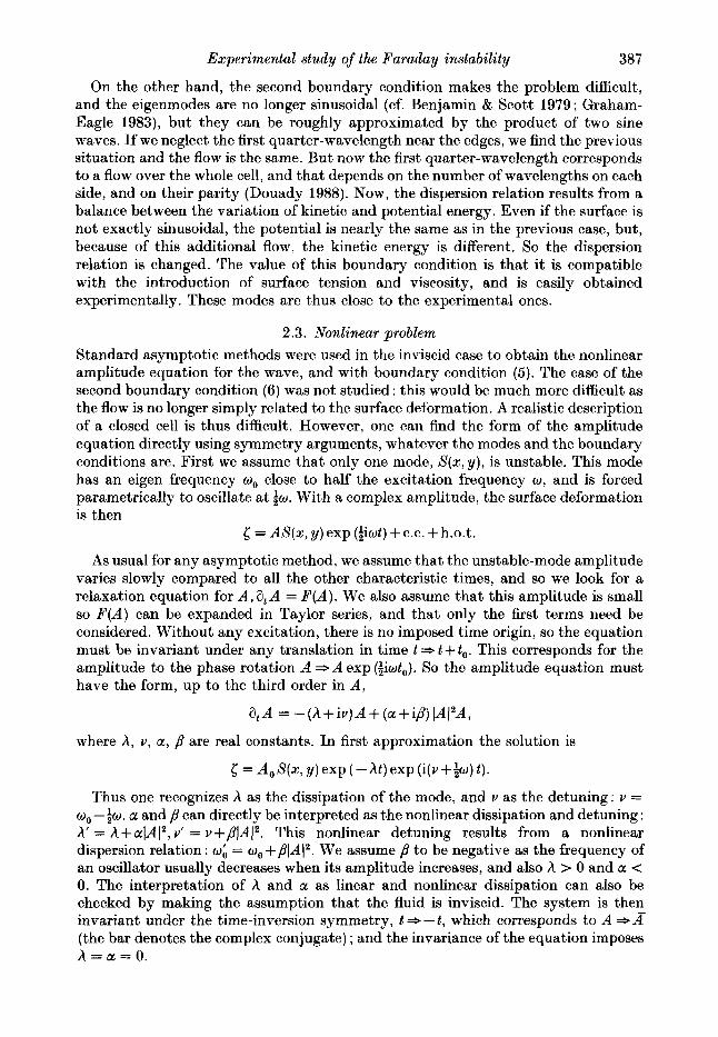
......... ........ ........................ .....+ *.. P -7 .I **...
FIQURE 3. Amplitude a and characteristic time 7 of the unstable waves versus the forcing p, in the two cases y cos (q-$) > 0 and ycos (q-$) < 0, which respectively correspond to the supercritical and subcritical transition cases.
When a forcing is applied, the continuous time translation is broken and the system only has the time translation of an excitation period: t=t+Zn/w, which correspond to A * - A . Thus one allows new terms in A, A3, lA12A, A3. We keep only the first one, so the amplitude equation becomes
The time origin is chosen in order to have p, the forcing coefficient, real. This forcing term is characteristic of parametric excitation, and comes from the wave oscillation at half the excitation frequency. This equation is well known, but as i t is usually derived in the inviscid limit, the nonlinear dissipation coefficient is often missing. This construction from symmetry arguments gives the form of the equation, but not the value of the coefficients, even if the physical interpretation is easy, We can find the linear coefficients, for instance with an asymptotic method from (1) with dissipation; this gives (Bogoluibov & Mitropolsky 1961): h =f, v = + - w 0 , p = $e' wo. The assumption that the dynamics of A is slow and A small is generally replaced
Experimental study of the Faraday instability 389
by the condition that A , v and p are small compared to oo. But this assumption upon A simply corresponds to the fact that the system is close to the minimum of the resonance tongue, which indeed implies that v is small, but only that p and h are similar. So we think that it would be possible to justify this equation with h and p not small, which is always the case experimentally.
If we look a t the stationary solutions of this equation, the arithmetic is easier with the notation
a,A = y e i ~ A + p J + c e i ~ ~ A ( 2 A . (7b)
We also decompose A into amplitude and phase: A = aexp (is), which gives
(7 c) I a = ( y cos (q) +p cos (28))a + c cos ($) a3, i"' = (ysin (q)-psin (28)) fcsin ($)a2.
For stationary solutions, we found by eliminating 0 that
ca2 = - y cos (q-$) (p2-y2 sin ( q ~ - $ ) ~ ) ; . (8)
By drawing this solution, figure 3, one sees that the transition can either be supercritical or subcritical, depending on the sign of cos (q-$), i.e. on the detuning
(i) if cos (v-$) > 0, which corresponds to v > -ha/P, the transition is super- critical. In this case, the characteristic time of the wave decay below the threshold, with the assumption that the phase remains constant, is
V :
1 /70 = - y cos (q)) k (p2 - y2 sin (P)~); ; (9)
(ii) if cos (q-$) < 0, which corresponds to v < - A alp, the transition is subcri tical.
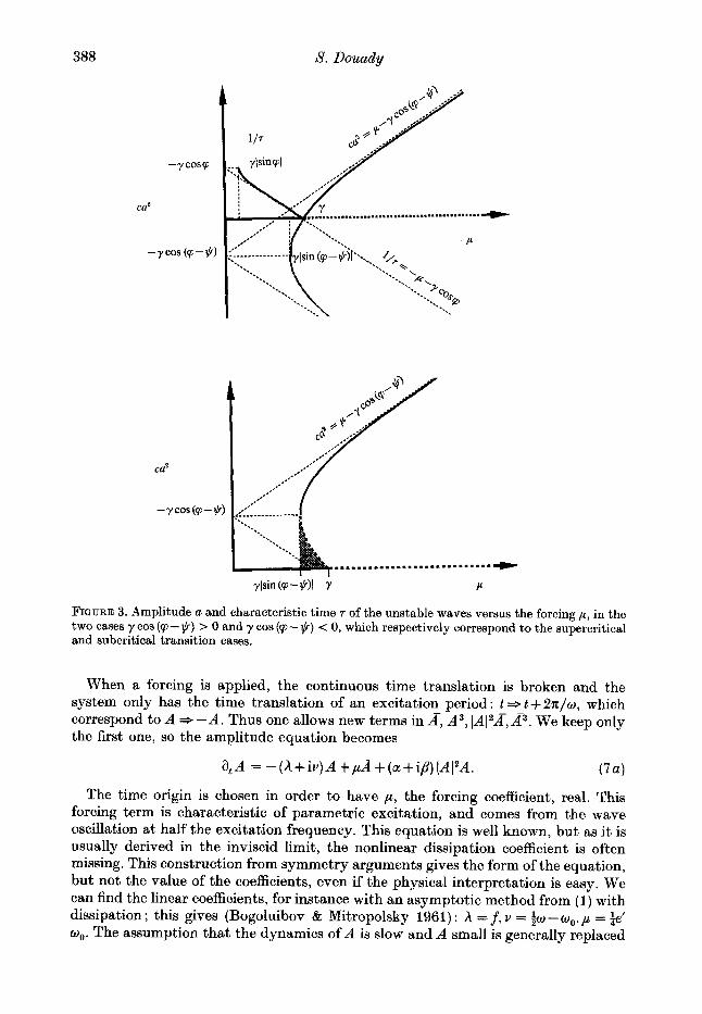
The stability of the different stationary states can be found without any further calculation by simply using the conservation of the topologic degree, i.e. the conservation of the number of stable solutions minus the number of unstable solutions (Leray & Schauder 1934), which applies to (5a) . Figure 4 summarizes the various cases in the external parameter plane. By increasing the detuning (i.e. w ) , we continuously go from a subcritical transition to a supercritical one. The existence of hysteresis is due to the nonlinear detuning coefficient p. For an excitation frequency that is too small, the mode is non-resonant for a small amplitude; but if it jumps to a significant frequency, this diminishes its eigen frequency, and thus it can resonate and become unstable. Note that this subcritical bifurcation does not need a higher-order term to saturate: if the amplitude continues to increase, the eigen frequency keeps on decreasing, so the mode is again non-resonant and the amplitude saturates. If the sign of /3 is changed, the situation is symmetric with the previous one with the hysteresis located at the right. The importance of this subcritical region is given by the ratio alp (i.e. $):
(i) if this ratio is small ($ - -in), the hysteresis is observed for w < 2w0 (Hsu 1977; Nayfeh & Mook 1979; Meron 1987; Gu & Sethna 1987), i.e. for all the left side of the tongue, and the hysteresis is maximum ;
(ii) if this ratio is significant ($ h- -n), the frequency below which the hysteresis is observed is pushed to the left, and the hysteresis becomes small (cf. figure 4). At the limit $ = -n, the transition is always supercritical (Hsu 1977).
390 S. Douady
I -Aa/p 0
(cos (c, - $) = 0) U
FIGURE 4. Stability boundaries as a function of the detuning v ( (w,-?p~) /w, , and the forcing p. The linear threshold corresponds to the hyperbola p = y and the nonlinear threshold reveals a hysteresis in the grey region. This hysteresis is at its maximum for a = 0 and disappears for /? = 0 (the transition is then always supercritical).
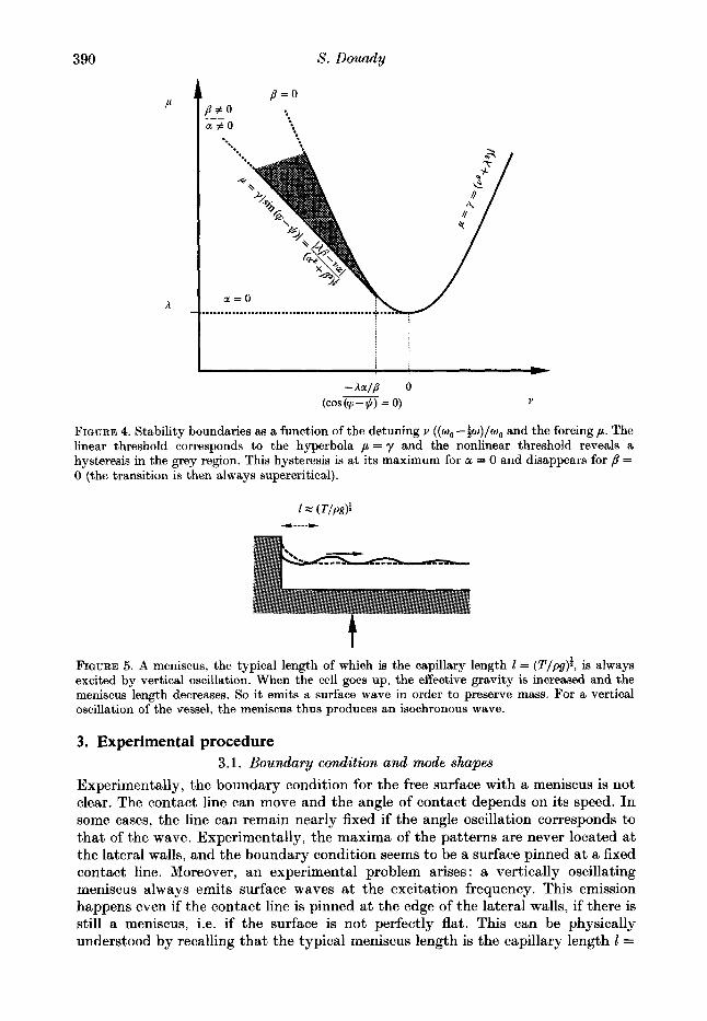
FIQURE 5. A meniscus, the typical length of which is the capillary length I = (T/pg$, is always excited by vertical oscillation. When the cell goes up, the effective gravity is increased and the meniscus length decreases. So it emits a surface wave in order to preserve mass. For a vertical oscillation of the vessel, the meniscus thus produces an isochronous wave.
3. Experimental procedure 3.1. Boundary condition and mode shapes
Experimentally, the boundary condition for the free surface with a meniscus is not clear. The contact line can move and the angle of contact depends on its speed. In some cases, the line can remain nearly fixed if the angle oscillation corresponds to that of the wave. Experimentally, the maxima of the patterns are never located at the lateral walls, and the boundary condition seems to be a surface pinned at a fixed contact line. Moreover, an experimental problem arises : a vertically oscillating meniscus always emits surface waves at the excitation frequency. This emission happens even if the contact line is pinned at the edge of the lateral walls, if there is still a meniscus, i.e. if the surface is not perfectly flat. This can be physically understood by recalling that the typical meniscus length is the capillary length 1 =
Experimental study of the Faruday instability 391
FIQURE 6. Photograph of the wave emitted by the meniscus of an oil layer of depth h = 2 mm, in a square cell 80 x 80 x 5 mm3, atf = 20 Hz, visualized by the vertical reflection of a light beam. The waves are clearly generated from the boundaries, and quickly damped, so the centre of the cell is still flat. Without any meniscus, the surface remains flat even during vertical oscillation.
(Tlpg);. In a vertical oscillation, this length oscillates like the effective gravity acceleration, so the meniscus becomes alternately large and small. In order to preserve the fluid mass, the volume difference between a small and a large meniscus must be distributed over the whole free surface, and it happens through the emission of a surface wave (cf. figure 5) . Figure 6 presents a photograph of these meniscus waves for an oil layer. Their amplitude increases with the meniscus volume and the excitation amplitude. They can cover the whole free surface when their dissipation length is larger than the cell length (for instance in water or for small excitation frequencies - 15 Hz). For the Faraday instability, these waves give a new initial condition, i.e. not a flat surface, and they modify the boundary condition. Moreover, they can greatly perturb the parametric waves as they are coupled to them at the second order, whereas two parametric waves are coupled only at the third order. Thus the modes can be completely deformed (see figure 7) , and time-dependent.
In order to avoid these problems arising from the curvature of the surface at the boundaries, one solution is to pin the surface at the edge of the lateral walls, and to fill the vessel full. The surface is then perfectly flat and remains so even when the cell oscillates vertically, below the instability threshold. The modes are then regular and stable, and can be described approximately as the product of two sine waves (cf. figure 8).
3.2. Visualization methods Vertical illumination
The simplest method consists in looking at the normal reflection of light at the free surface. One then observes bright regions which correspond to horizontal parts of the surface, extrema or saddle points. But without any optical device neither the light
392 8. Douady
FIGURE 7. An example of the patterns observed with oil with a significant meniscus, for the same conditions as figure 6, but above the instability threshold, They are nearly perfect squares near the centre of the cell, even though they are turned through a certain angle, but completely deformed at the boundaries, where the meniscus wave is still visible.
FIGURE 8. Mode observed without a meniscus, at 70 Hz, for water containing Kalliroscope. I ts regularity shows that it is quite near sinusoidal.
Experimental study of the Faraday instability 393
Bright region of nearly
Zero of the sinusoidal mode
FIQURE 9. Schematic of the bright regions observed for a product of two sine waves illuminated vertically. They correspond to the horizontal points, extrema and saddle points. When the reflection is not purely vertical, one observes segments or surfaces joining these points.
nor the observer are at infinity, so one also observes lines or surfaces joining these points (cf. figure 9). The interest of this method is the independence of time of the observed structure (so it does not need any stroboscopic observation), and the direct identification of the pattern using simple rules. The modes in a rectangular cell are described by the number of nodes in each direction, and figure 10 presents the patterns in a square cell corresponding to the mode (9,13), and the superpositions of (14,2), (14,4), and (13,7) with their respective symmetrical modes. Figure 11 shows computer drawings of the nearly horizontal regions of the surface deformation for the corresponding sinusoidal modes. In the case of a single mode, for instance figure lO(a), the two node numbers are obtained by counting the number of oblique lines along each side. In the case of a superposition of two symmetrical modes, for instance in figure 10(b,c), a larger number of modulations is obtained from the number of rapid modulating lines parallel to one side, the second number being given by the number of slow modulations. Figure 10(d) presents a case of diagonal modulations as 7/13 is larger than tan($), and corresponds to a transient state leading to one mode only, (7,13) or (13,7) (Douady & Fauve 1988).
Flow visualization Another visualization method for thin layers (Kh < 1) consists in looking at the
fluid motion revealed by small particles (for instance Kalliroscope in water). For stationary states, we principally observe a steady convection-like motion related to the surface waves: the fluid rises a t the maxima of the waves, and falls at the nodal lines (cf. figure 12). This flow is the rectified flow generated a t the viscous boundary- layer limit by the oscillatory fluid motion due to the surface waves. The acoustic streaming escapes from the maxima of horizontal velocity and converges to the minima (Batchelor 1967). This streaming had already been observed by Faraday (1831) with some sand accumulated at the cell bottom. Figure 13(a) presents a typical example of a streaming pattern, and figure 13 ( 6 ) a computer drawing of the extrema of the corresponding sinusoidal mode. This method is more complicated than the previous one, as the prediction of the extreme positions for the superposition of two sinusoidal modes is not always simple, so pattern identification is harder.
394 8. Douady
FIQURE 10. Photographs of the patterns observed in a square vessel brimful of water, with the vertical reflection of a light beam. These patterns correspond to one mode only: (a) (9,13), at f = 32.7 Hz; or to the superposition of a mode and one symmetric with i t : (21) (2,14) and (14,2), at f = 37 Hz; (c) (4,14) and (14,4), a t f = 33.8Hz; ( d ) (7,13) and (13,7), a t f = 34.2Hz.
Bicolour stroboscopy
As the surface waves oscillate at half the excitation frequency, they can resonate with two opposite phases. Thus, in a very large cell, one can imagine that two regions could oscillate in phase opposition, separated by a kink-type defect line. We thus interpret the transverse amplitude modulation observed in spatio-temporal chaos by Ezerskii et al. (1986) as these defect lines. In order to be able to verify this, we developed a phase visualization by bicolour stroboscopy . It consists in stroboscoping the surface with two complementary colours for each half-period of the wave. For the first half-period, we illuminate the surface for instance in green, and thus observe a succession of bright and black bands, corresponding to the sides of the waves being
Experimental study of the Faraday instability 395
FIQURE 11. Computer drawings of the nearly horizontal regions of the surface for the sinusoidal modes corresponding respectively to the patterns of figure 10.
FIQURE 12. Schematic of the steady flow generated by the parametric standing waves. The fluid rises at the maxima and goes down at the nodal lines. Thus the bright regions, i.e. regions of horizontal motion, correspond to level lines of the wave pattern. This flow is the steady streaming created by the viscous boundary layer a t the bottom of the cell.
396 S. Douady
FIQLJRE 13. (a) Photograph of the flow, visualized by Kalliroscope, due to the parametric wave pattern, in a square cell at f = 64 Hz for water. The surface deformation corresponds to the superposition of the mode (21,4) and a symmetric one. It shows the ‘level lines’ of this pattern. ( b ) Computer drawing of the ’level lines ’ for the corresponding sinusoidal pattern, black corresponding to a surface deformation greater than a certain value.
Journal of Fluid Mechanics, Vol. 221 Plate 1
FIGURE 15. Pattern photographs with bicolour stroboscopy in a square cell atf=70 Hz. (a) The transient state when the mode (21,5) starts to increase; (b) the final state corresponding to the superposition of the two square symmetrical modes. This method visualizes the phase opposition between two regions separated by what seem to be defect lines, as the two colours are exchanged when one crosses these lines.
DOUADY (Facing p . 397)
Experimental study of the Faraday instability
f* Light beam ,#
1 Free surface
Cell bottom
Top view
397
t
Red ...........
t -k $To
FIGURE 14. Principle of bicolour stroboscopy visualization. It consists in looking at the reflection of a light beam which alternately changes colour at each excitation period T. For half a resonant wave period 4% (= T), the wave is illuminated in green, and for the other half-period in red. Thus we observe alternating green and red bands.
turned or not to the light (cf. figure 14). For the other half-period, we illuminate for instance in red, and the black and bright regions are exchanged. Thus, for a plane wave, we observe an alternation of green and red bands with a periodicity of one wavelength (cf. figure 15a, plate 1). The phase of the local structure is given by the fact that a point is green or red, and we observe the phase opposition when one crosses each transverse modulation line of figure 15 (a) , as red is changed into green and green into red. This phase opposition is also verified when one crosses each vertical or horizontal modulating line in figure 15b, plate 1).
In fact, for these figures, the modes are nearly the product of two sine waves, and what seems to be a transverse modulation of a plane wave in figure 15(a) merely corresponds to the slow and rapid modulation of these products : figure 15 (a ) presents the transient of the mode (21,5) growing alone, and figure 15(b) the final state of the superposition of the two symmetric modes. So we cannot strictly speak of defect lines in these cases, even if they behave like during transient states. But we think that for a larger cell (or for a small wavelength), this method could be used to show that the observed transverse modulation corresponds to the appearance of these defect lines.
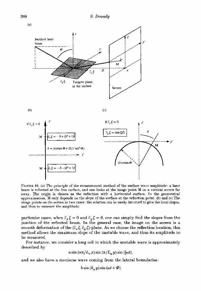
3.3. Amplitude measurement method The method consists in looking at the image on a vertical screen of a thin laser beam reflected a t the free surface. In the geometrical approximation, and if the screen is far enough away, the position of the reflected beam depends only on the surface slope at the reflection point. Figure 16 presents the principle and notation. In two
398
(4
8. Douady
Incident laser beam
L
*.-- -*' ay[ Tangent plane
at the surface
if aY[ = 0
M
Z'
b = (cotan 8 + D/z' sin2 S ) - Y , ... ___.__..__---...._..---.....
Screen / A if = 0
FIQURE 16. (a ) The principle of the measurement method of the surface wave amplitude: a laser beam is reflected at the free surface, and one looks at the image point M on a vertical screen far away. The origin is chosen as the reflection with a horizontal surface. In the geometrical approximation, M only depends on the slope of the surface a t the reflection point. ( b ) and ( c ) The image points on the screen in two cases : the relation can be easily inverted to give the local slopes, and thus to measure the amplitude.
particular cases, when a, 6 = 0 and a, 5 = 0, one can simply find the slopes from the position of the reflected beam. I n the general case, the image on the screen is a smooth deformation of the (a, 5, a, c)-plane. As we choose the reflection location, this method allows the maximum slope of the unstable wave, and thus its amplitude to be measured.
For instance, we consider a long cell in which the unstable wave is approximately descri bed by
and we also have a meniscus wave coming from the lateral boundaries:
a sin (nz/L,z) sin (z/L,y) sin (!pwt),
b sin (ky y) sin (ot + @)
Experimental study of the Ir'araday instability 399
FIGURE 17. Image obtained on the screen for a vessel almost brimful with water. The reflection point is located at a node for both the parametric and meniscus waves. So the image point M describes a Lissajous curve showing the ratio 2 between the frequencies of the two standing waves. The extreme vertical points gives the amplitude of the parametric wave.
(cf. figure 18). We put the laser beam along the x-direction, and a t the middle of the cell @,sin (n/L,y) = 0). At this location, the slopes are
a, 5 = uK, cos (K,x) sin (tot), a, g = bk, cos (k, y) sin (ot + @),
with K , = nn/L,. The light on the screen thus describes a Lissajou curve, as in figure 17. To obtain only the slope of the unstable mode, we move the reflection point to a maximum of the meniscus wave (cos (ku y) = 0) , and to a node of the unstable mode :
a,[=aK,sin(!pt), a , [ = O .
So the reflected beam oscillates between two extreme vertical positions, which gives the maximum slope, i.e. the amplitude of the wave. As far as we know this method is new. It provides very sensitive measurements (resolution better than mm) as we use the reflection of a light beam, and is especially useful for small wave amplitudes (a,[ -= l / tan(tO)).
400 8. Douady
3.4. Experimental procedure In spite of the simplicity of a vertically oscillating layer of fluid, experimental problems arise from the meniscus effects, the mechanical set-up, and the variation of the fluid properties :
(i) We have seen that the meniscus is important as it generates surface waves which can perturb the parametric standing surface waves. There is no general solution for this problem. For a moderately wetting fluid, such as water, one can pin the free surface a t the edge of the lateral walls to obtain a perfectly flat surface. In our experiments with oil, we used a long cell in order to separate easily the resonant wave from the meniscus one.
(ii) Like the meniscus, horizontal motion generates propagating waves from the sidewalls. Rolling motion must also be eliminated in order to have the same amplitude excitation in the entire vessel, and thus the same amplitude of the resonant wave. So the motion must be purely vertical. The fluid depth must be constant (i.e. the vessel must be horizontal). If any of these conditions is not fulfilled, the waves can be non-stationary and slowly move, coupled to a large-scale steady flow. A simple test for the mechanical system is to use a vessel brimful of water, and to check that the surface remains perfectly flat just below the instability threshold. The excitation homogeneity is also easily visible just above the threshold.
(iii) The stability of the experiment over a long time depends on the stability of all the fluid-layer characteristics : the fluid depth h, surface tension T , and viscosity (i.e. dissipation). Thus the system must be thermally regulated, and, for a volatile fluid, the atmosphere must be saturated in the fluid vapour to avoid evaporation.
4. Experiments 4.1. Experimental set-up
We used a Briiel & Kjaer 4809 vibration exciter which produces a clean vertical acceleration waveform (the horizontal acceleration is less than 1 % of the vertical one). The vibration exciter is driven by a Krohn-hite frequency synthesizer (frequency precision better than The cell acceleration, which is the relevant bifurcation parameter, is measured with an accelerometer. The mechanical system was tested with a vessel brimful of water: the surface remained perfectly flat just below the threshold, and just above, the amplitude was everywhere the same.
To study the threshold of the instability, we used a copper vessel of dimension 65 x 16 x 5 mm3, thermally regulated. We varied the excitation frequency between 20 and 30 Hz. The first fluid used was a silicon oil (Rhodorsil47V20), a t 30 "C, chosen for the stability of its surface tension and non-volatility. As it wets the cell walls, the oil has a significant meniscus. But the geometry of the cell, a long rectangle, was chosen in order to separate the meniscus and the parametric wave, as the meniscus wave is important only along the lateral walls (the wave due to the nearly round meniscus is quickly damped), contrary to the parametric wave (cf. figure 18), which presents several modulations in the long direction and only one perpendicularly. Even in this case, the modes shape are similar to the product of two sine waves, so the real boundary condition seems to be close to a virtual pinning a t the meniscus. We also used this cell filled up with water, then held at 5 "C, to study the influence of the boundary condition.
Experimental study of the Faraday instability
.- c)
2
d 3 10-
40 1
-- . -0-
12 _- _ - ._I-. -__-- -
Meniscus
Resonant wave
n = 12
4 D
65 mm
FIQURE 18. Experimental vessel used for the study of the threshold. In the case of a significant meniscus (with oil) the isochronous standing meniscus wave shows modulations along the small dimension, and the half-frequency parametric standing wave is seen along the large dimension.
-- 1
l 3 1 h
R 13
- I 15 _ - I- - - - -
8 ! a I I I I I 1
28 30 32 34 36 38 40 42
Excitation frequency (Hz)
FIGURE 19. Stability boundaries for oil for two fluid depths h. Each measurement corresponds to two points, one below and one above the threshold. The precision does not allow us to distinguish them on this figure. The 4 tongues of the modes with 11-15 modulations in the long direction are observed. The threshold increases with the frequency (cf. (2)) and decreases when the fluid depth is increased, showing that the dissipation principally depends on the friction a t the waIls, including the bottom.
4.2. Threshold The threshold is measured for a fixed frequency, by starting with an amplitude excitation corresponding to a parametric wave of large amplitude. Then, we slowly decrease it in order to obtain a small amplitude, corresponding to a few centimetres
FIGURE 20. Stability boundaries for water, for a case of almost no meniscus. The resonance tongues are well defined for different modes (m, n), where m and n are the number of modulations in each dimension. Two series are observed corresponding to one or two modulations in the small dimension, with respective critical-value series increasing.
deviation of the reflected laser beam on the screen located 1 m away (i.e. a, 5 x 2 lo-' and a x 5 x mm). Then we note a first value of the amplitude excitation a t which the wave amplitude increases, and a second at which it decreases. For this lower value, we can check that the amplitude goes to zero if we wait long enough. In this way, we quickly obtain two points, below and above the threshold, with a good precision, as the typical difference is 0.2%.
Figure 19 presents two threshold curves obtained for two oil depth, h = 2.25 and 2.40 f 0.05 mm. One can recognize for each curve the various instability tongues corresponding to the modes n = 11 to 15, with only one transverse modulation. Figure 20 presents the threshold curve for a vessel nearly brimful of water (h = 4.85 mm), and two series of instability tongues, corresponding to modes with one or two transverse modulations, are observed.
4.3. Dissipation, eigen frequency and boundary effects From the theoretical analysis, we have seen that the minimum of the instability tongue gives the characteristics of the surface wave mode, as this tongue is centred on the double-eigen frequency, and that the critical value of the excitation is proportional to the dissipation of the mode. But this is true only when the tongue is plotted in the physical parameter space (acceleration versus frequency), and the physical meaning of the minimum is lost when the tongue is plotted in terms of other quantities, for instance velocity, or displacement, versus frequency.
Thus, from the curves one can read the dissipation of the various modes directly. In figure 19, the critical value of the tongues increases quickly with frequency, as it is harder to excite capillary waves than gravity ones (cf. (4)). The distinction between the tongues becomes less clear, and for higher frequencies one only observes a continuous increase of the threshold with frequency. The two curves obtained for different fluid depth show the great sensitivity of the system to possible evaporation, and that the dissipation, increasing with decreasing depth, is mainly due to the friction a t the lateral walls. In figure 20, the threshold also increases with frequency
Experimental study of the Faraday instability 403
for each series of tongues, but one mainly observes the difference between the two series. The increase of dissipation for modes with increasing numbers of transverse modulations was also observed in a square cell (Douady & Fauve 1988), and explains why modes with a larger number of transverse modulations are not observed in water or in oil. This is a direct consequence of the real boundary condition of the free surface.
Concerning the shape of the tongues, one can see that the tongues obtained without a meniscus in water can be fitted with a parabola (corresponding to the development of the theoretical hyperbola), and that the intersection between two tongues is sharp, contrary to the curves obtained with an oil meniscus, where the intersection is smooth. This corresponds exactly to the shape of the eigenmodes, which are well defined and fixed in case of edge constraint, but which can be continuously deformed from one another when there is a meniscus. The position of the nodes is then experimentally observed to move continuously with the excitation frequency.
Figure 20 also shows that the dispersion relation is modified by the boundary condition from the infinite case (equation (2)). As the observed modes are close to the product of two sine waves, the corresponding wavenumber can be easily estimated from the two modulation numbers (m, n ) :
For our experiments, the dispersion relation is monotonic, so the modes should be observed when increasing the excitation frequency by the increasing order of the wavenumber: (7, l), (3,2), ( 8 , l ) quite near (4,2), (5,2), (9, l), and (6,2). But experimentally figure 20 presents a different order: (4,2), (7, l), (5,2), (8, l), (6,2), and (9 , l ) . This corresponds to the shift of one series of tongues with respect to the other, not only for the eigen frequencies, but also for the dissipation. This shows that the flow inside the fluid is influenced by the lateral walls, so that the eigen frequency and the dissipation depend not only on the total wavenumber but also on the structure of the mode (Benjamin & Scott 1979; Graham-Eagle 1983; Douady 1988).
However, this effect of the boundary condition for the free surface on the eigen frequency must disappear when the cell, i.e. when the wavelength, becomes large. In a long cell, 138.2 x 14 x 48 mm3, filled with water, we observed modes with only one transverse modulation, but a large number of periodic ones in the long dimension (always more than 20). As we used felt to cover the lateral walls, there was almost no meniscus and the surface was approximately pinned. The frequency, between 30 and 200 Hz, is large enough that the wavelength in the long dimension is always smaller than the width of the cell, so K , K . The curved obtained by plotting the measured wavelength versus half the excitation frequency (cf. fig. 21) can be fitted by the dispersion relation (2), by adjusting the only unknown experimental parameter, the surface tension. This is thus a way to measure surface tension, and for water with traces of ink and Kalliroscope (containing soap), we obtained T = 29.5 dyn/cm.
4.4. Amplitude and characteristic time With the reflected laser beam, we measure the static amplitude of the unstable wave above the threshold, but we can also measure the characteristic time of decay of the amplitude when the acceleration is suddenly decreased to 8 value below the threshold. The time record of the laser beam position on the screen shows that the decay of the amplitude is exponential, which is consistent with the above assumption
FIGURE 21. Experimental measurements of the unstable-mode wavelength versus the excitation frequency, in polluted water. This curve can be perfectly fitted, and this gives a measurement of the surface tension, which is found to be T = 29.5 dyn/cm.
Acceleration modulation (m/s')
FIGURE 22. Experimental measurements of the wave amplitude and characteristic time versus the acceleration, for three frequencies, for the tongue n = 12 and h = 2.4 mm of figure 19. The amplitude presents no hysteresis and the characteristic time diverges at the threshold, so the transition is supercritical.
of a constant phase during the decay. We also confirmed that the corresponding characteristic time depends only on the distance from threshold of the final acceleration.
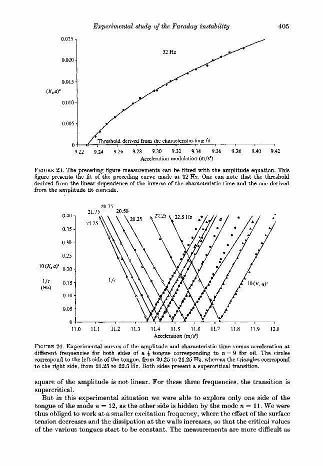
Figure 22 shows three measurements of amplitude and characteristic time at different frequencies for the mode n = 12 of figure 19. The characteristic time 7 diverges very quickly when approaching the threshold: the wave takes only two seconds to disappear at 3% below the threshold, but half a minute at 0.5%. l / t is proportional to the distance from threshold. Figure 23 shows that the increase of the
Experimental study of the Faraday instability 405
32 Hz // /
I/ /’
/*
/(ihresho!d derive! from t p charayteristic-:me fit I I I I
FIQURE 23. The preceding figure measurements can be fitted with the amplitude equation. This figure presents the fit of the preceding curve made at 32 Hz. One can note that the threshold derived from the linear dependence of the inverse of the characteristic time and the one derived from the amplitude fit coincide.
FIGURE 24. Experimental curves of the amplitude and characteristic time versus acceleration at different frequencies for both sides of a t tongue corresponding to n = 9 for oil. The circles correspond to the left side of the tongue, from 20.25 to 21.25 Hz, whereas the triangles correspond to the right side, from 21.25 to 22.5 Hz. Both sides present a supercritical transition.
square of the amplitude is not linear. For these three frequencies, the transition is supercritical.
But in this experimental situation we were able to explore only one side of the tongue of the mode n = 12, as the other side is hidden by the mode n = 11. We were thus obliged to work at a smaller excitation frequency, where the effect of the surface tension decreases and the dissipation at the walls increases, so that the critical values of the various tongues start to be constant. The measurements are more difficult as
FIGURE 25. One of the amplitude curves from the preceding figure showing the linear saturation of the amplitude versus acceleration modulation (higher-order terms must be retained in the amplitude equation).
TABLE 1 . The coefficients of the amplitude equation for n = 12. p, is the ratio between the forcing coefficient ,a and the acceleration modulation gm (the effective gravity is g+gm cosot). Equation (4) is non-dimensionalized with T = ot and a’ = K,a (cf. $2.3). The value of I Y I is zero up to the precision 5 x 10⁻⁴.
the meniscus wave in the long dimension starts to be visible, and the amplitude of the unstable wave becomes noisy, probably because of . their interaction. For measurements made a t very small amplitude, for instance of the characteristic time, we were then obliged to subtract the amplitude of the meniscus waves. Figure 24 presents a study of the mode n = 9, around 20 Hz. In this case, both the inverse of the characteristic time and the square of the amplitude are proportional to the distance from threshold. Figure 25 shows the linear saturation of the amplitude with the acceleration far above the threshold. All the transitions, for both sides of the tongue, are supercritical.
All these curves can be fitted with the theoretical expressions (8) and (9). Figure 23 presents the measurements and a fitted curve obtained by adjusting the amplitude equation coefficients. One can note the agreement between the two thresholds derived by the fit of the amplitude and by the characteristic time. From both fits, we can obtain all the coefficients of the amplitude equation, which are shown in table 1 for each curve of figure 22. As the inverse of the characteristic time is proportional to the distance from the threshold, one directly knows that the detuning v (= ysinq) is small (cf. fig. 3).
I n the case of the mode n = 9, the linearity of both the inverse of the characteristic time and the square of the amplitude versus the distance from threshold shows that
TABLE 2. As table 1, but for n = 9, which requires the assumption that = 0
both the detuning v and the nonlinear detuning pare small (cf. fig. 3). But in this case the two fits do not provide enough information to derive completely the amplitude equation parameters. We thus need an assumption, which is to assume /3 equal to zero, and the corresponding result is presented in table 2.
The first conclusion of this study is that the amplitude equation derived from symmetry arguments can describe the behaviour in the vicinity of instability onset, whatever the real surface wave modes are. Second, we see that we are able to obtain from the measurements the coefficient of the amplitude equation, and thus to obtain complete information on the surface wave modes. The dissipation is of the order of magnitude of the dissipation due to the solid wall h - K(vw)i, which, for w/2n x 30 Hz, 2nK x 2 cm, v = 2 lop5 m2 s-', gives h/w - 0.1. If one assumes that the coefficient pr is the same for water and oil, then the ratio between the two thresholds is approximately the square root of the ratio between the viscosities, 4 2 0 , so with a threshold for oil of 11 ms-2, one obtains for water a threshold of 2.5msp2 (cf. figures 19, 20). One can see that despite the decrease of dissipation with frequency, as the friction at the walls decreases, the threshold increases, because of the difficulty of exciting capillary waves with gravity modulations (cf. (4)). The nonlinear dissipation is comparable with the linear, even if it seems to decrease more quickly with frequency. On the other hand, the nonlinear detuning increases with frequency, which is a classical result as Stokes derived a dependence in K2.
All the transitions observed were supercritical, and this corresponds of course to the coefficients derived. At small frequencies, where both sides of the tongue can be studied, p is too small (cf. table 2) ; and a t higher frequencies, we found a small and p important (cf. table l), so an hysteresis is possible on the left side of the tongue, but it cannot be observed as this part is hidden by another tongue. For the experiments with water, the transition was always observed to be supercritical on both sides of the tongue, although it becomes steeper a t the left. But amplitude measurements were difficult in these regions because of mode interactions (cf. Ciliberto & Gollub 1984, 1985).
The main information from tables 1 and 2 is that the detuning is always negligible compared to the frequency variation. This means that the mode is always resonant, w = 2w,, in other words that the mode is continuously deformed in order to adapt its eigen frequency continuously. This is possible because of the complex boundary condition for the free surface due to the meniscus.
408 S. Douady
5. Conclusion This study shows that parametrically excited waves are very sensitive to the free-
surface boundary condition. With a meniscus, the vertical oscillation emits a surface wave at the excitation frequency which interferes with the parametric wave. Also, the real boundary condition is unclear in this situation, and our experiments show that the surface wave mode can be continuously deformed in order to stay at resonance for any excitation frequency. On the other hand, when the surface is pinned at the edge of the lateral walls, and the cell filled full, we obtain a perfectly flat surface and the modes are well defined.
But although a complete and realistic hydrodynamical description of the unstable modes is difficult, one can simply describe their dynamics with an amplitude equation derived with symmetry arguments. Its predictions are in good agreement with the experiments, and the coefficients of this equation were derived. As this method naturally takes into account the nonlinear dissipation, it explains why the observed transition is always supercritical.
Finally, we note that the study of the threshold of this instability is a simple way to study the surface wave modes of a closed vessel:
(i) the minimum of the tongue gives the dissipation and the eigen frequency of the unstable mode. We thus observed the effect on both of the edge constraints as a dependence on the structure of the mode, i.e. on the respective number of modulations in each direction of the rectangular cell, and not only on the total wavenumber ;
(ii) the derived amplitude equation coefficients also give the nonlinear dissipation, and the dependence of the eigen frequency on the amplitude.
We particularly thank S. Fauve for many helpful discussions throughout the development of these experiments. We thank the Dret for support under contract 86/1518. During the revision of this paper, we benefitted from a project done at the GFD Summer Study Program, on ‘hydrodynamic waves of a brimful vessel with edge constraint’. We acknowledge W. R. Young for proposing and directing this project, and the GFD program of the Woods Hole Oceanographic Institution for support.
REFERENCES
BATCHELOR, G. K. 1967 A n introduction to Fluid Dynamics. $5.13. Cambridge University Press, BENJAMIN, T. B. & SCOTT, J. C. 1979 Gravity-capillary waves with edge constraints. J . Fluid
BENJAMIN, T. B. & URSELL, F. 1954 The stability of the plane free surface of a liquid in vertical
BOGOLIUBOV, N. N. & MITROPOLSKY, Y. A. 1961 Asymptotic Methods in the Theory of Non-Linear
CILIBERTO, S. & GOLLUB, J. P. 1984 Pattern competition leads to chaos, Phys. Rev, Lett. 52,
CILIBERTO, S. & GOLLUB, J. P. 1985 Chaotic mode competition in parametrically forced surface
DOUADY, S. 1988 Capillary-gravity surface wave modes in a closed vessel with edge constraint :
DOUADY, S. & FAWE, S. 1988 Pattern selection in Faraday instability. Europhys. Lett. 6,221-226.
Mech. 92, 241-267.
periodic motion. Proc. R. SOC. Lond. A 225, 505-515.
Oscillations, p. 267-284. Gordon & Breach.
922-925.
wavea. J . Fluid Mech. 158, 381-398.
eigen-frequency and dissipation. Woods Hole Ocean. Inst. Tech. Rep. WHOI-88-26.
Experimental study of the Faraday instability 409
EZERSKII, A. B., KOROTIN, P. I. t RABINOVITCH, M. I . 1985 Random self-modulation of two- dimensional structures on a liquid surface during parametric excitation. Zh. Eksp. Teor. Fiz. 41, 129-131 (transl. Sov. Phys. JETP 41, 157-160 (1986)).
EZERSKII, A. B., RABINOVICH, M. I., REUTOV, V. P. t STAROBINETS, I. M. 1986 Spatiotemporal chaos in the parametric excitation of a capillary ripple. Zh. Eksp. Teor. Fiz. 91, 2070-2083 (transl. Sov. Phys. JETP 64, 1228-1236 (1986)).
FARADAY, M. 1831 On the forms and states of fluids on vibrating elastic surfaces. Phil. Trans. R . SOC. Lond. 52, 31S340.
GOLLUB, J. P. t MEYER, C. W. 1983 Symmetry-breaking instabilities on a fluid surface. Physica
GRAHAM-EAGLE, J. G. 1983 A new method for calculating eigenvalues with application to gravity-
Gu, X. M. t SETHNA, P. R. 1987 Resonant surface waves and chaotic phenomena. J . FZuidMech.
Hsu, C. S. 1977 On nonlinear parametric excitation problems. Adv. Appl. Mech. 17, 24&302. KEOLIAN, R., TURKEVICH, L. A., PUTTERMAN, S. J., RUDNICK, I. t RUDNICK, J .A. 1984
Subharmonic sequences in the Faraday experiment : departure from period doubling. Phys. Rev. Lett. 47, 1133-1 136.
LERAY, J. & SCHAUDER, J. 1934 Topologie et equations fonctionnelles. Ann. Sci. Ecole Norm. Sup. (3) 51, 45-78.
MERON, E. 1987 Parametric excitation of multimode dissipative systems. Phys. Rev. A 35, 48924895.
MERON, E. & PROCACCIA, I. 1986a Theory of chaos in surface waves: the reduction from hydrodynamics to few-dimensional dynamics. Phys. Rev, Lett. 56, 1323-1326.
MERON, E. & PROCACCIA, I. 1986b Low-dimensional chaos in surface waves: theoretical analysis of an experiment. Phys. Rev. A 34, 3221-3237.
MILES, J. W. 1984 Nonlinear Faraday resonance. J . Fluid Mech. 146, 285-302. NAYFEH, A. H. t MOOK, D. T. 1979 Nonlinear Oscillations, 8 1.5 and 5.7.3. Wiley. RAYLEIQH, LORD 1883 On the crispation of fluid resting upon a vibrating support. Phil. Mag. 15,
WHITHAM, G. B. 1974 Linear and Nonlinear Waves. Wiley-Interscience. Wu, J., KEOLIAN, R. & RUDNICK, I. 1984 Observation of a nonpropagating hydrodynamic
D 6, 337-346.
capillary waves with edge constraints. Math. Proc. Camb. Phil. SOC. 94, 553-564.