Experimental Study of the parameters affecting the...

Exp

erimen

tal S

tud

y o

f the p

ara

meters a

ffectin

g th

e kin

etics of co

alesc

ence

of m

ilk d

rop

s

Lara

Ven

tura

Experimental Study of the

parameters affecting the kinetics

of coalescence of milk drops

Lara Ventura

UNIVERSITÀ DEGLI STUDI DI SALERNO

Facoltà di Ingegneria

Dipartimento di Ingegneria Industriale

Corso di Laurea in Ingegneria Alimentare

Experimental Study of the parameters affecting

the kinetics of coalescence of milk drops

Master’s Thesis in Food Engineering

Relatori: Candidato:

Prof. Ing. Gaetano Lamberti Lara Ventura

Prof. Ing. Lilia Ahrnè matricola:0622800149

Correlatore:

Ing. Loredana Malafronte

Anno Accademico 2014/2015

Part of this thesis work has been developed during the

Erasmus project at the Chalmers Technical University, in

Gothenburg, Sweden.

It has been performed both at the Department of Process and

Technology Development of SP The Swedish Institute for Food and

Bioscience, under the supervision of Prof. Lilia Arnhè and the PhD

candidate LoredanaMalafronte, and at Chalmers University under the

supervision of Dr. RomainBordes.

Parte del lavoro di tesi è stato sviluppata nell’ambito del

progetto Erasmus presso la Chalmers Technical University, in

Gothenburg, Svezia.

In particolare, le attività di ricerca sono state svolte sia presso il

Dipartimento di Process and Technology Development del SP The

SwedishInstitute for Food and Bioscience, sotto la supervisione della

Prof.ssa Lilia Arnhè e della dottoranda Loredana Malafronte, sia

alla Chalmerssotto la supervisione di Romain Bordes.

Questo testo è stato stampato in proprio, in Times New Roman

La data prevista per la discussione della tesi è il 23/09/2015

Fisciano, 18/09/2015

[I]

Contents

Contents ................................................................................ I

Figures Index ...................................................................... V

Tables Index ...................................................................... IX

Sommario .......................................................................... XI

Abstract .......................................................................... XIII

Introduction ......................................................................... 1

1.1 Spray Drying ____________________________________ 2

1.2 Collision ________________________________________ 3

1.2.1 Explanation of the binary drop collision phenomenon 4

1.3 Coalescence ____________________________________ 11

1.3.1 Experimental methods to study coalescence 11

1.4 Key Parameters _________________________________ 16

1.4.1 Surface tension 17

1.4.2Contact angle 19

1.5 Aims of the thesis _______________________________ 22

Material & Methods .......................................................... 23

2.1 Materials ______________________________________ 24

2.1.1 Milli–Q Water 24

2.1.2 Milk 24

Pag. II Study of the Parameters affecting the coalescence Lara Ventura

2.1.3Teflon 24

2.2 Equipment_____________________________________ 25

2.2.1 Freeze Drying 25

2.2.2 Optical Tensiometer 26

2.3 Methods _______________________________________ 27

2.3.1 Samples’ preparation 27

2.3.2 First configuration. 29

2.3.3 Second configuration 31

2.3.4 Simulation of Process of Coalescence 32

Modeling & Coding .......................................................... 35

3.1 Overview of Drop Shape Techniques ________________ 36

3.2 Code steps _____________________________________ 40

3.2.1 Introduction 40

3.2.2 Image Acquisition. 42

3.2.3 Edge detection 43

3.2.4 Fitting with an ellipse 48

3.2.5 Substrate identification 50

3.2.6 Physical Properties of sample 52

3.2.7 Adimensionalization 53

3.2.8 Construction of Laplace profile 54

3.2.9 Evaluation of the error function 57

3.2.10 Numerical Optimization 58

Results & Discussion ......................................................... 61

4.1 Surface tension analysis by optical tensiometer ________ 62

4.2 Contact angle analysis by optical tensiometer__________ 63

4.3 Coalescence analysis _____________________________ 65

4.3.1 Optical tensiometer 65

4.3.2 Matlab 67

Conclusions ........................................................................ 77

Index Pag. III

Appendix ............................................................................ 81

A.1 Contact Angle Analyzer __________________________ 82

A.1.1 Implementation 82

B.1 Program Code __________________________________ 85

%B.1.1 Extraction of frames 85

%B.1.2 Movie analysis 86

%B.1.3 Determining the contact Angle on a Substrate 87

References .......................................................................... 99

Acknowledgements .......................................................... 103

Pag. IV Study of the Parameters affecting the coalescence Lara Ventura

Index Pag. V

Figures Index

Figure 1:SEM-photograph of spray dried and agglomerated powder......................... 3

Figure 2: Terminology of possible droplet collision outcomes .................................. 4

Figure 3: Schematic of the collision of two moving drops, with velocities u 1

and us, diameters d1 and ds, colliding with a collision angle of α, and an impact

parameter X. ............................................................................................................... 5

Figure 4: Analytically obtained regions of coalescence, reflexive separation, and

stretching separation for drop size ratio Δ=1.0 together with experimental

data(+, stretching separation, ...................................................................................... 7

Figure 5:Schematic of reflexive separation of two equal-size drops (a)..................... 8

Figure 6: Motion of the surface point located on the (a) z-axis (b) r-axis for

different Reynolds numbers in head-on collision of two equal-size drops with

urel=2 ........................................................................................................................... 9

Figure 7: Time resoloved shape evolution of the head-on collision of two equal-

size drops with urel=2: (a) Re=5, (b) Re=30, and (c) Re=60.The numbers on the

figure represent the time ........................................................................................... 10

Figure 8:Skecth of (a) coalescence process in condensation experiment, (b)

coalescence process in syringe deposition experiment; (c, d) spreading of drop

in syringe deposition experiment. ............................................................................. 12

Figure 9:The relaxation time tcvariations with equilibrium drop radius R for

condensation and syringe experiments on polyethylene (log-log plot). The

syringe data correspond to different temperature of the substrate around the

room dew temperature (TD= 13°C). Open circles: condensation; open triangles:

syringe, Ts=TD+5°C; open square: syringe, Ts=TD; full squares; syringe, Ts=TD-

5°C. Full line: best fit of the data at Ts=TD+5°C to Eq. (10). Broken line: best fit

of the data at TS= TD-5°C to Eq. (10). Dotted line: the best fit of the data at

Ts=TD to Eq. (10). .................................................................................................... 14

Figure 10: Evolution of HL(open circles), HR (full circles) and 2Ry (full

triangles) in a semi-log plot. The broken lines are teh fits to Eq. (11) and the full

line to Eq. (9), with A=0. .......................................................................................... 15

Pag. VI Study of the Parameters affecting the coalescence Lara Ventura

Figure 11: Selected contact angle relaxation results for C12E5solutions on

polyethylene ............................................................................................................. 16

Figure 12: Kinetic of contact angle relaxation for 1x 10^-4 M C12E6 solution on

polyethylene.............................................................................................................. 17

Figure 13: The apparent effect of fat content on surface tension. ............................. 18

Figure 14: Schematic representation of capillary method. The height, h, that

liquid will rise is linked to the contact angle, θ, and the radius of the tube, r. .......... 18

Figure 15:Illustration of contact angles formed by sessile liquid drops on a solid

surface....................................................................................................................... 19

Figure 16: Scheme of Wilhelmy Plate ...................................................................... 20

Figure 17: General layout of a Freeze Dryer: (1) top shelf, (2) Drying chamber,

(3) Usable shelves, (4) Condenser, (5) Condenser Chamber, (6): Vacuum

pumping system ........................................................................................................ 25

Figure 18: Alpha 1-2 LD Plus Freeze Dryer ............................................................. 26

Figure 19: Attension Optical Tensiometer, Theta Lite ............................................. 27

Figure 20: Surface tension measurements: (1) water droplet, (2) milk at 90% of

water content, (3) milk at 70% of water content ....................................................... 29

Figure 21: A basic experimental setup ..................................................................... 30

Figure 22: Picture from Software Attension ............................................................. 30

Figure 23: Contact angle measurements: (1) Water droplet,(2) Milk at 90% of

water content, (3) milk at 70% of water content ....................................................... 31

Figure 24: Fitting of a drop from an optical tensiometer .......................................... 31

Figure 25: Steps coalescence's process ..................................................................... 33

Figure 26: Coordinate system used to solve the Laplace-Young equation

showing the relationship between X, Z, S and θ. ...................................................... 39

Figure 27:Variation in drop shape with respect to dimensionless radius of

curvature at apex, B. ................................................................................................. 39

Figure 28: Schematic procedure fotMatlab's code .................................................... 40

Figure 29: Sessile Drop ............................................................................................ 41

Figure 30: Black and White Image .......................................................................... 42

Figure 31: Intensity graph of a signal ....................................................................... 44

Figure 32: First derivative of the signal .................................................................... 45

Figure 33: Sobel detector .......................................................................................... 47

Figure 34: Drop's profile .......................................................................................... 48

Figure 35: Schematic representation of the ellipse ................................................... 49

Index Pag. VII

Figure 36:Trial and error procedure, black line for experimental profile and the

blue one for ellipse, in which there is a variation of the parameters......................... 49

Figure 37: Fitting with ellipse, blu curve for experimental data and red for

ellipse. ...................................................................................................................... 51

Figure 38: Identification of apex .............................................................................. 52

Figure 39: Transformation of the coordinate system ................................................ 54

Figure 40: Calculation of error over the drop profile ............................................... 56

Figure 41:b against error .......................................................................................... 59

Figure 42:Fitting drop with Laplace-Young curve ................................................... 59

Figure 43: Surface tension against solid content ...................................................... 62

Figure 44: Contact angle versus solid content .......................................................... 63

Figure 45: Example ofcoalesce kinetics of water and concentrated skim milk

75% .......................................................................................................................... 65

Figure 46: Water, left angle ...................................................................................... 69

Figure 47: Water, right angle. ................................................................................... 69

Figure 48: Milk at 0.05% of solid content, left angle ............................................... 70

Figure 49: Milk at 0.05% solid content, right angle ................................................. 70


Figure 51: Milk at 0.10% solid content, right angle ................................................. 71


Figure 53: Milk at 0.15% of solid content, right angle ............................................. 72


Figure 55: Milk at 0.20% of solid content ................................................................ 73


Figure 57: Milk at 0.25% of solid content, right angle ............................................. 74

Figure 58: Milk at 30% of solid content, left angle .................................................. 75

Figure 59: Milk at 30% of solid content, right angle ................................................ 75

Figure 60: Theta control program ............................................................................. 82

Figure 61: The Experimental Setup Window ........................................................... 82

Figure 62: The Image Recorder captures the measurement data .............................. 83

Figure 63: Adjust Camera Settings ........................................................................... 83

Figure 64 : The Curve fitting window ...................................................................... 84

Figure 65: Conducted Measurements are analyzed in the Browse Exps. ................. 84

Pag. VIII Study of the Parameters affecting the coalescence Lara Ventura

Index Pag. IX

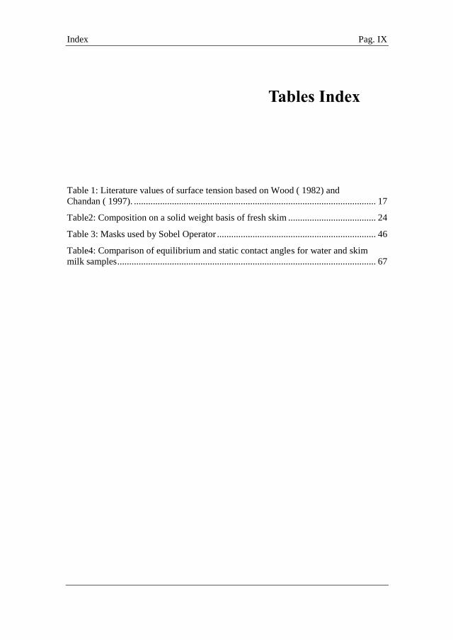
Tables Index

Table 1: Literature values of surface tension based on Wood ( 1982) and

Chandan ( 1997). ...................................................................................................... 17

Table2: Composition on a solid weight basis of fresh skim ..................................... 24

Table 3: Masks used by Sobel Operator ................................................................... 46

Table4: Comparison of equilibrium and static contact angles for water and skim

milk samples ............................................................................................................. 67

Pag. X Study of the Parameters affecting the coalescence Lara Ventura

[XI]

Sommario

Lo spray drying, essiccamento per nebulizzazione, è ampiamente

utilizzato in diversi settori industriali compreso quello alimentare,

farmaceutico e chimico. Si tratta di un processo unitario,in cui si ha la

trasformazione di un “liquidfeed” (soluzione, sospensione, emulsione)

in un particolato solido secco. Al fine di fare valutazioni sulla

dimensione finale della particella prodotta, risulta necessario

considerare la natura delle interazioni che si instaurano tra le

particelle, queste possono essere suddivise in interazioni: goccia-

goccia, goccia-particella e particella-particella.

Soffermandosi sulla prima tipologia e dunque sull’interazione goccia-

goccia, incrementando le velocità relative delle due gocce collidenti, è

possibile distinguere i seguenti regimi: (i) rimbalzamento, (ii)

coalescenza permanente, (iii) separazione e (iv) frantumazione. La

nostra attenzione è focalizzata sulla coalescenza permanente,

fenomeno fisico che si verifica quando due gocce si uniscono per

darne una di entità maggiore.

Dunque al fine di capire la cinetica di coalescenza è analizzato il

comportamento di due gocce di latte scremato su una superficie

idrofobica, a temperatura ambiente, mediante un tensiometro ottico.

In particolare il lavoro si è concentrato sull’analisi della variazione di

tensione superficiale e dell’angolo di contatto dei campioni presi in

esame.

Seguendo le linee guida dell’ ADSA, analisi incentrata sul profilo

della goccia al fine di trarre informazioni utili quali la tensione

superficiale, le immagini delle due gocce sessili registrate tramite il

tensiometro ottico sono state analizzate.

Pag. XII Study of the Parameters affecting the coalescence Lara Ventura

Per poter estrarre gli angoli di contatto così come il profilo della

goccia, è utilizzato un codice sviluppato in Matlab, in grado di

costruire una curva Laplaciana, partendo dalla soluzione di un insieme

di equazioni differenziali non lineari, del primo ordine. L’obiettivo è

quello di produrre, variando alcuni parametri una curva in grado di

dare un “best fitting“ del profilo sperimentale della goccia.

Inoltre, è stato analizzato il meccanismo caratterizzante la coalescenza

di latte scremato concentrato, tramite freeze-drying, per poter seguire

l’evoluzione del processo con il tempo e capire in che modo il

contenuto d’acqua influisce sulla cinetica di coalescenza.

.

[XIII]

Abstract

Spray Drying is a widely applied process in several sectors, food,

pharmaceutical and chemical industries. It is a one-step processing

operation for transforming liquid feeds into dried powders. In order to

control powder formation during spray drying, it is important to

understand interactions between droplets/particles, such as droplet-

droplet, droplet-particle and particle-particle interactions.

These interactions are consequences of droplet/particle collisions and

they can lead to several regimes. Based on the level of increasing

relative speed during droplet/particle collisions, regimes can be

classified as: (i) bouncing, (ii) permanent coalescence, (iii) separation

(or grazing) and (iv) shattering.

This work is focused on studying the regime of permanent

coalescence of two single droplets. Coalescence is the process by

which primary droplets merge to form a second bigger droplet.The

aim of this work was to improve understanding of the coalescence-

kinetics of two single droplets of skim milk.

Coalescence-kinetics was explored using an optical tensiometer for

two droplets of skim milk at room temperature on a hydropobic

surface in terms of changes in surface tension and contact angle.

Using the optical tensiometer, contact mechanisms between two

sessile droplets were recorded and analyzed following the scheme of

ADSA, based on droplet shape analysis. Shapes and contact angles of

droplets were extracted by using a code implemented in MATLAB.

Sets of first-order, non-linear differential equations were solved to

find Laplacian curves, which matches surface profiles of droplets by

numerically integrating the Young-Laplace equation, thus providing

valuable information of the surface free energy of the system during

the coalescence process.

Pag. XIV Study of the Parameters affecting the coalescence Lara Ventura

Furthermore, droplets of skim milk with different water contents,

obtained by freeze-drying,were used to follow the evolution of

coalescence-kinetics as a function of time and water content.

[81]

Appendix

Pag. 82 Study of the parameters affecting the coalescence Ventura Lara

A.1 Contact Angle Analyzer

A.1.1 Implementation

1. Start.

Turn on the instrument and start program

Figure 60: Theta control program

2. Experimental Setup

Click the icon inherent to the experiment, in this case:Contact

Angle Experiment

Selectthe typology of Solid and Liquid (Heavy Phase)

Then, click Start

Figure 61: The Experimental Setup Window

Conclusions Pag. 83

3. Image Recording

Figure 62: The Image Recorder captures the measurement data

Lift or lower the sample stage until the solid is visible on the

bottom part of the screen.

Locate the needle on the center and at the top of the screen

Select a Record Mode, Normal/Fast/ Fast + Normal

To adjust the focus of the image turn the camera lens focus

adjustment until the image is focused.

Click Adjust Camera Setting to get appropriate intensity (green

on Focusing window)

Approach the needle to the sample stage to create the drop

Click Record and wait for the images to be recorded and press

Done

Figure 63: Adjust Camera Settings


4. Curve fitting

Figure 64 : The Curve fitting window

Click Calibrate with the Needle, since the diameter of needle

0.71 mm is known

Check visually the position of the BaseLine and set it manually

by clicking and dragging on the white circle. Place the blue

box around the entire drop profile and press Execute.

5. Data Analysis

Figure 65: Conducted Measurements are analyzed in the Browse Exps.

Conclusions Pag. 85

B.1 Program Code

%B.1.1 Extraction of frames

%Referencing to Matlab file “extractionframes.m”.

1. %This function is used in order to extract the frame from the

movie of coalescence.

2. % Clear and close all opened materials

3. close all

4. clear all 5. % selection of the frames to analyze

6. for k=1:1029

7. % reading of the movie and storing the frame in a new variable

8. obj1=mmreader('14movie.avi');

9. fig=read(obj1,k);

10. % show the frame

11. I=imshow(fig);

12. % save the extracted frame specifying the name and the format

of the new image

13. saveas(I,sprintf('coalescence14.%d.jpg',k));

14. end


%B.1.2 Movie analysis

1. %The function used to analyze the movie is movieanalysis.m, in

detail to the milk at 95% of water content.

2. close all

3. clear all

4. measuringangle=input('typology of angle:1-right,2-left:');%

Choose the typology of angle

5. for r=272:1029 %number of frames

6. [valueapex,height,angle,angle1,angle2]=evaluation(r,measuringa

ngle)% recall the function evaluation.m

7. end 8. %export data from txt to excel

9. load('ellipse.txt')%ellipse data

10. if measuringangle==1

11. load('dataright.txt'); % load the data concerning the right angle

inMatlab

12. Headers={'rangle','dropheight','apexvalue'};% vector containing

a text string

13. % Import the results in excel

14. xlswrite('95%milkright',Headers,1,'A1');

15. xlswrite('95%milkright',dataright(:,1),1,'A3');

16. xlswrite('95%milkright',dataright(:,2),1,'B3');

17. xlswrite('95%milkright',dataright(:,3),1,'C3');

18. winopen('95%milkright.xls')% open the excel window to the

user

19. xlswrite('95%milkellipse',ellipse(:,1),1,'A3');

20. xlswrite('95%milkellipse',ellipse(:,2),1,'B3');

21. elseif measuringangle==2% other condition true for left angle

22. load('dataleft.txt');

23. Headers={'langle','dropheight','apexvalue'};

24. xlswrite('95%milkleft',Headers,1,'A1');

25. xlswrite('95%milkleft',dataleft(:,1),1,'A3');

26. xlswrite('95%milkleft',dataleft(:,2),1,'B3');

27. xlswrite('95%milkleft',dataleft(:,3),1,'C3');

28. winopen('95%milkleft.xls')

29. xlswrite('95%milkellipse',ellipse(:,1),1,'C3');

30. xlswrite('95%milkellipse',ellipse(:,2),1,'D3');

31. end

Conclusions Pag. 87

%B.1.3 Determining the contact Angle on a Substrate

1. % The function evaluation.m is used in order to measure the

contact angle so as the height and the radius at the apex, of the

droplet.

2. % the input are r, the number of the frame analyzed and

measuring angle, a variable that defines the type of angle

analyzed, as output the measurement of angle and all the elements

needed to define the drop shape.

3. function[valueapex,heigth,angle,angle1,angle2]=evaluation(r,meas

uringangle)

4. %selection of the image stored in a new file named droplet

5. droplet=strcat('coalescence14.',num2str(r),'.jpg')

6. I=imread(droplet);% importation of the image of the droplet

7. I2=im2bw(I,0.5);% make black and white image

8. % Crop an area for the droplet

9. % is an automatic selection of the object of interest [x, y,w,h]

10. % define a rectangular area

11. rect=[200 300 600 200];

12. I2=imcrop(I2,rect);

13. % edge detection

14. BW1 = edge(I2,'sobel');

15. % identification of the droplet from the background

16. Acrop=BW1;

17. [m,n]=size(Acrop);

18. k=1;% initiaziling the variable k

19. for i=1:n

20. for j=1:m

21. if Acrop(j,i)==1

22. y(k)=j;

23. x(k)=i;

24. k=k+1;

25. end

26. end

27. end 28. % Recall the experimental data using new variables

29. a=size(y);% length of the vector y

30. b=a((2));

31. y_=y;

32. x_=x;

33. % Approximation of the droplet trough an ellipse


34. % construction of a vector of ten points starting from the left

boundary

35. w=1;% initializing variable used as index for the vector x_l

36. s=10;

37. for N =1:s

38. x_l(w)=x(N);% define as column vector x_l containing x

coordinates

39. y_l(w)=y(N);

40. w=w+1;

41. end 42. % construction of a vector of ten points starting from the right

boundary

43. e=size(x);

44. e=e(2);

45. f=(e-9);

46. q=1; % initializing of the variable used as index for the vector x_r

47. for N=f:e

48. x_r(q)=x(N);

49. y_r(q)=y(N);

50. q=q+1;

51. end 52. % a vector containing the twenty points is generated

53. t=size(x_r);

54. t=t(2);

55. x_st=zeros(1,s+t); %x_st vector containing the x coordinates for

the generation of the straightline

56. y_st=zeros(1,s+t);

57. m=1;

58. for i=1:s

59. x_st(m)=x_l(i);

60. y_st(m)=y_l(i);

61. m=m+1;

62. end 63. n=1;

64. for i=(s+1):(s+t)

65. x_st(i)=x_r(n);

66. y_st(i)=y_r(n);

67. end 68. % Fitting of the points trough a linear function, in order to find

the slope and the intercept

Conclusions Pag. 89

69. p=polyfit(x_st,y_st,1);

70. m=p(1);

71. q=p(2);

72. for i=1:b

73. y_st_1(i)=m.*x_(i)+q;

74. end 75. % Difference between the two functions, the straightline and the

experimental profile obtained from edge detection, in order to

clean the imperfections given from the detection.

76. fori=1:b

77. dati_y(i)=y_st_1(i)-y_(i);% difference between the y data

78. ifdati_y(i)>0% if the difference is greater than zero, the y

coordinate is equal to it

79. dati_ord(i)=dati_y(i);

80. else 81. dati_ord(i)=0;

82. end

83. end 84. % Store the new data, in order to obtain the correct drop profile

85. for i=1:b

86. y_(i)=dati_ord(i);

87. end 88. %Fitting of the experimental data with an ellipse

89. % choice of random parameters

90. alfa=120;

91. beta=100 ;

92. gamma=50 ;

93. psi=0 ;% eccentricity

94. clear parameters

95. clear err

96. % define the parameters to optimize the function

97. parameters=[alfa,beta,gamma,psi];

98. %Optimization

99. % multidimensional unconstrained non linear minimization, to

find the combination of parameters for which the function has a

minimum

100. [parameters,fval,exitflag,output]=fminsearch(@(parameters)

errorellipse(parameters,x_,y_),parameters);

101. [err]=errorellipse(parameters,x_,y_);% recall the function

errorellipse


102. ex(r)=exitflag; %to verify the iteration

103. output;

104. % The values of the parameters are replaced in the function

ellipseoptimal.m, in order to construct the ellipse, that gives a

best fitting of the experimental droplet

105. [yellipse,xellipse]=optimalellipse(parameters,x_,y_);

106. % intersection with axes

107. optparameters=parameters;

108. alfa=optparameters(1);% extraction of each parameter

109. beta=optparameters(2);

110. gamma=optparameters(3);

111. psi=optparameters(4);

112. x0=gamma-alfa*sqrt(1-(psi/beta)^2); % the intersection with

axis at the left of the droplet center

113. x1=gamma+alfa*sqrt(1-(psi/beta)^2); % intersection with axis

at the right of the center

114. % first estimate of the angles,evaluating those given from the

ellipse fitting

115. angle=acos((x0-gamma)/(alfa));

116. angle1=90-(angle*180)/(pi); % conversion in radians

117. clear angle

118. angle2=acos((x1-gamma)/(alfa));

119. angle2=90-(angle2*180)/(pi);

120. h=(psi+beta); %height of the droplet

121. fid=fopen('ellisse.txt','a'); %open the data file

122. fprintf(fid,' %6.2f %6.2f\n',angle1,angle2); %write the values

into the file

123. fclose(fid);

124. % Store the experimental data in other variables not to generate

confusion in Matlab

125. x_n=x;

126. y_n=y:

127. % Definition of the apex, starting from ellipse

128. apex_x=gamma;

129. apex_z=beta;

130. % Introduction to the core of the code, definition of all

parameters and steps needed to solve Laplace-Young equation

131. % Fluid properties

132. wc=0.95;%water content in this case

133. u=(wc/ (1-wc));

Conclusions Pag. 91

134. ds=1470;% kg/m^3;% solid density

135. dw=1000; %kg/m^3%water density

136. rho_m=((u+1)/(u/dw+1/ds))/10^3; %density of fluid, [g/cm^3]

137. rho_a=0.0012;%density of surround fluid,typically air

138. g=981.7;% gravity acceleration [cm/s^2]

139. sig=49.913222;% surface tension [dyne/cm] for milk at 95% of

wc

140. %Definition of c, capillarity constant in unit of 1/cm2

141. c=((rho_m-rho_a)*g)/sig;

142. %Conversion

143. %through ImageJ

144. %0.71mm(calibration for the needle of the tensiometer)=102.82

pixels

145. %change the coordinate in X and Z

146. %conversion to cm and replacement of x with X and of y with Z

147. Xi=x_n(:)*0.00069;

148. Zi=y_n(:)*0.00069;

149. % conversion for the apex

150. apex_x=apex_x*0.00069;

151. apex_z=apex_z*0.00069;

152. % Collocation of the origin in the apex origin

153. Xi_new=(-Xi+apex_x)*c^0.5;

154. Zi_new=(-Zi+apex_z)*c^0.5;

155. %conversion for x0 e x1

156. x0=x0*0.00069;

157. x1=x1*0.00069;

158. x0=(-x0+apex_x)*c^0.5;

159. x1=(-x1+apex_x)*c^0.5;

160. % Selection of the positive data, for right angle

161. k=1;

162. a=size(Xi_new);


164. for i=1:a

165. if Xi_new(i)>=0 &Xi_new(i)<= x0% the data must be positive

and lower than x0, the intersection point

166. Xi_new_pos_1(k)=Xi_new(i);

167. Zi_new_pos_1(k)=Zi_new(i);

168. k=k+1;

169. end

170. end


171. elseif measuringangle==2% selection of data needed to define

the left angle

172. for i=1:a

173. if Xi_new(i)<=0 &Xi_new(i)>= x1

174. Xi_new_pos_3(k)=-Xi_new(i);

175. Zi_new_pos_3(k)=Zi_new(i);

176. k=k+1;

177. end

178. end

179. end 180. %condition true only for left angle

181. If measuringangle==2

182. lungh=length(Zi_new_pos_3);

183. k=lungh;

184. fori =1:lungh

185. Xi_new_pos_1(k)=Xi_new_pos_3(i);% store the coordinate, in

order not to introduce other variables for the following

functions

186. Zi_new_pos_1(k)=Zi_new_pos_3(i);

187. k=k-1;

188. end

189. end 190. % Defined the experimental points,b and c is possible to solve

the set of ordinary differential equation

191. clear err

192. b=0.1292*2; % apex of curvature of first tentative

193. [err]=errorlaplace(b,c,Zi_new_pos_1,Xi_new_pos_1);% err is

the output of the newfunctionerrorlaplace.m

194. %Optimization for Laplace

195. clear xopt

196. [xopt]=fminsearch(@errorrlaplace,b,[],c,Zi_new_pos_1,Xi_new

_pos_1); % search the b value that gives the minimum of the

error function

197. %optimal value of b now bb,solve Laplace

198. bb=xopt;

199. [ x_ly_1,z_ly_1,Phi_ly_1]

=optimalaplace(bb,c,Xi_new_pos_1;Zi_new_pos_1);

200. % evaluation again of the coordinates needed to construct the

theoretical profile, with the value of optimal b

201. % Plot the experimental profile and the theoretical one

Conclusions Pag. 93

202. linesize=3;

203. textsize=15;

204. plot(Xi_pos,Zi_pos,'b','LineWidth',linesize)%experimental data

205. hold on

206. plot(x_ly_1,z_ly_1,'g')%Laplace's data

207. set(gca,'YDir','reverse');% rotation of the graph

208. xlabel('value of x')

209. ylabel('value of z')

210. title('Fitting Drop')

211. hold off

212. % Output variables

213. rightangle=max(Phi_ly_1);% right angle[degrees]

214. height=max(z_ly_1);%height of the droplet [cm]

215. error=err;

216. valueapex=xopt;

217. %Import results into a txt.file


219. fid=fopen('dataright.txt','a'); %open the data file

220. fprintf(fid,' %6.4f %6.4f %6.4f\n',angle,heigth,valueapex);

%write theresults into the file

221. fclose(fid); %close the file

222. elseif measuringangle==2

223. fid=fopen('dataleft.txt','a'); %open the data file

224. fprintf(fid,' %6.4f %6.4f %6.4f\n',angle,heigth,valueapex);

%write the values into the file

225. fclose(fid);

226. end

227. end

%B.1.3.1 Fitting trough an ellipse

1. %The function considered is errorellipse.m

2. function[err]=errorellipse(parameters,x_,y_)

3. alfa=parameters(1);%parameters characterizing the ellipse,

defined in input

4. beta=parameters(2);

5. gamma=parameters(3);

6. psi=parameters(4);

7. %Knowing the parameters is possible to construct the ellipse

starting from experimental data

8. s=size(x_);


9. s=s(2);

10. for i =1:s

11. if (psi/beta)>1% to select only positive roots

12. y_ellipse(i)=0;

13. elseif (x_(i)>=(gamma-alfa*(sqrt(1-(psi/beta).^2)))

&&x_(i)<=(gamma+alfa*(sqrt(1-(psi/beta).^2))))

14. y_ellipse(i)=(beta*(sqrt(1-((x_(i)-gamma)/alfa).^2))+psi);%

definition of the ordinata for ellipse

15. else 16. y_ellipse(i)=0;

17. end

18. end 19. %Evaluation of the error,as the difference between the ordinata

of the two functions, the drop profile and ellipse

20. for i=1:s

21. res(i)=(y_(i)-y_ellipse(i)).^2;

22. end 23. %sum the errors

24. err=sum(res);

25. end

%B.1.3.2 Optimization ellipse

1. % Reference to the function optimalellipse.m, has been

constructed the ellipse with the optimal combination of

parameters

2. function[yellipse,xellipse]=optimalellipse(parameters,x_,y_)

3. alfa=parameters(1);

4. beta=parameters(2);

5. gamma=parameters(3);

6. psi=parameters(4);

7. s=size(x_);

8. s=s(2);

9. fori =1:s

10. if (psi/beta)>1

11. yellipse(i)=0;

12. elseif (x_(i)>= (gamma-alfa*(sqrt(1-(psi/beta).^2))) &&

x_(i)<=(gamma+alfa*(sqrt(1-(psi/beta).^2))))

13. yellipse(i)=(beta*(sqrt(1-((x_(i)-gamma)/alfa).^2))+psi);

14. else 15. yellipse(i)=0;

Conclusions Pag. 95

16. end 17. xellipse(i)=x_(i);end

%B.1.3.3 Laplace equation

1. % LAPLACE defines the ordinary differential equations to be

solved.

2. % z=drop height

3. % x=distance from axis to drop interface

4. % phi=contact angle

5. % 1/b=radius of curvature at apex

6. % s=arc length

7. % NON−DIMENSIONALIZE Z,X,S,B USING C^(1/2)

8. % B=b*c^(1/2)

9. % X=x*c^(1/2)

10. % Z=z*c^(1/2)

11. % S=s*c^(1/2)

12. %.No need to define X,Z,S for equations

13. % Z=y(1); Z'=dy(1); Z' is with respect to S

14. % X=y(2); X'=dy(2); X' is with respect to S

15. % phi=y(3); phi'=dy(3); phi' is with respect to S

16. % Z'=sin(phi)

17. % X'=cos(phi)

18. % phi'=2/B+Z−(sin(phi)/X)

19. function [dy]=laplace(s,y,b,c)

20. dy = zeros(3,1); % a column vector

21. B=b*c^.5; % non-dimensionalized curvature at apex

22. dy(1)=sin(y(3));

23. dy(2)=cos(y(3));

24. dy(3)=(2/B)+y(1)-(sin(y(3))/y(2));

25. end

%B.1.3.4 Error function for b

1. function[err]=errorlaplace(b,c,Zi_new_pos_1,Xi_new_pos_1)

2. S_span=(0:.001:1);%S_span is the step variable for ode45 solver

3. [S,Y]=ode45(@laplace,S_span,[0 1e-100 0],[],b,c);

4. x_ly(:,1)=Y(:,2);

5. z_ly(:,1)=Y(:,1);

6. S_ly(:,1)=S(:,1);

7. Phi_ly(:,1)=Y(:,3)*(180/pi);

8. k=1;


9. b=max(Zi_new_pos_1);

10. a=size(z_ly);

11. fori=1:a

12. ifz_ly(i)<b% selection of the points considering the maximum

of the experimental data

13. z_ly_1(k)=z_ly(i);

14. x_ly_1(k)=x_ly(i);

15. k=k+1;

16. end

17. end 18. f=size(x_ly_1);

19. f=f(2);

20. %Comparison between only selected points

21. primox=x_ly(1);

22. primoz=z_ly(1);

23. mediox=x_ly(round(f/2));

24. medioz=z_ly(round(f/2));

25. finalex=x_ly(f);

26. finalez=z_ly(f);

27. s=round(f/2);

28. secondox=x_ly(round(f-s/2));%from the basis to the middle

point

29. secondoz=z_ly(round(f-s/2));

30. %fifth point

31. quintox=x_ly(round(s/2));

32. quintoz=z_ly(round(s/2));

33. %sixth point

34. met=round(s/2);

35. sestox=x_ly(round(f-s/2));

36. sestoz=z_ly(round(f-s/2));

37. %seventh point

38. sett=round(met/2);

39. settimox=x_ly(round(f-sett/2));

40. settimoz=z_ly(round(f-sett/2));

41. %eight (chosen this value because is to close to the point of

interest)

42. ottavox=x_ly(f-22);

43. ottavoz=z_ly(f-22);

44. %selection the same points but using experimental data

45. d=size(Xi_new_pos_1);

Conclusions Pag. 97

46. d=d(2);

47. primox1=Xi_new_pos_1(d);

48. primoz1=Zi_new_pos_1(d);

49. mediox1=Xi_new_pos_1(round(d/2));

50. medioz1=Zi_new_pos_1(round(d/2));

51. finalex1=Xi_new_pos_1(1);

52. finalez1=Zi_new_pos_1(1);

53. e=round(d/2);

54. secondox1=Xi_new_pos_1(round(e/2));

55. secondoz1=Zi_new_pos_1(round(e/2));

56. %fifth point

57. quintox1=Xi_new_pos_1(round(d-e/2));

58. quintoz1=Zi_new_pos_1(round(d-e/2));

59. %sixth point

60. mes=round(e/2);

61. sestox1=Xi_new_pos_1(round(mes/2));

62. sestoz1=Zi_new_pos_1(round(mes/2));

63. setts=(mes/2);

64. settimox1=Xi_new_pos_1(round(setts/2));

65. settimoz1=Zi_new_pos_1(round(setts/2));

66. ottavox1=Xi_new_pos_1(22);

67. ottavoz1=Zi_new_pos_1(22);

68. %evaluation of error

69. xmax=Xi_new_pos_1(1);%define the maximum of data

70. %parameters that are important to define the error

71. eps=10^(-3);

72. a=1;

73. %error calculated as the distance between the experimental

point and the one obtained from Laplace,the error is weighted

74. res1=(0.5)*(1/((abs(primox1-xmax))â+eps))*((primox-

primox1)^2+(primoz-primoz1)^2);

75. res2=(0.5)*(1/((abs(mediox1-xmax))â+eps))*((mediox-

mediox1)^2+(medioz-medioz1)^2);

76. res3=(0.5)*(1/((abs(finalex1-xmax))â+eps))*((finalex-

finalex1)^2+(finalez-finalez1)^2);

77. res4=(0.5)*(1/((abs(secondox1-xmax))â+eps))*((secondox-

secondox1)^2+(secondoz-secondoz1)^2);

78. res5=(0.5)*(1/((abs(quintox1-xmax))â+eps))*((quintox-

quintox1)^2+(quintoz-quintoz1)^2);


79. res6=(0.5)*(1/((abs(sestox1-xmax))â+eps))*((sestox-

sestox1)^2+(sestoz-sestoz1)^2);

80. res7=(0.5)*(1/((abs(settimox1-xmax))â+eps))*((settimox-

settimox1)^2+(settimoz-settimoz1)^2);

81. res8=(0.5)*(1/((abs(ottavox1-xmax))â+eps))*((ottavox-

ottavox1)^2+(ottavoz-ottavoz1)^2);

82. err=(res1+res2+res3+res4+res5+res6+res7+res8)*1000;

83. end

%B.1.3.5 Optimization Laplace

1. %The function optimalaplace.m is used in order to construct

the theoretical profile starting with the optimal value of b

2. S_span=(0:.001:1);

3. [S,Y]=ode45(@laplace,S_span,[0 1e-100 0],[],bb,c);

4. x_ly(:,1)=Y(:,2);

5. z_ly(:,1)=Y(:,1);

6. S_ly(:,1)=S(:,1);

7. Phi_ly(:,1)=Y(:,3)*(180/pi);

8. k=1;

9. b=max(Zi_new_pos_1);

10. a=size(z_ly);

11. fori=1:a

12. ifz_ly(i)<b

13. Phi_ly_1(k)=Phi_ly(i);

14. z_ly_1(k)=z_ly(i);

15. x_ly_1(k)=x_ly(i);

16. k=k+1;

17. end

18. end

19. end

[99]

References

1. R.E.M. Verdurmen, M. Verschueren, J. Straatsma and M. Gunsing,

Simulation of agglomeration in spray drying installationsthe EDECAD

project,DOI: 10.1081/DRT-120038735 (2004)

2. By N. ASHGRIZ AND J. Y. POO, Coalescence and separation in binary

collisions ofliquid drops, J. Fluid Mech. (1990)

3. Melissa Orme, Experiments on droplet collisions, bounce, coalescence and

disruption, Elsevier Science PH:S0360

4. Adam, J.R., Lindblad, N.R. and Hendricks, C. D., The collision,

coalescence and disruption of water droplets. Journal of Applied Physics,

1968, 39(11), 5173-5180.

5. F. Mashayek, N. Ashgriz, W.J. Minkowycz, B.Shotorban, Coalescence

collision of liquid drops, International Journal of Heat and Mass Transfer

46(2002)77-89

6. R.Narhe, D.Beysens and V.S. Nikolayev, Contact Line Dynamics in Drop

Coalescence and Spreading, Langmuir2004,20,1213-1221

7. C.Andrieu, D. A. Beysens, V.S. Nikolayev and Y. Pomeau, Coalescence of

sessile drops, J. Fluid Mech.(2002), vol.453, pp.427-438

8. J.Drelich, R.Zahn, J.D. Miller and J.K. Borchardt, 2002 Contact angle

relaxation for ethoxylated alcohol solutions on hydrophobic surfaces,

Contact Angle Wettability, and Adhesion, Vol. 2, pp. 253-264

9. C.H. Whitnah, The Surface Tension Of Milk, 1959 American Dairy

Science Association. Published by Elsevier Inc.

10. Chandan, R. Dairy Based Ingredients: Practical Guides for the Food

Industry, Eagen Press Handbook Series, USA, 1997.

11. Wood, P.W. Physical Properties of Dairy Products, Ministry of Agriculture

and Fisheries (MAF), New Zealand, 1982.

12. Niloshree Mukherjee, Bipan Bansal, Xiao Dong Chen, Measurement of

Surface Tension of Homogenised Milks, International Journal of Food

Engineering, Volume 1, Issue 2 (2005)


13. Yuehua Yuan and T.Randall Lee, Contact Angle and Wetting Properties,

Springer, Heidelberg 2013

14. Roger P. Woodward, Ph.D., Surface Tension Measurements Using The

Drop Shape Method, First Ten Angstroms, 2008

15. F. Bashforth, J.C. Adams, An Attempt to Test the Theory of Capillary

Action (Cambridge, London, 1892).

16. Richard M. Bidwell, J. L. Duran, Jr. Grant L. Hubbard, Tables For The

Determination of the surface tensions of liquid metals by the pendant drop

method, University of California Los Alamos Scientific Laboratory Los

Alamos, New Mexico, August 28 1964

17. C.N. Catherine Lam, James J.Lu and A.Wilhelm Neumann, Measuring

Contact Angle, Analysis and Characterization in Surface Chemistry

18. O.I. del Rìo, A. W. Neumann,Axisymmetric Drop Shape Analysis:

Computational Methods for the Measurement of Interfacial Properties from

the Shape and Dimensions of Pendant and Sessile Drops, J. Colloid

Interface Sci. 196, 136(1997)

19. P. Cheng, D. Li, L. Boruvka, Y.Rotenberg, A.W. Neumann, Colloids Surf.

43, 151(1990)

20. Sabine Ullrich, Quantitative Measurements of Shrinkage and Cracking

during freeze-drying of amorphous cakes, A theysis, 26 June (2014)

21. Antoine Diana, Martin Castillo, David Brutin, Ted Steinberg, Sessile Drop

Wettability in Normal and Reduced Gravity, Microgravity Sci. Technol.,

07 January 2012

22. Aurélien F. Stalder, Tobias Melchior, Michael Muller, Daniel Sage,

Thierry Blu, Michael Unser, Low-bond axisymmetric drop shape analysis

for surface tension and contact angle measurements of sessile drops,

Colloids Surf. A: Physicochem. Eng.Aspects (2010)

23. Thomas Young, An Essay on the Cohesion of Fluids, 1 January (1805)

24. Russell Stacy, Contact Angle Measurement Technique for Rough Surfaces,

A Thesis, 2009

25. VinaykumarKonduru, A Thesis, Static and Dynamic Contact Angle

Measurement on Rough Surfaces Using Sessile Drop Profile Analysis with

Application to Water Management in Low Temperature Fuel Cells,

Michigan Technological University 2010.

26. Ken Osborne, A Thesis, Determining the Contact Angle of a Droplet on a

Substrate, Worcester Polytechnic Institute, March 2008

27. C Atae-Allah et al., Measurement of surface tension and contact angle

using entropic edge detection, Measurement Science and Technology

28. ElhamJasim Mohammad et al., Study Sobel Edge Detection Effect on The

Image Edges Using Matlab, International Journal of Innovative Research in

Science, Engineering and Technology, vol.3, Issue 3, March 2014

References Pag. 101

29. G.T. Shrivakshan, Dr. C. Chandrasekar, A Comparison of various Edge

Detection Techniques used in Image Processing, IJCSI International

Journal of Computer Science Issues, Vol. 9, Issue 5, No 1, September 2012

30. Aldo Handojo, YumeiZhai, Gerald Frankel, Melvin A. Pascall,

Measurement of adhesion strengths between various milk products on

glass surfaces using contact angle measurement and atomic force

microscopy, Journal of Food Enginnering 92(2009)


Acknowledgements

I am grateful to Prof. Gaetano Lamberti, for his big patience and

support, he has been a lighthouse for me during this thesis

work.

I am deeply grateful to Prof. Lilia Ahrnè, for giving me the

possibility to make a new experience and to work with her

research group.

I would like to express my gratitude to my co-supervisor during the

project , Dr. Loredana Malafronte, for her help, suggestions

and all the encouragements, she has been a friendly co-

supervisor.

My sincere thanks go to all the people of the Department of Process

and Technology Development of SP and to the entire group of

Transport Phenomena & Processes at University of Salerno, in

particular to Diego Caccavo, for the daily little helps.

I want to thank my family for believing in me, a particular thanks

goes to my uncle: I always feel his presence in the daily little

good things that happen to me.

I wish to express my gratitude to my fellow students at UNISA, for

their big support.

Special thanks also to my Erasmus friends, we have spent

unforgettable moments together.

Salerno 18/09/2015 Lara Ventura

Date post:	05-Apr-2018
Category:	Documents
Upload:	vunhi
View:	219 times
Download:	3 times

Experimental Study of the parameters affecting the...

Documents