Experimental study of the properties of the Higgs boson · The various Higgs boson production and...

Experimental study of theproperties of the Higgs boson

Richard David Mudd

Thesis submitted for the degree ofDoctor of Philosophy

Particle Physics Group,School of Physics and Astronomy,University of Birmingham.

January 25, 2016

University of Birmingham Research Archive

e-theses repository This unpublished thesis/dissertation is copyright of the author and/or third parties. The intellectual property rights of the author or third parties in respect of this work are as defined by The Copyright Designs and Patents Act 1988 or as modified by any successor legislation. Any use made of information contained in this thesis/dissertation must be in accordance with that legislation and must be properly acknowledged. Further distribution or reproduction in any format is prohibited without the permission of the copyright holder.

Abstract

Measurements of Higgs boson production and decay rates are presented using theproton-proton collision data collected by the ATLAS experiment during LHC Run I,corresponding to 4.5 fb−1 at

√s = 7 TeV and 20.3 fb−1 at

√s = 8 TeV. Under certain

assumptions, the coupling strengths of the Higgs boson to Standard Model particlesare also probed.

The H → ZZ(∗) → 4` final state, where ` = e, µ, is discussed in detail, and isobserved with a significance corresponding to 8.1 standard deviations. The Higgsboson production rate, relative to the Standard Model prediction, is measured to beµ = 1.44+0.40

−0.33 at the ATLAS best-fit value for the measurement of the Higgs bosonmass, mH = 125.36 GeV. Grouping similar Higgs boson production modes, theproduction rates relative to the SM prediction for the fermionic production modes -gluon fusion and associated production with a tt or bb pair - and bosonic productionmodes - vector boson fusion and associated production with a W or Z boson - aremeasured to be µggF+ttH+bbH = 1.7+0.5

−0.4 and µV BF+V H = 0.3+1.6−0.9, respectively.

The various Higgs boson production and decay modes studied by the ATLAS ex-periment are also combined, where the measured overall Higgs boson rate, relativeto the Standard Model prediction, is 1.18+0.15

−0.14. The couplings of the Higgs bosonare probed in a number of benchmark models, where a good agreement with theStandard Model prediction is observed for each model considered. The Higgs bosoncoupling measurements are also used to place constraints on a number of beyond theStandard Model theories, and are combined with direct searches for invisible Higgsboson decays to place a limit on the Higgs boson branching ratio to invisible finalstates.

i

Declaration of author’s contribution

The design and construction of the ATLAS experiment, as well as the LHC, rep-resents the significant efforts of large number individuals over many years. EveryATLAS result, including those presented in this thesis, owe a significant debt tothese efforts.

The remarkably successful operation of the ATLAS detector during the first run ofthe LHC, again due to the work of many people, has underpinned the entire physicsprogramme, and I have been fortunate to have had the opportunity to contributeto this in an operational role during 2012.

Offline performance studies also play a big role in facilitating physics results, and tothis end I have contributed to the Level-1 Calorimeter Trigger efficiency monitoringand the development of trigger algorithms used during the 2012 8 TeV run. Ialso performed a detailed study of the application of isolation criteria to electrontriggers at the hardware level, work that was subsequently continued by severalother collaborators and underpins the ability of ATLAS to trigger events containingW± and Z bosons in LHC Run II. This work is not described in this thesis, thoughseveral aspects are described in approved ATLAS internal documents [1, 2].

This thesis focuses on the Higgs sector, and in particular the experimental study ofthe coupling properties of the observed Higgs boson. Chapters 4, 5 and 6 summarisethe results that I have contributed to in this area.

Chapters 4 and 5 document the ATLAS H → ZZ(∗) → 4` analysis, where I havecontributed to all ATLAS publications [3, 4, 5] and preliminary results [6] sinceSummer 2012. With several collaborators, I developed, maintained and ran analysissoftware to perform the full analysis. Though a baseline event selection for theinclusive analysis had already been defined when I started my work on this analysis,

ii

iii

I participated in the optimisation of the analysis, and in particular in the definitionof production based categories to enable a measurement of the signal strengths ofthe various Higgs boson production modes. I have also contributed extensivelyto the data-driven background estimation, the modelling of signal and backgrounddistributions, the final statistical interpretation of results, the Higgs boson massmeasurement [7] and the search for high mass resonances.

I have also been involved in the first search for Higgs boson decays to a quarkoniumstate plus a photon, primarily in the signal and background modelling and statisticalinterpretation. This work is not discussed in this thesis, and is described in Ref. [8].

I have been involved in the combination of Higgs boson decay modes and the sub-sequent rate and couplings measurements [9]. In particular I have performed thecorrelation of systematic uncertainties across different final states and performedmaximum likelihood fits in a number of models, described in this thesis. This in-cludes the combination of off-shell and on-shell analyses, and the combination ofvisible and invisible decay modes. I have also used the coupling measurements tostudy directly several beyond the Standard Model scenarios [10].

Finally, I have contributed to the overall LHC - ATLAS and CMS - Higgs bosoncouplings combination [11] as the ATLAS contact for the H → ZZ(∗) → 4` channel.

Acknowledgements

Reflecting on four years that have seemed to pass very quickly, I am somewhatoverwhelmed by the extent and nature of the support I have received from a greatmany sources. It is, of course, impossible to suitably acknowledge every individual,group and organisation to whom I am grateful. Below are some scattered thoughts,but it should be emphasised that I am truly appreciative of everyone who has playeda part, large or small, in making the work described in this thesis possible.

Firstly, I gratefully acknowledge the financial support that I have received from theSTFC and the University of Birmingham. The opportunity to work day-to-day onsomething that is simultaneously stimulating, challenging and enjoyable is rare, andthis would not have been possible for me if not for this generous support.

I owe a great debt to my Ph.D. supervisors, whose guidance has been invaluable.Kostas Nikolopoulos is a remarkable physicist and person. I am thankful for hispatience, his unwavering support, his advice (not always taken but always wise)and friendship. More than this, Kostas has always endeavoured to be professional,principled and empathetic and has taught me lessons reaching far beyond ParticlePhysics. I would also like to express my gratitude to Paul Newman and JurajBracinik. Paul’s faith in me and enthusiasm for particle physics were key factorsin bringing me to Birmingham, and I greatly appreciate the advice and support hehas consistently provided since I have been here. Working with Juraj has also beenan immense pleasure; he is one of the most positive, friendly and helpful people I’veever met, and helped me immensely as a newcomer to the ATLAS collaboration.

It has been my great privilege to collaborate with, learn from, and get to know manyPhysicists from across the world and I appreciate the many stimulating discussionsI have had with members of the ATLAS collaboration. I am grateful in particularto colleagues from the working groups that I have been a part of. I am thankful to

iv

v

the ATLAS Level-1 Trigger community for the friendly, welcoming and supportiveenvironment I experienced in the early parts of my Ph.D. I am also grateful tothe ATLAS Higgs boson working group, in particular the H → ZZ(∗) sub-group.I thank the sub-group convenors and paper editors I have had the opportunity towork closely with - Christos Anastopoulos, Stefano Rosati, Fabien Tarrade, RosyNikolaidou, Robert Harrington, Roberto Di Nardo and R.D. Schaffer - for theirsupport and guidance.

I also thank Eleni Mountricha for her collaboration and patience in the early parts ofmy Ph.D., and Tim Adye for expert technical guidance and the many hours spenthelping me. I am thankful to all of my colleagues in the particle physics groupat the University of Birmingham, in particular the Birmingham ATLAS group, forthe support, guidance and stimulating discussions. It has been a real privilege tohave had the opportunity to work closely with my friends Andy Chisholm, LudovicaAperio Bella and Paul Thompson.

The company of fellow Ph.D. students has contributed immensely to making thepast four years an enjoyable and memorable experience. For this, I am grateful tomy fellow University of Birmingham students and especially those in West 316 -Tim, Jody, Tom, Hardeep, Benedict, Andy C (again), Andrew, “Mi Amigo” Javier,Mark, Rhys, Matt, James, Andy F and Alasdair. Thanks for the Friday beers, thecurries, the football and the drinks at the Belgian Bar; I had fun.

I am fortunate to have had the opportunity to spend an extended period at CERN,though this would have been very difficult if it were not for the company of themany great friends I met there, in particular those residing at Citadines in Ferney-Voltaire, especially Carl, Shaun, Gary, Sam, Nikki, “The Ravens”, Jim and Craig(and everyone I’ve forgotten to mention). I will remember fondly the pool parties,the kebabs and, again, the drinks at the Belgian Bar.

I am grateful to my friends outside of academia, whose support, encouragement andinterest has been a great motivation. I would also like to express my gratitude to myextended family, especially my grandparents and great-grandparents. This includesthe Evanses, in particular Chris and Stan, who have warmly welcomed me into theirfamily.

Most importantly, I am indebted to those closest to me. I am grateful to my parents,Jane and Steve, and my Brother, Andrew: thank you, for your love and uncondi-tional support, for always believing in me, and for so much more. You have alwaysinspired me. Finally, I am grateful to Sammy: thank you for everything and more.You’ve shared this experience with me and it hasn’t always been easy - I appreciatethe sacrifices that you’ve made and the support and love you’ve shown me morethan I can possibly express. I couldn’t imagine spending these (and the rest of my)years with anyone else.

This thesis is dedicated to my Mum and Dad, to Andrew, and to Sammy.

vi

All I know is that I don’t know nothing... and that’s fine.

Operation Ivy, “Knowledge”

Contents

1 Introduction 1

2 The Higgs boson 42.1 The Higgs boson and the Standard Model . . . . . . . . . . . . . . . . 4

2.1.1 Electroweak theory . . . . . . . . . . . . . . . . . . . . . . . . . 72.1.2 The Brout-Englert-Higgs (BEH) mechanism . . . . . . . . . . . . . 72.1.3 Alternative and extended Higgs sectors . . . . . . . . . . . . . . . 9

2.2 SM Higgs boson production and decay at the LHC . . . . . . . . . . . . 122.3 Measurement of the Higgs boson rates and probing its couplings . . . . . 162.4 Simulation . . . . . . . . . . . . . . . . . . . . . . . . . . . . . . . . . 20

2.4.1 Higgs boson signal simulation . . . . . . . . . . . . . . . . . . . . 212.4.2 Background simulation for H → ZZ(∗) → 4` . . . . . . . . . . . . 22

3 The ATLAS experiment at the LHC 243.1 The LHC . . . . . . . . . . . . . . . . . . . . . . . . . . . . . . . . . . 243.2 The ATLAS detector . . . . . . . . . . . . . . . . . . . . . . . . . . . . 26

3.2.1 Coordinate system and quantity definitions . . . . . . . . . . . . . 273.2.2 Magnet system . . . . . . . . . . . . . . . . . . . . . . . . . . . 283.2.3 Inner detector . . . . . . . . . . . . . . . . . . . . . . . . . . . . 293.2.4 Calorimeters . . . . . . . . . . . . . . . . . . . . . . . . . . . . 313.2.5 Muon spectrometer . . . . . . . . . . . . . . . . . . . . . . . . . 353.2.6 Trigger and data acquisition . . . . . . . . . . . . . . . . . . . . . 36

3.3 Data Sample . . . . . . . . . . . . . . . . . . . . . . . . . . . . . . . . 393.3.1 Luminosity Measurement . . . . . . . . . . . . . . . . . . . . . . 42

3.4 Physics object reconstruction and identification . . . . . . . . . . . . . . 433.4.1 Muons . . . . . . . . . . . . . . . . . . . . . . . . . . . . . . . 433.4.2 Electrons . . . . . . . . . . . . . . . . . . . . . . . . . . . . . . 463.4.3 Photons . . . . . . . . . . . . . . . . . . . . . . . . . . . . . . . 513.4.4 Jets . . . . . . . . . . . . . . . . . . . . . . . . . . . . . . . . . 51

4 H → ZZ(∗) → 4` with the ATLAS detector 534.1 Event selection . . . . . . . . . . . . . . . . . . . . . . . . . . . . . . . 544.2 Higgs boson reconstruction . . . . . . . . . . . . . . . . . . . . . . . . 57

4.2.1 Final state radiation recovery . . . . . . . . . . . . . . . . . . . . 574.2.2 Z-Mass Constraint . . . . . . . . . . . . . . . . . . . . . . . . . 59

4.3 Discrimination against SM diboson production . . . . . . . . . . . . . . 604.4 Background estimation . . . . . . . . . . . . . . . . . . . . . . . . . . . 63

vii

CONTENTS viii

4.4.1 Estimate of the ``µµ background . . . . . . . . . . . . . . . . . . 664.4.2 Estimate of the `èe background . . . . . . . . . . . . . . . . . . 72

4.4.2.1 The 3`+X method . . . . . . . . . . . . . . . . . . . . 734.4.2.2 The transfer factors method . . . . . . . . . . . . . . . . . 764.4.2.3 The reco-truth unfolding method . . . . . . . . . . . . . . . 77

4.4.3 Background control plots . . . . . . . . . . . . . . . . . . . . . . 784.5 Signal and background modelling . . . . . . . . . . . . . . . . . . . . . 80

4.5.1 Signal modelling . . . . . . . . . . . . . . . . . . . . . . . . . . 804.5.2 Background modelling . . . . . . . . . . . . . . . . . . . . . . . . 814.5.3 Likelihood function . . . . . . . . . . . . . . . . . . . . . . . . . 84

4.6 Systematic Uncertainties . . . . . . . . . . . . . . . . . . . . . . . . . . 854.7 Results . . . . . . . . . . . . . . . . . . . . . . . . . . . . . . . . . . . 87

4.7.1 Higgs boson mass and inclusive signal strength measurement . . . . . 954.7.1.1 ATLAS combined measurement . . . . . . . . . . . . . . . 954.7.1.2 Combined ATLAS and CMS measurement . . . . . . . . . . 98

4.7.2 Fiducial and differential cross section measurements . . . . . . . . . 101

5 Higgs boson production rates and couplings in the H → ZZ(∗) → 4`channel 1035.1 Event categorisation . . . . . . . . . . . . . . . . . . . . . . . . . . . . 103

5.1.1 VBF enriched category selection criteria . . . . . . . . . . . . . . . 1055.1.1.1 Boosted Decision Tree classifier for VBF enriched category . . . 105

5.1.2 VH-hadronic enriched category selection criteria . . . . . . . . . . . 1085.1.2.1 Boosted Decision Tree classifier for VH-hadronic enriched category109

5.1.3 VH-leptonic enriched category selection criteria . . . . . . . . . . . 1115.1.4 Expected yields . . . . . . . . . . . . . . . . . . . . . . . . . . . 112

5.2 Background estimation in categories . . . . . . . . . . . . . . . . . . . . 1125.3 Categorisation-specific systematic uncertainties . . . . . . . . . . . . . . 1145.4 Modelling and statistical treatment . . . . . . . . . . . . . . . . . . . . 1155.5 Results . . . . . . . . . . . . . . . . . . . . . . . . . . . . . . . . . . . 1195.6 Prospects for future measurements of production and decay rates in the

H → ZZ(∗) → 4` final state . . . . . . . . . . . . . . . . . . . . . . . . 1275.6.1 Up to 100 fb−1 at 13 TeV . . . . . . . . . . . . . . . . . . . . . . 1275.6.2 Up to 3000 fb−1 with an upgraded, HL-LHC . . . . . . . . . . . . . 129

6 Higgs boson production and decay rates and couplings using thecombination of decay modes 1346.1 Input channels to the combination . . . . . . . . . . . . . . . . . . . . . 1356.2 Combination procedure . . . . . . . . . . . . . . . . . . . . . . . . . . 1426.3 Production and decay rates . . . . . . . . . . . . . . . . . . . . . . . . 1436.4 Coupling strength measurements . . . . . . . . . . . . . . . . . . . . . 146

6.4.1 Fermion versus vector coupling strengths . . . . . . . . . . . . . . 1486.4.2 Fermion coupling sector . . . . . . . . . . . . . . . . . . . . . . . 1506.4.3 Beyond the SM contributions . . . . . . . . . . . . . . . . . . . . 151

6.4.3.1 Direct searches for Higgs boson decays to invisible final states . 1536.4.4 Generic Models . . . . . . . . . . . . . . . . . . . . . . . . . . . 155

ix CONTENTS

6.4.4.1 Generic Model 1 . . . . . . . . . . . . . . . . . . . . . . 1556.4.4.2 Generic Model 2 . . . . . . . . . . . . . . . . . . . . . . 157

6.4.5 Constraints on the Higgs boson invisible branching ratio combining

visible and invisible decay modes . . . . . . . . . . . . . . . . . . . 1606.5 Constraints on new phenomena using Higgs boson coupling measurements163

6.5.1 Minimal Composite Higgs Models . . . . . . . . . . . . . . . . . . 1636.5.2 Additional EW Singlet Model . . . . . . . . . . . . . . . . . . . . 164

7 Concluding remarks 168

CHAPTER 1

Introduction

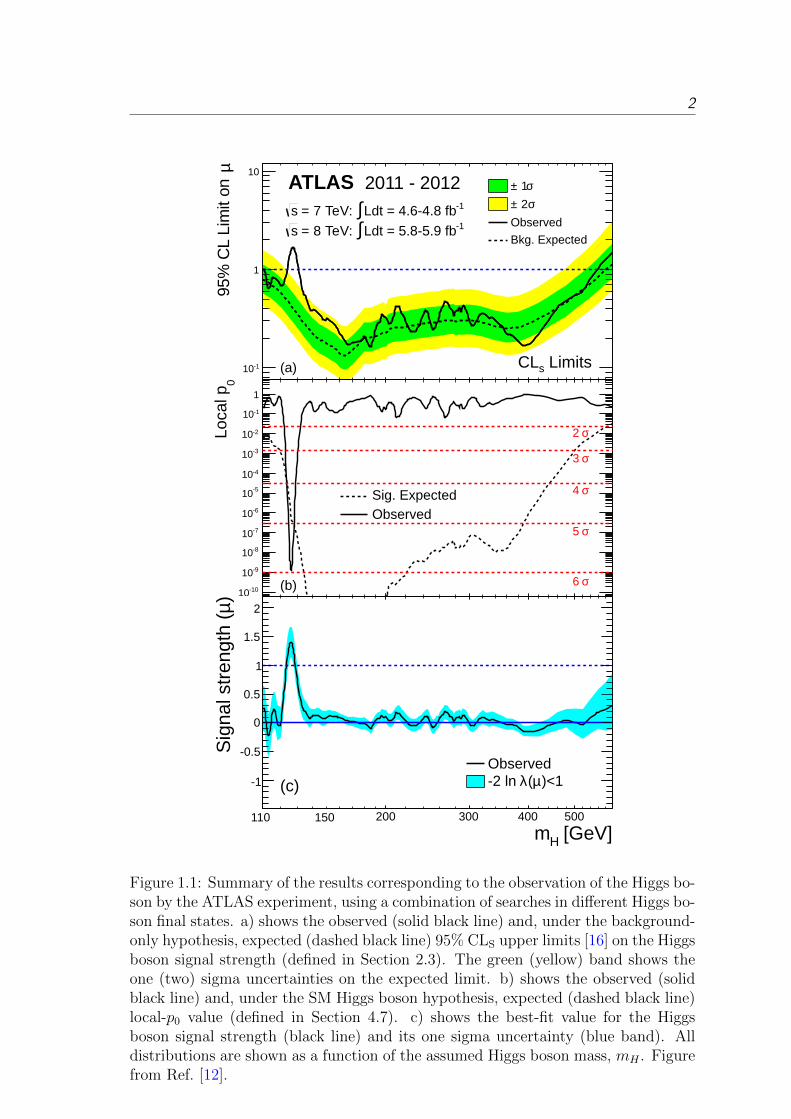
In July 2012, the ATLAS and CMS collaborations reported the discovery of a Higgs

boson with a mass, mH , around 125 GeV [12, 13], representing the culmination of

many years of searches at a number of experimental facilities, with notable recent

examples being at LEP [14] and the Tevatron [15]. A summary of the ATLAS

results is shown in Figure 1.1. Many subsequent analyses have been performed to

test the compatibility of the observed boson’s properties with those predicted by

the Standard Model, some of which form the main part of this document.

Chapter 2 gives an overview of some of the relevant theoretical background, as

well as the expected phenomenology of the SM Higgs sector and the details of

theoretical calculations and simulations. Chapter 3 contains a brief description of

the Large Hadron Collider and the ATLAS experiment, including details about the

reconstruction of physics objects and the data sample used for analyses contained

in this thesis.

1

2

200 300 400 500

µ95

% C

L Li

mit

on

-110

1

10

σ 1±σ 2±

Observed

Bkg. Expected

ATLAS 2011 - 2012-1Ldt = 4.6-4.8 fb∫ = 7 TeV: s -1Ldt = 5.8-5.9 fb∫ = 8 TeV: s

LimitssCL(a)

0Lo

cal p

-1010

-910

-810

-710

-610

-510

-410

-310

-210

-110

1

Sig. ExpectedObserved

(b)

σ2

σ3

σ4

σ5

σ6

[GeV]Hm200 300 400 500

)µS

igna

l str

engt

h (

-1

-0.5

0

0.5

1

1.5

2

Observed)<1µ(λ-2 ln (c)

110 150

Figure 1.1: Summary of the results corresponding to the observation of the Higgs bo-son by the ATLAS experiment, using a combination of searches in different Higgs bo-son final states. a) shows the observed (solid black line) and, under the background-only hypothesis, expected (dashed black line) 95% CLS upper limits [16] on the Higgsboson signal strength (defined in Section 2.3). The green (yellow) band shows theone (two) sigma uncertainties on the expected limit. b) shows the observed (solidblack line) and, under the SM Higgs boson hypothesis, expected (dashed black line)local-p0 value (defined in Section 4.7). c) shows the best-fit value for the Higgsboson signal strength (black line) and its one sigma uncertainty (blue band). Alldistributions are shown as a function of the assumed Higgs boson mass, mH . Figurefrom Ref. [12].

3 CHAPTER 1. INTRODUCTION

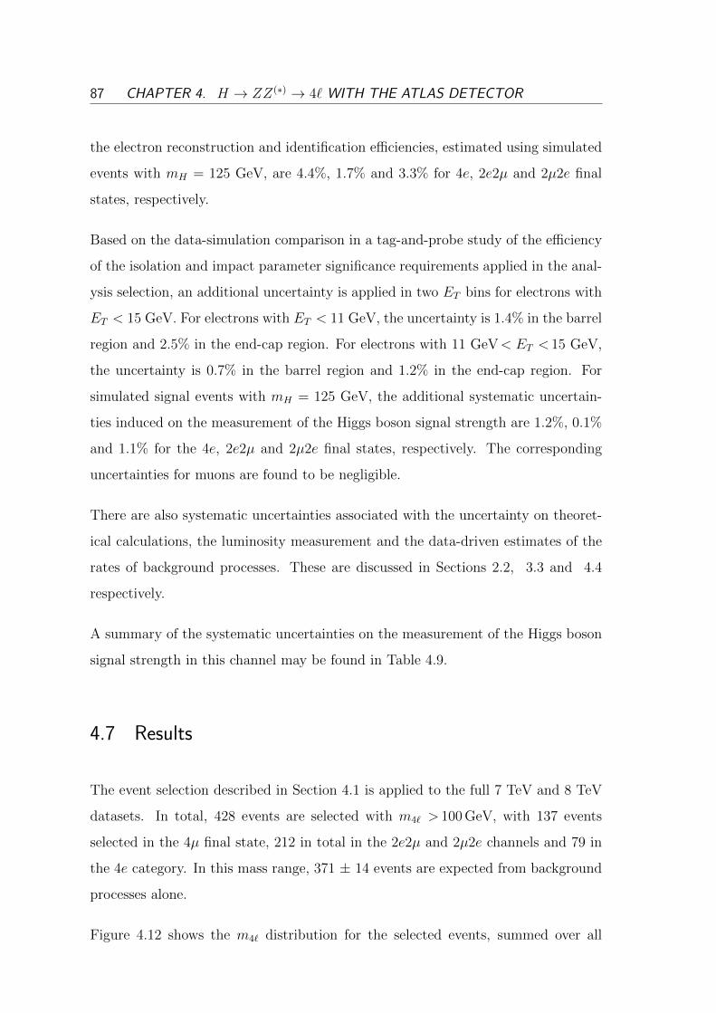
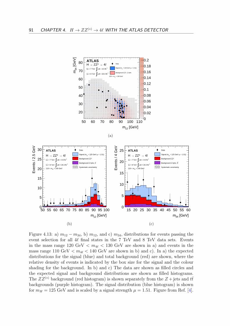
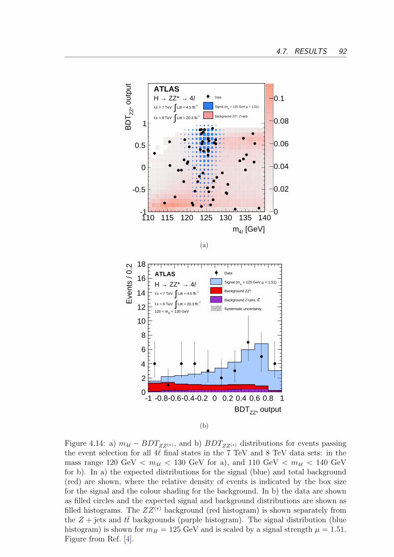
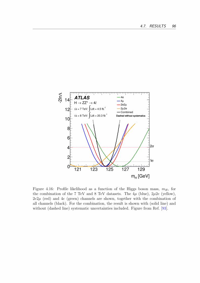
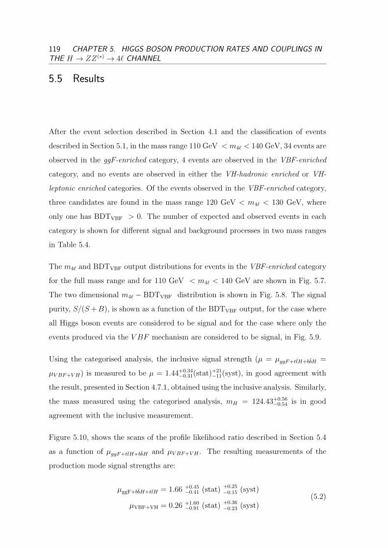
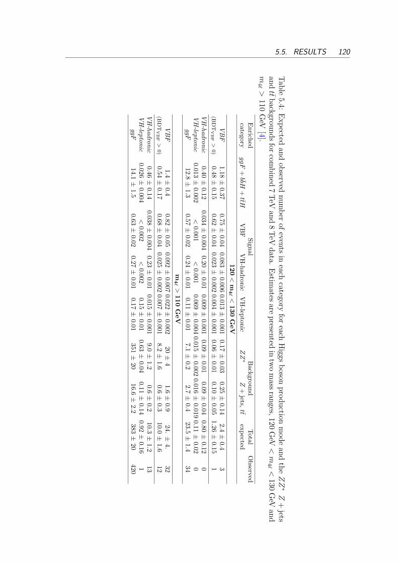
Chapters 4 and 5 discuss the ATLAS H → ZZ(∗) → 4` analysis:

- Chapter 4 details the so-called “inclusive analysis” and the subsequent mea-

surements of the Higgs boson mass, inclusive signal strength and differential

cross sections.

- Chapter 4 focuses in detail on the “categorised analysis” used to measure the

signal strengths for different Higgs boson production modes and extract the

Higgs boson couplings.

Chapter 6 focuses on the measurement of the Higgs boson production and decay rates

using the combination of the various decay modes and the subsequent extraction of

the Higgs boson couplings. Direct constraints placed on “beyond the Standard

Model” theories using the coupling measurements are also discussed.

Finally, Chapter 7 closes the thesis with some concluding remarks.

CHAPTER 2

The Higgs boson

2.1 The Higgs boson and the Standard Model

In modern elementary particle physics, the current best understanding of the fun-

damental constituents of matter and their interactions is provided by the Stan-

dard Model (SM) [17, 18]. The SM, whose interactions are derived by imposing

SU(3)C ⊗ SU(2)L ⊗ SU(1)Y local gauge symmetry, describes constituent fermions,

classified into families of quarks and leptons, that are assumed to be point like

and whose interactions are mediated by the strong, weak and electromagnetic (EM)

forces. Each force is associated with one or more gauge boson.

The quarks - up(u), down(d), charm(c), strange(s), top(t) and bottom(b) - and lep-

tons - electrons(e), muons(µ), taus(τ) and electron, muon and tau neutrinos(νe/µ/τ )

- are summarised in Table 2.1. The gauge bosons associated with the strong force

and EM force are the gluon(g) and photon(γ) respectively and both are mass-

4

5 CHAPTER 2. THE HIGGS BOSON

less. Three massive gauge bosons are associated with the weak force, the neu-

tral Z boson (mZ = 91.1876 ± 0.0021 GeV), and the charged W+ and W− bosons

(mW± = 80.385± 0.015 GeV) [19].

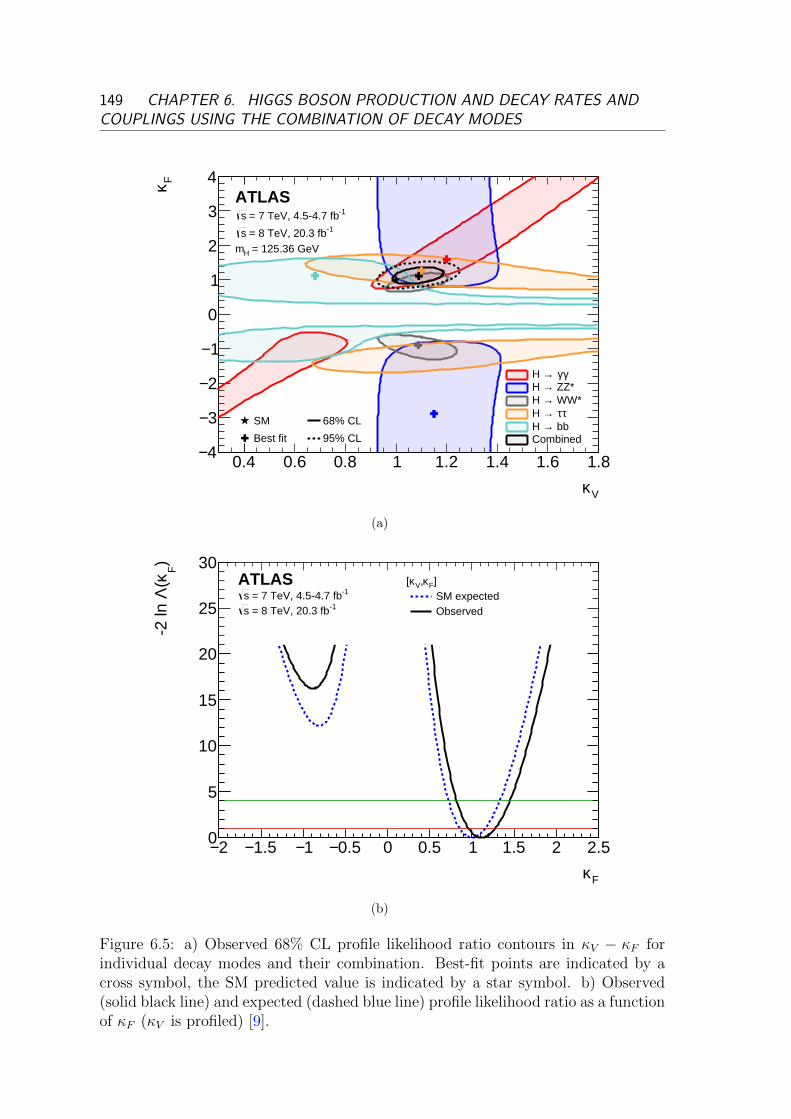
The SU(2)L⊗SU(1)Y symmetry provides a unified description of the EM and weak

forces in a single Quantum Field Theory, despite their significant phenomenological

differences, and is discussed in Section 2.1.1. The SU(3) symmetry corresponds

to Quantum Chromodynamics (QCD), a non-abelian gauge theory describing the

strong interaction.

Quarks and leptons are distinguished by the fact that quarks carry colour charge,

whereas leptons do not; thus QCD acts only on the quark sector and is mediated

by gauge bosons known as gluons. Unlike photons in Quantum Electrodynamics

(QED) that do not carry electric charge, gluons do carry a colour charge and as a

consequence self-interact. Only states with net-zero colour are observed in isolation,

so quarks, anti-quarks and gluons appear in colour-neutral bound states known as

hadrons. Up, down, charm, strange and bottom quarks all become part of bound

states, a process known as hadronisation, though top quarks decay too quickly to

hadronise.

In scattering experiments final state partons are typically observed as part of col-

limated bunches of hadrons known as jets. However, a jet is not uniquely defined,

and typically an algorithm must be defined to associate constituent particles with

a particular jet. Finally, since the Large Hadron Collider (LHC), described in Sec-

tion 3.1, is a proton-proton (p − p) collider, the initial state particles are hadrons

and hard collisions in fact occur between the proton constituents. As a consequence,

parton distribution functions are required to describe the distribution of quarks and

gluons within the protons.

2.1. THE HIGGS BOSON AND THE STANDARD MODEL 6

Tab

le2.1:

Mass

and

electricch

arge(in

units

ofth

eelectron

charge)

forth

eth

reefam

iliesof

fermion

sin

the

SM

.M

assvalu

es,estim

atedusin

gth

eM

Ssch

eme

excep

tfor

the

topquark

mass

(where

adirect

measu

remen

tis

quoted

),are

takenfrom

Ref.

[19].In

general,

the

uncertain

tieson

the

lepton

masses

arecon

siderab

lysm

allerth

anth

euncertain

tieson

the

quark

masses.

Neu

trinos

arecon

sidered

massless

inth

eSM

.

Genera

tion

III

IIIQ

uark

sSym

bol

ud

cs

tb

Mass

4.8+

0.7

−0.5

MeV

2.3+

0.7

−0.5

MeV

1.275±

0.025G

eV95±

5M

eV173.21

±0.51±

0.71G

eV4.18±

0.03G

eVE

lectricC

harge

+2/3

-1/3+

2/3-1/3

+2/3

-1/3L

epto

ns

Sym

bol

eνe

µνµ

τντ

Mass

0.511000

105.65M

eV0

1776.8M

eV0

Electric

Charge

-10

-10

-10


2.1.1 Electroweak theory

Guided by the observed phenomenology, the theory of EW interactions is based on

the SU(2)L ⊗ SU(1)Y gauge group. The physical fermions are made up of left-

handed and right-handed fields; the left-handed components transform as doublets

under SU(2), whereas the right-handed components transform as singlets, so the

weak interaction only acts on the left-handed components.

The requirement for the theory to be invariant under local gauge transformations,

leads to a weak isovector Wµ, corresponding to SU(2) with coupling constant g, and

a weak isoscalar Bµ, corresponding to U(1) with a coupling constant g′. At odds

with experimental observations, this model alone requires both the vector bosons

and the fermions to be massless since Dirac mass terms do not respect the local

gauge invariance of the symmetry group.

2.1.2 The Brout-Englert-Higgs (BEH) mechanism

In the SM, the Brout-Englert-Higgs (BEH) mechanism generates masses for the

vector bosons and fermions [20, 21, 22]. A complex, self-interacting SU(2) scalar

doublet, labelled the Higgs doublet, is introduced:

φ =

φ+

φ0

with a potential, shown in Figure 2.1, given by:

V (φ) = µ2φ†φ+λ2

2(φ†φ)2

where choosing µ2 < 0 results in the neutral component of the doublet acquiring

a non-zero vacuum expectation value, v =√

2µ/λ ' 246 GeV. Since the ground

state of φ is degenerate and is not symmetric under local SU(2)L ⊗ SU(1)Y gauge

transformations, the symmetry is said to be spontaneously broken.


)φIm

(

)φRe(

)φV

(

Figure 2.1: The Higgs potential, V (φ).

Three of the four SU(2)L ⊗ SU(1)Y generators are spontaneously broken, leading

to the existence of three massless Goldstone bosons, associated with three of the

four degrees of freedom introduced by the Higgs doublet. The Higgs field couples

to the Wµ and Bµ gauge fields through the kinetic term of the Higgs Lagrangian,

and as a result the three degrees of freedom associated with the Goldstone bosons

become the longitudinal polarisation components of the physical W and Z bosons.

The fourth generator is unbroken, and corresponds to U(1)EM , which means the

photon remains massless. The remaining degree of freedom introduced by the scalar

doublet corresponds to the Higgs boson itself.

After the introduction of the Higgs field, Yukawa interactions between the Higgs

boson and the SM fermions can be added to the SM Lagrangian. When the Higgs

field acquires a vacuum expectation value as described above, the Yukawa interaction

terms generate fermion masses.

The Higgs boson itself is a massive, scalar boson, whose mass is mH =√

2λv,


where v is the vacuum expectation value of the Higgs field and λ, the Higgs self

coupling parameter, is a free parameter in the SM. The Higgs boson mass is hence

not predicted by the SM.

For a given value of the Higgs boson mass, its couplings to SM particles are predicted,

and depend linearly on the fermion mass for Higgs boson-fermion couplings, gHff ,

and on the boson mass squared for Higgs boson-vector boson couplings, gHV V :

gHff =mf

v, gHV V =

2m2V

v

A further motivation for the introduction of a BEH mechanism is the preservation

of unitarity in the W+W− → W+W− process, where without a Higgs boson, the

scattering amplitude for the process rises at a faster rate than the total cross section.

After introducing the Higgs boson, unitarity is recovered due to a series of new

processes (including a Higgs boson exchange) with the same initial and final states.

2.1.3 Alternative and extended Higgs sectors

The tree level Higgs boson mass is subject to radiative loop corrections due to

heavy particles, in the SM dominated by the top quark and with further significant

contributions from the W and Z bosons. Such loop processes are required to be

calculated up to a scale determined by the domain of the validity of the SM which, in

the absence of heavy new physics, is considered to be the Planck scale, O (1019) GeV.

In this case, for a physical Higgs boson mass at the electroweak scale, the stability of

the Higgs boson mass is provided by a high degree of parameter fine-tuning. Several

extended or alternative models for EWSB have been proposed to construct theories

that are able to avoid this problem, and are also able to explain the source of EWSB.

In Composite Higgs Models (CHM), the Higgs boson is not a fundamental

scalar but a composite, pseudo Nambu-Goldstone boson, associated with the spon-

taneous breaking of a global “flavour” symmetry in a strongly interacting sector.


EWSB is generated dynamically by loop processes involving SM bosons and fermions

and radiative corrections to the Higgs boson mass are saturated at a so-called com-

positeness scale, so the mass remains low even in the presence of heavy new physics.

For Minimal Composite Higgs Models (MCHM), interactions are derived by

imposing SO(5) gauge symmetry, and the Higgs boson couplings to vector bosons

take the form:

gHV V = gSMHV V ·√

1− ξ

where ξ = v2/f 2 is a scale factor that depends on the compositness scale, f , and the

SM vacuum expectation value, v. The form of the Higgs boson couplings to fermions

depends on the chosen representation for fermions in the theory, and two variants of

MCHM are correspondingly defined: MCHM4 [23], where spinorial representations

of SO(5) are chosen, and MCHM5 [24, 25], where fundamental representations of

SO(5) are chosen. The fermion couplings for each variant take the following form:

gHff = gSMHff ·√

1− ξ(MCHM4)

gHff = gSMHff ·1− 2ξ√

1− ξ(MCHM5)

The SM predictions are recovered in the limit ξ = 0.

A central prediction of the BEH mechanism is:

ρ = M2W / (M2

Z · cos2θW ) = 1 (2.1)

at tree level, where θW is the Weinberg angle. This parameter has been precisely

measured at LEP [26]. Choosing suitable quantum numbers, this is also the case

in models with additional Higgs multiplets. Several models extend the scalar sector

with the introduction of further fields. In Additional Electroweak Singlet Mod-

els, a single, real field, transforming as a singlet under SU(3)C ⊗SU(2)L⊗SU(1)Y ,

is added to the theory [27, 28]. Both the Higgs field and the singlet field acquire


a non-zero vacuum expectation value, and the singlet state mixes with the original

Higgs doublet, with the additional degree of freedom introduced giving rise to a

second scalar boson.

The lighter and heavier bosons are denoted as h and H respectively, and the cou-

plings of each to vector bosons and fermions are modified by a factor κ2 (for h) and

κ′2 (for H). For this Higgs sector to unitarise W+W− → W+W− scattering it is

required that κ2 + κ′2 = 1. Assuming SM decays modes, the branching ratios of

the lighter state are identical to those in the SM, and the branching ratios of the

heavy state are modified with respect to the SM predictions to take into account

new kinematically accessible decay modes (including final states containing h). The

transformation properties of the EW singlet under the SU(3)C ⊗ SU(2)L⊗ SU(1)Y

gauge symmetry mean that this model provides a dark matter candidate.

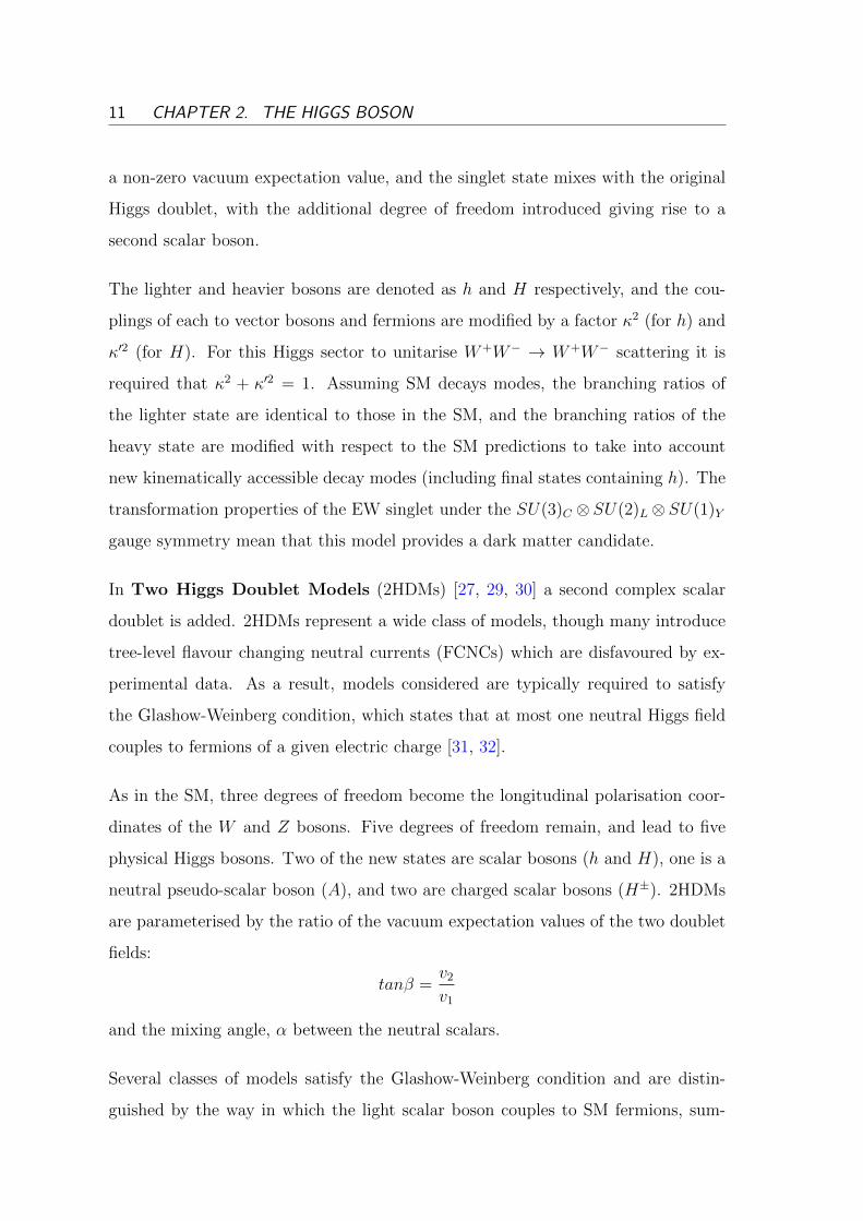
In Two Higgs Doublet Models (2HDMs) [27, 29, 30] a second complex scalar

doublet is added. 2HDMs represent a wide class of models, though many introduce

tree-level flavour changing neutral currents (FCNCs) which are disfavoured by ex-

perimental data. As a result, models considered are typically required to satisfy

the Glashow-Weinberg condition, which states that at most one neutral Higgs field

couples to fermions of a given electric charge [31, 32].

As in the SM, three degrees of freedom become the longitudinal polarisation coor-

dinates of the W and Z bosons. Five degrees of freedom remain, and lead to five

physical Higgs bosons. Two of the new states are scalar bosons (h and H), one is a

neutral pseudo-scalar boson (A), and two are charged scalar bosons (H±). 2HDMs

are parameterised by the ratio of the vacuum expectation values of the two doublet

fields:

tanβ =v2

v1

and the mixing angle, α between the neutral scalars.

Several classes of models satisfy the Glashow-Weinberg condition and are distin-

guished by the way in which the light scalar boson couples to SM fermions, sum-

2.2. SM HIGGS BOSON PRODUCTION AND DECAY AT THE LHC 12

marised in Table 2.2. The Minimal Supersymmetric Standard model is an example

of a 2HDM.

Table 2.2: Coupling scale factors, κV , κu, κd and κ`, that scale the SM Higgsboson coupling to vector bosons, up-type quarks, down-type quarks and leptonsrespectively in several classes of 2HDM [10].

Coupling scale Type I Type II Type III Type IVfactorκV sin(β − α) sin(β − α) sin(β − α) sin(β − α)κu cos(α)/ sin(β) cos(α)/ sin(β) cos(α)/ sin(β) cos(α)/ sin(β)κd cos(α)/ sin(β) − sin(α)/ cos(β) cos(α)/ sin(β) − sin(α)/ cos(β)κl cos(α)/ sin(β) − sin(α)/ cos(β) − sin(α)/ cos(β) cos(α)/ sin(β)

2.2 SM Higgs boson production and decay at the LHC

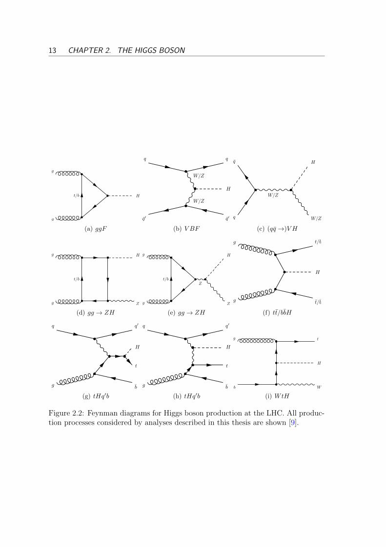
Several Higgs boson production modes are relevant at the LHC. The Feynman dia-

grams for the Higgs boson production mechanisms considered by analyses discussed

in this thesis are shown in figure 2.2.

The cross sections for Higgs boson production processes and their associated uncer-

tainties are compiled in Refs. [33, 34]. The Higgs boson gluon fusion (ggF ) cross

section has been calculated to next-to-leading order (NLO) [35, 36, 37] and next-to-

next-to-leading order (NNLO) [38, 39, 40] in QCD. QCD soft-gluon resummations

to the Higgs boson ggF cross section have been calculated in the next-to-next-

to-leading log (NNLL) approximation [41]. Finally, NLO EW corrections are also

applied [42, 43]. The Vector Boson Fusion (VBF) process is calculated with full

NLO QCD and EW corrections [44, 45, 46]. Approximate NNLO QCD corrections

are applied [47]. For the processes where the Higgs boson is produced in associa-

tion with a vector boson (WH/ZH), calculations are performed at NLO [48] and

NNLO [49] in QCD, and EW radiative corrections [50] are calculated to NLO. For

the process where the Higgs boson is produced in association with a pair of top

quarks (ttH), the cross section is calculated to NLO in QCD [51, 52, 53, 54].

Assuming a Higgs boson mass mH = 125 GeV, the QCD scale uncertainty for the


t/b

g

g

H

(a) ggF

W/Z

W/Z

q′

q

q′

q

H

(b) V BF

W/Z

q

q

W/Z

H

(c) (qq →)V H

t/b

g

g

Z

H

(d) gg → ZH

t/bZ

g

g

Z

H

(e) gg → ZH

g

g

t/b

t/b

H

(f) tt/bbH

g

q

b

q′

t

H

(g) tHq′b

g

q

b

q′

t

H

(h) tHq′b

b

g

W

H

t

(i) WtH

Figure 2.2: Feynman diagrams for Higgs boson production at the LHC. All produc-tion processes considered by analyses described in this thesis are shown [9].

2.2. SM HIGGS BOSON PRODUCTION AND DECAY AT THE LHC 14

ggF process is +7−8%, and the corresponding uncertainty for the V BF and V H pro-

duction processes is 1%. The production cross section uncertainty due to uncertain-

ties in the parton distribution function (PDF) and αs are ±8% for gluon-initiated

processes and ±4% for quark-initiated processes, estimated using the method de-

scribed in Ref [55] with the cteq [56], mstw [57] and nnpdf [58] PDF sets.

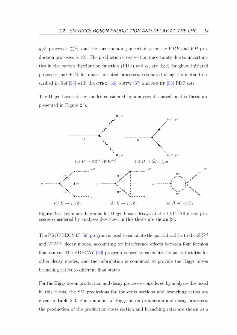
The Higgs boson decay modes considered by analyses discussed in this thesis are

presented in Figure 2.3.

H

W,Z

W,Z

(a) H → ZZ(∗)/WW (∗)

H

b, τ+, µ+

b, τ−, µ−

(b) H → bb/ττ/µµ

t/b

t/b

t/b

H

γ

γ/Z

(c) H → γγ/Zγ

W±

W−

W+

H

γ

γ/Z

(d) H → γγ/Zγ

W±

W±

H

γ

γ/Z

(e) H → γγ/Zγ

Figure 2.3: Feynman diagrams for Higgs boson decays at the LHC. All decay pro-cesses considered by analyses described in this thesis are shown [9].

The PROPHECY4F [59] program is used to calculate the partial widths to the ZZ(∗)

and WW (∗) decay modes, accounting for interference effects between four fermion

final states. The HDECAY [60] program is used to calculate the partial widths for

other decay modes, and the information is combined to provide the Higgs boson

branching ratios to different final states.

For the Higgs boson production and decay processes considered by analyses discussed

in this thesis, the SM predictions for the cross sections and branching ratios are

given in Table 2.3. For a number of Higgs boson production and decay processes,

the production of the production cross section and branching ratio are shown as a


function of the Higgs boson mass in Figure 2.4.

[GeV]H

M

100 150 200 250

BR

[p

b]

× σ

-410

-310

-210

-110

1

10

LH

C H

IGG

S X

S W

G 2

01

2

= 8TeVs

µl = e,

τν,µν,eν = νq = udscb

bbν± l→WH

bb-l+ l→ZH

b ttb→ttH

-τ+τ →VBF H

-τ+τ

γγ

qqν± l→WW

ν-lν

+ l→WW

qq-l+ l→ZZ

νν-l+ l→ZZ

-l

+l

-l

+ l→ZZ

Figure 2.4: SM prediction for Higgs boson production cross section times branchingratio as a function of the Higgs boson mass for a number of processes [33].

The Higgs boson width, assuming mH = 125 GeV, is ΓH = 4.15 MeV, far beyond

the experimental precision that a collider experiment could feasibly achieve. Recent

studies have observed that a sizeable cross section for the off-shell production of

a Higgs boson in the H → ZZ(∗) and H → WW (∗) decay modes may be observ-

able, and under certain assumptions the combination of the on-shell and off-shell

measurements may be used to indirectly constrain the Higgs boson width.

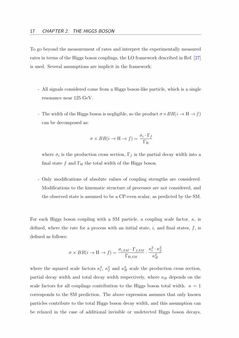
2.3. MEASUREMENT OF THE HIGGS BOSON RATES AND PROBING ITSCOUPLINGS 16

Table 2.3: SM predictions for Higgs boson production cross sections and decaysbranching ratios, along with their uncertainties, from Ref. [27] except for the tHproduction cross section, from Ref. [61]. The calculations assume a Higgs bosonmass mH=125 GeV.

Production Cross section (pb)

process√s = 7 TeV

√s = 8 TeV

ggF 15.0± 1.6 19.2± 2.0VBF 1.22± 0.03 1.57± 0.04WH 0.573± 0.016 0.698± 0.018ZH 0.332± 0.013 0.412± 0.013bbH 0.155± 0.021 0.202± 0.028ttH 0.086± 0.009 0.128± 0.014tH 0.012± 0.001 0.018± 0.001

Total 17.4± 1.6 22.3± 2.0

Decay channel Branching ratio (%)H → bb 57.1± 1.9H → WW ∗ 22.0± 0.9H → γγ 8.53± 0.85H → ττ 6.26± 0.35H → cc 2.88± 0.35H → ZZ∗ 2.73± 0.11H → γγ 0.228± 0.011H → Zγ 0.157± 0.014H → µµ 0.022± 0.001

2.3 Measurement of the Higgs boson rates and probing its

couplings

Measured rates in Higgs boson analyses are presented in terms of the signal strength

parameter µ, defined for a given decay mode as:

µ =σ · BR

σSM · BRSM

(2.2)

where σ is the total cross section of the Higgs boson and BR is the branching ratio

for the relevant mode. For specific production modes, this may be factorised as:

µ = µi · µf (2.3)

where µi = σi/σi,SM and µf = BRf/BRf,SM for a given production mode i and decay

mode f . Since only the product µi · µf is experimentally measured, measurements

of production or decay related quantites are required to make assumptions on µf or

µi respectively.


To go beyond the measurement of rates and interpret the experimentally measured

rates in terms of the Higgs boson couplings, the LO framework described in Ref. [27]

is used. Several assumptions are implicit in the framework:

- All signals considered come from a Higgs boson-like particle, which is a single

resonance near 125 GeV.

- The width of the Higgs boson is negligible, so the product σ×BR(i → H→ f )

can be decomposed as:

σ ×BR(i→ H→ f) =σi · Γf

ΓH

where σi is the production cross section, Γf is the partial decay width into a

final state f and ΓH the total width of the Higgs boson.

- Only modifications of absolute values of coupling strengths are considered.

Modifications to the kinematic structure of processes are not considered, and

the observed state is assumed to be a CP-even scalar, as predicted by the SM.

For each Higgs boson coupling with a SM particle, a coupling scale factor, κ, is

defined, where the rate for a process with an initial state, i, and final states, f , is

defined as follows:

σ ×BR(i→ H→ f) =σi,SM · Γf,SM

ΓH,SM

·κ2i · κ2

f

κ2H

where the squared scale factors κ2i , κ

2f and κ2

H scale the production cross section,

partial decay width and total decay width respectively, where κH depends on the

scale factors for all couplings contribution to the Higgs boson total width. κ = 1

corresponds to the SM prediction. The above expression assumes that only known

particles contribute to the total Higgs boson decay width, and this assumption can

be relaxed in the case of additional invisible or undetected Higgs boson decays,

2.3. MEASUREMENT OF THE HIGGS BOSON RATES AND PROBING ITSCOUPLINGS 18

where the Higgs boson total width becomes:

ΓH =κ2H

1− BRi.,u.

ΓH,SM

For the production and decay process considered by analyses discussed in this thesis,

the corresponding signal strength, written in terms of the coupling scale factors, is

shown in Table 2.4.

If the particle content of loops is assumed to be the same an in the SM, the loop

processes are resolved in terms of fundamental coupling scale factors as shown in

Table 2.4. To allow for the presence of additional, unknown particles running in

loops, effective coupling scale factors, κg, κγ and κZγ, are introduced in some fits

to scale the gg → H, H → γγ and H → Zγ processes. The gg → ZH process is

always resolved in terms of the SM predicted loop content as any deviation from the

SM is likely to give rise to a kinematic structure very different to the SM prediction.

Since each measured rate depends on the Higgs boson total width, which cannot be

measured directly at the LHC, only measurements of ratios of coupling scale factors

can be made without some assumption about the Higgs boson total width.

To measure absolute coupling scale factors, several possible assumptions can be

made to constrain ΓH :

- The Higgs boson does not decay to any additional invisible or undetected final

states, i.e. BRi.,u. = 0.

- The scale factors for the ZH and WH couplings do not exceed one, i.e. κW ≤ 1

and κZ ≤ 1. This is motivated by the assumption that the existence of the

Higgs boson solves the unitarity problem in vector boson scattering, and holds

in many BSM models [27].

- Under the assumption that the equivalent coupling strengths for off-shell Higgs

boson and on-shell Higgs boson production are identical, a measurement of the


Table 2.4: Higgs boson rate scalings in terms of coupling strength scale factors for theproduction and decay processes considered and the Higgs boson total width. Loopprocesses may depend on more than one coupling scale factor, and may includeinterference terms. The expressions are taken from Ref. [27], except for σ(gg →ZH), which is from Ref. [62], and σ(gb → WtH) and σ(qb → tHq′), which iscalculated using Ref. [61].

Production Loops Interference Rate scaling in terms of coupling scale factorsσ(ggF) X b− t κ

2g ∼ 1.06 · κ2

t + 0.01 · κ2b − 0.07 · κtκb

σ(VBF) - - ∼ 0.74 · κ2W + 0.26 · κ2

Z

σ(WH) - - ∼ κ2W

σ(qq → ZH) - - ∼ κ2Z

σ(gg → ZH) X Z − t κ2ggZH ∼ 2.27 · κ2

Z + 0.37 · κ2t − 1.64 · κZκt

σ(bbH) - - ∼ κ2b

σ(ttH) - - ∼ κ2t

σ(gb→ WtH) - W − t ∼ 1.84 · κ2t + 1.57 · κ2

W − 2.41 · κtκW

σ(qb→ tHq′) - W − t ∼ 3.4 · κ2t + 3.56 · κ2

W − 5.96 · κtκW

Partial decay widthΓbb - - ∼ κ

2b

ΓWW - - ∼ κ2W

ΓZZ - - ∼ κ2Z

Γττ - - ∼ κ2τ

Γµµ - - ∼ κ2µ

Γγγ X W − t κ2γ∼ 1.59 · κ2

W + 0.07 · κ2t − 0.66 · κWκt

ΓZγ X W − t κ2Zγ∼ 1.12 · κ2

W + 0.00035 · κ2t − 0.12 · κWκt

Total decay width

ΓH XW − tb− t κ

2H ∼

0.57 · κ2b + 0.22 · κ2

W + 0.09 · κ2g+

0.06 · κ2τ

+ 0.03 · κ2Z + 0.03 · κ2

c+

0.0023 · κ2γ

+ 0.0016 · κ2Zγ

+ 0.00022 · κ2µ

2.4. SIMULATION 20

off-shell Higgs boson production rate can be used to constrain the Higgs boson

total width.

- If it is assumed that the Higgs boson does not decay to additional undetected

final states, BRundet. = 0, then a direct limit on Higgs boson decays to invisible

final states can be used to constrain the Higgs boson total width.

As well as making measurements where each fundamental coupling is assigned a

scale factor (and variations upon this discussed so far), benchmark models with

reduced numbers of coupling scale factors may be probed. The benchmark models

considered are discussed alongside the obtained results in Section 5.5.

2.4 Simulation

The simulation of p − p collisions and the response of the ATLAS detector1 plays

a vital role in the analysis of data collected by the ATLAS experiment. A range

of event generator programs, using Monte Carlo (MC) simulation to model the

acceptance of events, are used to model the signal and background processes for

various analyses. Event generators are used to simulate the p − p interaction and

the subsequent decays, as well as the parton shower, hadronisation and underlying

event processes. In practice, the program used to simulate the hard interaction and

the program used to simulate the other processes may be different; in this case, the

latter is known as a ‘showering program’. Parton distribution functions (PDFs) are

used to parameterise the distribution of constituents inside the proton.

The collection of stable particles produced in the event generation process is inter-

faced to the ATLAS detector simulation, which uses the GEANT4 [63, 64] framework

to simulate the interaction of particles passing through a detailed model of the AT-

LAS detector geometry and material composition. The simulation of further p − p

interactions in the same bunch crossing is performed by superimposing the detector

1The ATLAS detector is described in Chapter 3.


activity from simulated minimum bias events.

2.4.1 Higgs boson signal simulation

For the ggF and V BF Higgs boson production modes, the hard scatter process is

modelled using the Powheg event generator program [65, 66, 67, 68, 69], which

uses next-to-leading order (NLO) matrix-element calculations. Pythia8 [70, 71] is

used as a showering program. For the WH and ZH processes, Pythia8 is used to

simulate both the hard scatter and the parton shower at leading-order (LO). For

the H → ZZ(∗) → 4` channel, discussed in detail in this thesis, the ttH process is

also simulated with Pythia8, whereas analyses specifically searching for ttH pro-

duction, described in Chapter 6, use Powheg for the hard scatter and Pythia8 for

showering. The bbH process is assumed to have the same acceptance and efficiency

as the ggF process as the event kinematics are found to be similar, and the same

Higgs boson mass dependence as the ttH process. The CT10 [72] and CTEQ6L1 [73]

PDF sets are used. Table 2.5 summarises the event generators and PDF sets used

for the main Higgs boson production modes.

Table 2.5: Summary of the event generators and PDF sets used to simulate Higgsboson production in

√s = 8 TeV p − p collisions, for the main production modes

considered [9].

Production Event Showering PDFprocess generator program set

ggF Powheg Pythia8 CT10VBF Powheg Pythia8 CT10WH Pythia8 Pythia8 CTEQ6L1ZH : qq → ZH Pythia8 Pythia8 CTEQ6L1ZH : gg → ZH Powheg Pythia8 CT10ttH Powheg Pythia8 CT10

The simulated samples are scaled to match the best available theoretical predictions

for the production cross sections and decay branching ratios for each process, taken

from Refs. [33, 34].

2.4. SIMULATION 22

For the ggF production mechanism, the generated Higgs boson pT distribution is

reweighted to match the calculations from Refs. [74, 75]. The calculation includes

NNLO and NNLL QCD corrections.

For the H → ZZ(∗) → 4` channel, discussed in detail in this thesis, the production

cross sections for various production modes and H → ZZ(∗) → 4` branching ratio is

presented for a series of Higgs boson mass values at 7 TeV and 8 TeV in Table 2.6.

2.4.2 Background simulation for H → ZZ(∗) → 4`

Since the H → ZZ(∗) → 4` analysis is considered in detail in this thesis, the

simulation of relevant background processes is discussed here.

The SM qq → ZZ(∗) process is modelled using Powheg [76] and the gg → ZZ(∗)

process is modelled with gg2ZZ [77]. PDF and αs depend on the invariant mass

of ZZ(∗) system. The QCD scale uncertainty on the expected number of ZZ(∗)

events around mZZ(∗) = 125 GeV is 5% for the qq → ZZ(∗) process and 25% for the

gg → ZZ(∗) process. The corresponding uncertainties due to the PDF scale and αs

uncertainties are 4% for qq → ZZ(∗) and 8% for gg → ZZ(∗)

The Z + jets and tt background processes are simulated using alpgen [78] and

powheg (interfaced to Pythia) respectively. The Z+jets sample is divided into Z+

light jets, including Zcc in the massless c-quark approximation and Zbb events from

parton showers, and Zbb using matrix element calculations that take into account

the b-quark mass. Double counting is removed using the MLM [79] matching scheme,

except for b-jets, where any double counting is manually removed by requiring that

bb pairs with ∆R =√

(∆φ)2 + (∆η)2 > 0.4 between the b-quarks are taken from

the matrix-element calculation and b-quarks with ∆R < 0.4 are taken from the

parton-shower. The normalisations of the Z + jets and tt background processes are

estimated using data-driven methods, described in Section 4.4.


Tab

le2.

6:SM

Hig

gsb

oson

pro

duct

ion

cros

sse

ctio

ns

for

theggF

,VBFVH

,bbH

andttH

pro

duct

ion

modes

in7

TeV

and

8T

eVan

d8

TeV

p−p

collis

ions.

ThebbH

andttH

pro

duct

ion

cros

sse

ctio

ns

are

sum

med

.T

he

bra

nch

ing

rati

o(B

)fo

rH→

ZZ

(∗)→

4`dec

ays

isal

sosh

own

[4].

mH

ggF

)VBF

WH

ZH

bbH/ttH

B(H→

ZZ

(∗)→

4`)

[GeV

][p

b]

[pb]

[pb]

[pb]

[pb]

[10−

3]

√s

=7

TeV

123

15.6±

1.6

1.25±

0.03

0.61±

0.02

0.35±

0.01

0.26±

0.04

0.10

3±

0.00

512

515.1±

1.6

1.22±

0.03

0.58±

0.02

0.34±

0.01

0.24±

0.04

0.12

5±

0.00

512

714.7±

1.5

1.20±

0.03

0.55±

0.02

0.32±

0.01

0.23±

0.03

0.14

8±

0.00

6√s

=8

TeV

123

19.9±

2.1

1.61±

0.05

0.74±

0.02

0.44±

0.02

0.35±

0.05

0.10

3±

0.00

512

519.3±

2.0

1.58±

0.04

0.70±

0.02

0.42±

0.02

0.33±

0.05

0.12

5±

0.00

512

718.7±

1.9

1.55±

0.04

0.67±

0.02

0.40±

0.02

0.32±

0.05

0.14

8±

0.00

6

CHAPTER 3

The ATLAS experiment at the LHC

3.1 The LHC

The Large Hadron Collider (LHC) is a particle accelerator that occupies the un-

derground tunnel which had previously housed the Large Electron Positron Collider

(LEP) at CERN, near Geneva, Switzerland. With a circumference of 26.7 km, made

up of eight straight sections and eight curved sections, it is the largest particle col-

lider ever constructed. Protons are supplied to the LHC by the injector complex

shown in Figure 3.1.

In the LHC protons are accelerated in two rings with counter-rotating beams, where

superconduncting magnets are used to bend their trajectories and they are acceler-

ated by superconducting radio frequency cavities. Protons are grouped into bunches,

where the design value for the bunch spacing is 25 ns (during the first LHC run,

known as ‘Run I’, between 2010 and 2013, 50 ns bunch spacing was used). The

24

25 CHAPTER 3. THE ATLAS EXPERIMENT AT THE LHC

Figure 3.1: Labelled schematic diagram of the LHC injector complex. Imagec©CERN

3.2. THE ATLAS DETECTOR 26

LHC is designed to collide protons at a centre of mass energy,√s, of 14 TeV

and a peak instantaneous luminosity of L = 1034 cm−2s−1, though during run I

a maximum centre-of-mass energy of 8 TeV and a peak instantaneous luminosity of

L = 7.7× 1033 cm−2s−1 were achieved. The LHC is also designed to perform ion-ion

and proton-ion collisions.

There are four interaction points on the LHC ring, each surrounded by a cavern

containing one of the four primary LHC experimental detectors:

- A Toroidal LHC Apparatus (ATLAS) [80] and Compact Muon Solenoid (CMS) [81]

are general purpose experiments with complementary detector designs. The

ATLAS experiment is discussed in more detail throughout the rest of this

chapter.

- LHC beauty (LHCb) [82] is an experiment designed to study B-Physics, that is

the physics of bound states involving the bottom quark. LHCb is able to make

precise measurements of various processes which are sensitive to CP violation

or appear in various Beyond the Standard Model (BSM) theories.

- A Large Ion Collider Experiment (ALICE) [83] is an experiment designed to

study the ion-ion collisions produced at the LHC. These collisions create a

high enough temperature and baryon density to create a quark gluon plasma,

replicating the conditions of the early universe.

3.2 The ATLAS detector

The extensive nature of the physics programme pursued by ATLAS necessitates a

detector designed to observe a wide range of final state signatures. This is achieved

by a hermetic general purpose detector consisting of a series of complementary sub-

components arranged in a cylindrical barrel surrounding the beam pipe with two

end-caps. A computer generated image of the ATLAS detector with labelled sub-

components is shown in Figure 3.2.


Figure 3.2: Computer generated image showing a cut-out of the ATLAS detec-tor [80].

The following sections give a brief overview of the ATLAS detector. A detailed

description may be found in Ref. [80].

3.2.1 Coordinate system and quantity definitions

The origin of the conventional ATLAS coordinate system is defined by the nominal

Interaction Point (IP), where the z-axis is defined along the beam direction and the

x-y plane is transverse to the beam direction. The azimuthal angle around the beam

axis is labelled φ and the angle from the beam axis is labelled θ. The rapidity, y, is

defined as:

y =E + pzE − pz

(3.1)

where E is the energy of a particle travelling with momentum p, and pZ is the

component of p in the direction of the beam axis. The difference in rapidity between


any two particles is invariant under boosts along the beam axis.

For highly relativistic particles, the pseudorapidity, η, is commonly used to describe

the angle of particles from the beam axis:

η = − ln tanθ

2(3.2)

where y and η are identical in the limit of massless particles. The quantity

∆R =√

(∆η)2 + (∆φ)2 is often used as a measure of the angular separation between

objects in the detector.

As the ATLAS detector does not have full solid angle coverage and the momenta of

incoming partons are not known, it is not possible to exploit longitudinal momentum

conservation. However, since the initial momentum in the transverse direction is

zero, it is common to exploit momentum conservation in the transverse plane and

introduce quantities such as the transverse momentum pT , where p2T = p2

x + p2y, and

transverse energy ET = Esinθ = pT c. The Missing Transverse Energy (MET),

with magnitude EmissT , is used to identify particles which do not interact within the

detector volume, such as neutrinos.

3.2.2 Magnet system

Magnetic fields are exploited to enable measurements of the momentum of charged

particles by bending their trajectory. Since the magnet system imposes geometric

constraints on the other detector components, it is fundamental to the design of

the entire detector. The ATLAS magnet system is composed of a thin solenoid sur-

rounding the inner detector and three larger toroid magnets (one in the barrel and

one in each end-cap) outside the calorimeters. Due to the high energy environment

of the LHC, strong fields are necessary to provide sufficient bending (since the ra-

dius of curvature of a charged particle is proportional to the ratio of its transverse

momentum, pT , and the magnetic field strength, B) and this is achieved in ATLAS

through the use of superconducting magnet technology.


The solenoid immerses the inner detector in a 2 T axial field and, as it sits closer to

the beampipe than the calorimeters, is only 10 cm thick to minimise the effect the

solenoid material has on energy measurements. The solenoid contributes ≈0.66 X0

at normal incidence, where X0 is the radiation length, the characteristic length for

electromagnetic interactions in the material. The remaining magnets are designed to

produce a toroidal magnetic field which traverses the muon chambers (approximately

0.5 T in the barrel region and 1.0 T in the end-caps) and hence allow an independent

measurement of muon momenta.

3.2.3 Inner detector

The region of the ATLAS detector closest to the interaction point is known as the

Inner Dectector (ID). It is designed to provide high precision tracking information,

enabling high resolution momentum measurements of charged particles and good

primary and secondary vertex identification. This is achieved in ATLAS using sil-

icon pixel and microstrip precision detectors, in combination with the Transition

Radiation Tracker (TRT). A computer generated image of the ID is shown in Fig-

ure 3.3.

The silicon pixel detectors and Semiconductor Tracker (SCT) provide precision

tracking in the |η| <2.5 region and are arranged in concentric cylinders around

the beam axis in the barrel and on disks perpendicular to the beam axis in both

end-caps. The pixel detectors provide the highest granularity and occupy the region

radially closest to the interaction point (45.5 < R < 242 mm), with three cylindrical

layers in the barrel and three disks in each end-cap. The pixel detector layers have

intrinsic accuracies for point measurements of approximately 10 µm in the R − φ

plane, while the barrel and end-cap layers provide intrinsic accuracies of 115µm in

the z and R directions respectively. The innermost layer of pixels, known as the

B-layer, enhances the performance of secondary vertex measurements. The pixel

detector has approximately 80.4 M readout channels, around half of the ATLAS

total.


Figure 3.3: A computer generated image showing a cut-out of the ATLAS ID [80].

The SCT modules, located in the range 255 < R < 549 mm are arranged in four

cylindrical layers in the barrel and in nine disks in each end-cap. Each layer consists

of two sets of strips; a first set which is parallel to the beam direction in the barrel

and perpendicular to it in the end-caps, and a second set aligned at a stereo angle

of 40 mrad to the first. The strips have intrinsic accuracies of approximately 17 µm

in the R− φ plane, while the barrel and end-cap layers provide intrinsic accuracies

of 580µm in the z and R directions respectively.

The TRT, located in the range 554< R < 1082 mm in the barrel and 617< R < 1106 mm

in the end-cap, consists of layers of gaseous straw tube elements interleaved with

material inducing transition radiation (fibres in the barrel, foil in the end-caps).

The straws contain a 70% Xe, 27% CO2 and 3% O2 gas mixture and are arranged

parallel to the beam axis in the barrel and radially in wheels in the end-cap. TRT

straws have an intrinsic accuracy of 130µm in R− φ and provide tracking informa-

tion for |η| <2.0. Despite the lower precision per measurement of the TRT straws

compared to the silicon components, the larger number of measurement points and


longer track length means that the TRT contributes substantially to momentum

measurements.

The TRT also plays a role in electron identification. Photons from transition ra-

diation typically have significantly higher energy than electrons from ionisation,

and by implementing high-pass and low-pass filters in the TRT front-end electron-

ics, discriminating power is provided. As electrons produce significant amounts of

transition radiation due to their low mass, they typically produce many high thresh-

old hits (seven to ten hits are typically expected for electrons with energies above

2 GeV).

3.2.4 Calorimeters

The ATLAS detector employs sampling calorimeter technology in the range |η| <4.9

to absorb electrons, photons and hadronic jets within its volume, providing energy

and direction measurements. The calorimeter depth is designed to fully contain

electromagnetic (EM) and hadronic showers, both to enable energy measurements

and to prevent the punch-through of particles to the muon system. The specific

technologies employed in different parts of the calorimeter are selected based on

requirements relating to physics processes of interest and the radiation environ-

ment. The main Liquid Argon (LAr) EM calorimeter covers the pseudorapidity

range |η| <3.2. For hadronic calorimetry, a scintillator-tile calorimeter is used in

an extended barrel region (|η| <1.7) and LAr calorimeters are used in the end-caps.

LAr calorimeters are used for both EM and hadronic calorimetry in the forward

region up to |η| <4.9. A fine granularity is implemented in the η region matching

the ID, allowing for precision measurements of electrons and photons. A computer

generated image of the ATLAS Calorimeters is shown in Figure 3.4.


Figure 3.4: A computer generated image showing a cut-out of the ATLAS Calorime-ters [80].

Electromagnetic LAr calorimeter

The EM calorimeter, with a barrel section and two end-cap sections, uses lead ab-

sorber plates and LAr as the active detection material, where the absorbers and Kap-

ton electrodes are accordion shaped, avoiding azimuthal cracks in coverage which

would degrade the calorimeter energy resolution and allowing fast readout (see Fig-

ure 3.5).The thickness of lead in the absorber layers is designed to optimise the

calorimeter energy resolution. In the fine granularity region, the EM calorimeter

is arranged in three segmented layers (decreasing in granularity with distance from

the IP) to allow measurements of the energy and direction of EM showers. The

remainder of the EM calorimeter has two layers. An additional LAr pre-sampler de-

tector, positioned closer to the beam pipe than the solenoid, is present in the region

|η| < 1.8 to correct for the energy lost by electrons and photons in the magnet. The

total thickness of the EM calorimeter is > 22 X0 in the barrel and > 24 X0 in the

end-caps.


∆ϕ = 0.0245

∆η = 0.02537.5mm/8 = 4.69 mm ∆η = 0.0031

∆ϕ=0.0245x4 36.8mmx4 =147.3mm

Trigger Tower

TriggerTower∆ϕ = 0.0982

∆η = 0.1

16X0

4.3X0

2X0

1500

mm

470 m

m

η

ϕ

η = 0

Strip cells in Layer 1

Square cells in Layer 2

1.7X0

Cells in Layer 3 ∆ϕ×�∆η = 0.0245×�0.05

Figure 3.5: Diagram of a barrel module of the LAr calorimeter, showing the accor-dion geometry and the granularity in η and φ [80].


The resolution of a sampling calorimeter can be parameterised by:

σEE

=a√E⊕ b

E⊕ c (3.3)

where a, b and c are known as the stoachastic, noise and constant terms respectively.

For the ATLAS LAr calorimeter, typical parameter values are a = 0.1√

GeV, b =

0.17 GeV and c = 0.7 % (where E has units of GeV) [84].

Hadronic calorimeters

The Tile Calorimeter (TileCal), with steel absorbing layers and scintillating tiles

as active material, consists of a barrel section (|η| < 1.0) and two extended barrel

sections (0.8 < |η| < 1.7) and is also segmented in three layers. The hadronic

end-cap calorimeter uses LAr technology with copper absorbing layers, and has two

wheels, each segmented in two layers, in each end-cap.

In total, the ATLAS calorimeter comprises 9.7 nuclear interaction lengths (λ, the

characteristic length for hadronic interactions) of active material in the barrel and

10 λ in the end-caps, enough to reduce the punch-through of jets to the muon system

to a level significantly lower than the irreducible background from prompt and decay

muons.

The energy resolution of the TileCal for hadronic jets is approximately:

σEE

=0.5√GeV

⊕ 0.03 (3.4)

where E has units of GeV [85].


Forward calorimeter

The ATLAS Forward Calorimeter (FCal) is a LAr calorimeter consisting of three

modules in each end-cap. The first module is made of copper and is optimised

to measure electromagnetic interactions, whereas the other modules are made of

tungsten and measure hadronic interactions.

3.2.5 Muon spectrometer

The ATLAS Muon Spectrometer (MS), composed of separate precision tracking

and triggering chambers, provides a second measurement of muon momenta based

on tracks bent by the toroid magnets, whose configuration is designed to produce a

field orthogonal to the muon trajectories where possible. The bending occurs due

to the barrel toroid for |η| <1.4 and due to the end-cap toroids for 1.6< |η| <2.7. In

the region 1.4< |η| <1.6, muon trajectories are bent by a combination of the fields

from both the barrel and end-cap magnets. The MS is able to make standalone

measurements of muon momenta over a wide range (≈ 3 GeV - ≈ 1 TeV), with a

transverse momentum resolution of approximately 10% for 1 TeV muons.

The tracking chambers are arranged in three cylindrical layers, placed on and be-

tween the toroid coils in the barrel region, and in planes perpendicular to the beam

axis, in front of and behind the toroids, in the end-caps. An optical aligment system

provides precise measurements of the relative alignment of chambers. Chambers

overlap in φ, allowing further studies of chamber alignment using tracks recorded by

overlapping chambers and maximising coverage. A gap in coverage exists at η ' 0

to allow services access to the rest of the detector and additional acceptance gaps

are present due to detector support structures.

Precision tracking is provided by Monitored Drift Tube (MDT) chambers, made up

of several layers of drift tubes and measuring coordinates in η, in the region |η| < 2.7.

Cathode Strip Chambers (CSC), which are multiwire proportional chambers with


cathode planes segmented into orthogonal strips, are used instead in the innermost

layer for 2.0 < |η| < 2.7 as they give measurements of both the η and φ coordinates

and their higher rate capability and time resolution makes them better suited to

deal with the higher background rates in this region.

Chambers providing fast triggering information complement the tracking chambers

in the region |η| < 2.0. Resistive Plate Chambers (RPC) are used in the barrel

and Thin Gap Chambers (TGC) in the end-caps. Both types of chamber are de-

signed to provide signals quickly enough to identify the correct bunch crossing of

the event. The trigger chambers measure both track coordinates, so MDT measure-

ments use the φ co-ordinate from matched trigger chamber hits to supplement the

η measurement.

A computer generated image of the ATLAS Muon Spectrometer is shown in Fig-

ure 3.6.

3.2.6 Trigger and data acquisition

The nominal 40 MHz bunch crossing frequency provided by the LHC is much too

high to process and store collision data from every collision event and ATLAS is

limited to recording events at a rate of around 200 Hz. To achieve this level of

rate reduction, ATLAS adopts a three-level trigger system where the first level is

hardware-based and subsequent levels, collectively known as the Higher Level Trig-

ger (HLT), involve the reconstruction of all or part of the event data on parallelised

computing farms. A schematic representation of the structure of the ATLAS trigger

is shown in Figure 3.7.

The Level-1 (L1) trigger uses reduced granularity information from the Calorimeters

and MS to identify high pT muons, electrons, photons, jets and hadronic τ decays,

as well as large ET and EmissT . It is required to make an event-by-event decision in

less than 2.5 µs, where approximately 1 µs is taken up by the propagation of electric

signals from the detector. The L1 trigger reduces the rate to approximately 75 kHz,


Figure 3.6: A computer generated image showing a cutout of the ATLAS MS [80].


LEVEL-2TRIGGER

LEVEL-1TRIGGER

CALO MUON TRACKING

Event builder

Pipelinememories

Derandomizers

Readout buffers(ROBs)

EVENT FILTER

Bunch crossingrate 40 MHz

Interaction rate~1 GHz

Regions of Interest Readout drivers(RODs)

Full-event buffersand

processor sub-farms

Data recording

<75 (100) kHz

~3.5 kHz

~200 Hz

Figure 3.7: Schematic diagram of the structure of the ATLAS three level triggersystem [86].

identifying Regions of Interest (RoI) - geometric detector regions with boundaries

defined by η−φ co-ordinates - where a potentially interesting signature has ocurred.

The Level-2 (L2) trigger uses full granularity detector information from the regions

defined by these RoIs, approximately 2% of the full event data on average, to further

reduce the rate. The L2 trigger reduces the trigger rate to around 3.5 kHz, taking

40 ms on average to process events. In the case that an event is accepted by L2, it

is then passed to the Event Filter (EF), which builds the full event and uses more

sophisticated algorithms to make a final decision on whether to record an event,

taking 4 s on average. The EF also tags events it selects, placing them into event

streams which group events containing similar signatures to be recorded together in

the same data files which are permanently stored.

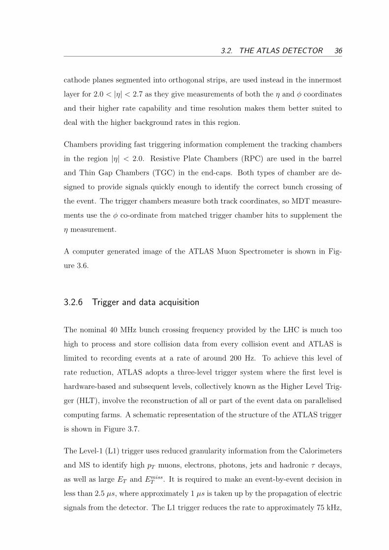
The trigger efficiencies for muons and electrons at each stage of the trigger chain,

are presented for the 8 TeV data in Figure 3.8.

The Data Acquisition (DAQ) system controls the movement of data through the trig-


ger system and to permanent storage and also manages the configuration and mon-

itoring of the ATLAS detector during data-taking. The average size of a recorded

event is approximately 1.3 Mb.

3.3 Data Sample

The results presented in this thesis are based on the data collected by ATLAS during

LHC Run I, between 2010 and 2012, where the LHC operated first at√s = 7 TeV

and later at√s = 8 TeV. Only events recorded in periods where all detector compo-

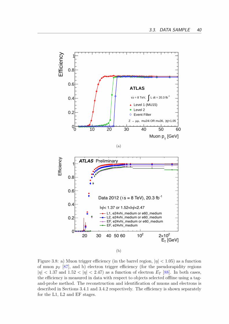
nents were operating normally are considered. The cumulative collected luminosity

during LHC Run I is illustrated in Figure 3.9.

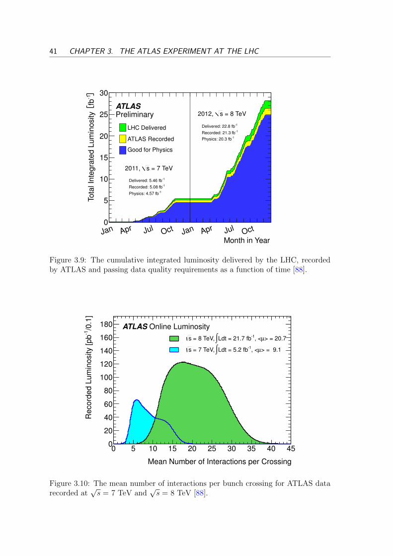
The average number of interactions per bunching crossing for the√s = 7 TeV and

√s = 8 TeV datasets is shown in Figure 3.10. As the LHC operated with a bunch

spacing of 50 ns, rather than the design bunch spacing of 25 ns, a high number of

protons per bunch was required to maintain a high instantaneous luminosity, leading

to a higher average number of interactions per bunch crossing than the design value.

The√s = 7 TeV and

√s = 8 TeV data samples used are summarised in Table 3.1.

Table 3.1: Summary of the√s = 7 TeV and

√s = 8 TeV data samples. The

“Data quality efficiency” column indicates the fraction of the delivered integratedluminosity collected when all detector components were functioning normally, andcorresponds to the “Good for Physics” histogram in Figure 3.9.

Year√s Instantaneous peak Average Data Data taking Data quality

luminosity Pile-up (< µ >) efficiency efficiency2011 7 TeV 3.65 ×1033cm−2s−1 9.1 4.5 fb−1 ≈96.5% ≈89.9%2012 8 TeV 7.73 ×1033cm−2s−1 20.3 20.3 fb−1 ≈95.5% ≈95.3%

3.3. DATA SAMPLE 40

[GeV]T

Muon p

0 10 20 30 40 50 60

Effi

cien

cy

0

0.2

0.4

0.6

0.8

1

ATLAS

-1 L dt = 20.3 fb∫ = 8 TeV, s

|<1.05η, mu24i OR mu36, |µµ →Z

Level 1 (MU15)

Level 2Event Filter

(a)

[GeV]TE20 30 40 50 60 210 210×2

Effic

ienc

y

0

0.2

0.4

0.6

0.8

1

L1, e24vhi_medium or e60_mediumL2, e24vhi_medium or e60_mediumEF, e24vhi_medium or e60_mediumEF, e24vhi_medium

|<2.47d|< 1.37 or 1.52<|d|

-1 = 8 TeV), 20.3 fbsData 2012 (

ATLAS Preliminary

(b)

Figure 3.8: a) Muon trigger efficiency (in the barrel region, |η| < 1.05) as a functionof muon pT [87], and b) electron trigger efficiency (for the pseudorapidity regions|η| < 1.37 and 1.52 < |η| < 2.47) as a function of electron ET [88]. In both cases,the efficiency is measured in data with respect to objects selected offline using a tag-and-probe method. The reconstruction and identification of muons and electrons isdescribed in Sections 3.4.1 and 3.4.2 respectively. The efficiency is shown separatelyfor the L1, L2 and EF stages.


Month in YearJan Apr Jul

Oct Jan Apr JulOct

1fb

Tota

l In

teg

rate

d L

um

inosity

0

5

10

15

20

25

30

ATLAS

Preliminary

= 7 TeVs2011,

= 8 TeVs2012,

LHC Delivered

ATLAS Recorded

Good for Physics

1 fbDelivered: 5.461 fbRecorded: 5.08

1 fbPhysics: 4.57

1 fbDelivered: 22.81 fbRecorded: 21.3

1 fbPhysics: 20.3

Figure 3.9: The cumulative integrated luminosity delivered by the LHC, recordedby ATLAS and passing data quality requirements as a function of time [88].

Mean Number of Interactions per Crossing

0 5 10 15 20 25 30 35 40 45

/0.1

]1

Record

ed L

um

inosity [pb

0

20

40

60

80

100

120

140

160

180 Online LuminosityATLAS

> = 20.7µ, <1Ldt = 21.7 fb∫ = 8 TeV, s

> = 9.1µ, <1Ldt = 5.2 fb∫ = 7 TeV, s

Figure 3.10: The mean number of interactions per bunch crossing for ATLAS datarecorded at

√s = 7 TeV and

√s = 8 TeV [88].

3.3. DATA SAMPLE 42

3.3.1 Luminosity Measurement

A precise measurement of the luminosity is important for many ATLAS analyses,

in particular for cross section measurements.

Using several event and particle counting algorithms with the ID, calorimeters and

dedicated luminosity detectors, ATLAS monitors the luminosity delivered by the

LHC by measuring the observed average number of interactions per bunch crossing.

The delivered luminosity, L, may be written as:

L =µnbfrσinelastic

=µvisnbfrσvis

(3.5)

where nb is the number of bunches, fr is the LHC revolution frequency, µ is the

number of inelastic interactions per bunch crossing and σinelastic is the total inelastic

cross section [89]. The number of visible inelastic interactions (excluding diffractive

processes which do not register signals in the relevant detectors) and the visible

inelastic cross section may be written as µvis = εµ and σvis = εσinelastic respectively,

where ε is the efficiency of a given detector and algorithm.

Since the ATLAS monitoring measures µvis, the absolute luminosity scale is given

by σvis. In terms of the accelerator parameters, the luminosity can alternatively be

expressed as:

L =nbfrn1n2

2πΣxΣy

(3.6)

where n1,2 are the number of protons in each bunch, and Σx,y are the horizontal

and vertical convolved beam widths [89]. The calibration of σvis is performed using

dedicated beam-separation scans known as Van der Meer scans [90, 91]. Via these

scans, Σx and Σy are measured directly and combining these with measurements of

the bunch populations n1,2 gives an absolute luminosity measurement.


3.4 Physics object reconstruction and identification

3.4.1 Muons

In ATLAS muon momentum is measured separately in the ID and MS. Four sets of

reconstruction criteria are used depending on the information available from the var-

ious sub-detectors, resulting in four categories: combined muons (CB), stand-alone

muons (SA), segment-tagged muons (ST) and calorimeter-tagged muons (CaloTag) [92].

In most cases, muons are identified by matching full or partial tracks from the MS

with ID tracks. For detector regions where either the ID or MS lacks coverage,

alternative strategies are used.

- Combined muons are the primary muon type used in ATLAS analyses,

where muon candidates are identified by matching an MS track with an ID

track and the track parameters are obtained by combining the two measure-

ments. Combined muons have the highest purity of the ATLAS muon types.

- Segment-tagged muons are muons that have not traversed all MS stations,

either because they have low pT or because their trajectories pass through

regions which are not fully instrumented. ST muons are identified using ID

tracks which, when extrapolated to the MS, match with a reconstructed track

segment. In this case, the track parameters of the ID track are assigned to the

muon.

- Stand-alone muons are reconstructed using only information from the MS.

The MS track is extrapolated back to the interaction point, taking into account

effects from multiple scattering and energy loss in the traversed material when

determining compatibility with the primary vertex. SA muons are used in the

region 2.5 < |η| < 2.7, outside of the geometrical acceptance of the ID.

- Calorimeter-tagged muons are used in the region |η| < 0.1 where the MS

is only partially instrumented. Muons are reconstructed using ID tracks with

3.4. PHYSICS OBJECT RECONSTRUCTION AND IDENTIFICATION 44

pT > 15 GeV, where the track is associated with an energy deposit in the

calorimeter compatible with a muon. The track parameters of the ID track

are assigned to the muon.

The reconstruction of muons using information from the MS (CB, SA and ST)

is performed using two separate algorithms which implement differently both the

reconstruction of tracks in the MS and the combination of ID and MS information.

The ‘Chain 1’ reconstruction algorithm combines the track parameters of the ID and

MS tracks using the corresponding covariance matrices and the ‘Chain 2’ algorithm

refits the muon track using the hits from both the ID and MS. The algorithms also

use different pattern recognition strategies for building tracks in the MS. The H →

ZZ(∗) → 4` analysis, described in detail in this thesis, uses muons reconstructed

with the ‘Chain 1’ algorithm.

The combination of muon reconstruction types results in a reconstruction efficiency

of around 99% for the majority of the geometrical acceptance of the detector. The

use of ST muons allows the recovery of efficiency in MS regions only partially in-

strumented, in particular 1.1 < |η| < 1.3, and the use of CaloTag muons similarly

allows for a significant increase in efficiency in the uninstrumented region |η| < 0.1.

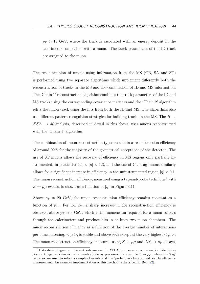
The muon reconstruction efficiency, measured using a tag-and-probe technique1 with

Z → µµ events, is shown as a function of |η| in Figure 3.11

Above pT ≈ 20 GeV, the muon reconstruction efficiency remains constant as a

function of pT . For low pT , a sharp increase in the reconstruction efficiency is

observed above pT ≈ 3 GeV, which is the momentum required for a muon to pass

through the calorimeters and produce hits in at least two muon chambers. The

muon reconstruction efficiency as a function of the average number of interactions

per bunch crossing, < µ >, is stable and above 99% except at the very highest< µ >.

The muon reconstruction efficiency, measured using Z → µµ and J/ψ → µµ decays,

1Data driven tag-and-probe methods are used in ATLAS to measure reconstruction, identifica-tion or trigger efficiencies using two-body decay processes, for example Z → µµ, where the ‘tag’particles are used to select a sample of events and the ‘probe’ paricles are used for the efficiencymeasurement. An example implementation of this method is described in Ref. [92].


-2.5 -2 -1.5 -1 -0.5 0 0.5 1 1.5 2 2.5

Effi

cien

cy

0.6

0.65

0.7

0.75

0.8

0.85

0.9

0.95

1

CB, MC CB, Data

CB+ST, MC CB+ST, Data

CaloTag, MC CaloTag, Data

ATLAS

Chain 1 Muons = 8 TeVs-1L = 20.3 fb > 10 GeV

Tp

η

-2.5 -2 -1.5 -1 -0.5 0 0.5 1 1.5 2 2.5

Dat

a / M

C

0.981

1.02

Figure 3.11: Muon reconstruction efficiency as a function of η, measured in Z →µµ events using muons with pT >10 GeV and reconstructed using the ‘Chain 1’algorithm and different muon reconstruction types. The error bars on the efficienciesrepresent the statistical uncertainties. The bottom panel shows the ratio betweenmeasured and predicted efficiencies. The error bars on the ratios show the totaluncertainties, combining the statistical and systematic components. Figure fromRef. [92].


is shown as a function of pT and < µ > in Figure 3.12.

20 40 60 80 100 120

Effi

cien

cy

0.9

0.92

0.94

0.96

0.98

1

Z MC MCψJ/

Z Data DataψJ/

ATLAS

Chain 1 CB + ST Muons = 8 TeVs

-1L = 20.3 fb| < 2.5η0.1 < |

[GeV]T

p

20 40 60 80 100 120

Dat

a / M

C

0.991

1.01

2 4 6 80

0.5

1

(a)

10 15 20 25 30 35 40 45 50

Effi

cien

cy

0.9

0.92

0.94

0.96

0.98

1

MC

Data

ATLASChain 1 CB + ST Muons

-1L = 20.3 fb

= 8 TeVs

> 10 GeVT

p| < 2.5η0.1 < |

⟩ µ ⟨

10 15 20 25 30 35 40 45 50

Dat

a / M

C

0.991

1.01

(b)

Figure 3.12: Reconstruction efficiency for CB+ST muons reconstructed with the‘Chain 1’ algorithm as a function of: a) the pT of the muon, for muons with 0.1< |η| < 2.5 using Z → µµ and J/ψ → µµ decays, and b) the average number ofcollisions per bunch crossing, < µ > for muons with 0.1 < |η| < 2.5 and pT > 10GeV. The panels at the bottom show the ratio between the measured and predictedefficiencies. The green bands show the statistical uncertainty only and the orangebands show the total uncertainty. Figure from Ref. [92].

Corrections derived from observed Z → µµ and J/ψ → µµ decays events are applied

to the simulation of the muon reconstruction to match the momentum scale and res-

olution measured in data. The use of J/ψ → µµ events in deriving the correction sig-

nificantly improves the precision in the low momentum range, which is particularly

important for the measurement of the Higgs boson mass in the H → ZZ(∗) → 4`

final state. Figure 3.13 shows a validation of this correction, where the peak position

and width of the J/ψ, Z and Υ resonances in data and simulation are fitted with

and without the correction applied. As Υ decays were not used in the derivation of

the correction, they provide an independent validation sample.

3.4.2 Electrons

The reconstruction of electrons in ATLAS combines information from the ID and the

LAr EM calorimeter, where background discrimination is provided by the shower

shape information available from the calorimeter, high-threshold TRT hits and the


of the leading muonη-2 -1 0 1 2

MC µµ

/ m

Dat

aµµ

m

0.995

0.996

0.997

0.998

0.999

1

1.001

1.002

1.003

1.004

1.005ATLAS

CB muons=8 TeVsData 2012,

-1 L dt = 20.3 fb∫

µµ →Z µµ → Υ

µµ → ψJ/

(a)

> [GeV]T

<p10 210

MC µµ

/ m

Dat

aµµ

m

0.995

0.996

0.997

0.998

0.999

1

1.001

1.002

1.003

1.004

1.005ATLAS

|<2.5ηCB muons |

=8 TeVsData 2012,

-1 L = 20.3 fb∫

µµ →Z µµ → Υ

µµ → ψJ/

(b)

Figure 3.13: Ratio of the reconstructed dimuon invariant mass for data to that insimulation for Z → µµ, Υ → µµ and J/ψ → µµ events: (a) as a function of the ηof the highest pT muon, and (b) as a function of the average transverse momentum< pT > of the two muons. The coloured bands show the systematic uncertainty onthe simulation corrections. Figure from Ref. [93].

compatibility of the tracking and calorimeter information. The details of the electron

reconstruction and identification are different for the√s = 7 TeV and

√s = 8 TeV

datasets [94] [95].

Electron candidates are reconstructed by matching a track in the ID with a cluster

of energy deposited in the EM calorimeter. The calorimeter cluster is required to

satisfy a number of criteria related to its longitudinal and transverse shower profiles.

Track candidates associated with the EM cluster are fitted using a Gaussian Sum

Filter (GSF) to take into account energy losses through bremsstrahlung [96]. For

the 8 TeV dataset, the ATLAS reconstruction was modified to account for larger

bremsstrahlung energy losses and to improve track-to-cluster matching, resulting

in an average increase in electron reconstruction efficiency of 5% for electrons with

ET > 15 GeV and 7% for ET < 15 GeV.

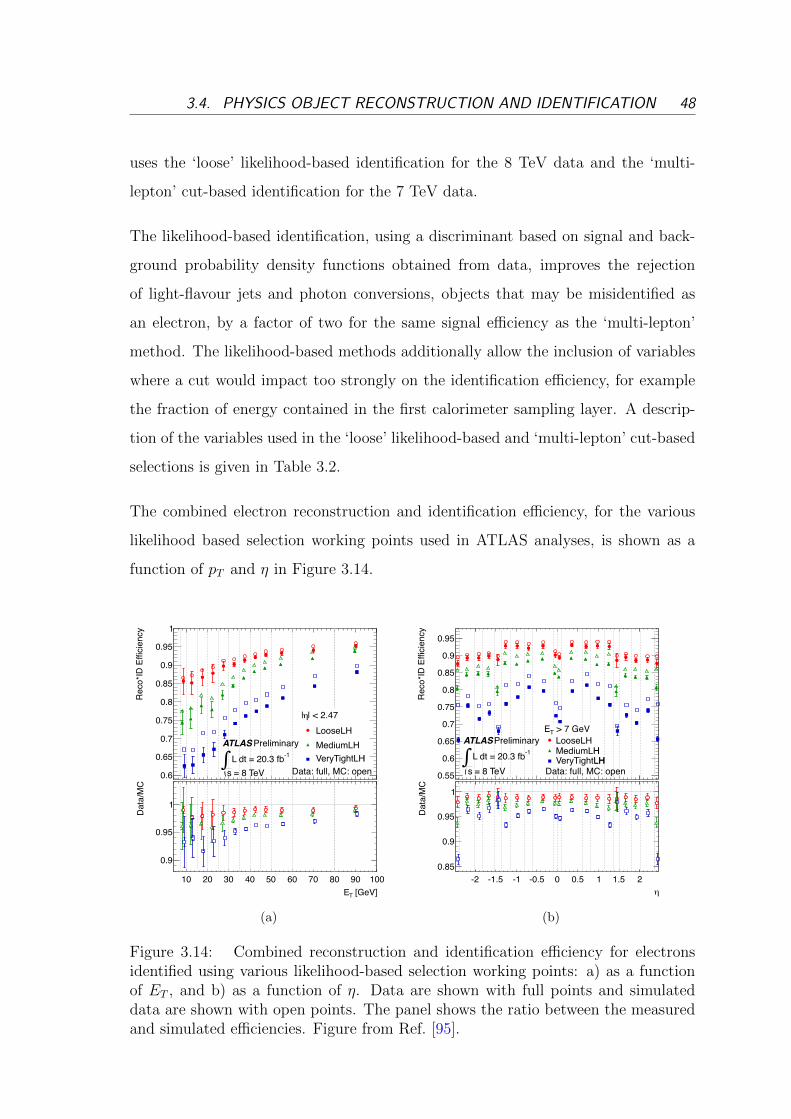
ATLAS analyses use a range of cut-based (i.e. a set of cuts on multiple input

variables) and likelihood-based selections to identify electrons, where typically the

most stringent selections are applied in final states which are subject to higher

backgrounds and, to maintain as large as possible an acceptance, looser cuts are

used in final states with lower backgrounds. The ATLAS H → ZZ(∗) → 4` analysis


uses the ‘loose’ likelihood-based identification for the 8 TeV data and the ‘multi-

lepton’ cut-based identification for the 7 TeV data.

The likelihood-based identification, using a discriminant based on signal and back-

ground probability density functions obtained from data, improves the rejection

of light-flavour jets and photon conversions, objects that may be misidentified as

an electron, by a factor of two for the same signal efficiency as the ‘multi-lepton’

method. The likelihood-based methods additionally allow the inclusion of variables

where a cut would impact too strongly on the identification efficiency, for example

the fraction of energy contained in the first calorimeter sampling layer. A descrip-

tion of the variables used in the ‘loose’ likelihood-based and ‘multi-lepton’ cut-based

selections is given in Table 3.2.

The combined electron reconstruction and identification efficiency, for the various

likelihood based selection working points used in ATLAS analyses, is shown as a

function of pT and η in Figure 3.14.

10 20 30 40 50 60 70 80 90 100

Rec

o*ID

Effi

cien

cy

0.6

0.65

0.7

0.75

0.8

0.85

0.9

0.95

1

-1 L dt = 20.3 fb∫ = 8 TeV s

ATLASPreliminary

| < 2.47η|LooseLHMediumLHVeryTightLH

Data: full, MC: open

| < 2.47η|LooseLHMediumLHVeryTightLH

[GeV]TE10 20 30 40 50 60 70 80 90 100

Dat

a/M

C

0.9

0.95

1

(a)

-2 -1.5 -1 -0.5 0 0.5 1 1.5 2

Rec

o*ID

Effi

cien

cy

0.55

0.6

0.65

0.7

0.75

0.8

0.85

0.9

0.95

-1 L dt = 20.3 fb∫ = 8 TeV s

ATLASPreliminary > 7 GeVTELooseLHMediumLHVeryTightLH

Data: full, MC: open

> 7 GeVTELooseLHMediumLHVeryTightLH

η-2 -1.5 -1 -0.5 0 0.5 1 1.5 2

Dat

a/M

C

0.85

0.9

0.95

1

(b)

Figure 3.14: Combined reconstruction and identification efficiency for electronsidentified using various likelihood-based selection working points: a) as a functionof ET , and b) as a function of η. Data are shown with full points and simulateddata are shown with open points. The panel shows the ratio between the measuredand simulated efficiencies. Figure from Ref. [95].

49 CHAPTER 3. THE ATLAS EXPERIMENT AT THE LHCT

able

3.2:

Defi

nit

ion

ofdis

crim

inat

ing

vari

able

suse

dfo

rel

ectr

onid

enti

fica

tion

usi

ng

the

mult

ilep

ton

cut-

bas

edcr

iter

iaan

dlo

ose

like

lihood

crit

eria

[95]

.T

heRφ

andf 1

vari

able

sar

enot

use

din

the

mult

ilep

ton

crit

eria

and

then

TR

Tva

riab

leis

not

use

din

the

loos

elike

lihood

crit

eria

.

Typ

eD

escr

ipti

onN

am

eH

adro

nic

leak

age

Rat

ioofE

Tin

the

firs

tla

yer

of

the

had

ron

icca

lori

met

ertoE

Tof

the

EM

clu

ster

RHad1

(use

dov

erth

era

nge|η|<

0.8

an

d|η|>

1.3

7)

Rat

ioofE

Tin

the

had

ronic

calo

rim

eter

toE

Tof

the

EM

clu

ster

RHad

(use

dov

erth

era

nge|η|>

0.8

an

d|η|<

1.3

7)

Th

ird

layer

ofR

atio

ofth

een

ergy

inth

eth

ird

layer

toth

eto

tal

ener

gy

f 3E

Mca

lori

met

er

Mid

dle

layer

ofL

ater

alsh

ower

wid

th,√ (Σ

Eiη

2 i)/

(ΣEi)−

((ΣEiηi)/(

ΣEi)

)2,

wh

ereEi

isth

eWη2

EM

calo

rim

eter

ener

gyan

dη i

isth

ep

seu

dora

pid

ity

of

celli

an

dth

esu

mis

calc

ula

ted

wit

hin

aw

ind

owof

3×

5ce

lls

Rat

ioof

the

ener

gyin

3×3

cell

sov

erth

een

ergy

in3×

7ce

lls

cente

red

at

the

Rφ

elec

tron

clu

ster

pos

itio

n(n

ot

use

dfo

rm

ult

ilep

ton

)R

atio

ofth

een

ergy

in3×

7ce

lls

over

the

ener

gy

in7×

7ce

lls

cente

red

at

the

Rη

elec

tron

clu

ster

pos

itio

n

Str

ipla

yer

ofS

how

erw

idth

,√ (Σ

Ei(i−i m

ax)2

)(ΣEi)

,w

her

ei

run

sov

erall

stri

ps

ina

win

dow

Wstot

EM

calo

rim

eter

of∆η×

∆φ≈

0.0

625×

0.2,

corr

esp

on

din

gty

pic

all

yto

20

stri

ps

inη,

an

di m

ax

isth

ein

dex

ofth

ehig

hes

t-en

ergy

stri

pR

atio

ofth

een

ergy

diff

eren

ceb

etw

een

the

larg

est

an

dse

con

dla

rges

ten

ergy

Era

tio

dep

osit

sin

the

clu

ster

over

the

sum

of

thes

een

ergie

sR

atio

ofth

een

ergy

inth

est

rip

layer

toth

eto

tal

ener

gy

(not

use

dfo

rm

ult

ilep

ton

)f 1

Tra

ckqu

alit

yN

um

ber

ofh

its

inth

eB

-lay

er(d

iscr

imin

ate

sagain

stp

hoto

nco

nve

rsio

ns)

nBlayer

Nu

mb

erof

hit

sin

the

pix

eld

etec

tor

nPixel

Nu

mb

erof

tota

lh

its

inth

ep

ixel

an

dS

CT

det

ecto

rsnSi

Mom

entu

mlo

stby

the

track

bet

wee

nth

ep

erig

eean

dth

ela

st∆p/p

mea

sure

men

tp

oint

div

ided

by

ori

gin

al

mom

entu

mT

RT

Tot

alnu

mb

erof

hit

sin

the

TR

T(n

ot

use

dfo

rlo

ose

like

lih

ood

)nTRT

Rat

ioof

the

nu

mb

erof

hig

h-t

hre

shold

hit

sto

the

tota

lnu

mb

erof

hit

sin

the

TR

TFHT

(rT

RT

)T

rack

–clu

ster

∆η

bet

wee

nth

ecl

ust

erp

osi

tion

inth

est

rip

layer

an

dth

eex

trap

olate

dtr

ack

∆η 1

mat

chin

g∆φ

bet

wee

nth

ecl

ust

erp

osi

tion

inth

em

idd

lela

yer

an

dth

eex

trap

ola

ted

track

∆φ2


The electron ET is calculated using the measured energy of the calorimeter cluster,

corrected for energy lost before the calorimeter or deposited in neighbouring cells,

and the direction of the ID track at the interaction point. The precise determination

of the scale and resolution of the electron energy is important for the measurement

of the Higgs boson mass in this channel and the calibration, described in Ref. [97],

exploits multivariate techniques and relies on a detailed knowledge of the detector

geometry and material distribution. The energy scale calibration is cross checked

as a function of ET in bins of |η| using J/ψ → ee and Z → ee events, as shown in

Figure 3.15.

[GeV]TE

10 20 30 40 50 60 70 80 90 100

Sca

le∆

-0.02

-0.015

-0.01

-0.005

0

0.005

0.01

0.015

0.02-e+ e→ ψJ/

-e+ e→Z

Calibration uncertainty

|<0.60ηElectrons, |

ATLAS -1=20.3 fbtdL∫=8 TeV, s

(a)

[GeV]TE

10 20 30 40 50 60 70 80 90 100

Sca

le∆

-0.02

-0.015

-0.01

-0.005

0

0.005

0.01

0.015

0.02-e+ e→ ψJ/

-e+ e→Z


|<1.37ηElectrons, 0.60<|


(b)

[GeV]TE

10 20 30 40 50 60 70 80 90 100

Sca

le∆

-0.02

-0.015

-0.01

-0.005

0

0.005

0.01

0.015

0.02-e+ e→ ψJ/

-e+ e→Z




(c)

[GeV]TE

10 20 30 40 50 60 70 80 90 100

Sca

le∆

-0.02

-0.015

-0.01

-0.005

0

0.005

0.01

0.015

0.02-e+ e→ ψJ/

-e+ e→Z




(d)

Figure 3.15: Energy scale factors, ∆ Scale, between the nominal electron energyscale and the measured energy scale, using the J/ψ → ee and Z → ee cross checkanalyses: (a) for |η| < 0.6, (b) for 0.6< |η| < 1.37, (c) for 1.37< |η| < 1.82, and(d) for 1.82< |η| < 2.37. The systematic uncertainty on the electron energy scale isshown as the shaded area. Figure from Ref. [93].

In the ATLAS H → ZZ(∗) → 4` analysis, for electron candidates with ET <

30 GeV whose cluster ET and track pT agree within uncertainties, a combined fit of


the cluster energy and track momentum is performed to calculate the electron ET ,

improving the four-lepton mass resolution, m4` by approximately 4% for final states

containing electrons. The improvement is significant for electrons falling in the so-

called ‘crack-region’, 1.37 < |η| < 1.52, where the barrel and end-cap calorimeters

overlap and the energy resolution is typically poor.

3.4.3 Photons

Photons are used in the H → ZZ(∗) → 4` analysis as part of the Final State

Radiation (FSR) correction described in section 4.2.1. Photons are reconstructed

in ATLAS by searching for clusters in the EM calorimeter, where clusters without

matching ID tracks are classified as unconverted photon candidates and clusters

matched to pairs of tracks consistent with γ → e+e− conversions are classified as

converted photon candidates [98]. In some cases, clusters are reconstructed with

both photon and electron hypotheses.

The reconstruction efficiency for photons is almost 100%, though as some are misiden-

tified as electrons, the identification efficiency for photons with 30 < ET < 100 GeV

is around 83-95% for unconverted photons, and 87-99% for converted photons [99].

The photon energy scale uncertainty is similar for converted and unconverted pho-

tons, and is 0.2-0.3% for |η| < 1.37 and |η| > 1.82, and 0.6% for the intermediate

region [97]. It does not depend strongly on ET .

3.4.4 Jets

In the H → ZZ(∗) → 4` analysis, jets are used to distinguish between Higgs boson

production mechanisms as described in chapter 5.1. Jets are reconstructed in AT-

LAS using topological clusters of calorimeter cells with the anti-kt algorithm [100],

using a distance parameter of R = 0.4 for the H → ZZ(∗) → 4` analysis. Jets are

calibrated to the hadronic scale using simulation, where a Jet Energy Scale (JES)


correction, estimated using a combination of in situ techniques, is applied to account

for differences between data and simulation [101].

The uncertainty on the calibration ranges from below 1% in the central region to

3.5% for low pT jets at high |η| for the√s = 8 TeV data, which is reduced sig-

nificantly compared to the√s = 7 TeV data. The uncertainty on the jet energy

resolution is around 1% for jets with above pT > 100 GeV and around 3% for jets

with pT ≈ 20 GeV.

Jets originating from additional interactions in the bunch crossing are removed by

requiring that at least 50% (75%) of the energy within ∆R = 0.4 around the jet

axis are compatible with the primary vertex for the 7 (8) TeV data.

CHAPTER 4

H → ZZ(∗) → 4` with the ATLAS detector

Both the ATLAS and CMS experiments have observed a previously unknown particle

in the search for the Higgs boson [12, 13], and subsequent studies indicate that the

properties of the observed particle are consistent with those predicted for the Higgs

boson by the SM [3, 102]. The H → ZZ(∗) → 4` final state, where ` = e, µ, is one

of the most sensitive Higgs boson decay channels and played a key part in these

results, in particular due to the high signal-to-background ratio (S/B) and good

mass resolution.

This chapter describes the analysis of the H → ZZ(∗) → 4` final state using the

full dataset collected by ATLAS during LHC Run I, including the measurement

of the Higgs boson mass [93]. Chapter 5 is dedicated to a detailed discussion of

the categorisation of events by production mechanism and the subsequent measure-

ment of the signal strengths for different production modes in this channel [4]. The

corresponding results obtained by the CMS collaboration may be found in Ref [103].

53

4.1. EVENT SELECTION 54

4.1 Event selection

To obtain a sample of H → ZZ(∗) → 4` events, single-lepton and dilepton trigger

algorithms are used, where the trigger requirements include pT (ET ) thresholds

for muons (electrons). The pT and ET thresholds for the range of triggers used,

presented in Table 4.1, are higher for the 8 TeV data to account for the increased

number of interactions per bunch crossing. The trigger efficiency, with respect to the

offline analysis, is almost 100% for events with a four-lepton candidate containing

only electrons, and is greater than 97% for events with a four-lepton candidate

containing muons.

Table 4.1: Required pT and ET thresholds for the triggers used to select events inthe 7 TeV and 8 TeV datasets.

Trigger pT/ET threshold(s) (GeV)

7 TeVSingle muon 18

Single electron 20Di-muon 10-10

Di-electron 12-12Muon-electron 6-10

8 TeVSingle muon 24

Single electron 24Di-muon 13-13

Di-muon (asymm.) 8-18Di-electron 12-12

Muon-electron 8-12

Only events with at least one reconstructed vertex that has three associated tracks

with pT > 400 MeV are considered, and the primary vertex for a given event is de-

fined as the vertex whose associated tracks correspond to the greatest pT sum. Higgs

boson candidates are reconstructed by selecting two same-flavour, opposite-charge

lepton pairs, where the reconstruction and identification of muon and electron can-

didates is described in Sections 3.4.1 and 3.4.2 respectively. Events are categorised

as 4µ, 2e2µ, 2µ2e or 4e depending on the flavour of the of the lepton pairs and the

distinction between the 2e2µ and 2µ2e channels is discussed below.

55 CHAPTER 4. H → ZZ(∗) → 4` WITH THE ATLAS DETECTOR

To maximise the acceptance, all four types of muons introduced in Section 3.4.1 are

used, where each lepton quadruplet is allowed to have at most one SA or CaloTag

muon. CB, ST and SA muons are required to have pT > 6 GeV and CaloTag muons

are required to have pT > 15 GeV. Stand-alone muons are only considered in the

pseudorapidity region |η| > 2.5, outside the ID acceptance, and are required to have

hits in all three layers of the MS. CaloTag muons are restricted to |η| < 0.1 and, in

order to reject misidentified electrons, CaloTag muons which have the same ID track

as an electron are rejected. Electrons are required to have ET > 7 GeV. To require

that all selected leptons are associated with the primary vertex, lepton tracks are

required to a have longitudinal impact parameter (along the direction of the beam

axis), |∆z0|, of less than 10 mm with respect to the primary vertex. To reduce the

background from cosmic rays, an additional cut on the transverse impact parameter,

|∆d0| < 1 mm, is required for muons.

In each quadruplet the pT thresholds for the three highest pT leptons, chosen to

optimise the median expected significance1 calculated using simulated signal events

with mH = 125 GeV, are 20, 15 and 10 GeV. The four leptons are required to be

well separated, with ∆R > 0.10 required for same flavour leptons and ∆R > 0.20

required for different flavour leptons. For 4µ and 4e events, events containing an

opposite-charge, same-flavor dilepton pair with m`` < 5 GeV are removed to reject

J/ψ → `` decays. The lepton pair with mass, m12, closest to the Z boson mass,

mZ , is labelled the leading dilepton, while the second lepton pair, with mass m34, is

labelled the sub-leading dilepton.

In each event a mass window requirement, again chosen to maximise the median

expected significance, is applied to the invariant mass of each of the lepton pairs.

The invariant mass of the leading dilepton is required to be between 50 GeV and

106 GeV, and the invariant mass of the sub-leading dilepton is required to lie in

the range mmin < m34 < 106 GeV, where mmin = 12 GeV for m4` < 140 GeV, rises

1The median expected significance under the hypothesis of s signal events and b backgroundevents is given by [104]:

med[Z0] =√

2((s+ b)ln(1 + s/b)− s

4.1. EVENT SELECTION 56

linearly to mmin = 50 GeV at m4` = 190 GeV and stays at mmin = 50 GeV for

m4` > 190 GeV. In the case that more than one quadruplet satisfies the kinematic

selection requirements, the one with m12 value closest to mZ is retained. If more

than four leptons are identified and multiple quadruplets have the same m12 value,

the one with the highest m34 is selected. For events where the Higgs boson candidate

contains both muon and electron pairs, the event is placed in the 2e2µ category if

the leading dilepton is a di-electron pair and is placed in the 2µ2e category if the

leading dilepton is a di-muon pair. If more than one channel has a quadruplet

passing the selection, the channel with the highest expected signal rate, in the order

4µ ⇒ 2e2µ ⇒ 2µ2e ⇒ 4e from highest to lowest, is kept. Less than one event per

mille is expected to contain two quadruplets.

Track- and calorimeter-based isolation and impact parameter requirements are ap-

plied to the leptons to reduce the number of events from reducible background

processes containing fake or non-prompt leptons entering the signal region, where

selected leptons may result from misidentified jets or in-flight pion or kaon decays.

The normalised track isolation discriminant is defined as the sum of the transverse

momenta of tracks, ΣpT, inside a cone of ∆R < 0.2 around the lepton, excluding the

lepton track, divided by the lepton pT. Each lepton is required to have a normalised

track isolation discriminant of less than 0.15. Only tracks with at least four hits in

the pixel and silicon strip detectors (“silicon hits”) and pT > 1 GeV are considered

for muon candidates, and only tracks with at least nine silicon hits, including one

hit in the innermost pixel layer, and pT > 0.4 GeV are considered for electron

candidates.

The normalised calorimetric isolation discriminant [4] for muons is defined as the

sum of the energy collected in calorimeter cells, ΣET , inside an isolation cone of

0.20 around the muon, after subtracting the local muon ionisation energy, divided

by the muon pT. For electrons, the normalized calorimetric isolation is computed

as the sum of the topological cluster transverse energies inside a cone of 0.2 around

the electron cluster divided by the electron pT, where the cells corresponding to


the core of the electron cluster are excluded from the sum. Muons are required

to have a normalised calorimetric isolation less than 0.30, while for electrons the

corresponding value is 0.20. For both the track- and calorimeter-based isolation

any contributions arising from other leptons of the quadruplet are subtracted. For

the track isolation the contribution from any other lepton in the quadruplet within

∆R < 0.2 is subtracted. For the calorimetric isolation the contribution of any

electron in the quadruplet within ∆R < 0.18 is subtracted.

The transverse impact parameter significance, d0/σd0 , defined as the impact param-

eter in the transverse plane divided by its uncertainty, is required to be lower than

3.5 for muons and lower than 6.5 for electrons. A looser cut is used for electrons as

the electron impact parameter distribution is broader as a result of bremsstrahlung.

The combined reconstruction, identification and selection efficiency for the 8 TeV

dataset, calculated using simulated events with mH = 125 GeV, is 39% for the 4µ

final state, 27% for the 2e2µ/2µ2e final states and 20% for the 4e final state. For

the 7 TeV dataset the efficiency is reduced to 25% for the 2e2µ/2µ2e final states

and 17% for the 4e final state, as some improvements in the electron reconstruction

and identification procedure for the 8 TeV data are not applied to the 7 TeV data.

4.2 Higgs boson reconstruction

4.2.1 Final state radiation recovery

The H → ZZ(∗) → 4` process may also include radiative photon production. Where

it is identified, the Final State Radiation (FSR) photon is incorporated into the

four lepton invariant mass calculation. Applying such a correction improves the

four-lepton mass resolution and allows the recovery of events whose reconstructed

four-lepton mass lies outside the signal region due to the FSR, avoiding applying a

correction for this loss based on simulation.

4.2. HIGGS BOSON RECONSTRUCTION 58

The FSR process in Z boson decays is well modelled by simulation and ATLAS has

developed a method to include both collinear (where the ∆R between the muon

and cluster satisfies ∆Rcluster,µ < 0.15) and non-collinear (∆Rcluster,µ/e > 0.15) FSR

photons in the reconstruction of Z bosons. A method to include collinear photons

is applied to muons, and exploits the longitudinal segmentation of the ATLAS EM

calorimeter to reconstruct photons collinear to muons [105]. For electrons, collinear

FSR photons are included in the electromagnetic shower associated with the elec-

tron in the calorimeter so no special treatment is necessary. The non-collinear FSR

correction is performed both for final states with muons and final states with elec-

trons.

The ATLAS H → ZZ(∗) → 4` analysis searches for FSR photons corresponding to

leptons selected as part of the Higgs boson candidate. Since the probability for more

than one FSR photon with significant energy in a single event is negligible, at most

one FSR photon is allowed per event. FSR corrections are only considered for the

leading dilepton pair.

The collinear correction is only applied if 66 < mµµ < 89 GeV and mµµγ < 100 GeV.

Photon candidates are required to have ET > 1.5 GeV and f0 < 0.2 for ∆R < 0.08,

and ET > 3.5 GeV and f0 < 0.1 for 0.08 < ∆R < 0.15, where f0 is the fraction of the

calorimeter cluster energy deposited in the first sampling layer. The f0 requirement

discriminates against cases where the calorimeter activity is induced by the muon

itself, and the ET requirement is applied to reduce the background due to π0 decays.

If a collinear correction is not applied, a non-collinear correction may be applied if

m`` < 81 GeV and m``γ < 100 GeV. Photon candidates are required to be isolated

and have ET > 10 GeV. The upper bound on m`` is introduced to prevent applying

the correction for Initial State Radiation (ISR). If more than one FSR candidate

satisfying these requirements is found, then the photon with the highest ET is se-

lected.

Figure 4.1 shows the invariant mass distribution for Z → µµ events where a collinear


photon or a non-collinear photon is identified, both before and after applying the

correction. The observed and simulated data agree well and the distributions after

the correction are centred near mZ .

70 75 80 85 90 95 100

Events

/ 0

.5 G

eV

5

10

15

20

25

310×ATLAS

1Ldt = 20.3 fb∫ = 8 TeV: s

Collinear FSR

No FSR correction, data

No FSR correction, simulation

FSR correction, data

FSR correction, simulation

[GeV])γ(µµm70 75 80 85 90 95 100

Data

/MC

0.5

1

1.5

(a)

70 75 80 85 90 95 100

Events

/ 0

.5 G

eV

500

1000

1500

2000

2500ATLAS

1Ldt = 20.3 fb∫ = 8 TeV: s

Noncollinear FSR

No FSR correction, data

No FSR correction, simulation

FSR correction, data

FSR correction, simulation

[GeV])γ(µµm

70 75 80 85 90 95 100

Data

/MC

0.5

1

1.5

(b)

Figure 4.1: The invariant mass distribution for Z → µµ events where: a) a collinearFSR photon is identified, and b) a non-collinear photon is identified. In both casesthe observed data are shown before (triangles) and after (circles) the correction.Simulated data are also shown, where in both cases the red histogram shows thesimulated data before the correction and the blue histogram shows the simulateddata after the correction. Figure from Ref. [4].

The collinear FSR correction is expected to be applied to approximately 4% of events

passing the H → ZZ(∗) → 4` event selection, with an efficiency of 70% and a purity

of 85%. The non-collinear FSR correction is expected to be applied to around 1%

of events, with an efficiency of 60% and a purity greater than 95%.

4.2.2 Z-Mass Constraint

Exploiting the fact that in H → ZZ(∗) → 4` decays, the leading lepton pair is

typically produced by the on-shell decay of a Z boson, the four-lepton mass resolu-

tion can be improved by applying a Z-mass-constrained kinematic fit to the leading

dilepton pair. The kinematic fit uses a relativistic Breigt-Wigner distribution to

4.3. DISCRIMINATION AGAINST SM DIBOSON PRODUCTION 60

model the Z boson line shape and a Gaussian distribution to model the momentum

response function for each lepton, where the width of the Gaussian is fixed to the

expected lepton momentum resolution. Though the actual lepton response functions

do not precisely correspond to Gaussian distributions, more complicated momentum

response functions were found to give a similar performance. Additionally, though

the Z boson line shape is not exactly a Breit-Wigner distribution, replacing the

Breit-Wigner distribution in the kinematic fit with the Z boson line shape taken

directly from simulation has a negligible effect on the results. More details on the

procedure can be found in Ref. [106]. The effect of the Z-mass-constrained fit on

simulated H → ZZ(∗) → 4µ events, using the preliminary analysis documented

in Ref. [107], is shown before and after applying the collinear FSR correction in

Figure 4.2.

The improvement in the four-lepton mass resolution as a result of the Z-mass con-

straint is studied by fitting a Gaussian to the peak of the simulated four-lepton

invariant mass distribution for mH = 125 GeV in each final state, before and after

the constrained fit. The Z-mass constraint improves the four-lepton mass resolution

by 18% in the 4µ channel, 23% in the 2e2µ channel, 11% in the 2µ2e channel and

14% in the 4e channel. The simulated distributions after the correction are shown

in Figure 4.3 with the fitted Gaussians overlaid.

4.3 Discrimination against SM diboson production

A Boosted Decision Tree (BDT) is used to build a discriminant between the signal

and the ZZ∗ background events and the BDT reponse is used as a second discrim-

inant in the maximum likelihood fit. The variables used in the BDT are a Matrix

Element- (ME) based kinematic discriminant and the transverse momentum, p4`T ,

and pseudorapidity, η4`, of the four-lepton system. The BDT is trained using sim-

ulated H → ZZ(∗) → 4` events, generated for mH = 125 GeV, against qq → ZZ(∗)

events, where all events are required to pass the full analysis selection and fall in


[GeV]4lm90 95 100105110 115120125130135140

Eve

nts/

2 G

eV

0

20

40

60

80

100

120

140

160

180

200

220

240

γEvents w/ recovered FSR No Correction

ConstraintZMγFSR

ConstraintZ

+ MγFSR

Preliminary ATLASSimulation

Figure 4.2: Simulated four-muon invariant mass distribution for mH = 125 GeV, forevents where a collinear FSR photon has been identified. The mass distribution isshown for uncorrected events (blue histogram) and events where the collinear FSRcorrection is applied (purple dashed histogram). In both cases, the effect of applyingthe Z-mass constrained fit is shown, by a black histogram for the case with no FSRcorrection and a red histogram for the case with the correction. All distributionsare normalised to the same area [107].

4.3. DISCRIMINATION AGAINST SM DIBOSON PRODUCTION 62

[GeV]µ4m

80 100 120 140

/ 0.

5 G

eVµ4

1/N

dN

/dm

0

0.02

0.04

0.06

0.08

0.1

0.12

= 125 GeVHmGaussian fit

SimulationATLAS

µ4→ZZ*→H = 8 TeVs

0.01 GeV±m = 124.92 0.01 GeV± = 1.60 σ

: 17%σ 2±Fraction outside

With Z mass constraint

(a)

[GeV]µ2e2m

80 100 120 140

/ 0.

5 G

eVµ

2e2

1/N

dN

/dm

0

0.02

0.04

0.06

0.08

0.1 = 125 GeVHm

Gaussian fit

SimulationATLAS

µ2e2→ZZ*→H = 8 TeVs

0.01 GeV±m = 124.87 0.01 GeV± = 1.61 σ



(b)

[GeV]2eµ2m

80 100 120 140

/ 0.

5 G

eV2eµ2

1/N

dN

/dm

0

0.01

0.02

0.03

0.04

0.05

0.06

0.07

0.08

0.09


SimulationATLAS

2eµ2→ZZ*→H = 8 TeVs

0.01 GeV±m = 124.66 0.02 GeV± = 2.01 σ



(c)

[GeV]4em

80 100 120 140

/ 0.

5 G

eV4e

1/N

dN

/dm

0

0.01

0.02

0.03

0.04

0.05

0.06

0.07

0.08


SimulationATLAS

4e→ZZ*→H = 8 TeVs

0.02 GeV±m = 124.51 0.02 GeV± = 2.18 σ



(d)

Figure 4.3: Simulated H → ZZ(∗) → 4` four-lepton invariant mass distributionsincluding the Z-mass constrained fit for mH = 125 GeV in: a) the 4µ channel, b)the 2e2µ channel, c) the 2µ2e channel, and d) the 4e channel. A Gaussian fit to thesimulated events is overlaid in each channel, where the fit is performed in a symmet-ric range for the 4µ channel, and in an asymmetric range for the other channels toaccommodate effects in the tail of the distribution due to bremsstrahlung. Figurefrom Ref. [4].


the the mass window 115 < m4` < 130 GeV. The training is performed separately

for the different final states. The signal and background distributions used to train

the BDT, as well as the BDT response, are shown in Figure 4.4.

The ME kinematic discriminant, DZZ∗ [4], is designed to exploit the differences

between the signal and ZZ(∗) background kinematics. It is defined as the logarithm

of the ratio of the matrix element under the signal hypothesis to the matrix element

under the background hypothesis:

DZZ∗ = ln

(|Msig|2

|MZZ∗|2

)(4.1)

where Msig is the ME for the ggF-produced H → ZZ(∗) → 4` process and MZZ∗

is the ME for the qq → ZZ(∗) background process. Both the signal and background

MEs are computed at LO using MadGraph [108], assuming the SM spin-CP hy-

pothesis JP = 0+ and mH = m4` on an event-by-event basis for the signal ME. As

shown in Figure 4.5, the BDT including p4`T and η4` in addition to DZZ∗ provides

more discrimination, particularly at higher signal efficiencies, than DZZ∗ alone.

4.4 Background estimation

The primary background process contributing to the H → ZZ(∗) → 4` analysis

signal region, described in Section 4.1, is SM ZZ(∗) production, which is also char-

acterised by the presence of isolated leptons. This background is estimated using

simulated events, which are normalised to the SM cross section. In the fiducial

region selected by this analysis the estimate, both in terms of shape and normali-

sation, shows good agreement between the observed and simulated data in the high

mass region (& 2mZ), where only ZZ(∗) production is expected to make a significant

contribution. Discrimination between the signal and this background is provided by

the BDT introduced in Section 4.3. The small expected background contribution

from WZ events is also estimated using simulation.

4.4. BACKGROUND ESTIMATION 64

outputZZ*D-6 -4 -2 0 2 4 6 8

out

put /

0.5

ZZ

*1/

N d

N/d

D

0

0.05

0.1

0.15

0.2

0.25ATLAS Simulation

l4→ZZ*→H

-1Ldt = 4.5 fb∫ = 7 TeV s

-1Ldt = 20.3 fb∫ = 8 TeV s

=125 GeV)H

ggF (m

ZZ*

(a)

[GeV]l4T

p0 50 100 150 200 250 300 350

/ 10

GeV

l4 T1/

N d

N/d

p

0

0.05

0.1

0.15

0.2

0.25

0.3

0.35

0.4ATLAS Simulation

l4→ZZ*→H

-1Ldt = 4.5 fb∫ = 7 TeV s

-1Ldt = 20.3 fb∫ = 8 TeV s

=125 GeV)H

ggF (m

ZZ*

(b)

l4η-8 -6 -4 -2 0 2 4 6 8

/ 0.

5l4 η

1/N

dN

/d

0

0.02

0.04

0.06

0.08

0.1

0.12

0.14 ATLAS Simulation

l4→ZZ*→H

-1Ldt = 4.5 fb∫ = 7 TeV s

-1Ldt = 20.3 fb∫ = 8 TeV s

=125 GeV)H

ggF (m

ZZ*

(c)

outputZZ*BDT-1 -0.6 -0.2 0.2 0.6 1

out

put /

0.0

5Z

Z*

1/N

dN

/dB

DT

0

0.02

0.04

0.06

0.08

0.1

0.12ATLAS Simulation

l4→ZZ*→H

-1Ldt = 4.5 fb∫ = 7 TeV s

-1Ldt = 20.3 fb∫ = 8 TeV s

=125 GeV)H

ggF (m

ZZ*

(d)

Figure 4.4: Signal (red histograms) and background (blue histograms) event distri-butions used in the training of the BDT: a) for DZZ∗ , b) for p4`

T , and c) for η4`. TheBDT response distributions are shown in d). All distributions are normalised to thesame area [4].


Signal efficiency0 0.2 0.4 0.6 0.8 1

Bac

kgro

und

reje

ctio

n

0

0.2

0.4

0.6

0.8

1

ATLAS Simulation

l4→ZZ*→H

= 8 TeVs

outputZZ*D

outputZZ*BDT

(a)

Figure 4.5: Background rejection fraction versus signal efficiency when using onlyDZZ∗ to discriminate between signal and background events (red), and when usingthe full BDT (black). Figure from Ref. [4].


Several background processes with misidentified or non-isolated leptons also con-

tribute to the final state, where the background composition depends on the sub-

leading dilepton flavour and is thus different for the ``µµ and `èe channels. The

main backgrounds of this type are ``+ jets and tt. Their rates are estimated using

data-driven techniques. Different methods, described in the following sections, are

used to estimate the rates of these backgrounds in the ``µµ and `èe final states.

4.4.1 Estimate of the ``µµ background

Apart from the dominant ZZ(∗) production, the main background process contribut-

ing to ``µµ final states is the production of a Z boson accompanied by jets, denoted

Z + jets. Where events enter into the signal region, the muons selected in the

sub-leading dilepton come predominantly from heavy quark meson semi-leptonic

(heavy-flavour) decays, with the process denoted Zbb. There is a smaller contri-

bution from muons produced in π/K in-flight decays and this process is denoted

Z + light jets. There is also a contribution to the background from t production. To

estimate the rates of these background processes, four orthogonal control regions, de-

scribed below, are defined in order to separate the different background components.

A simultaneous maximum likelihood fit to the observed data in each of the control

regions is performed, where the mass of the leading dilepton, m12, is used as the

discriminating variable. The Z + jets background is expected to have m12 peaking

at the mass of the Z boson, whereas tt events are expected to have a broader dis-

tribution. The selection requirements for each of the control regions include criteria

designed to reduce the contributions from the signal and ZZ(∗) processes.

The Inverted impact parameter significance control region (or ‘inverted-d0’

control region) is defined by applying the analysis selection described in Section 4.1,

with the exception that the isolation criteria are not applied to the leptons compris-

ing the sub-leading dilepton, and at least one of these leptons is required to fail the

impact parameter significance requirements. This control region enhances the Zbb

and tt contributions.


The Inverted isolation control region is defined by applying the analysis selec-

tion, with the exception that at least one of the leptons comprising the sub-leading

dilepton is required to fail either (or both) the track- or calorimeter-based isolation

requirements. To ensure orthogonality with the ‘inverted-d0’ control region, both

leptons in the sub-leading pair are required to pass the impact parameter signifi-

cance requirements. This control region enhances contributions from Z + light jets

and tt events and its inclusion in the simultaneous fit complements the ‘inverted-d0’

control region as it allows for the extraction of the Zbb and Z+light jets components

of the Z + jets background, which would be impossible to distinguish from a single

control region as their m12 distributions are expected to be similar.

The Same-sign sub-leading dilepton control region (or ‘SS’ control region) is

defined by applying the analysis selection, with the exception that neither the impact

parameter nor the isolation requirements are applied to leptons in the sub-leading

pair, and these leptons are required to have the same charge. The ‘SS’ control

region is expected to have significant contributions from the Zbb, Z + light jets and

tt processes.

The eµ leading dilepton control region is defined by applying the analysis selec-

tion, with the exception that the leading dilepton is made up of an opposite-charge,

opposite-flavour lepton pair and neither the impact parameter nor the isolation re-

quirements are applied to leptons in the sub-leading pair. Leptons in the sub-leading

pair are required to have the same flavour, and may have the same or opposite charge.

An additional requirement on the dilepton invariant mass is applied to remove the

contribution of events with a Z boson candidate decaying to a pair of electrons or

muons. This control region is dominated by tt events.

For each control region, the number of events expected from each of the background

processes, as well as the corresponding relative composition, is shown in Table 4.2.

To express the fit results from different control regions in a common way, a reference

control region is defined where the full analysis selection, except for the impact


Table 4.2: The expected contribution, estimated using simulated events, for eachof the background processes in each control region used in the simultaneous fit, interms of the absolute number of events (first three rows) and their relative fraction(bottom three rows).

Background inv-d0 CR inv-iso CR SS CR eµ CRAbsolute number of expected events

Zbb 70.5± 0.6 19.5± 0.3 47.0± 0.7 0.4± 1.9Z + light jets 20± 3 29± 3 26± 3 0.0± 1.3tt 124.6± 1.3 25.2± 0.6 80.6± 1.1 159.6± 1.6

Relative fraction of expected eventsZbb 0.328± 0.005 0.265± 0.012 0.306± 0.007 0.003± 0.012Z + light jets 0.092± 0.013 0.393± 0.026 0.169± 0.016 0.000± 0.008tt 0.580± 0.009 0.342± 0.016 0.525± 0.011 0.997± 0.010

parameter and isolation criteria for the leptons in the sub-leading pair, is applied.

Fit results are expressed in terms of the number of events for each process in this

control region, where the ratios between the number of events in each of the fitted

control regions and the reference control region are treated as Gaussian-constrained

nuisance parameters, with the nominal values and statistical uncertainties taken

from simulation. This control region is expected to contain contributions from each

of the background processes, but also includes all signal events entering the signal

region so is not included directly in the fit. The ratios between the number of events

in each of the fitted control regions and the reference control region, calculated using

simulated events, are shown in Table 4.3 together with their statistical uncertainties.

Table 4.3: Ratios between the number of events in the control regions used inthe fit to the reference region described in the text, calculated using simulation.The uncertainties are due to the number of events in the simulated samples. Theratios for the inverted d0, finv−d0, inverted isolation, finv−iso, SS, fSS, and eµ leadingdilepton, feµ+µµ, control regions are shown.

Background finv−d0 finv−iso fSS feµ+µµZbb 0.751± 0.010 0.209± 0.005 0.653± 0.012 0.0005± 0.0003

Z + light jets 0.44± 0.09 0.52± 0.09 0.59± 0.10 0.000± 0.003tt 0.828± 0.012 0.167± 0.004 0.539± 0.009 1.201± 0.023

The Zbb and Z + light jets m12 distributions are modelled using the convolution of

a relativistic Breit-Wigner distribution and a Crystal Ball function, and the tt m12


distribution is modelled using a second-order Chebyshev polynomial. The variable

parameters of these two functions are required to be the same in each control region.

The nominal parameter values are determined by a fit to simulated events, and in

the fit to data are treated as Gaussian-constrained nuisance parameters, where the

Gaussian widths correspond to the statistical uncertainties on the parameters from

the fit to simulated data. The small expected contributions from the WZ and SM

ZZ(∗) processes that enter the control regions are also modelled in the fit by the

convolution of a relativistic Breit-Wigner distribution and a Crystal Ball function,

where the yields are fixed to those predicted by simulation.

Several cross-checks are performed to validate the fit:

- The yields resulting from the fit to the simulated data are checked against the

number of events expected for each background component. The results are

found to be compatible within uncertainties.

- Two alternative fits are performed to the observed data. For the first all pa-

rameters are fixed to the predicted values from simulation, and for the second

the parameters are unconstrained in the fit. In both cases, the results are

compatible with the nominal results within uncertainties.

The m12 distribution, as well as the result of the maximum likelihood fit, are shown

for the observed data in each of the control regions used in the fit in Figure 4.6. The

corresponding estimated number of events in the reference control region is shown in

Table 4.4. The number of events for each background component as determined by

the simultaneous fit is shown, as well as the number of events determined by inde-

pendent maximum likelihood fits in each control region. The results are compatible

given the uncertainties.

The estimated number of events for each process in the reference control region is

extrapolated to the signal region using a ‘transfer factor’, the per-event probability

for the particular background type to fulfil the additional selection criteria (the

isolation and d0 requirements), calculated using simulated events. The calculated


[GeV]12m

50 60 70 80 90 100

Eve

nts

/ 4

Ge

V

0

10

20

30

40

50

60

70

80

DataTotal background

tt

bZ+bZ+lightflavor jets

WZ, ZZ*

ATLAS1Ldt = 4.5 fb∫ = 7 TeV s

1Ldt = 20.3 fb∫ = 8 TeV s

Inverted isolation control regionµµ+ll

(a)

[GeV]12m

50 60 70 80 90 100

Eve

nts

/ 4

Ge

V

0

20

40

60

80

100

120


tt


WZ, ZZ*


1Ldt = 20.3 fb∫ = 8 TeV s

control region0

Inverted dµµ+ll

(b)

[GeV]12m

50 60 70 80 90 100

Eve

nts

/ 4

Ge

V

0

20

40

60

80

100

120


tt


WZ, ZZ*


1Ldt = 20.3 fb∫ = 8 TeV s

Same sign control regionµµ+ll

(c)

[GeV]12m

50 60 70 80 90 100

Eve

nts

/ 4

Ge

V

0

10

20

30

40

50

60

70

80

Data

Total background

tt


WZ, ZZ*


1Ldt = 20.3 fb∫ = 8 TeV s

Control regionµµ+µe

(d)

Figure 4.6: Observed m12 distributions for the 7 TeV and 8 TeV data, shown as filledpoints, and the results of the maximum likelihood fit for the four control regions: (a)‘inverted-d0’, (b) ‘inverted-isolation’, (c) ‘SS’, and (d) eµ leading dilepton. The fitresults show the total background (black line) as well as the individual components:Zbb (blue line) and Z+light jets (green line), tt (dashed red line), and combined WZand ZZ(∗) (dashed grey line), where the WZ and ZZ(∗) contributions are estimatedfrom simulation. Figure from ref. [4].

efficiencies are checked with data using Z → `` + µ candidate events, where the

impact parameter and isolation requirements are applied to the Z boson candidate

and events with a fourth lepton or with a dilepton with m`` < 5 GeV are rejected.

Based on the difference between data and simulation, a 1.6% uncertainty is added


Table 4.4: Number of estimated events for different background components in thereference `` + µµ control region for the 7 TeV and 8 TeV data. The results areshown for the simultaneous maximum likelihood fit and for independent maximumlikelihood fits in each control region. The statistical uncertainties on the fitted yieldsare also shown [4].

Reducible background yields for 4µ and 2e2µ in reference control region

Control region Zbb Z + light jets Total Z + jets tt

Inverted impact parameter 206± 18 208± 23Inverted isolation 210± 21 201± 24eµ+ µµ – 201± 12Same-sign dilepton 198± 20 196± 22

Combined fit 159± 20 49± 10 208± 22 210± 12

to the transfer factor.

The transfer factors are shown in Table 4.5. The quoted uncertainties include the

statistical uncertainty due to the size of the simulated sample, as well as the sys-

tematic uncertainty based on the agreement between data and simulation. The

uncertainties on the transfer factors are significantly larger than the statistical un-

certainties from the simultaneous fit, so these uncertainties dominate the uncertainty

on the background estimates in the signal region.

Table 4.5: The transfer factors for each background type, calculated using per-event efficiencies for simulated events to pass the analysis selection isolation andimpact parameter requirements. The uncertainties are dominated by the statisticaluncertainty on the number of simulated events satisfying the full analysis selectionrequirements for each process.

Reducible Background Transfer Factor (%)Zbb 3.10± 0.19

Z + light jets 3.0± 1.8tt 0.55± 0.09

The estimated number of events in the signal regions in the 4µ and 2e2µ final

states, as well as the associated uncertainties, are shown for each background type

in Table 4.6. The decomposition of the Z + jets background into the Zbb and the

Z + light jets contributions is also is shown.


Table 4.6: Estimates for the number of background events (excluding the SM ZZ(∗)

background) in the 4µ and 2e2µ signal regions for the√s = 7 TeV and

√s = 8

TeV data. The Z + jets and tt background estimates come from the simultaneousfit described in the text and the WZ contribution comes from simulation. TheZ + jets background estimate is also shown separately for the Zbb and Z + light jetsprocesses [4].

Background 4µ 2e2µ√s = 7 TeV

Z + jets 0.42± 0.21(stat)± 0.08(syst) 0.29± 0.14(stat)± 0.05(syst)tt 0.081± 0.016(stat)± 0.021(syst) 0.056± 0.011(stat)± 0.015(syst)

WZ expectation 0.08± 0.05 0.19± 0.10

Z + jets decomposition

Zbb 0.36± 0.19(stat)± 0.07(syst) 0.25± 0.13(stat)± 0.05(syst)

Z + light-flavor jets 0.06± 0.08(stat)± 0.04(syst) 0.04± 0.06(stat)± 0.02(syst)√s = 8 TeV

Z + jets 3.11± 0.46(stat)± 0.43(syst) 2.58± 0.39(stat)± 0.43(syst)tt 0.51± 0.03(stat)± 0.09(syst) 0.48± 0.03(stat)± 0.08(syst)

WZ expectation 0.42± 0.07 0.44± 0.06

Z + jets decomposition

Zbb 2.30± 0.26(stat)± 0.14(syst) 2.01± 0.23(stat)± 0.13(syst)

Z + light-flavor jets 0.81± 0.38(stat)± 0.41(syst) 0.57± 0.31(stat)± 0.41(syst)

4.4.2 Estimate of the `èe background

For `èe final states, the background in the signal region typically arises from jets

which have been misidentified as electrons. Three different methods are used to

estimate these background contributions, exploiting two types of control region con-

taining electrons with relaxed identification requirements (X):

- 3` + X: the full analysis selection is applied, except for the requirements on

the lowest ET electron, where the electron identification criteria and isolation

and impact parameter significance requirements are relaxed.

- ``+XX: the full analysis selection is applied, except for the requirements on

the sub-leading dilepton, where the identification requirements for both of the


electrons are relaxed.

Several methods, described in this section, are used to estimate the background

in `èe final states. In each method, electron candidates originating from different

sources are assigned one of the following classifications:

f - light flavour jets misidentified as electrons.

γ - electrons from photon conversions.

q - electrons from semi-leptonic heavy-flavour meson decays.

The methods for determining the `èe background measure inclusively different back-

ground sources, and include contributions not only from Z + jets but also from tt,

WZ and ZZ(∗). The expected contribution from ZZ(∗), estimated using simulated

events, is subtracted from the final estimate.

The baseline method for the background estimate, chosen as the method with the

smallest expected total uncertainty, is known as the ‘3`+X’ method and is described

in Section 4.4.2.1. Two further methods provide cross-checks; the ‘Transfer Factors’

method, described in Section 4.4.2.2, and the ‘Reco-Truth Unfolding’ method, de-

scribed in Section 4.4.2.3.

4.4.2.1 The 3`+X method

The 3`+X method uses a control region where the full analysis selection is applied,

apart from the lowest ET electron, where relaxed requirements are applied. For the

lowest ET electron, a track with minimal silicon hit requirements (at least 7 silicon

hits, with hits in at least two of the pixel layers) matching a calorimeter cluster

is required, where no further electron identification criteria, nor impact parameter

significance or isolation requirements, are applied. To suppress the ZZ(∗) contri-

bution, the electron candidates forming the sub-leading pair are required to have


the same-sign. After this requirement, 5% of the remaining events are estimated to

come from ZZ(∗) and this contribution is subtracted from the final estimate. In the

case that more than one quadruplet per event is built, all the quadruplets with the

same m12 are considered.

As the 3` + X control region contains three leptons passing the full selection,

the background composition for this method is simpler than methods estimating

the background using an `` + XX control region. This allows the use of a two-

dimensional maximum likelihood fit, where the observables used are the number

of hits in the innermost layer of the pixel detector, nB−layerhits , and the ratio of the

number of high-threshold to low-threshold TRT hits, rTRT . The fit extracts the

yields for the f , γ and q background components. Separation between the com-

ponents is possible using the fact that for most converted photons, the conversion

happens after the first pixel layer, and electrons typically produce a higher number

of high-threshold TRT hits than jets.

The templates used to model each of the background components are taken from a

simulated sample of events in an ``+X control region, where only the minimal silicon

hit requirements, described above, are applied to X. A correction is applied to the

templates to account for the observed difference in the nB−layerhits and rTRT variables

between data and simulation. As the expected contribution of the q component in

the control region is low, its yield is Gaussian-constrained to the number of events

expected from simulation, where the Gaussian width is set to be 20% of the expected

yield.

The result of the fit is shown in Figure 4.7. The background contributions from

the f , γ and q sources are unfolded as a function of the electron pT using the sPlot

method [109], which returns event-by-event a so-called sWeight for each component,

corresponding to the probability for X to be of f , γ or q type. The sWeights for

each component, which sum to one for each event, are extrapolated from the control

region to the signal region with transfer factors that depend on the efficiency for an

electron of the component type in question to pass all selection requirements.


Blayer

hitsn

0 1 2 3

Eve

nts

1

10

210

310

Data

38±f = 1290

13± = 62 γ 5±q = 21

Total


1Ldt = 20.3 fb∫ = 8 TeV s

(a)

TRTr

0 0.1 0.2 0.3 0.4 0.5E

ve

nts

/ 0

.02

5

1

10

210

310

Data

38±f = 1290

13± = 62 γ 5±q = 21

Total

ATLAS

1Ldt = 4.5 fb∫ = 7 TeV s

1Ldt = 20.3 fb∫ = 8 TeV s

(b)

Figure 4.7: Results of the two-dimensional maximum-likelihood fit in the 3` + Xcontrol region to: a) nB−layerhits and, b) rTRT . The plots show the data (filled points),the total background (solid blue histogram) and its various components, namely f(green dashed histogram), γ (blue dashed histogram) and q (red dashed histogram).All distributions are shown for the sum of the 4e and 2µ2e channels, though the fitsare performed separately in each channel. Figure from Ref. [4].

The efficiencies for electron candidates corresponding to each type to pass all selec-

tion requirements is found using simulated Z+X events and corrected for differences

between data and simulation. The relevant sample is selected by requiring a recon-

structed Z boson candidate decaying to a same-flavour, opposite-charge lepton pair

with pT > 20 GeV, both leptons satisfying the requirements of the analysis event

selection. To reduce the number of events in the sample where X is a genuine elec-

tron, EmissT in the events is required to be below 50 GeV. Any additional leptons

are required to be well separated from the leptons associated with the Z boson can-

didate, satisfying ∆R > 0.2(0.1) for different-(same-) flavour leptons. The electron

candidate X is required to satisfy the silicon hit requirements applied throughout

this section. The efficiencies used for the extrapolation are obtained in 8 pT bins for

each of the different background sources.

For the f background type, the simulation efficiency is corrected by a scale factor as a

function of pT , which ranges from 1.6 to 2.5 in pT bins. The γ background type is well


modelled by the simulation, where the data and simulation agree within 10%. For the

q background component, the efficiency is well modelled by simulation. Systematic

uncertainties of 30%, 20% and 25% are applied to the f , γ and q components,

respectively, due to the data-simulation correction. The fit results in the 3` + X

control region, the extrapolation factors and the estimated number of events in the

signal region are shown, summed over the 4e and 2e2µ channels, for each background

type in Table 4.7. The total expected number of background events in the 4e and

2e2µ channels, after the subtraction of the expected ZZ(∗) contribution, is shown in

the Summary Table 4.8.

Table 4.7: Using the 3` + X method to estimate the `` + ee background, the fitresults for each component in the 3`+X control region, the transfer factors used forextrapolation and the signal region yields for the reducible `` + ee background areshown. The estimates for the 2µ2e and 4e channels are summed. The uncertaintiesare the combination of the statistical and systematic uncertainties [4].

Type Fit yield in control region Extrapolation factor Yield in signal region√s = 7 TeV data

f 391 ± 29 0.010 ± 0.001 3.9 ± 0.9γ 19 ± 9 0.10 ± 0.02 2.0 ± 1.0q 5.1 ± 1.0 0.10 ± 0.03 0.51 ± 0.15√

s = 8 TeV data

f 894 ± 44 0.0034 ± 0.0004 3.1 ± 1.0γ 48 ± 15 0.024 ± 0.004 1.1 ± 0.6q 18.3 ± 3.6 0.10 ± 0.02 1.8 ± 0.5

4.4.2.2 The transfer factors method

This cross-check method uses a `` + XX control region, where the full analysis

selection is applied to the leading dilepton and the sub-leading dilepton is formed

using electron candidates with relaxed identification requirements (“X”) that each

fail at least one of the isolation or impact parameter significance requirements. The

yield in this control region is extrapolated to the signal region using the efficiency

for electron candidates coming from each background source to pass the full analysis

selection.


Electron candidates are classified as ‘Electron (E)’ or ‘Fake (F )’ using reconstruction-

based discriminating variables and events are placed into categories depending on

this classification, where the composition of the different background sources is dif-

ferent in each category. The categorisation allows a more accurate determination of

the efficiencies for background electron candidates from each source to pass the full

selection requirements.

A Z + X control region is used to estimate the efficiency for X to pass the full

selection requirements, needed to extrapolate the measured yield in the control

region to the signal region. Two alternative approaches are taken for this estimation,

addressing in different ways the different compositions of the Z + X and `` + XX

control regions.

The total expected number of background events in the 4e and 2e2µ channels is

shown in the Summary Table 4.8.

4.4.2.3 The reco-truth unfolding method

This cross-check method uses an `` + XX control region, which is similar to the

control region used for the method described in Section 4.4.2.2, except that no re-

quirements are placed on the isolation and impact parameter significance for electron

candidates comprising the sub-leading dilepton2. In the simulated ``+XX sample,

each reconstruction category is further decomposed in terms of all possible paired

combinations of the various background sources, f , q, γ and e. The e classification

is introduced because of the contributions from the signal and ZZ(∗) background

processes, which are present in this control region as the isolation and impact pa-

rameter significance requirements are no longer inverted. The yield observed in the

`` + XX control region is extrapolated to the signal region in bins of pT and η,

where the transfer factor in each bin is calculated using the weighted sum of each

combination of background sources (16) in each reconstruction category (4). The

2The requirements are inverted for the previous method.


expected contribution from events classified as ee is dominated by the signal and

SM ZZ(∗) contributions and is removed, where an additional subtraction is made to

subtract the remaining ZZ(∗) events in other categories.

The total expected number of background events in the 4e and 2e2µ channels is

shown in Table 4.8.

Table 4.8: Estimated number of background events using each `èe backgroundestimation method in the 2e2µ and 4µ categories. Results are displayed for the√s = 7 TeV and

√s = 8 TeV data for the full mass range. The “†” symbol

indicates which method is used to estimate the background normalisation appliedin the analysis. The other estimates come from methods used as cross-checks. Thefirst uncertainty shown is statistical, the second is systematic [4].

Method√s = 7 TeV data

√s = 8 TeV data

2µ2e

3`+X† 2.9± 0.5± 0.5 2.9± 0.3± 0.6``+XX Transfer Factor 2.2± 0.3± 1.1 2.5± 0.1± 0.9``+XX Transfer Factor b-enriched 2.8± 0.5± 0.8 3.2± 0.2± 0.9``+XX Reco–truth 2.8± 0.4± 1.0 2.9± 0.3± 0.3

4e

3`+X† 3.3± 0.5± 0.5 2.9± 0.3± 0.5``+XX Transfer Factor 2.0± 0.3± 0.9 2.4± 0.1± 0.9``+XX Transfer Factor b-enriched 3.4± 0.9± 0.8 2.9± 0.2± 0.8``+XX Reco–truth 2.6± 0.4± 0.9 2.8± 0.3± 0.3

4.4.3 Background control plots

The agreement between the observed data and the sum of the background esti-

mates for the different background components is shown to be good in a control

region where the full analysis selection is applied, except for the isolation and im-

pact parameter significance requirements on the leptons comprising the subleading

dilepton. The invariant mass distributions for the leading dilepton, m12, and sub-

leading dilepton, m34 are shown in this control region for `` + µµ and `` + ee final

states in Figure 4.8. The Z + jets and tt components are normalised to the results


of the baseline data-driven estimates.

[GeV]12m60 80 100

Events

/ 2

GeV

0

20

40

60

80

100

120

140

160

180

200

Data

=125 GeV)H

Signal (m

ZZ*

Z+jets

tt

WZ

Systematic uncertainty

ATLAS

1 Ldt = 4.5 fb∫ = 7 TeV s

1 Ldt = 20.3 fb∫ = 8 TeV s

µµ+ll

(a)

[GeV]12m60 80 100

Events

/ 2

GeV

0

20

40

60

80

100

120

140

160

180

200

Data

=125 GeV)H

Signal (m

ZZ*

tZ+jets, t


ATLAS

1 Ldt = 4.5 fb∫ = 7 TeV s

1 Ldt = 20.3 fb∫ = 8 TeV s

+eell

(b)

[GeV]34m50 100

Events

/ 5

GeV

0

20

40

60

80

100

120

140

160 Data

=125 GeV)H

Signal (m

ZZ*

Z+jets

tt

WZ


ATLAS

1 Ldt = 4.5 fb∫ = 7 TeV s

1 Ldt = 20.3 fb∫ = 8 TeV s

µµ+ll

(c)

[GeV]34m50 100

Events

/ 5

GeV

0

20

40

60

80

100

120

140

160

Data

=125 GeV)H

Signal (m

ZZ*

tZ+jets, t


ATLAS

1 Ldt = 4.5 fb∫ = 7 TeV s

1 Ldt = 20.3 fb∫ = 8 TeV s

+eell

(d)

Figure 4.8: Leading and subleading dilepton invariant mass distribtuions in a controlregion where the full analysis selection is applied, except for the isolation and impactparameter significance requirements on the sub-leading dilepton. The sample isdivided according to the flavour of the sub-leading dilepton. (a) and (b) show them12 distribution, in (a) for ``+ µµ events, and in (b) for ``+ ee events. (c) and (d)show the m34 distribution, in (a) for `` + µµ events, and in (b) for `` + ee events.The simulation is normalised to the data-driven background estimates. The dataare shown as filled points and the different background sources as filled histograms.The total background systematic uncertainty is represented by the hatched areas.Figure from Ref. [4].

4.5. SIGNAL AND BACKGROUND MODELLING 80

4.5 Signal and background modelling

The ATLAS results in the H → ZZ(∗) → 4` final state, obtained using the inclusive

analysis discussed in this chapter, employ a two-dimensional, maximum likelihood

fit to the four-lepton invariant mass, m4`, and the output of the BDT discussed in

section 4.3, OBDTZZ∗ , in the mass range 110 < m4` < 140 GeV. This section describes

the procedures used to build the signal and background probability density functions

(PDFs) used in the fit.

4.5.1 Signal modelling

The signal PDF used in the two-dimensional fit takes the following form:

P(m4`, OBDTZZ∗ | mH) = P(m4` | OBDTZZ∗ , mH) P(OBDTZZ∗ | mH)

'

(4∑

n=1

Pn(m4` | mH)θn(OBDTZZ∗ )

)P(OBDTZZ∗ | mH)

(4.2)

where θn defines four bins in OBDTZZ∗ (-1 – -0.5, -0.5 – 0, 0 –0.5 and 0.5 – 1) and

Pn is the probability density in m4` for the signal in a given θn bin. Since the m4`

distribution doesn’t vary significantly as a function of OBDTZZ∗ in each of the bins,

the product of the one-dimensional probability densities of m4` and OBDTZZ∗ is used.

The m4` and OBDTZZ∗ probability densities are obtained using a Kernel Density

Estimation technique [110], which sums Gaussian kernels with variable width over

an input set of points, provided here by the simulated distributions. The resulting

probability densities are smoothed distributions which are statistically consistent

with the input distributions and don’t suffer from potential effects due to finite bin

size that would be present if template histograms were used to model the distribu-

tions. Also, since the probability densities are continuous, the m4` distributions can


be shifted horizontally by arbitrary m4` values, a feature which is exploited in the

implementation of the energy scale systematics discussed in Section 4.6.

The m4` probability densities are produced using samples generated at 15 different

mH values in the range 115 - 130 GeV (at 0.5 GeV intervals for 123 < mH < 126 GeV

and at 1 GeV intervals elsewhere) and are parameterised as functions of mH . This

is achieved using B-spline interpolation [111], where the m4` value at a given point

in the distribution, for a particular mH , is the weighted sum of the corresponding

m4` value from distributions associated with the series of mH control points. The

weights are determined for each control point from a cubic B-spline basis function.

The expected signal yields for different values of mH are obtained from simulation

at each of the control points used for the probability density modelling. The yields

at intermediate mass points are then obtained using asecond B-spline on the same

basis. Combining the signal shapes with the normalisations results in the normalised

signal shapes which are continuously parameterised in mH . Figure 4.9 shows the

two dimensional probability density used for the signal process.

4.5.2 Background modelling

The background is modelled using two-dimensional probability densities. The qq →

ZZ(∗) and gg → ZZ(∗) background template shapes are obtained separately by

performing Kernel Density Estimation, using simulated events as input, in two di-

mensions to obtain a smooth, two-dimensional m4` −OBDTZZ∗ distribution.

For the other background processes in the ``+ µµ final states, the two-dimensional

probability density distributions are also derived from simulation, where the sim-

ulation agrees well with the observed data in the control regions discussed in Sec-

tion 4.4.1. The uncertainty on the shape of the probability density is evaluated by

varying the track isolation and impact parameter significance selections applied. For

other backgrounds in ``+ ee final states, the number of simulated events is not suf-

ficient to produce a smooth background model, so the probability density is derived


[GeV]l4m

out

put

ZZ

* B

DT

0

0.05

0.1

0.15

0.2

0.25

0.3

0.35

0.4

-1

-0.5

0

0.5

1

110 115 120 125 130 135 140

= 1.51)µ = 125 GeV H

(mSignal

l 4→ ZZ* →H -1

Ldt = 4.5 fb∫ = 7 TeV s

-1Ldt = 20.3 fb∫ = 8 TeV s

ATLAS Simulation

Figure 4.9: Two dimensional probability density for the signal,P(m4`, OBDTZZ∗ | mH), normalised to the expected total number of events inthe sum of all final states for the 2011 and 2012 datasets. The expected totalnumber of events assumes mH = 125 GeV and µ= 1.51. Figure from Ref. [4].

from the 3`+X data control region, weighted by the transfer factors to reflect the

signal region kinematics. Here, the shape uncertainties are obtained by taking the

difference between the default probability density and the alternative probability

densities obtained by using the control regions used for cross-checks.

The background probability densities for ``+ µµ and ``+ ee final states are shown

projected onto m4` in Figure 4.10. Figure 4.11 shows the full two-dimensional prob-

ability densities for the ZZ(∗) and Z + jets backgrounds.


[GeV]l4m

0 100 200 300 400 500

Eve

nts

/ 0.5

GeV

0

0.001

0.002

0.003

0.004

0.005

0.006

0.007

0.008

0.009

0.01

-1Ldt = 4.5 fb∫ = 7 TeV s-1Ldt = 20.3 fb∫ = 8 TeV s

ATLAS

µµ+llNorm. unc. (stat. + sys.)

+eellNorm. unc. (stat. + sys.)

(a)

[GeV]l4m

110 115 120 125 130 135 140E

vent

s / 0

.5 G

eV

0.002

0.004

0.006

0.008

0.01

0.012

0.014

0.016

0.018

0.02

-1Ldt = 4.5 fb∫ = 7 TeV s-1Ldt = 20.3 fb∫ = 8 TeV s

ATLAS

µµ+llNorm. unc. (stat. + sys.)

+eellNorm. unc. (stat. + sys.)

(b)

Figure 4.10: One dimensional probability density, P(m4`), projected onto m4` forthe `` + µµ and `` + ee: a) for 0 < mH < 500 GeV, and (b) for the reduced massrange, 110< mH < 140 GeV, in which the maximum likelihood fit is performed [4].

[GeV]l4m

out

put

ZZ

* B

DT

0

0.02

0.04

0.06

0.08

0.1

-1

-0.5

0

0.5

1

110 115 120 125 130 135 140

Background ZZ*

l 4→ ZZ* →H -1

Ldt = 4.5 fb∫ = 7 TeV s

-1Ldt = 20.3 fb∫ = 8 TeV s

ATLAS Simulation

(a)

[GeV]l4m

out

put

ZZ

* B

DT

0

0.005

0.01

0.015

0.02

0.025

-1

-0.5

0

0.5

1

110 115 120 125 130 135 140

Z+jets

l 4→ ZZ* →H -1

Ldt = 4.5 fb∫ = 7 TeV s

-1Ldt = 20.3 fb∫ = 8 TeV s

ATLAS Simulation

(b)

Figure 4.11: Two dimensional probability density, P(m4`, OBDTZZ∗ ) for: a) theZZ(∗) background, and (b) the Z + jets background [4].


4.5.3 Likelihood function

The signal and background probability densities discussed above are used to con-

struct a likelihood function, L, that depends on mH and µ:

L(mH , µ,θ) =

year∏i

finalstate∏j

Poisson(Nij|µ · Sij(mH ,θ) +Bij(θ))

·Nij∏k=1

Fij((m4`, OBDTZZ∗ )k,mH , µ,θ)

(4.3)

which is the product of the Poisson probability of observing Nij events, given the

expectation for the signal Sij and background Bij, multiplied with the product of

the values of the probability density Fij, for (m4`, OBDTZZ∗ )k of all events in the

2011 and 2012 data sets and each of the four final states. Fij is the weighted sum

of the signal and background probability densities. θ represents the set of nuisance

parameters used to model the effect of the systematic uncertainties described in

Section 4.6.

Confidence intervals are based on the profile likelihood ratio technique [104]. The

profile likelihood ratio Λ(mH) used for the measurement of the Higgs boson mass is:

Λ(mH) =L(mH , ˆµ(mH),

ˆθ(mH))

L(mH , µ, θ)(4.4)

where the signal strength, µ, is a free parameter in the fit. The single circumflex

(e.g. θ(µ)) denotes the unconditional maximum likelihood estimate of a parameter

and the double circumflex (e.g.ˆθ(µ)) denotes the conditional maximum likelihood

estimate for given fixed values of µ.

For the measurement of the signal strength, mH is fixed to its best-fit value and the

profile likelihood ratio is:


Λ(µ) =L(µ,

ˆθ(µ))

L(µ, θ)(4.5)

4.6 Systematic Uncertainties

Systematic uncertainties are modelled using nuisance parameters in the profile like-

lihood ratio, as described in Section 4.5.

The dominant sources of systematic uncertainty on the measurement of the Higgs

boson mass in the four-lepton final state are the muon momentum scale (see Fig-

ure 3.13) and electron energy scale (see Figure 3.15). The corresponding uncertain-

ties are calculated by modifying the momentum (energy) of a muon (electron) by a

scale factor and observing the shift in the m4l distribution.

The measurement of the muon momentum scale is discussed in Section 3.4.1. In the

muon pT range 6-100 GeV, the systematic uncertainty on the scale is around 0.04%

for |η| < 2.0, and is up to 0.2% for |η| > 2.0. The uncertainty is modelled using

a single nuisance parameter, where deviations to the scale as measured in both the

ID and MS are considered. The uncertainties on the measured Higgs boson mass

due to the muon momentum scale uncertainties are estimated to be 0.04% for the

4µ final state and 0.02% for the 2µ2e and 2e2µ final states.

The determination of the electron energy scale is discussed in Section 3.4.2, and its

precision is better than 0.1% for the full pseudorapidity and ET coverage. A total

of 24 nuisance parameters are used to model the electron and photon energy scale

uncertainties, with the sources described in Ref [97]. An additional nuisance param-

eter is used to model the electron momentum scale uncertainty, which is relevant for

the combination of electron track and calorimeter information. The corresponding

uncertainties on the measured Higgs boson mass are 0.04% for the 4e and 2µ2e final

states and 0.03% for the 2e2µ final state.

For the final Higgs boson mass measurement in the four-lepton channel, final states

4.6. SYSTEMATIC UNCERTAINTIES 86

including muons have a relatively higher weight than final states containing electrons

due to their better mass resolution. Taking this into account, the electron energy

scale uncertainty gives rise to a 0.01% uncertainty on the Higgs boson mass, whereas

the muon momentum scale uncertainty gives rise to a 0.03% uncertainty. Other

sources of systematic uncertainty are negligible for this measurement.

For measurements of the Higgs boson signal rate, there are systematic uncertainties

relating to the uncertainty on the trigger, reconstruction and identification efficien-

cies for muons and electrons. These uncertainties are calculated using simulation by

comparing the nominal event yield with the modified yield after applying weights

to events or individual physics objects corresponding to the various sources of sys-

tematic uncertainty.

Due to the presence of multiple high-pT leptons in the final state, the trigger effi-

ciency for the H → ZZ(∗) → 4` final state is high. The uncertainties on the trigger

efficiency are estimated by calculating the number of events that pass the full se-

lection criteria with and without the trigger requirement in the simulation. The

uncertainties on the signal yield due to the electron trigger efficiency uncertainty

and the muon trigger efficiency uncertainty are each less than 0.7%.

The uncertainty on the reconstruction and identification efficiency of muons is dis-

cussed in Section 3.4.1 and is modelled using a single nuisance parameter. The

associated estimated uncertainties on the signal strength measurement are 1.9%,

0.8% and 1.1% in the 4µ, 2µ2e and 2e2µ final states, respectively.

Uncertainties on the electron reconstruction and identification efficiency, discussed

in Section 3.4.2, are modelled using seven nuisance parameters, taking into account

different ET ranges: 7 < ET < 10 GeV, 10 < ET < 15 GeV, 15 < ET < 20 GeV

and ET > 20 GeV. The method is designed to model the correlations between

the systematic uncertainties in the H → ZZ(∗) → 4` analysis and analyses in

other Higgs boson decay modes, for example H → WW (∗) → `ν`ν. The systematic

uncertainties on the Higgs boson signal strength measurement due to uncertainties in


the electron reconstruction and identification efficiencies, estimated using simulated

events with mH = 125 GeV, are 4.4%, 1.7% and 3.3% for 4e, 2e2µ and 2µ2e final

states, respectively.

Based on the data-simulation comparison in a tag-and-probe study of the efficiency

of the isolation and impact parameter significance requirements applied in the anal-

ysis selection, an additional uncertainty is applied in two ET bins for electrons with

ET < 15 GeV. For electrons with ET < 11 GeV, the uncertainty is 1.4% in the barrel

region and 2.5% in the end-cap region. For electrons with 11 GeV< ET < 15 GeV,

the uncertainty is 0.7% in the barrel region and 1.2% in the end-cap region. For

simulated signal events with mH = 125 GeV, the additional systematic uncertain-

ties induced on the measurement of the Higgs boson signal strength are 1.2%, 0.1%

and 1.1% for the 4e, 2e2µ and 2µ2e final states, respectively. The corresponding

uncertainties for muons are found to be negligible.

There are also systematic uncertainties associated with the uncertainty on theoret-

ical calculations, the luminosity measurement and the data-driven estimates of the

rates of background processes. These are discussed in Sections 2.2, 3.3 and 4.4

respectively.

A summary of the systematic uncertainties on the measurement of the Higgs boson

signal strength in this channel may be found in Table 4.9.

4.7 Results

The event selection described in Section 4.1 is applied to the full 7 TeV and 8 TeV

datasets. In total, 428 events are selected with m4` > 100 GeV, with 137 events

selected in the 4µ final state, 212 in total in the 2e2µ and 2µ2e channels and 79 in

the 4e category. In this mass range, 371 ± 14 events are expected from background

processes alone.

Figure 4.12 shows the m4` distribution for the selected events, summed over all

4.7. RESULTS 88

Table 4.9: Impact of different sources of systematic uncertainty on the measurementof the Higgs boson signal strength for each of the final states considered in theanalysis, as well as their combination. Where a particular source of uncertaintyis negligible for a given final state, this is indicated with “–”. The systematicuncertainties related to theoretical uncertainties apply equally to all final states [4].

Source of uncertainty 4µ 2e2µ 2µ2e 4e combined

Electron reconstruction/identification – 1.7% 3.3% 4.4% 1.6%efficienciesElectron isolation/impact parameter – 0.07% 1.1% 1.2% 0.5%selectionElectron trigger efficiency – 0.21% 0.05% 0.21% <0.2%``+ ee backgrounds – – 3.4% 3.4% 1.3%

Muon reconstruction/identification 1.9% 1.1% 0.8% – 1.5%efficienciesMuon trigger efficiency 0.6% 0.03% 0.6% – 0.2%``+ µµ backgrounds 1.6% 1.6% – – 1.2%

QCD scale uncertainty 6.5%PDF, αs uncertainty 6.0%H → ZZ∗ branching ratio uncertainty 4.0%


final states, as well as the expected distributions for the signal and background

processes. Distributions are shown for the full mass range considered by the analysis

and for a reduced mass range, 80 GeV < m4` < 170 GeV. An excess of events above

the background-only prediction is visible in the region around m4` = 125 GeV.

Elsewhere, the data are well described by the background prediction.

Figure 4.13 shows the m12 and m34 distributions for the selected events, summed

over all final states, falling in the mass range used in the maximum likelihood fit,

110 GeV < m4` < 140 GeV, and the two-dimensional m12 − m34 distribution for

events with 120 GeV < m4` < 130 GeV. In both cases, the expected distributions

for signal and background events are also shown. The data are described well by

the simulation.

The distribution of BDTZZ(∗) for selected events with 120 GeV < m4` < 130 GeV for

the sum of all final states is shown in Figure 4.14, along with the two-dimensional

m4` − BDTZZ(∗) distribution for selected events with 110 GeV < m4` < 140 GeV.

The expected distributions for signal and background events are again shown. The

data are again observed to be compatible with the simulation.

For all of the Figures discussed above, the expected signal distributions are scaled

by a factor of µ = 1.51, the best-fit value for the Higgs boson signal strength at

mH = 125 GeV, as measured by the categorised analysis described in Chapter 5.

The observed number of events for each final state for the 7 TeV and 8 TeV datasets

is shown in Table 4.10 for the mass range 120 GeV < m4` < 130 GeV. The expected

number of signal and background events in this mass range is also shown, along

with the corresponding signal-to-background ratio. The collinear FSR correction is

applied to 8 selected events and the non-collinear correction is applied to 2 events.

This is in good agreement with the expected numbers from simulation.

The significance of the observed excess around m4` = 125 GeV is quantified via

the local p0-value, the probability for an excess at least as large as that observed

to occur under the background-only hypothesis. The p0-value is calculated under

4.7. RESULTS 90

[GeV]l4m

80 90 100 110 120 130 140 150 160 170

Eve

nts

/ 2.5

GeV

0

5

10

15

20

25

30

35 Data

= 1.51)µ = 125 GeV H

Signal (m

Background ZZ*

tBackground Z+jets, t


l 4→ ZZ* →H -1

Ldt = 4.5 fb∫ = 7 TeV s

-1Ldt = 20.3 fb∫ = 8 TeV s

ATLAS

(a)

[GeV]l4m

100 200 300 400 500 600

Eve

nts

/ 10

GeV

0

10

20

30

40

50

60

70

80Data

= 1.51)µ = 125 GeV H

Signal (m

Background ZZ*



l 4→ ZZ* →H -1

Ldt = 4.5 fb∫ = 7 TeV s

-1Ldt = 20.3 fb∫ = 8 TeV s

ATLAS

(b)

Figure 4.12: Four-lepton invariant mass distributions for events passing the eventselection, summing the 4µ, 2e2µ, 2µ2e and 4e final states, in the 7 TeV and 8 TeVdata sets: a) in the mass range 80 GeV < m4` < 170 GeV, and b) in the full massrange. The data are shown as filled circles and the expected signal and backgrounddistributions are shown as filled histograms. The ZZ(∗) background (red histogram)is shown separately from the Z + jets and tt backgrounds (purple histogram). Thesignal distribution (blue histogram) is shown for mH = 125 GeV and is scaled by asignal strength µ = 1.51. Figure from Ref. [4].


[GeV] 12m

50 60 70 80 90 100 110

[GeV

]34

m

20

30

40

50

60

70

80

0

0.02

0.04

0.06

0.08

0.1

0.12

0.14

0.16

0.18

0.2

< 130 GeVl4120 < m

Data

= 1.51)µ = 125 GeV H

Signal (m

Background ZZ*, Z+jets

l 4→ ZZ* →H -1

Ldt = 4.5 fb∫ = 7 TeV s

-1Ldt = 20.3 fb∫ = 8 TeV s

ATLAS

(a)

[GeV]12m

50 55 60 65 70 75 80 85 90 95 100

Eve

nts

/ 2.5

GeV

0

5

10

15

20

25

30

< 140 GeVl4110 < m

Data

= 1.51)µ = 125 GeV H

Signal (m

Background ZZ*



l 4→ ZZ* →H -1

Ldt = 4.5 fb∫ = 7 TeV s

-1Ldt = 20.3 fb∫ = 8 TeV s

ATLAS

(b)

[GeV]34m

15 20 25 30 35 40 45 50 55 60

Eve

nts

/ 4 G

eV

0

5

10

15

20

25

< 140 GeVl4110 < m

Data

= 1.51)µ = 125 GeV H

Signal (m

Background ZZ*



l 4→ ZZ* →H -1

Ldt = 4.5 fb∫ = 7 TeV s

-1Ldt = 20.3 fb∫ = 8 TeV s

ATLAS

(c)

Figure 4.13: a) m12 −m34, b) m12, and c) m34, distributions for events passing theevent selection for all 4` final states in the 7 TeV and 8 TeV data sets. Eventsin the mass range 120 GeV < m4` < 130 GeV are shown in a) and events in themass range 110 GeV < m4` < 140 GeV are shown in b) and c). In a) the expecteddistributions for the signal (blue) and total background (red) are shown, where therelative density of events is indicated by the box size for the signal and the colourshading for the background. In b) and c) The data are shown as filled circles andthe expected signal and background distributions are shown as filled histograms.The ZZ(∗) background (red histogram) is shown separately from the Z + jets and ttbackgrounds (purple histogram). The signal distribution (blue histogram) is shownfor mH = 125 GeV and is scaled by a signal strength µ = 1.51. Figure from Ref. [4].

4.7. RESULTS 92

[GeV]l4m

out

put

ZZ

* B

DT

0

0.02

0.04

0.06

0.08

0.1

-1

-0.5

0

0.5

1

110 115 120 125 130 135 140

Data

= 1.51)µ = 125 GeV H

Signal (m


l 4→ ZZ* →H -1

Ldt = 4.5 fb∫ = 7 TeV s

-1Ldt = 20.3 fb∫ = 8 TeV s

ATLAS

(a)

outputZZ*BDT-1 -0.8-0.6-0.4-0.2 0 0.2 0.4 0.6 0.8 1

Eve

nts

/ 0.2

0

2

4

6

8

10

12

14

16

18

< 130 GeVl4120 < m

Data

= 1.51)µ = 125 GeV H

Signal (m

Background ZZ*



l 4→ ZZ* →H -1

Ldt = 4.5 fb∫ = 7 TeV s

-1Ldt = 20.3 fb∫ = 8 TeV s

ATLAS

(b)

Figure 4.14: a) m4` − BDTZZ(∗) , and b) BDTZZ(∗) distributions for events passingthe event selection for all 4` final states in the 7 TeV and 8 TeV data sets: in themass range 120 GeV < m4` < 130 GeV for a), and 110 GeV < m4` < 140 GeVfor b). In a) the expected distributions for the signal (blue) and total background(red) are shown, where the relative density of events is indicated by the box sizefor the signal and the colour shading for the background. In b) the data are shownas filled circles and the expected signal and background distributions are shown asfilled histograms. The ZZ(∗) background (red histogram) is shown separately fromthe Z + jets and tt backgrounds (purple histogram). The signal distribution (bluehistogram) is shown for mH = 125 GeV and is scaled by a signal strength µ = 1.51.Figure from Ref. [4].


Table 4.10: The number of events observed after the full event selection for 120 <m4` < 130 GeV for the 7 TeV and 8 TeV datasets. The number of expected signalevents under the mH = 125 GeV hypothesis, number of expected ZZ(∗) events,number of Z + jets and tt events and corresponding signal-to-background ratio arealso shown [4].

Final Signal Signal ZZ(∗) Z + jets, tt S/B Exp. Obs.state full mass range √

s = 7 TeV

4µ 1.00 ± 0.10 0.91 ± 0.09 0.46 ± 0.02 0.10 ± 0.04 1.7 1.47 ± 0.10 22e2µ 0.66 ± 0.06 0.58 ± 0.06 0.32 ± 0.02 0.09 ± 0.03 1.5 0.99 ± 0.07 22µ2e 0.50 ± 0.05 0.44 ± 0.04 0.21 ± 0.01 0.36 ± 0.08 0.8 1.01 ± 0.09 14e 0.46 ± 0.05 0.39 ± 0.04 0.19 ± 0.01 0.40 ± 0.09 0.7 0.98 ± 0.10 1

Total 2.62 ± 0.26 2.32 ± 0.23 1.17 ± 0.06 0.96 ± 0.18 1.1 4.45 ± 0.30 6√s = 8 TeV

4µ 5.80 ± 0.57 5.28 ± 0.52 2.36 ± 0.12 0.69 ± 0.13 1.7 8.33 ± 0.6 122e2µ 3.92 ± 0.39 3.45 ± 0.34 1.67 ± 0.08 0.60 ± 0.10 1.5 5.72 ± 0.37 72µ2e 3.06 ± 0.31 2.71 ± 0.28 1.17 ± 0.07 0.36 ± 0.08 1.8 4.23 ± 0.30 54e 2.79 ± 0.29 2.38 ± 0.25 1.03 ± 0.07 0.35 ± 0.07 1.7 3.77 ± 0.27 7

Total 15.6 ± 1.6 13.8 ± 1.4 6.24 ± 0.34 2.00 ± 0.28 1.7 22.1 ± 1.5 31√s = 7 TeV and

√s = 8 TeV

4µ 6.80 ± 0.67 6.20 ± 0.61 2.82 ± 0.14 0.79 ± 0.13 1.7 9.81 ± 0.64 142e2µ 4.58 ± 0.45 4.04 ± 0.40 1.99 ± 0.10 0.69 ± 0.11 1.5 6.72 ± 0.42 92µ2e 3.56 ± 0.36 3.15 ± 0.32 1.38 ± 0.08 0.72 ± 0.12 1.5 5.24 ± 0.35 64e 3.25 ± 0.34 2.77 ± 0.29 1.22 ± 0.08 0.76 ± 0.11 1.4 4.75 ± 0.32 8

Total 18.2 ± 1.8 16.2 ± 1.6 7.41 ± 0.40 2.95 ± 0.33 1.6 26.5 ± 1.7 37

the asymptotic approximation [104] using the profile likelihood ratio test statistic

described in Section 4.5. The maximum p0-value, corresponding to 8.2 standard

deviations, is found to be at mH = 124.51 GeV, where the expected significance for

a SM Higgs boson of this mass is 5.8 standard deviations. At the ATLAS best-fit

value for the Higgs boson mass, mH = 125.36 GeV (discussed in section 4.7.1), the

p0-value corresponds to 8.1 standard deviations, where the expected significance is

6.2 standard deviations. The p0-value is shown as a function of mH in Figure 4.15.

4.7. RESULTS 94

[GeV]Hm120 122 124 126 128 130

0Lo

cal p Obs 2012

Exp 2012Obs 2011Exp 2011Obs combinationExp combination

ATLAS

l 4→ ZZ*→H-1Ldt = 4.5 fb∫=7 TeV s

-1Ldt = 20.3 fb∫=8 TeV s

σ2

σ4

σ6

σ8-1510

-1210

-910

-610

-310

1

Figure 4.15: Observed (solid lines) and median expected (dashed lines) distribu-tions for the local p0-value as a function of mH for the 7 TeV (red) and 8 TeV(blue) datasets and their combination (black). The dashed lines show p0-valuescorresponding to integer numbers of standard deviations. Figure from Ref. [4].


4.7.1 Higgs boson mass and inclusive signal strength measurement

The Higgs boson mass is measured using the selected H → ZZ(∗) → 4` events using

the profile likelihood ratio test statistic described in Section 4.5. Using the baseline

two-dimensional fit method, the best-fit value is:

mH = 124.51± 0.52(stat)± 0.06(syst)GeV

where the systematic uncertainty is calculated by taking the quadrature subtrac-

tion of the full fit uncertainty, minus the fit uncertainty when fixing the nuisance

parameters corresponding to systematic uncertainties to their best fit values. Using

the cross-check methods described in Section 4.5, similar best-fit values are obtained

for the Higgs boson mass, with the best-fit value from the one-dimensional method

within 120 MeV of the baseline value and the best-fit value from the per-event-errors

method with 60 MeV.

At mH = 124.51 GeV, the best-fit inclusive signal strength is µ = 1.66+0.45−0.38. At

the best-fit value for the Higgs boson mass obtained using the combination of the

H → ZZ(∗) → 4` and H → γγ channels in ATLAS (discussed in Section 4.7.1), the

best-fit value is found to be µ = 1.50+0.35−0.31(stat)+0.19

−0.13(syst).

The profile likelihood is shown as a function of the Higgs boson mass in Figure 4.16,

and as a function of the Higgs boson signal strength (with the Higgs boson mass

fixed to the ATLAS combined best-fit value, mH = 125.36GeV) in Figure 4.17. In

both cases, the results are shown for the individual channels and their combination.

4.7.1.1 ATLAS combined measurement

To improve the precision on the Higgs boson mass measurement, ATLAS performs

a combined fit to the observed events selected in the H → ZZ(∗) → 4` and H → γγ

final states, where the latter analysis is described in Ref. [93]. The measured Higgs

4.7. RESULTS 96

[GeV]Hm

Λ2

ln

0

2

4

6

8

10

12

14

121 123 125 127 129

4e

µ4

µ2e2

2eµ2

Combined

σ1

σ2

ATLAS

l 4→ ZZ* →H 1

Ldt = 4.5 fb∫ = 7 TeV: s

1Ldt = 20.3 fb∫ = 8 TeV: s Dashed without systematicsDashed without systematics

Figure 4.16: Profile likelihood as a function of the Higgs boson mass, mH , forthe combination of the 7 TeV and 8 TeV datasets. The 4µ (blue), 2µ2e (yellow),2e2µ (red) and 4e (green) channels are shown, together with the combination ofall channels (black). For the combination, the result is shown with (solid line) andwithout (dashed line) systematic uncertainties included. Figure from Ref. [93].


µSignal strength 0 0.5 1 1.5 2 2.5 3 3.5 4

Λ-2

ln

0

2

4

6

8

10

12

14

16

18

204e

µ4µ2e2

2eµ2CombinedNo syst. unc.

σ1

σ2

ATLAS -1

Ldt = 4.5 fb∫ = 7 TeV s

-1Ldt = 20.3 fb∫ = 8 TeV s

=125.36 GeVH

, ml4→ZZ*→H

Figure 4.17: Profile likelihood as a function of the Higgs boson signal strength, µ,for the combination of the 7 TeV and 8 TeV datasets. The 4µ (blue), 2µ2e (yellow),2e2µ (red) and 4e (green) channels are shown, together with the combination ofall channels (black). For the combination, the result is shown with (solid line) andwithout (dashed line) systematic uncertainties included. The value of the Higgsboson mass is fixed to the ATLAS combined best-fit value, mH = 125.36 GeV.Figure from Ref. [4].

4.7. RESULTS 98

boson mass using the H → γγ final state alone is mH = 125.98 ± 0.42(stat) ±

0.28(syst)GeV.

The profile likelihood ratio test statistic used for the combined mass measurement,

Λ(mH), is:

Λ(mH) =L(mH , ˆµ4`(mH), ˆµγγ(mH),

ˆθ(mH))

L(mH , µ4`, µγγ, θ)(4.6)

where the signal strengths for the four-lepton, µ4`, and diphoton, µγγ, decay modes

are profiled separately. The best-fit value for the Higgs boson mass from the com-

bined fit is mH = 125.36 ± 0.37(stat) ± 0.18(syst)GeV. As a cross-check, the fit

is also performed using a common, fixed signal strength, µ = 1, and the result is

found to lie within 80 MeV of the baseline value. The profile likelihood is shown as a

function of mH in Figure 4.18 for the individual decay modes and their combination.

For the H → ZZ(∗) → 4` final state the uncertainty is dominated by the statistical

component, whereas for the H → γγ final state the systematic uncertainty, though

smaller than the statistical uncertainty, has a non-negligable impact.

The compatibility between the mass measurements in the two decay modes is studied

by reparameterising the profile likelihood ratio above in terms of the difference

between the measured mass in each mode, ∆mH , profiling mH in the fit. The

compatibility, derived from the value of the profile likelihood ratio at ∆mH = 0,

corresponds to a significance of 1.98 standard deviations.

4.7.1.2 Combined ATLAS and CMS measurement

Using the full LHC Run I dataset, the ATLAS and CMS collaborations have per-

formed a simultaneous fit to the observed data samples in the H → ZZ(∗) → 4` and

H → γγ final states by each experiment [112]. The results for the Higgs boson

mass measurements performed by the CMS collaboration in the H → ZZ(∗) → 4`

and H → γγ channels may be found in Refs. [103] and [113] respectively, while the


[GeV]Hm

123 123.5 124 124.5 125 125.5 126 126.5 127 127.5

Λ-2

ln

0

1

2

3

4

5

6

7

σ1

σ2

ATLAS-1Ldt = 4.5 fb∫ = 7 TeV s

-1Ldt = 20.3 fb∫ = 8 TeV s

l+4γγCombined γγ →H

l 4→ ZZ* →H without systematics

Figure 4.18: Profile likelihood as a function of the Higgs boson mass, mH , forthe combination of the 7 TeV and 8 TeV datasets. The result is shown using theH → ZZ(∗) → 4` decay mode alone (blue), the H → γγ decay mode alone (red)and the combination (black). In each case, the result is shown with (solid line) andwithout (dashed line) systematic uncertainties included. Figure from Ref. [93].

) [GeV]l4 m− γγ = (mHm∆

-1 -0.5 0 0.5 1 1.5 2 2.5 3 3.5 4

Λ-2

ln

0

2

4

6

8

10

12

σ1

σ2(0)Λ-2ln

σ3

ATLAS-1Ldt = 4.5 fb∫ = 7 TeV s

-1Ldt = 20.3 fb∫ = 8 TeV s

Figure 4.19: Profile likelihood as a function of the difference between the measuredHiggs boson masses in the H → ZZ(∗) → 4` and H → γγ channels, ∆mH , for thecombination of the 7 TeV and 8 TeV datasets [93].

4.7. RESULTS 100

CMS combined Higgs boson mass measurement may be found in Ref. [114].

The procedure is similar to the procedure used for the ATLAS combination, and

the best-fit value for the Higgs boson mass is found to be:

mH = 125.09± 0.21(stat)± 0.11(syst)GeV

A summary of the measured masses in each channel for each experiment is shown

in Figure 4.20, along with the combined measurements for each experiment and the

overall combined measurement. The individual measurements are consistent with

each other.

[GeV]Hm124 125 126 127 1280.001

5

Total

Stat.

Syst.

CMS and ATLAS

Run 1LHCl+4γγ CMS+ATLAS

l4→ZZ→H CMS

l4→ZZ→H ATLAS

γγ→H CMS

γγ→H ATLAS

Figure 4.20: Measured mass of the Higgs boson for the H → ZZ(∗) → 4` and H →γγ channels in the ATLAS and CMS experiments, the combined mass measurementfor each experiment and the overall combination. The systematic uncertainties(magenta bands), statistical uncertainties (yellow bands) and total uncertainties(error bars) are shown. The red line shows the combined best-fit mass, and the greyline shows the total uncertainty on this measurement. Figure from Ref. [112].


4.7.2 Fiducial and differential cross section measurements

ATLAS has also measured fiducial and differential cross sections for Higgs boson

production in the H → ZZ(∗) → 4` final state using the 8 TeV dataset [5]. The

differential cross section measurements are performed in bins of six variables: the

transverse momentum of the four-lepton systems, p4`T , the pseudo-rapidity of the

four-lepton system, y4`, the dilepton invariant mass of the sub-leading lepton pair,

m34, the decay angle of the leading dilepton with respect to the beam axis in the four-

lepton rest frame, the number of jets per event, Njets, and the transverse momentum

of the leading jet, pjT .

Figure 4.21 shows the observed and expected distributions in four of these variables

- p4`T , m34, Njets and pjT - for events with 118 GeV < m4` < 129 GeV. In each case,

the observed data agree well with the prediction.

In a fiducial region designed to be as close as possible to the analysis selection

presented in Section 4.1, described in Ref. [5], the cross section is found to be

σfidtot = 2.11+0.53−0.47(stat)± 0.08(syst) fb. This is consistent with the theoretical predic-

tion for mH = 125.4 GeV σfidtot = 1.30± 0.13 fb [27].

ATLAS has also measured fiducial and differential Higgs boson cross sections in the

diphoton final state [115], and these results have been combined [116].

4.7. RESULTS 102

[GeV] recoHT,

p

0 20 40 60 80 100 120 140 160 180 200

Eve

nts

/ 20

GeV

2

4

6

8

10

12

14

16

18

20data

= 125 GeV)HmSignal (Background ZZ*

tBackground Z+jets, tSystematic uncertainty

ATLASl 4→ ZZ* →H

-1 L dt = 20.3 fb∫ = 8 TeV s

< 129 GeVl4m118 <

(a)

[GeV] reco34m

15 20 25 30 35 40 45 50 55 60

Eve

nts

/ 8 G

eV

5

10

15

20

25data




-1 L dt = 20.3 fb∫ = 8 TeV s

< 129 GeVl4m118 <

(b)

recojetsn

0 1 2 3≥

Eve

nts

5

10

15

20

25

30

35data




-1 L dt = 20.3 fb∫ = 8 TeV s

< 129 GeVl4m118 <

(c)

[GeV] recoT,jet

p

0 20 40 60 80 100 120 140

Eve

nts

/ 20

GeV

2468

1012141618202224

data = 125 GeV)HmSignal (

Background ZZ*



-1 L dt = 20.3 fb∫ = 8 TeV s

< 129 GeVl4m118 <

(d)

Figure 4.21: a) p4`T , b) m34, c) Njets, and d) p4`

T , for selected events, summing the 4µ,2e2µ, 2µ2e and 4e final states, in the mass range 118 GeV < m4` < 129 GeV for the8 TeV data. The expected signal distributions for mH = 125 GeV are shown (bluefilled histograms), as are the expected ZZ(∗) (red filled histograms) and Z+jets andtt (purple filled histograms) background distribution. Figure from Ref. [5].

CHAPTER 5

Higgs boson production rates and couplings in the

H → ZZ(∗) → 4` channel

This chapter contains a detailed discussion of the ATLAS collaboration measurement

of the production rates and couplings of the Higgs boson in the H → ZZ(∗) → 4`

decay mode using the full LHC run I dataset [4]. The results supercede those from

the preliminary analysis described in Ref [107].

5.1 Event categorisation

To extract the rates for different Higgs boson production mechanisms, events pass-

ing the H → ZZ(∗) → 4` selection requirements detailed in 4.1 are categorised to

gain the sensitivity to discriminate between Higgs boson production modes. Se-

lected events are assigned to one of the following four categories - VBF-enriched,

VH-hadronic enriched, VH-leptonic enriched and ggF-enriched - where the first three

103

5.1. EVENT CATEGORISATION 104

categories apply requirements on top of the usual event selection based on the char-

acteristic signatures of the VBF and VH Higgs boson production modes.

This categorisation is summarised in the schematic diagram in Figure 5.1 and the

following sections discuss the VBF-enriched , VH-hadronic enriched and VH-leptonic

enriched categories in more detail. Candidates not assigned to any of these categories

are placed in the ggF-enriched category.


selectionl4

High mass two jets

VBFVBF enriched

Low mass two jets

jj)H→ jj)H, Z(→W(

Additional lepton

)Hll →)H, Z(νl →W(

VH enriched

ggF ggF enriched

Figure 5.1: Schematic representation of the event categorisation procedure for theH → ZZ(∗) → 4` measurement of Higgs boson production rates and couplings.Events passing the selection requirements described in Section 4.1 are assigned toone of four categories which are tested sequentially: VBF-enriched, VH-hadronicenriched, VH-leptonic enriched or ggF-enriched [4].

105 CHAPTER 5. HIGGS BOSON PRODUCTION RATES AND COUPLINGS INTHE H → ZZ(∗) → 4` CHANNEL

5.1.1 VBF enriched category selection criteria

The signature of the VBF Higgs boson production mechanism is the presence of two

high transverse momentum jets, well separated in pseudorapidity.

VBF-like events are selected by requiring that the Higgs boson candidate is accom-

panied by at least two jets with pT > 25 (30) GeV for |η| < 2.5 (2.5 < |η| < 4.5). If

more than two jets are identified per event, the two highest pT jets are selected as

the VBF-tagged jets. Selecting instead the two jets comprising the highest invariant

mass di-jet candidate in the event has negligible impact on the expected sensitivity.

The selection criteria for the VBF-enriched and VH-hadronic enriched categories are

required to be orthogonal, so only events where the di-jet mass of the VBF-tagged

jets is greater than 130 GeV are selected as VBF-enriched, with negligible impact

on the sensitivity of the category.

The selection efficiency of the VBF-enriched category is estimated to be 55% using

a simulated sample of events in the VBF production mode. A considerable fraction

of the events entering the category, estimated to be 54% from simulation, are pro-

duced via the ggF mechanism, so to discriminate between VBF and ggF events a

BDT classifier, labelled BDTVBF, is used. The response of this BDT is used as an

observable in the VBF-enriched category in a multi-observable maximum likelihood

fit, described in Section 5.4.

5.1.1.1 Boosted Decision Tree classifier for VBF enriched category

The BDT classifier designed to discriminate between events produced by the VBF

and ggF production mechanisms, BDTVBF, is trained using simulated VBF events

as signal and simulated ggF events as background. The classifier input variables

are:

- The invariant mass of the tagged di-jet system, mjj


- The pseudorapidity separation between the two tagged jets, |ηjj|

- The transverse momentum of each tagged jet, p1,2T

- The pseudorapidity of the highest pT jet, η1

where the variables are ranked in order of separation1, which gives an indication of

the relative discriminating power of each of the BDT input variables.

The distributions of the BDT input variables and the overall BDT response are

shown in Figure 5.2. As expected, the distributions indicate that Higgs boson events

produced via the VBF mechanism typically have a higher di-jet invariant mass and

larger pseudorapidity separation than events produced via the ggF mechanism. The

pT spectra of the leading and sub-leading tagged jets peak at higher pT values for

events produced via the VBF mechanism.

The BDT response is found to be similar for ggF produced signal events and for

the ZZ(∗) background. Combining the simulated ggF and ZZ(∗) events to form the

background sample for the training has a negligible impact on the results.

Additional variables have been tested as input variables to the BDT. These include

additional kinematic observables:

- The di-jet transverse momentum, pjjT

- The azimuthal separation between the di-jet system and the four-lepton sys-

tem, φ4`,jj

- The pseudo-rapidity of a third jet (when present), η3

- The angular distance between the four-lepton system and the closest jet ∆R4`,jj

1The separation provided by a variable, x, is calculated via the integral:

1

2

∫(xS(x)− xB(x))2

xS(x) + xB(x)

where xS(x) and xB(x) are the signal and background PDFs.


[GeV]jj

m

200 400 600 800 1000

/ 1

0 G

eV

jj1/N

dN

/dm

0

0.02

0.04

0.06

0.08

0.1 Simulation ATLAS

l 4→ ZZ* →H 1

Ldt = 4.5 fb∫ = 7 TeV s1

Ldt = 20.3 fb∫ = 8 TeV s

categoryVBF enriched

=125 GeVH

m

ggF

VBF

(a)

|jj

η∆|

0 1 2 3 4 5 6 7 8

| / 0.2

jjη∆1/N

dN

/d|

0

0.02

0.04

0.06

0.08


l 4→ ZZ* →H

1Ldt = 4.5 fb∫ = 7 TeV s

1Ldt = 20.3 fb∫ = 8 TeV s


=125 GeVH

m

ggF

VBF

(b)

[GeV]T

Leading Jet p

50 100 150 200 250 300 350 400

/ 1

0 G

eV

T1/N

dN

/dp

0

0.02

0.04

0.06

0.08

0.1

0.12

0.14

0.16

0.18

0.2

Simulation ATLAS

l 4→ ZZ* →H

1Ldt = 4.5 fb∫ = 7 TeV s

1Ldt = 20.3 fb∫ = 8 TeV s


=125 GeVH

m

ggF

VBF

(c)

[GeV]T

Subleading Jet p

50 100 150 200

/ 4

GeV

T1/N

dN

/dp

0

0.05

0.1

0.15

0.2

0.25

Simulation ATLAS

l 4→ ZZ* →H

1Ldt = 4.5 fb∫ = 7 TeV s

1Ldt = 20.3 fb∫ = 8 TeV s


=125 GeVH

m

ggF

VBF

(d)

ηLeading Jet

4 3 2 1 0 1 2 3 4

/ 0

.2η

1/N

dN

/d

0

0.01

0.02

0.03

0.04

0.05

0.06

Simulation ATLAS

l 4→ ZZ* →H

1Ldt = 4.5 fb∫ = 7 TeV s

1Ldt = 20.3 fb∫ = 8 TeV s


=125 GeVH

m

ggF

VBF

(e)

outputVBF

BDT

1 0.6 0.2 0.2 0.6 1

/ 0

.05

VB

F1/N

dN

/dB

DT

0

0.02

0.04

0.06

0.08

0.1

0.12Simulation ATLAS

l 4→ ZZ* →H

1Ldt = 4.5 fb∫ = 7 TeV s

1Ldt = 20.3 fb∫ = 8 TeV s


=125 GeVH

m

ggF

VBF

ZZ*

(f)

Figure 5.2: Distribution of input variables for the VBF (green histograms) andggF (blue histograms) event samples used in the training of the BDT: (a) dijetinvariant mass, (b) dijet η separation, (c) leading jet pT, (d) sub-leading jet pT and(e) leading jet η. (f) BDTVBF response for VBF and ggF events, as well as for theZZ∗ background (red). All histograms in a given figure are normalised to the samearea [4].


and variables designed to differentiate between gluon-induced and quark-induced

jets:

- The number of tracks in a jet

- The jet width, W , which is defined as:

W =Σi∆R

ipiTΣiP i

T

where i are the jet constiuents [117].

For the addition of any of the variables above, at most a small improvement in

the discriminating power between VBF and ggF events is achieved. Since for these

variables differences are seen between the observed and simulated data, the addition

of any of these variables to the BDT would necessitate adding additional systematic

uncertainties, negating any improvements in the discriminating power.

The dependence of the output of the BDT discriminant on the Higgs boson mass

is negligible, and so the training used four simulated samples with mH=123, 124,

126 and 127 GeV for each of the ggF and VBF processes. These samples are split

evenly into training and testing samples. Training is performed separately for the 7

TeV and 8 TeV datasets to take the difference in kinematics into account.

5.1.2 VH-hadronic enriched category selection criteria

For Higgs boson production in association with a hadronically decaying electroweak

boson, a typical event signature is the presence of two jets whose invariant mass

peaks at around either mW± = 80.4 GeV or mZ = 91.2 GeV. Given the significantly

higher cross section for ggF Higgs boson production, events with similar signatures

are expected to occur mainly via the ggF process.

VH-like events are selected as VH-hadronic enriched by requiring that candidate

events contain at least two jets with pT > 25 (30) GeV for |η| < 2.5 (2.5 < |η| < 4.5).


If more than two jets are identified per event, the two highest pT jets are again

selected as the tagged jets. To reduce the proportion of events in this category

originating from the ggF process, the di-jet invariant mass is required to satisfy 40

GeV < mjj < 130 GeV. The di-jet invariant mass for selected events containing at

least two jets is shown in Figure 5.3.

[GeV]jjm

40 50 60 70 80 90 100 110 120 130

Events

/ 6

GeV

0

2

4

6

8

10ATLAS

l 4→ ZZ* →H

1Ldt = 4.5 fb∫ = 7 TeV s

1Ldt = 20.3 fb∫ = 8 TeV s

2≥ jets

N

=125 GeVH

mData

ggF

VBF


50)×WH (

50)×ZH (

Figure 5.3: Di-jet invariant mass distribution for events containing at least twojets, shown with simulated WH (dot-dash line) and ZH (solid line) events scaledby a factor of 50. Simulated ggF (blue histogram), VBF (blue histogram) and ZZ(pink histogram) events are also shown. The ZH signal is added on top of the WHsignal [4].

To further reduce the number of ggF events entering this category, a BDT has been

developed to discriminate between the VH and ggF signal processes. The category

selection places an additional requirement on the output of this BDT.

5.1.2.1 Boosted Decision Tree classifier for VH-hadronic enriched category

The BDT classifier to discriminate between VH and ggF events, BDTVH, is a BDT

using the same input variables as BDTVBF :


- The invariant mass of the tagged di-jet system, mjj

- The transverse momentum of each tagged jet, p2,1T

- The pseudorapidity separation between the two tagged jets, |ηjj|

- The pseudorapidity of the highest pT jet, η1

where the variables are again ranked in order of separation (as defined previously),

and do not follow the same order as for the BDTVBF case. The inclusion of the

di-jet transverse momentum, pjjT , was also tested, but was found not to improve the

performance of the classifier.

Similarly to the VBF-enriched case, simulated samples with mH=123, 124, 126 and

127 GeV for each of the ggF and VH processes are used, and are combined and split

evenly into training and testing samples. Training is performed separately for the

7 TeV and 8 TeV datasets. The response of the BDTVH classifier for simulated VH

and ggF events is shown in Figure 5.4.

outputVH

BDT

1 0.6 0.2 0.2 0.6 1

/ 0

.05

VH

1/N

dN

/dB

DT

0

0.02

0.04

0.06

0.08

0.1


l 4→ ZZ* →H

1Ldt = 4.5 fb∫ = 7 TeV s

1Ldt = 20.3 fb∫ = 8 TeV s

categoryVHhadronic enriched

[GeV] < 130jj

40 < m

=125 GeVH

m

ggF

VH

Figure 5.4: Output of the BDTVH classifier for simulated VH (dark blue) and ggF(light blue) events falling with 40 GeV < mjj < 130 GeV [4].


The requirement placed on the value of BDTVH is chosen to optimise the median

expected significance, considering VH events as signal and all other processes as

background, and is -0.4 for the 7 TeV data and 8 TeV data. After this cut the

proportion of events selected in this category originating from the ggF production

mechanism is 54%. The signal efficiency for the di-jet requirement is 48% for both

the WH and ZH production mechanisms, according to the simulation. The addition

of the hadronic VH-specific selection, namely the di-jet invariant mass and BDTVH

requirements, reduces the signal efficiency to 25%.

5.1.3 VH-leptonic enriched category selection criteria

A characteristic signature of Higgs boson production in association with a lepton-

ically decaying electroweak boson is the presence of one or two additional isolated

leptons. Events are assigned to the VH-leptonic enriched category if at least one

additional electron or muon is identified in addition to the leptons selected as part

of the Higgs boson candidate.

To suppress events produced by other production mechanisms or background pro-

cesses, the additional lepton is required to pass the same lepton identification criteria

as leptons selected as part of the Higgs boson candidate (satisfy the same isolation,

impact parameter significance and ∆R requirements) and, to reduce the number of

events entering the category where a Higgs boson is produced via the ggF mecha-

nism in association with a fake or non-prompt lepton, to satisfy pT > 8 GeV. The

transverse momentum requirement is chosen to optimise the median expected sig-

nificance, considering V H-produced Higgs boson events as signal and other Higgs

boson and background events as background.

The efficiency of this selection for V H signal events, estimated using simulated

events with mH = 125 GeV, is around 90% for leptonic WH events and close to

100% for leptonic ZH events.

5.2. BACKGROUND ESTIMATION IN CATEGORIES 112

5.1.4 Expected yields

The number of expected events satisfying 110 GeV < m4` < 140 GeV for each

production process is given for each category in Table 5.1 for the 7 TeV and 8 TeV

datasets. These yields are estimated using simulated events at mH = 125 GeV. The

expected composition for each category is presented schematically for the 8 TeV

dataset in Figure 5.5.

Signal Composition (%)

0 10 20 30 40 50 60 70 80 90 100

ggF enriched

VHleptonic enriched

VHhadronic enriched

VBF enriched

Inclusive

SimulationATLAS l 4→ ZZ* →H

= 125 GeVHm [GeV] < 140l4110 < m

HbggF + b VBF WH ZH Htt

Figure 5.5: Expected composition of each category in terms of Higgs boson pro-duction mechanisms for the 8 TeV events with 110 GeV < m4` < 140 GeV, calcu-lated using simulated samples with mH = 125 GeV. The overall composition is alsoshown. Figure from Ref. [4].

5.2 Background estimation in categories

As for the inclusive analysis, the expected ZZ(∗) background yields are evaluated

in each category using simulation. For the Z + jets and tt backgrounds the fraction

of events falling in each category is estimated using simulation, and these fractions

are applied to the data-driven background estimates discussed in Section 4.4. The

associated systematic uncertainties are estimated by taking the difference between

the fractions obtained using simulation, and the equivalent fractions obtained by


Table 5.1: Expected number of events in each category (ggF-enriched, VBF-enriched,VH-hadronic enriched, VH-leptonic enriched), calculated using simulated sampleswith mH = 125 GeV. The number of expected events is specified individually foreach production mechanism considered by the analysis.

True Categoryorigin ggF-enriched VBF-enriched VH-hadronic enriched VH-leptonic enriched

7 TeV dataggF 2.035 0.107 0.046 0.004VBF 0.114 0.135 0.007 0.000WH 0.034 0.009 0.023 0.011ZH 0.026 0.005 0.014 0.002bbH 0.022 0.001 0.001 0.000ttH 0.000 0.007 0.002 0.000

8 TeV dataggF 11.846 1.084 0.367 0.009VBF 0.508 0.679 0.030 0.001WH 0.195 0.059 0.124 0.062ZH 0.148 0.035 0.080 0.010bbH 0.129 0.012 0.004 0.000ttH 0.002 0.051 0.012 0.002

applying the event categorisation to the data control regions used for the background

estimates. The number of estimated Z + jets and tt events for the ``µµ and `èe

final states in each category is shown in Table 5.2.

Table 5.2: Background estimates for ``µµ and `èe final states in each category forthe 7 TeV and 8 TeV data samples for 80 < m4` < 600 GeV [4]. The uncertaintiesinclude the statistical and systematic components.

Channel ggF-enriched VBF-enriched VH-hadronic enriched VH-leptonic enriched√s = 7 TeV

``+ µµ 0.98± 0.32 0.12± 0.08 0.04± 0.02 0.004± 0.004``+ ee 5.5± 1.2 0.51± 0.6 0.20± 0.16 0.06± 0.11√

s = 8 TeV

``+ µµ 6.7± 1.4 0.6± 0.6 0.21± 0.13 0.003± 0.003``+ ee 5.1± 1.4 0.5± 0.6 0.19± 0.15 0.06± 0.11

5.3. CATEGORISATION-SPECIFIC SYSTEMATIC UNCERTAINTIES 114

5.3 Categorisation-specific systematic uncertainties

After introducing the production-based event categories, the following additional

sources of systematic uncertainty become relevant.

Uncertainties on the theoretical predictions for the expected yields of dif-

ferent production processes arise due to the requirement on the number of jets

introduced as part of the event categorisation. Such uncertainties are also associated

with the categories with no jet requirement (ggF-enriched, VH-leptonic enriched)

due to the migration of events between categories. The uncertainties for the signal

are taken from the methods described in Refs. [118, 27] and the uncertainties for the

ZZ(∗) background come from varying the renormalisation and factorisation scales in

the simulation and taking the resulting difference with respect to the nominal yield.

Uncertainties due to the potential mismodelling of the underlying event are as-

sessed by comparing the nominal efficiencies for the category-specific selections with

the ones found when turning off the simulation of multi parton interactions (MPI)

for simulated samples of Z → µµ events.

Uncertainties on the jet energy scale, discussed in Section 3.4.4 can lead to the mi-

gration of events between categories. For the signal process, systematic uncertainties

are modelled in the profile likelihood ratio with nuisance parameters corresponding

to the modelling of the absolute and relative in situ jet calibrations, and the flavour

composition of the jets. For the ZZ(∗) background, a single nuisance parameter is

used to model the overall jet energy scale uncertainty.

The systematic uncertainty due to the uncertainty on the jet energy resolution,

discussed in Section 3.4.4, is found to be small.

The requirements placed on the additional selected lepton in the VH-

leptonic enriched category lead to systematic uncertainties on the measured

rate, which are calculated as discussed in Section 4.6 for the inclusive analysis.


The additional systematic uncertainties due to the categorisation procedure are

summarised for the 8 TeV data sample in Table 5.3.

Table 5.3: Systematic uncertainties, on the number of events expected from eachproduction process in the VBF-enriched, VH-leptonic enriched, VH-hadronic en-riched and ggF-enriched categories. Uncertainties that are negligible are denoted by‘−’ [4].

Process ggF/ttH/bbH V BF V H ZZ∗

VBF-enriched category

Theoretical cross section 20.4% 4% 4% 8%Underlying event 6.6% 1.4% – –Jet energy scale 9.6% 4.8% 7.8% 9.6%Jet energy resolution 0.9% 0.2% 1.0% 1.4%Total 23.5% 6.4% 8.8% 12.6%

VH-hadronic enriched category

Theoretical cross section 20.4% 4% 4% 2%Underlying event 7.5% 3.1% – –Jet energy scale 9.4% 9.3% 3.7% 12.6%Jet energy resolution 1.0% 1.7% 0.6% 1.8%Total 23.7% 10.7% 5.5% 12.9%

VH-leptonic enriched category

Theoretical cross section 12% 4% 4% 5%Leptonic VH-specific cuts 1% 1% 5% –Jet energy scale 8.8% 9.9% 1.7% 3.2%Total 14.9% 10.7% 6.6% 5.9%

ggF-enriched category

Theoretical cross section 12% 4% 4% 4%Jet energy scale 2.2% 6.6% 4.0% 1.0%Total 12.2% 7.7% 5.7% 4.1%

5.4 Modelling and statistical treatment

The signal and background modelling strategy described in Section 4.5 is modified

for the categorised analysis to allow the measurement of the signal strengths of

different production modes.

Selected candidates are placed in production-based categories as described in Sec-

tion 5.1. The modelling strategy for the ggF-enriched category is identical to the

5.4. MODELLING AND STATISTICAL TREATMENT 116

inclusive analysis: events are further divided into sub-categories, where the two-

dimensional model using BDTZZ(∗) is used. The construction of the signal proba-

bility densities is as described in Section 4.5, where the event samples used as input

for the kernel density estimation technique come from the ggF-enriched category

rather than inclusive samples. The procedure is modified in the same way for the

probability densities for the ZZ(∗) background, and the Z + jets and tt probability

densities are identical to those used for the inclusive analysis.

For the VBF-enriched category, the BDTVBF output is used as a second observable

in the fit. Here, the two-dimensional probability density, P(m4`,BDTVBF), may be

factorised, since the BDTVBF output does not depend on m4` for the signal or back-

ground processes. The two dimensional probability density is therefore the product

of the one-dimensional probability densities, where the m4` distributions are esti-

mated using the usual kernel density estimation technique and a smoothed BDTVBF

distribution is produced using interpolated histograms. Again the treatment is the

same for the ZZ(∗) background, and for the Z + jets and tt probability densities the

m4` probability density is identical to the one-dimensional probability density used

in the inclusive analysis and the same BDTVBF probability density as the ZZ(∗)

background is used.

In the two VH categories, a one dimensional fit to the m4` distribution is performed.

The signal and ZZ(∗) probability densities are estimated using the usual kernel

density estimation technique, with the exception of the ZZ(∗) distribution in the

VH-leptonic enriched category, where the kernel density estimation is performed on

an inclusive sample due to the limited number of events entering the category in

the simulated samples. The probability densities for the Z + jets and tt processes

are again identical to the one-dimensional probability densities used in the inclusive

analysis.

For the measurement of the production mode signal strengths, a signal strength

factor µi, defined as µi = (σi ·BRi)/(σi,SM ·BRi,SM), is introduced for each produc-

tion mode i. Given the level of statistics collected during the LHC run I, the low


cross section production processes, ttH and bbH, are assumed to vary with the same

signal strength as the ggF production, µggF+bbH+ttH . This assumption is justified by

the fact that in the SM, the ggF , ttH and bbH production modes all scale with the

qqH coupling, where q = b, t. Similarly, the V BF and V H modes are assumed to

scale with a common signal strength, µV BF+V H , as in the SM both scale with the

WH/ZH coupling.

The signal strengths are evaluated at the ATLAS best-fit value for the Higgs boson

mass, mH = 125.36 GeV, and the form of the profile likelihood ratio for measuring

the inclusive signal strength from section 4.5 is modified to:

Λ(µ) =L(µggF+bbH+ttH , µV BF+V H ,

ˆθ(µggF+bbH+ttH , µV BF+V H))

L(µggF+bbH+ttH , µV BF+V H , θ)(5.1)

As for the inclusive analyses described in the previous chapter, the maximum like-

lihood fit is performed in the range 110 GeV < m4` < 140 GeV.

Figure 5.6 demonstrates the impact each category has on the sensitivity of the

µggF+bbH+ttH and µV BF+V H measurements and the improvement with respect to

the categorisation model used for the preliminary results described in Ref. [107].The

expected profile likelihood ratio curves for different models are computed by scanning

the likelihood in each model for the associated Asimov dataset [104].

Compared to the expected sensitivity of the preliminary analysis, a two-category im-

plementation of the current model, using the VBF-enriched and ggF-enriched cate-

gories provides around 25% improvement on the upper 1σ uncertainty on µV BF+V H .

This is improved further by the addition of the VH-leptonic enriched and VH-

hadronic enriched categories, with a total expected improvement of around 35%.

The use of BDTZZ(∗) in the ggF-enriched category improves the uncertainty on

µV BF+V H by around 6% and the uncertainty on µggF+ttH+bbH by around 8%.

5.4. MODELLING AND STATISTICAL TREATMENT 118

VBF+VHµ

0 0.5 1 1.5 2 2.5 3 3.5 4 4.5

Λ2

ln

0

0.5

1

1.5

2

2.5

3

3.5

4ATLAS

l 4→ ZZ*→H

1Ldt = 4.5 fb∫ = 7 TeV s1Ldt = 20.3 fb∫ = 8 TeV s

ATLASCONF2013013

ggF and VBF enriched categories

ggF, VBF and VHHadronic enriched categories

All categories

(a)

SM B/B×

Htt+HbbggF+µ

0.4 0.6 0.8 1 1.2 1.4 1.6 1.8

Λ2

ln

0

1

2

3

4

5

6

7ATLAS

l 4→ ZZ*→H


ATLASCONF2013013

ggF and VBF enriched categories

ggF, VBF and VHHadronic enriched categories

All categories

(b)

Figure 5.6: The expected profile likelihood ratio as a function of: a) µV BF+V H ,and b) µggF+ttH+bbH , for the categorisation model used for the preliminary resultsin Ref. [107] (blue), a two-category version of the model described in this chapterusing the VBF-enriched and ggF-enriched categories (red), a three-category versionincluding the VH-hadronic enriched category (yellow), and including all categories(black). For each model, the expected profile likelihood ratio is estimated using theassociated Asimov dataset. Figure from Ref. [4].


5.5 Results

After the event selection described in Section 4.1 and the classification of events

described in Section 5.1, in the mass range 110 GeV < m4` < 140 GeV, 34 events are

observed in the ggF-enriched category, 4 events are observed in the VBF-enriched

category, and no events are observed in either the VH-hadronic enriched or VH-

leptonic enriched categories. Of the events observed in the VBF-enriched category,

three candidates are found in the mass range 120 GeV < m4` < 130 GeV, where

only one has BDTVBF > 0. The number of expected and observed events in each

category is shown for different signal and background processes in two mass ranges

in Table 5.4.

The m4` and BDTVBF output distributions for events in the VBF-enriched category

for the full mass range and for 110 GeV < m4` < 140 GeV are shown in Fig. 5.7.

The two dimensional m4` − BDTVBF distribution is shown in Fig. 5.8. The signal

purity, S/(S+B), is shown as a function of the BDTVBF output, for the case where

all Higgs boson events are considered to be signal and for the case where only the

events produced via the V BF mechanism are considered to be signal, in Fig. 5.9.

Using the categorised analysis, the inclusive signal strength (µ = µggF+ttH+bbH =

µV BF+V H) is measured to be µ = 1.44+0.34−0.31(stat)+21

−11(syst), in good agreement with

the result, presented in Section 4.7.1, obtained using the inclusive analysis. Similarly,

the mass measured using the categorised analysis, mH = 124.43+0.56−0.54 is in good

agreement with the inclusive measurement.

Figure 5.10, shows the scans of the profile likelihood ratio described in Section 5.4

as a function of µggF+ttH+bbH and µV BF+V H . The resulting measurements of the

production mode signal strengths are:

µggF+bbH+ttH = 1.66 +0.45−0.41 (stat) +0.25

−0.15 (syst)

µVBF+VH = 0.26 +1.60−0.91 (stat) +0.36

−0.23 (syst)(5.2)

5.5. RESULTS 120

Tab

le5.4:

Exp

ectedan

dob

servednum

ber

ofeven

tsin

eachcategory

foreach

Higgs

boson

pro

duction

mode

and

theZZ∗Z

+jets

andtt

back

grounds

forcom

bin

ed7

TeV

and

8T

eVdata.

Estim

atesare

presen

tedin

two

mass

ranges,

120G

eV<m

4`<

130G

eVan

dm

4`>

110G

eV[4].

En

riched

Sig

nal

Back

groun

dT

otalO

bserv

edca

tegory

ggF

+bbH

+ttH

VB

FV

H-h

ad

ronic

VH

-lepto

nic

ZZ∗

Z+

jets,tt

exp

ected

120<

m4`<

130GeV

VBF

1.18±

0.3

70.7

5±

0.0

40.0

83±

0.0

06

0.0

13±

0.0

01

0.17±

0.030.25

±0.14

2.4±

0.43

(BD

TV

BF>

0)

0.48±

0.150.6

2±

0.0

40.0

23±

0.0

02

0.0

04±

0.0

01

0.06±

0.010.10

±0.05

1.26±

0.151

VH-hadronic

0.40±

0.120.0

34±

0.0

04

0.2

0±

0.0

10.0

09±

0.0

01

0.09±

0.010.09

±0.04

0.80±

0.120

VH-lep

tonic

0.0

13±

0.0

02<

0.0

01

<0.0

01

0.0

69±

0.0

04

0.0

15±

0.0020.016

±0.019

0.11±

0.020

ggF12.8±

1.30.5

7±

0.0

20.2

4±

0.0

10.1

1±

0.0

17.1±

0.22.7±

0.423.5

±1.4

34

m4`>

110GeV

VBF

1.4±

0.4

0.8

2±

0.0

50.0

92±

0.0

07

0.0

22±

0.0

02

20±

41.6±

0.924.±

4.32

(BD

TV

BF>

0)

0.54±

0.1

70.6

8±

0.0

40.0

25±

0.0

02

0.0

07±

0.0

01

8.2±

1.60.6±

0.310.0

±1.6

12

VH-hadronic

0.46±

0.140.0

38±

0.0

04

0.2

3±

0.0

10.0

15±

0.0

01

9.0±

1.20.6±

0.210.3

±1.2

13VH-lep

tonic

0.0

26±

0.0

04

<0.0

02

<0.0

02

0.1

5±

0.0

10.63±

0.040.11

±0.14

0.92±

0.161

ggF14.1±

1.50.6

3±

0.0

20.2

7±

0.0

10.1

7±

0.0

1351±

2016.6

±2.2

383±

20420


outputVBF

BDT

1 0.6 0.2 0.2 0.6 1

Eve

nts

/ 0

.1

0

2

4

6

8

10

12 ATLAS

l 4→ ZZ* →H

1Ldt = 4.5 fb∫ = 7 TeV s

1Ldt = 20.3 fb∫ = 8 TeV s


Data

ggF

VBF

VH

ZZ*

tZ+jets, t


=125 GeVH

m

(a)

[GeV]l4m

100 200 300 400 500 600E

ve

nts

/ 1

0 G

eV

0

2

4

6

8

10 ATLAS

l 4→ ZZ* →H

1Ldt = 4.5 fb∫ = 7 TeV s

1Ldt = 20.3 fb∫ = 8 TeV s


Data

ggF

VBF

VH

ZZ*

tZ+jets, t


=125 GeVH

m

(b)

outputVBF

BDT

1 0.6 0.2 0.2 0.6 1

Eve

nts

/ 0

.1

310

210

110

1

10

210

310

410ATLAS

l 4→ ZZ* →H

1Ldt = 4.5 fb∫ = 7 TeV s

1Ldt = 20.3 fb∫ = 8 TeV s


[GeV] < 140l4

110 < m

Data

ggF

VBF

VH

ZZ*

tZ+jets, t


=125 GeVH

m

(c)

[GeV]l4m

110 115 120 125 130 135 140

Eve

nts

/ 2

Ge

V

210

110

1

10

210

310 ATLAS

l 4→ ZZ* →H

1Ldt = 4.5 fb∫ = 7 TeV s

1Ldt = 20.3 fb∫ = 8 TeV s


Data

ggF

VBF

VH

ZZ*

tZ+jets, t


=125 GeVH

m

(d)

Figure 5.7: Selected events in the VBF-enriched category shown as filled circles: a)and b) for the full mass range, and c) and d) for 110 GeV < m4` < 140 GeV for the7 TeV and 8 TeV datasets. The BDTVBF output distribution is shown in a) and c),and the m4` distribution is shown in b) and d). The ggF (light blue), VBF (green),VH (dark blue) signal processes, and the ZZ(∗) (red) and Z + jets and tt (purple)backgrounds, are also shown as filled histograms [4].

Both values are consistent with the SM prediction, µggF+ttH+bbH = µV BF+V H = 1.

The sources of any potential deviations from the SM prediction cannot be resolved

between production and decay in the above measurements. The ambiguity is re-

solved by measuring the ratio between the production mode signal strengths, as the

5.5. RESULTS 122

[GeV]l4m

110 115 120 125 130 135 140

ou

tpu

tV

BF

BD

T

0

0.001

0.002

0.003

0.004

0.005

0.006

0.007

1

0.5

0

0.5

1

Data

ggF

ATLAS

l 4→ ZZ* →H

1Ldt = 4.5 fb∫ = 7 TeV s

1Ldt = 20.3 fb∫ = 8 TeV s

=125 GeVHm

(a)

[GeV]l4m

110 115 120 125 130 135 140

ou

tpu

tV

BF

BD

T

0

0.0002

0.0004

0.0006

0.0008

0.001

0.0012

1

0.5

0

0.5

1

Data

ZZ*

ATLAS

l 4→ ZZ* →H

1Ldt = 4.5 fb∫ = 7 TeV s

1Ldt = 20.3 fb∫ = 8 TeV s

(b)

[GeV]l4m

110 115 120 125 130 135 140

ou

tpu

tV

BF

BD

T

0

0.001

0.002

0.003

0.004

0.005

0.006

0.007

1

0.5

0

0.5

1

Data

VBF

ATLAS

l 4→ ZZ* →H

1Ldt = 4.5 fb∫ = 7 TeV s

1Ldt = 20.3 fb∫ = 8 TeV s

=125 GeVHm

(c)

Figure 5.8: Selected events in the VBF-enriched category shown as filled circles inthe m4` − BDTVBF output plane, where the colour of the filled box represents theexpected relative density of events, calculated from simulation, for the: a) ggF , b)ZZ(∗), and c) V BF processes [4].

branching ratio terms cancel:

µVBF+VH/µggF+bbH+ttH = 0.2+1.2−0.5 (5.3)

The profile likelihood ratio as a function of µVBF+VH/µggF+bbH+ttH , along with the

two-dimensional profile likelihood ratio contours in the two signal strengths corre-


outputVBF

BDT

1 0.80.60.40.2 0 0.2 0.4 0.6 0.8 1

Purity

(S

/(S

+B

))

0

0.2

0.4

0.6

0.8

1

1.2ATLAS

l 4→ ZZ* →H 1

Ldt = 4.5 fb∫ = 7 TeV s

1Ldt = 20.3 fb∫ = 8 TeV s


[GeV] < 140l4

110 < m

=125 GeVH

m

H, VH PuritytH, tbggF, VBF, b

VBF purity

Figure 5.9: Signal purity - S/(S + B) - as a function of the BDTVBF output inthe VBF-enriched category, considering all Higgs boson production processes assignal (blue solid histogram) and considering only the V BF Higgs boson productionprocess as signal (green dashed histogram). The BDTVBF output values for selectedevents with 110 GeV < m4` < 140 GeV are indicated by arrows [4].

sponding to the 68% and 95% confidence levels, are shown in Figure 5.11.

Following the κ framework approach introduced in Section 2.3, the measurement is

reinterpreted in terms of a measurement of the Higgs boson couplings. Using the

benchmark model where a single common scale factor, κV , is applied to all vector

boson couplings and a single common scale factor, κF , is applied to all fermion

couplings, the 68% and 95% profile likelihood ratio contours are presented in the

κV -κF plane in Figure 5.12. Also shown is the profile likelihood ratio as a function

of λFV = kF/kV , where the assumptions on the Higgs boson width are relaxed since

the branching ratio for H → ZZ(∗) cancels. The value λFV = 0 is disfavoured at

around the 4σ level in this model.

5.5. RESULTS 124

SM B/B×

HtH+tbggF+bµ

0.5 1 1.5 2 2.5 3

Λ2

ln

0

2

4

6

8

10

12 ATLAS

l 4→ ZZ*→H

1Ldt = 4.5 fb∫ = 7 TeV: s1Ldt = 20.3 fb∫ = 8 TeV: s

+0.5 0.4 = 1.7

SM B/B×

HtH+tbggF+bµ

= 125.36 GeVH

m

(a)

SM B/B×

VBF+VHµ

1 0 1 2 3 4

Λ2

ln

0

1

2

3

4

5

6

7

ATLAS

l 4→ ZZ*→H


+1.6

0.9 = 0.3

SM B/B×

VBF+VHµ

= 125.36 GeVH

m

(b)

Figure 5.10: Profile likelihood ratio for a fit to the combined 7 TeV and 8 TeV datasets, as a function of: a) µggF+ttH+bbH , and b) µV BF+V H [4].


HtH+tbggF+bµ/

VBF+VHµ

0.5 0 0.5 1 1.5 2 2.5 3 3.5

Λ2

ln

0

1

2

3

4

5

6

7

ATLAS

l 4→ ZZ*→H


+1.2

0.5 = 0.2

HtH+tbggF+bµ/

VBF+VHµ

= 125.36 GeVH

m

(a)

SM B/B×

HtH+tbggF+bµ

0.5 1 1.5 2 2.5 3 3.5 4

SM

B/B

× V

H+

VB

Fµ

4

2

0

2

4

6

8

10

12

14 SMBest Fit68% CL95% CL

ATLAS

l 4→ ZZ*→H

1Ldt =4.5 fb∫=7 TeV s1Ldt =20.3 fb∫=8 TeV s

2D model ggF

= 125.36 GeVH

m

(b)

Figure 5.11: a) Profile likelihood ratio as a function of µV BF+V H/µggF+ttH+bbH . b)68% and 95% likelihood contours in the µV BF+V H/µggF+ttH+bbH plane. The resultsare for the combined 7 TeV and 8 TeV datasets [4].

5.5. RESULTS 126

Vκ0.6 0.8 1 1.2 1.4 1.6 1.8 2

Fκ

0

1

2

3

4

5

ATLAS

l 4→ ZZ*→H

1Ldt = 4.5 fb∫ = 7 TeV s

1Ldt = 20.3 fb∫ = 8 TeV s = 125.36 GeVHm

68% CL

95% CL

SM

(a)

FVλ

0 0.5 1 1.5 2 2.5 3 3.5

Λ2

ln

0

2

4

6

8

10

12

14

16

18

20

22ATLAS

l 4→ ZZ*→H


= 125.36 GeVH

m

(b)

Figure 5.12: a) 68% and 95% likelihood contours in the κV − κF plane. b) Profilelikelihood ratio as a function of λFV = kF/kV . The results are for the combined 7TeV and 8 TeV datasets [4].


5.6 Prospects for future measurements of production and de-

cay rates in the H → ZZ(∗) → 4` final state

5.6.1 Up to 100 fb−1 at 13 TeV

The projections in this section use the same statistical model and probability den-

sities as for the LHC run I analysis described so far (for the 8 TeV case), but with

the expected number of events for each process scaled up to take into account the

increase in centre-of-mass energy from 8 TeV to 13 TeV, assuming mH = 125 GeV.

The projections do not take into account changes in acceptance, changes to the de-

tector or changes in the level of pile-up. All projections use Asimov data, generated

from the relevant model, to produce expected uncertainties.

The production cross section ratios, used to scale the expected yields, are presented

for the processes entering the analysis in Table 5.5. The signal cross sections are

taken from Ref. [27], while the background cross sections are taken from Ref. [119]2.

The resulting numbers of expected events for 30 fb−1 of data collected at 13 TeV,

for each process in each category, are presented in Table 5.6. Around 40 signal

events are expected in the ggF-enriched category, and more than 2 V BF events are

expected in the VBF-enriched category.

Table 5.5: Ratios of cross sections at 13 TeV to those at 8 TeV for processes con-sidered in the analysis.

ProcessggF V BF WH ZH ttH bbH ZZ(∗) z + jets, tt

σ13TeV / σ8TeV 2.23 2.38 1.96 2.09 3.93 2.51 1.80 2.00

The profile likelihood ratio, as functions of µggF+ttH+bbH and µV BF+V H , is shown

for 30 fb−1 at 13 TeV in Figure 5.13. The expected uncertainties are reduced

with respect to the LHC run I measurements. For LHC run II, ATLAS aims to

record at least 100 fb−1 by 2018, and the corresponding profile likelihood ratios for

2Note this is an ATLAS internal report

5.6. PROSPECTS FOR FUTURE MEASUREMENTS OF PRODUCTION ANDDECAY RATES IN THE H → ZZ(∗) → 4` FINAL STATE 128

Table 5.6: Expected number of events in each category (ggF-enriched, VBF-enriched,VH-hadronic enriched, VH-leptonic enriched) for 30 fb−1 of data collected at 13 TeV,calculated using simulated samples with mH = 125 GeV. The number of expectedevents is specified individually for each production mechanism considered by theanalysis.

True Categoryorigin ggF-enriched VBF-enriched VH-hadronic enriched VH-leptonic enrichedggF 36.38 3.31 1.12 0.02V BF 1.63 2.18 0.09 0.00WH 0.50 0.16 0.33 0.15ZH 0.41 0.10 0.22 0.02bbH 0.68 0.06 0.02 0.00ttH 0.00 0.17 0.04 0.00

this integrated luminosity, as functions of µggF+ttH+bbH and µV BF+V H , are shown

in Figure 5.14. With this level of collected statistics, the statistical and system-

atic components of the uncertainty on µggF+ttH+bbH are expected to be of a similar

magnitude.

SM B/B×

Htt+HbbggF+µ

0.4 0.6 0.8 1 1.2 1.4 1.6 1.8

Λ2

ln

0

2

4

6

8

10

12

Internal SimulationATLAS

l 4→ ZZ*→H

= 13 TeVs

1Ldt = 30 fb∫ +0.27

0.23 = 1.00

SM B/B×

Htt+HbbggF+µ

= 125 GeVH

m

(a)

SM B/B×

VBF+VHµ

0 0.5 1 1.5 2 2.5 3 3.5

Λ2

ln

0

1

2

3

4

5

6


l 4→ ZZ*→H

= 13 TeVs

1Ldt = 30 fb∫

+1.04

0.74 = 1.00

SM B/B×

VBF+VHµ

= 125 GeVH

m

(b)

Figure 5.13: Profile likelihood ratio as a function of: a) µggF+ttH+bbH , and b)µV BF+V H , for 30 fb−1 of LHC data collected at 13 TeV.

The profile likelihood ratio is shown as a function of µVBF+VH / µggF+bbH+ttH in

Figure 5.15. The bosonic production mechanisms may also be separated with a


SM B/B×

Htt+HbbggF+µ

0.7 0.8 0.9 1 1.1 1.2 1.3 1.4

Λ2

ln

0

1

2

3

4

5

6

7


l 4→ ZZ*→H

= 13 TeVs

1Ldt = 100 fb∫ +0.19

0.16 = 1.00

SM B/B×

Htt+HbbggF+µ

= 125 GeVH

m

(a)

SM B/B×

VBF+VHµ

0 0.5 1 1.5 2 2.5 3Λ

2ln

0

1

2

3

4

5

6

7

8

9


l 4→ ZZ*→H

= 13 TeVs

1Ldt = 100 fb∫

+0.58

0.47 = 1.00

SM B/B×

VBF+VHµ

= 125 GeVH

m

(b)

Figure 5.14: Profile likelihood ratio as a function of: a) µggF+ttH+bbH , and b)µV BF+V H , for 100 fb−1 of LHC data collected at 13 TeV.

sample of this luminosity; the profile likelihood ratio is presented as a function of

µVBF / µggF+bbH+ttH and µVH / µggF+bbH+ttH in the same Figure. For the VH process,

the sensitivity with 100 fb−1 at 13 TeV is expected to be similar to the sensitivity

to the VBF process achieved with the LHC run I data.

5.6.2 Up to 3000 fb−1 with an upgraded, HL-LHC

The ATLAS collaboration has presented projections for the sensitivity of measure-

ments of the Higgs boson production and decay rates and couplings at the High

Luminosity LHC (HL-LHC) [120], a proposed upgrade of the LHC aiming to deliver

around 3000 fb−1 of proton-proton collisions, typically with around 140 interactions

per bunch crossing.

The design for the upgraded ATLAS detector, required to operate in HL-LHC con-

ditions, is being finalised, with the goal that performance of the upgraded detector

at increased instantaneous luminosity should be at least as good as the performance

of the current detector under current conditions.


Htt+HbbggF+µ /

VBF+VHµ

0 0.5 1 1.5 2 2.5 3

Λ2

ln

0

1

2

3

4

5

6

7

8

9


l 4→ ZZ*→H

= 13 TeVs

1Ldt = 100 fb∫ +0.74

0.51 = 1.00

Htt+HbbggF+µ /

VBF+VHµ

= 125 GeVH

m

(a)

Htt+HbbggF+µ /

VBFµ

0 0.5 1 1.5 2 2.5 3

Λ2

ln

0

1

2

3

4

5

6

7

8

9


l 4→ ZZ*→H

= 13 TeVs

1Ldt = 100 fb∫ +0.80

0.54 = 1.00

Htt+HbbggF+µ /

VBFµ

= 125 GeVH

m

(b)

Htt+HbbggF+µ /

VHµ

0 0.5 1 1.5 2 2.5 3 3.5

Λ2

ln

0

0.5

1

1.5

2

2.5

3

3.5

4


l 4→ ZZ*→H

= 13 TeVs

1Ldt = 100 fb∫ +1.44

0.92 = 1.00

Htt+HbbggF+µ /

VHµ

= 125 GeVH

m

(c)

Figure 5.15: Profile likelihood ratio as a function of: a) µVBF+VH / µggF+bbH+ttH , b)µVBF / µggF+bbH+ttH , and c) µVH / µggF+bbH+ttH , for 100 fb−1 of data collected at 13TeV.


The ATLAS projections use generator-level simulation, with parameterised efficiency

and resolution functions, based on a full simulation of a preliminary upgraded de-

tector proposal, to model the expected detector performance [121].

This section presents the projections in the H → ZZ(∗) → 4` channel. The selection

is based on the preliminary analysis presented in Ref. [107], and a categorisation

model designed for sensitivity to the ggF , V BF , WH, ZH and ttH production

modes is implemented as described below. As in the present analysis, events which

do not meet the requirements corresponding to the exclusive, production-tagged

categories are placed in the ggF category.

Events are tested for the following categories sequentially:

For events to be placed in the ttH category, at least one b-tagged jet is required,

exploiting the presence of the two b-jets coming from the top quark decays. To

select both leptonic and hadronic W boson decays, either an additional lepton with

pT > 8 GeV or at least four additional jets are required.

Events with two additional same-flavour, opposite charge leptons satisfying

m`` = mZ ± 15 GeV are classified as ZH candidate events and events not meeting

this requirement but containing at least one additional lepton with pT > 8 GeV are

classified as WH candidate events.

Events with at least two additional jets, where the two highest pT jets satisfy

mjj > 350 GeV and ∆ηjj > 3.0, are classified as V BF candidate events.

The expected number of events in each category for 3000 fb−1 is shown in table 5.7,

where the events are split by production mechanism. The expected m4` distributions

for events in each category are presented in Figure 5.16.

The expected uncertainty on the signal strength for each of the production modes

studied and their combination is presented in Table 5.8. Fits are performed using

a single-observable maximum likelihood fit to the m4` distribution. For system-

atic uncertainties related to theoretical calculations, current uncertainty estimates


[GeV]4lm

100 105 110 115 120 125 130 135 140

Ent

ries/

1GeV

0

200

400

600

800

1000

1200

1400

VBFWHZHttHggFBackground

ATLAS Simulation Preliminary = 14 TeVs, -1 L=3000fb∫

ggF-like category

(a)

[GeV]4lm

100 105 110 115 120 125 130 135 140

Ent

ries/

1GeV

0

5

10

15

20

25

30



VBF-like category

(b)

[GeV]4lm

100 105 110 115 120 125 130 135 140

Ent

ries/

1GeV

0

2

4

6

8

10

12



VH-like category

(c)

[GeV]4lm

100 105 110 115 120 125 130 135 140

Ent

ries/

1GeV

0

1

2

3

4

5

6




ttH-like category

(d)

Figure 5.16: Simulated invariant mass distributions, for 3000 fb−1 of data collectedat 14 TeV with a HL-LHC, for: a) the ggF − like category, b) the V BF − likecategory, c) the V H − like category, and d) the ttH − like category [120].


Table 5.7: Expected number of events in each category for 3000 fb−1 of HL-LHCdata collected at 14 TeV, assuming mH = 125 GeV [120].

True Categoryorigin ggF − like V BF − like WH − like ZH − like ttH − likeggF 3400 41 22 53 3.1V BF 270 54 6.6 0.4 1.0WH 77 0.7 25 0.01 8.8ZH 54 0.4 4.4 4.4 1.3ttH 25 1.0 8.8 1.3 30

are taken and this component dominates the uncertainty on the combined signal

strength measurement.

Table 5.8: Expected uncertainties on the signal strength measurements for a mH

= 125 GeV Higgs boson with 3000 fb−1 of data at the HL-LHC. Uncertainties areshown for individual production modes and their combination, and are broken downinto the statistical (stat.), experimental systematic (exp. syst.) and theoreticalsystematic (theory syst.) components [120].

δµ/µ Total Stat. Exp. syst. Theory syst.Production mode 3000 fb−1

ggF 0.13 0.025 0.04 0.12V BF 0.37 0.19 0.23 0.23WH 0.39 0.38 0.061 0.085ZH 0.53 0.53 0.038 0.073ttH 0.22 0.18 0.034 0.12Combined 0.10 0.0016 0.036 0.093

CHAPTER 6

Higgs boson production and decay rates and couplings using

the combination of decay modes

This chapter describes the measurement of the production and decay rates and

couplings of the Higgs boson, performed by the ATLAS collaboration using the full

LHC run I dataset [9]. The results are evaluated at the ATLAS best-fit value for

the Higgs boson mass, mH = 125.36 GeV, and supercede the preliminary results

presented in Ref. [122]. The combination is also used to directly place limits on a

number of BSM scenarios [10].

The measurements are a result of the combination of the H → γγ, H → ZZ(∗) → 4`,

H → WW (∗) → `ν`ν, H → ττ and H → bb decay modes, as well as the searches

for ttH production, H → Zγ and H → µµ, constraints on the off-shell production

of the Higgs boson and direct searches for invisible Higgs boson decays.

134

135 CHAPTER 6. HIGGS BOSON PRODUCTION AND DECAY RATES ANDCOUPLINGS USING THE COMBINATION OF DECAY MODES

6.1 Input channels to the combination

The analyses in different channels that are used as inputs in the combination are

briefly described in the following section.

H → γγ

The ATLAS H → γγ analysis is described in detail in Ref. [123]. Events with two

isolated, well-identified photon candidates are selected, and are grouped into twelve

exclusive categories for the 7 TeV and 8 TeV datasets. Categories are assigned

sequentially, with the first two categories classifying events as ttH-like based on

signatures of leptonic and hadronic decays of the associated top quarks. Four cate-

gories classify events as V H-like, with single-lepton, di-lepton, EmissT and hadronic

requirements. Two categories, with different purities based on a BDT classifier, tar-

get V BF production. The remaining categories place requirements on the position

of photons in the detector and the pTt of the diphoton system, its momentum trans-

verse to its thrust axis in the transverse plane. An unbinned maximum likelihood fit

to the diphoton invariant mass distribution is performed to extract the Higgs boson

signal.

H → ZZ(∗) → 4`

The ATLAS H → ZZ(∗) → 4` analysis is described in detail in Chapters 4 and 5.

H →WW (∗)

The ATLAS H → WW (∗) analysis is described in detail in Refs. [124, 125]. For the

ggF and VBF processes [124], events are selected by requiring two opposite-charge

leptons, and categorised based on the number of jets (Njet) and the the lepton

flavours. Categories classifying events as VBF-like require Njet ≥ 2 and categories

6.1. INPUT CHANNELS TO THE COMBINATION 136

with Njet = 0, 1 and ≥ 2 classify events as ggF-like events. The signal is extracted

via a maximum likelihood fit; the observable is the dilepton mass, m`` for ggF

categories, and a BDT, using information sensitive to the production mechanism as

input variables, for the VBF categories.

For the VH process, an analysis is performed in categories depending on the lepton

multiplicity with two, three or four leptons [125], where the three lepton category,

which targets WH produced H → WW ∗ decays, is the most sensitive category.

H → ττ

The ATLAS H → ττ analysis is described in detail in Ref. [126]. H → ττ final

states, including τlepτlep, τlepτhad and τhadτhad final states are considered, where in

each case events are assigned to either a boosted category, requiring the di-tau

transverse momentum to be at least 100 GeV, or a VBF category, requiring two

high pT jets with a large pseudorapidity separation. The Higgs boson signal is

extracted via a maximum likelihood fit to the output of a BDT classifier, trained to

discriminate between signal and background events, in each category.

H → bb

The ATLAS H → bb analysis is described in detail in Ref. [127]. The analysis

searches for H → bb decays in the VH production mode, exploiting leptonic decays

of the associated vector boson to trigger events and reduce background rates, with

W → `ν, Z → ``, and Z → νν final states considered. A b-tagging algorithm is

used to identify the Higgs boson decay products. Categories are defined in each

final state based on the transverse momentum of the reconstructed W or Z boson,

pVT , the number of jets contained in an event and the probability for each of the

b-tagged jets to correspond to a real b-jet. A binned maximum-likelihood fit to the

output of a BDT classifier, using the di-jet invariant mass, b-tagging information

and kinematic information as inputs, is performed to extract the Higgs boson signal


for the 8 TeV data. For the 7 TeV data, the di-jet invariant mass is used as the

observable in the fit.

The analysis of the 7 TeV data uses an older version of the luminosity calibration

compared to other analyses in the combination, resulting in a different integrated

luminosity.

H → Zγ

The ATLAS H → Zγ analysis is described in detail in Ref. [128]. The analysis

searches for a same-flavour, opposite-charge lepton pair, produced along with an

isolated photon, and the Higgs boson signal is extracted via a maximum likelihood

fit to the ``γ invariant mass distribution.

H → µµ

The ATLAS H → µµ analysis is described in detail in Ref. [129]. The analysis

selects events containing an opposite-charge di-muon, placing events in categories.

A V BF category selects events containing two or more jets consistent with the

V BF process signature, and the remaining categories place requirements on the

pseudorapidity of the muons and the transverse momentum of the di-muon pair.

The Higgs boson signal is extracted via a maximum likelihood fit to the di-muon

invariant mass distribution.

ttH searches

Three separate ATLAS analyses search for Higgs boson production via the ttH

mechanism, targeting H → γγ [130] decays, H → bb [131] decays and H →

(WW ∗, ττ, ZZ∗) decays with leptonic final states [132].

The ttH search in the H → γγ channel is part of the H → γγ analysis (see above).


The search for ttH production with H → bb uses the 8 TeV dataset and searches

for tt decays to single-lepton and di-lepton final states, requiring least two b-tagged

jets. Events are categorised according to the jet and b-jet multiplicities and a neural

network is used to discriminate between signal and background.

The ttH search with H → WW ∗, ττ and ZZ∗ decays searches for multi-lepton final

states. Events are categorised based on the number of electron, muon or hadronic τ

candidates reconstructed. The signal is extracted using the observed number events

in each category.

Off-shell Higgs boson production

The ATLAS analysis targeting off-shell Higgs boson production is described in detail

in Ref. [133]. The analysis searches for the off-shell production of a Higgs boson in

the ZZ → 4`, ZZ → 2`2ν and WW → eνµν final states, using the√s = 8 TeV

data sample.

Since the H∗ → ZZ and H∗ → WW processes are sensitive to off-shell Higgs

boson production [134, 135, 136, 137] in the mass range above the 2mZ and 2mW

thresholds, the ZZ → 4` analysis searches in the mass range 220 GeV < m4` <

1000 GeV, the ZZ → 2`2ν and WW → eνµν analyses search in the transverse

mass range 380 GeV < mZZT < 1000 GeV.

This analysis is only included in the combination in certain models, where it provides

a constraint on the Higgs boson width.

Higgs boson decays to invisible final states

ATLAS searches for invisible Higgs boson decays in final states with large missing

transverse energy, considering three signatures: an invisibly decaying Higgs boson

produced via the VBF mechanism, produced in association with a Z boson, where

the Z boson decaying to a pair of leptons, or in association with a vector boson V


(W or Z), where the vector boson decays hadronically. These searches are combined

in Ref. [10].

This analysis is only included in the combination in the combined measurement of

the invisible branching ratio.

Table 6.1 summarises the individual analyses described above (with the exception

of analyses searching for off shell Higgs boson production and invisible Higgs boson

decays), presenting the main results as in the individual publications. Figure 6.1

presents the signal strength measurements in terms of the production processes used

as inputs to the combination in each analysis.


Table 6.1: Overview of the individual analyses that are included in all combinationsdiscussed. The searches for off-shell Higgs boson production and Higgs boson decaysto invisible final states, which are not included in all combinations, are not shownhere. The results are taken directly from the individual publications. Numbers inparentheses are the expected values for the SM Higgs boson. The Xsymbol indicateswhether the analysis is performed for the 7 TeV and/or 8 TeV dataset [9].

Analysis Signal∫Ldt (fb−1)

Categorisation or final states Strength µ Significance [σ] 7 TeV 8 TeV

H→ γγ [123] 1.17± 0.27 5.2 (4.6) 4.5 20.3ttH: leptonic, hadronic X XV H: one-lepton, dilepton, Emiss

T , hadronic X XVBF: tight, loose X XggF: 4 pTt categories X X

H → ZZ(∗) → 4` 1.44+0.40−0.33 8.1 (6.2) 4.5 20.3

VBF X XV H: hadronic, leptonic X XggF X X

H →WW ∗ [124, 125] 1.16+0.24−0.21 6.5 (5.9) 4.5 20.3

ggF: (0-jet, 1-jet) ⊗ (ee+ µµ, eµ) X XggF: ≥ 2-jet and eµ XVBF: ≥ 2-jet ⊗ (ee+ µµ, eµ) X XV H: opposite-charge dilepton, three-lepton, four-lepton X XV H: same-charge dilepton X

H → ττ [126] 1.43+0.43−0.37 4.5 (3.4) 4.5 20.3

Boosted: τlepτlep, τlepτhad, τhadτhad X XVBF: τlepτlep, τlepτhad, τhadτhad X X

V H → V bb [127] 0.52± 0.40 1.4 (2.6) 4.7 20.30` (ZH → ννbb): Njet = 2, 3, Nbtag = 1, 2, pVT > and < 120 GeV X X1` (WH → `νbb): Njet = 2, 3, Nbtag = 1, 2, pVT > and < 120 GeV X X2` (ZH → ``bb): Njet = 2, 3, Nbtag = 1, 2, pVT > and < 120 GeV X X

95% CL limit

H→Zγ [128] µ < 11 (9) 4.5 20.310 categories based on ∆ηZγ and pTt X X

H→µµ [129] µ < 7.0 (7.2) 4.5 20.3VBF and 6 other categories based on ηµ and pµµT X X

ttH production [130, 131, 132] 4.5 20.3H → bb: single-lepton, dilepton µ < 3.4 (2.2) XttH →multileptons: categories on lepton multiplicity µ < 4.7 (2.4) XH → γγ: leptonic, hadronic µ < 6.7 (4.9) X X


) µSignal strength (

2− 0 2 4

ATLASIndividual analysis

-1 = 7 TeV, 4.5-4.7 fbs

-1 = 8 TeV, 20.3 fbs

0.27-

0.27+ = 1.17µOverall:

0.38-

0.38+ = 1.32µggF:

0.7-

0.7+ = 0.8µVBF:

1.6-

1.6+ = 1.0µWH:

0.1-

3.7+ = 0.1µZH:

γγ →H 125.4

125.4

125.4

125.4

125.4

0.33-

0.40+ = 1.44µOverall:

0.4-

0.5+ = 1.7µggF+ttH:

0.9-

1.6+ = 0.3µVBF+VH:

ZZ*→H 125.36

125.36

125.36

0.21-

0.24+ = 1.16µOverall:

0.26-

0.29+ = 0.98µggF:

0.47-

0.55+ = 1.28µVBF:

1.3-

1.6+ = 3.0µVH:

WW*→H 125.36

125.36

125.36

125.36

0.37-

0.43+ = 1.43µOverall:

1.2-

1.5+ = 2.0µggF:

0.54-

0.59+ = 1.24µVBF+VH:

ττ →H 125.36

125.36

125.36

0.40-

0.40+ = 0.52µOverall:

0.61-

0.65+ = 1.11µWH:

0.49-

0.52+ = 0.05µZH:

b Vb→VH 125.36

125

125

3.7-

3.7+ = -0.7µOverall: µµ →H 125.5

4.3-

4.5+ = 2.7µOverall: γ Z→H 125.5

1.1-

1.1+ = 1.5µ: bb

1.2-

1.4+ = 2.1µMultilepton:

1.75-

2.62+ = 1.3µ: γγ

ttH125

125

125.4

(GeV)Hm

Input measurements

µ on σ 1±

Figure 6.1: Measured signal strength for each input analysis entering the combina-tion, combined per-input (black points) and for individual production modes (bluepoints). The searches for off-shell Higgs boson production and Higgs boson decaysto invisible final states, which are not included in all combinations, are not shownhere. Figure from Ref. [9].

6.2. COMBINATION PROCEDURE 142

6.2 Combination procedure

Compared to the individual publications, a series of small modifications are made

to the analyses used as inputs. These are discussed in detail in Ref. [9], and include

evaluating the results at a Higgs boson mass of 125.36 GeV (if the original analy-

ses assumed a different mass), treating the cross-feed of Higgs boson decay modes

(for example H → WW (∗) events entering the H → ττ selection) as the appropri-

ate signal mode rather than background, and updating the theoretical QCD scale

systematic uncertainty to match the latest calculations (for analyses using older

calculations).

As in the rest of this thesis, confidence intervals and hypothesis tests are based on

a profile likelihood ratio test statistic, which depends on one or more parameters of

interest and a number of nuisance parameters. As part of the combination procedure,

parameters of interest may be correlated across different channels, and sources of

systematic uncertainty that affect more than one channel are assigned common

nuisance parameters.

The majority of the systematic uncertainties affecting the analysis are considered

uncorrelated between the 7 TeV and 8 TeV datasets, with the exception of uncer-

tainties relating to the modelling of detector material and some components of the

uncertainty on the jet energy scale. Where theoretical uncertainties (e.g. QCD scale

uncertainties for a given Higgs boson production process) affect the overall signal

rate, they are modelled with a common nuisance parameter across all channels, and

where theoretical uncertainties only affect the acceptance in a given channel they are

modelled with channel-specific nuisance parameters. PDF uncertainties are treated

as correlated for WH, ZH and VBF production, as anti-correlated for gg → ZH

and qq → ZH production, and as uncorrelated for ggF and ttH production. Un-

certainties on Higgs boson branching ratios to different final states are treated as

uncorrelated, except for the H → ZZ(∗) and H → WW (∗) decay modes where the

uncertainty is correlated. The PDF and branching ratio uncertainty approaches


have both been checked against using the full correlation matrix, with differences

found to be negligible.

Where different analyses use the same trigger requirements to select events the corre-

sponding uncertainties are modelled with common nuisance parameters. Similarly,

where analyses use the same criteria to identify physics objects (for example the

H → ZZ(∗) → 4` and H → WW (∗) analyses use the same identification criteria for

electrons), these are also modelled using common nuisance parameters.

6.3 Production and decay rates

Figure 6.2 shows the measurement of the signal strength in each decay mode from

a simultaneous fit to the combination of all decay modes, where the same signal

strength parameter is applied for a given decay mode, regardless of production

process. This assumes that the contribution of each production mode is as predicted

by the SM. The results are expected to be different to those presented in Figure 6.1,

primarily for the following reasons:

- The ttH searches in the H → bb and H → (WW ∗, ττ, ZZ∗)→ leptons decay

modes are included in the fit, and this can change significantly the best-fit value

for the signal strength in a given mode, with the biggest change observed in

the H → bb channel.

- As some systematic uncertainties are now modelled with common nuisance

parameters across different channels, this can affect the best-fit signal strength

values in the relevant decay modes.

The overall signal strength is measured by applying the same signal strength param-

eter to all modes, regardless of the production or decay process. This additionally

assumes that the ratios of Higgs boson partial widths between different decay modes

6.3. PRODUCTION AND DECAY RATES 144

are as predicted by the SM. The best fit value is found to be:

µ = 1.18± 0.10(stat)± 0.07(syst)+0.08−0.07(theo)µ = 1.18± 0.15

where (stat) refers to the statistical component of the uncertainty, (syst) refers to the

experimental component of the systematic uncertainty and (theo) refers theoretical

component of the systematic uncertainty. Only theoretical uncertainties relating to

signal process are included in the latter category, where theoretical uncertainties

on background processes are included in the experimental systematic uncertainty

category. The best fit value is compatible with the SM prediction, µ = 1, with a

p-value, defined as the probability for a result as or more discrepant as the observed

to occur under the SM hypothesis and calculated using the profile likelihood ratio,

of 18%.

Under the assumption that the Higgs boson branching ratios are as predicted by the

SM, the signal strengths for different Higgs boson production mechanisms can be

probed. Here, a common signal strength parameter is assigned to each production

process, independently of the decay mode. Four signal strength parameters are

introduced: µggF , µV BF , µV H and µttH . The bbH process is assumed to have the

same signal strength as ggF , the WH and ZH processes are assumed to have

the same signal strength, and the tH process is assumed to have the same signal

strength as ttH. The best-fit values and associated uncertainties for each of the

production mode signal strengths is shown in Figure 6.3, where in each case the

result is compatible with the SM prediction.

As for the analysis of production mode signal strengths in the H → ZZ(∗) → 4`

analysis, the production modes can be further categorised into fermionic production

modes (ggF , ttH) that scale with the qqH coupling, and bosonic production modes

(V BF , V H) that scale with the WH/ZH coupling. For each final state, two signal

strength factors are defined: µfggF+ttH and µfV BF+V H . The 68% and 95% CL two-

dimensional contours in the profile likelihood ratio are shown for each decay mode


) µSignal strength (

1− 0 1 2 3

ATLAS

-1 = 7 TeV, 4.5-4.7 fbs

-1 = 8 TeV, 20.3 fbs

= 125.36 GeVHm

0.26-

0.28+ = 1.17µ

γγ →H

0.08- 0.12+

0.11- 0.16+

0.23- 0.23+

0.34-

0.40+ = 1.46µ ZZ*→H

0.11- 0.18+

0.13- 0.19+

0.31- 0.35+

0.21-

0.24+ = 1.18µ WW*→H

0.09- 0.13+

0.14- 0.17+

0.16- 0.16+

0.37-

0.42+ = 1.44µττ →H

0.10- 0.16+

0.23- 0.29+

0.29- 0.30+

0.37-

0.39+ = 0.63µb b→H

0.07- 0.09+

0.23- 0.24+

0.30- 0.31+

3.7-

3.7+ = -0.7µ

µµ →H

0.4- 0.4+

0.7- 0.5+

3.6- 3.6+

4.5-

4.6+ = 2.7µ

γ Z→H

0.3- 1.1+

1.3- 1.7+

4.2- 4.3+

0.14-

0.15+ = 1.18µCombined

0.07- 0.08+

0.10- 0.11+

0.10- 0.10+

Total uncertaintyµ on σ 1±

(stat.)σ)theory

sys inc.(σ(theory)σ

Figure 6.2: Observed Higgs boson signal strengths and uncertainties for the decaymodes considered by the analysis and their combination. The results come from asimultaneous fit to the combination of all input channels. The best-fit values areindicated with black vertical lines and the statistical (black), total systematic (blue)and theoretical systematic uncertainties are shown as horizontal error bars. Figurefrom Ref. [9].

6.4. COUPLING STRENGTH MEASUREMENTS 146

0 0.5 1 1.5 2 2.5 3

μttH = 1.81 ± 0.80

μVH = 0.80 ± 0.36

μVBF = 1.23 ± 0.32

μggF = 1.23+0.23−0.20

Signal strength (μ)

ATLAS√s = 7 TeV, 4.5 − 4.7 fb

−1

√s = 8 TeV, 20.3 fb−1

mH = 125.36 GeV

68% CL:

95% CL:

Figure 6.3: Observed Higgs boson signal strengths and uncertainties for ggF , V BF ,V H and ttH production. The best fit values are shown as blue squares, the 1σuncertainties are shown as horizontal bars and the 2σ uncertainties are shown ashorizontal lines. The SM prediction is shown as a vertical dashed line. Figure fromRef. [9].

in Figure 6.4. The H → µµ and H → Zγ modes have little sensitivity at present,

so are not shown. In the same way as for the H → ZZ(∗) → 4` channel, described

in Section 5.5, the H → γγ contour is cut off where the sum of the number of signal

and background events in one of the sub-categories is below zero for some values of

µfggF+ttH and µfV BF+V H . For each decay mode, the results are compatible with the

SM prediction.

6.4 Coupling strength measurements

The coupling strength measurements presented in this chapter are based on the

framework discussed in Section 2.3. A selection of the results for studied benchmark

models are presented here; further results and extended discussion may be found in

Ref. [9].


ggF+ttHfµ

2− 1− 0 1 2 3 4 5 6 7

VB

F+

VH

f µ

2−

1−

0

1

2

3

4

5

6

7ATLAS

-1 = 7 TeV, 4.5-4.7 fbs-1 = 8 TeV, 20.3 fbs

= 125.36 GeVHm

WW*→H

ZZ*→H

bb→H

γγ →H

ττ →H

Standard ModelBest fit68% CL95% CL

Figure 6.4: Observed best fit (crosses), 68% (solid lines) and 95% (dashed lines) CLcontours in the profile likelihood as a function of the fermionic production modessignal strength, µfggF+ttH , and bosonic production modes signal strength, µfV BF+V H ,for the individual decay modes considered in the analysis. The SM prediction isshown by a star symbol. Figure from Ref. [9].


6.4.1 Fermion versus vector coupling strengths

In this benchmark model, a single scale factor, κV , is assigned to all vector boson

couplings, and a second scale factor, κF , is assigned to all fermion couplings. This

model is designed to test the coupling structure of the SM Higgs mechanism, since

the SM Higgs boson couples in distinctly different ways to bosons and ferimons. For

the results presented here, it is assumed that only standard model particles enter

in loop processes and the Higgs boson total width. The loop coupling scale factors

and total width scale factor therefore scale as a function of κV and κF .

Since only the relative sign between κV and κF is physical, κV > 0 is chosen as a

convention, and sensitivity to the relative sign comes from interference terms in the

loop processes, in particular the t−W interference in the H → γγ decay.

The best-fit values for the coupling scale factors are:

κV = 1.09± 0.07

κF = 1.11± 0.16

both agreeing well with the SM prediction of κF = κV = 1. The p-value quantifying

the compatibility of the observed data with the SM, interpreted in this benchmark

model, is found to be 41%.

Figure 6.5 shows the observed 68% CL profile likelihood ratio contours in κV −κF for

individual decay modes and their combination, and also shows the one-dimensional

profile likelihood ratio for the combination as a function of κF . For κF , a positive

best-fit value is preferred, as in the SM, with a negative relative sign between κV

and κF disfavoured at the 4σ level.

The assumption that only SM particles contribute to the Higgs boson total width

can be dropped via a reparameterisation of the benchmark model, where the free

parameters are λFV = κF/κV and κV V = κV ·κV /κH . The former is the ratio of the

scale factors for the fermionic and bosonic couplings, the latter is an overall scale


Vκ0.4 0.6 0.8 1 1.2 1.4 1.6 1.8

Fκ

4−

3−

2−

1−

0

1

2

3

4ATLAS

-1 = 7 TeV, 4.5-4.7 fbs-1 = 8 TeV, 20.3 fbs

= 125.36 GeVHm

γγ →H ZZ*→H WW*→H

ττ →H bb→H

Combined

SM 68% CL

Best fit 95% CL

(a)

Fκ

)Fκ(

Λ-2

ln

0

5

10

15

20

25

30

2− 1.5− 1− 0.5− 0 0.5 1 1.5 2 2.5

ATLASSM expectedObserved

-1 = 7 TeV, 4.5-4.7 fbs-1 = 8 TeV, 20.3 fbs

]Fκ,Vκ[

(b)

Figure 6.5: a) Observed 68% CL profile likelihood ratio contours in κV − κF forindividual decay modes and their combination. Best-fit points are indicated by across symbol, the SM predicted value is indicated by a star symbol. b) Observed(solid black line) and expected (dashed blue line) profile likelihood ratio as a functionof κF (κV is profiled) [9].


factor that applies to all couplings.

In this alternative benchmark, the best-fit values for the scale factors are:

λFV = 1.02+0.15−0.13

κV V = 1.07+0.14−0.13

A negative relative sign coupling between κV and κF is again disfavoured at the 4σ

level.

6.4.2 Fermion coupling sector

In Section 6.4.1, motivated by the structure of the SM Higgs sector, a single scale

factor was applied to all fermion couplings. However, many extensions to the SM

predict modified behaviour in the fermion sector. Here, two benchmark models

are studied; a first benchmark where one scale factor (κu) is applied to all up-type

quark couplings and one scale factor (κd) is applied to all down-type quark and

lepton couplings, and a second benchmark where one scale factor (κq) is applied to

all quark couplings and one scale factor (κ`) is applied to all lepton couplings. In

both cases, a separate scale factor (κV ) is applied to vector boson couplings.

Parameterisations in terms of ratios of coupling scale factors are chosen, so no as-

sumption is made on the particles contributing to the Higgs boson total width. This

allows the ratios λdu = κd/κu, and λ`q = κ`/κq to be tested directly. The results

presented here assume that only SM particles contribute to loop processes, so loop

couplings scale as a function of κu, κd and κV for the first model, and κq, κ` and κV

for the second.

For the first benchmark model, the parameters of interest in the profile likelihood

ratio are chosen to be λdu = κd/κu, λV u = κV /κu, and κuu = κu · κu/κH . κuu is

an overall scale factor which applies to all couplings. The best-fit values for the


coupling scale factors are:

λdu = [−1.08,−0.81] ∪ [0.75, 1.04]

λV u = 0.92+0.18−0.16

κuu = 1.25± 0.33

The parameters are individually compatible with the SM prediction, and the corre-

sponding p-value is 51%.

For the second benchmark model, the parameters of interest in the profile likelihood

ratio are chosen to be λ`q = κ`/κq, λV q = κV /κq, and κqq = κq · κq/κH . Here, κqq

applies to all couplings. The best-fit values for the coupling scale-factors are:

λ`q = [−1.34,−0.94] ∪ [0.94, 1.34]

λV q = 1.03+0.18−0.15

κqq = 1.03+0.24−0.20

The parameters are again individually consistent with the SM, where the compati-

bility is calculated as 53%.

Figure 6.6 shows the profile likelihood ratio as a function of λdu in the first benchmark

model and λ`q in the second. In both cases, there is no significant sensitivity to the

relative sign of the couplings. In the first model, a vanishing coupling to down-type

quarks and leptons is disfavoured at the 4.5σ level; and in the second, a vanishing

coupling to down-type quarks and leptons is disfavoured at the 4.4σ level. In both

cases this is driven by the H → ττ channel.

6.4.3 Beyond the SM contributions

As yet undiscovered particles may contribute directly to the decay width of the

Higgs boson and/or in Higgs sector loop processes. This is probed with the coupling

measurements by introducing effective scale factors for loop processes (e.g. κγ for the


duλ

)duλ(

Λ-2

ln

0

5

10

15

20

25

30

2.5− 2− 1.5− 1− 0.5− 0 0.5 1 1.5 2 2.5


-1 = 7 TeV, 4.5-4.7 fbs-1 = 8 TeV, 20.3 fbs

]duλ,Vuλ,uuκ[

(a)

lqλ

)lqλ(

Λ-2

ln

0

5

10

15

20

25

30

2.5− 2− 1.5− 1− 0.5− 0 0.5 1 1.5 2 2.5


-1 = 7 TeV, 4.5-4.7 fbs-1 = 8 TeV, 20.3 fbs

]lqλ,Vqλ,qqκ[

(b)

Figure 6.6: a) Profile likelihood ratio as a function of λdu in a benchmark modelwith one scale factor for up-type quarks and one scale factor for down-type quarksand leptons. b) Profile likelihood ratio as a function of λ`q in a benchmark modelwith one scale factor for quarks and one scale factor leptons. In both cases theobserved profile likelihood ratio is shown as a solid black line and the expectedprofile likelihood ratio is shown as a dashed blue line [9].


H → γγ vertex), and by parameterising the total width in terms of the additional

branching ratio into additional invisible or undetected final states, BRi.,u..

The benchmark model discussed in this section introduces κγ, κg, and κZγ as effective

scale factors corresponding to the H → γγ, gg → H and H → Zγ vertices, as well

as BRi.,u.. The coupling strength parameters corresponding to SM particles are

assumed to be equal to the SM prediction of 1.

The fits in this benchmark model are presented in Figure 6.7. The measured values

of the effective coupling parameters are found to be in good agreement with the SM

prediction. Taking into account the physical constraint that BRi.,u. ≥ 0 by redefining

the zero-point of the profile likelihood ratio to be at BRi.,u. = 0, the observed 95%

CL limit on the additional invisible and undetected branching ratio of the Higgs

boson is found to be BRi.,u. < 0.27. The expected 95% CL is BRi.,u. < 0.37; the

observed limit is considerably stronger due to the fact that the profile likelihood

ratio minimum falls in the unphysical region.

6.4.3.1 Direct searches for Higgs boson decays to invisible final states

Direct searches for Higgs boson decays to invisible final states have been briefly in-

troduced in Section 6.1 and a combination of these searches is performed in Ref. [10].

Assuming that the Higgs boson production rate, in particular in the V BF and V H

modes, is equal to the SM prediction, a 95% CL limit is set on the Higgs boson invisi-

ble branching ratio, BRinv. < 0.25 (compared to an expected limit of BRinv. < 0.27).

It should be noted that the limit is placed only on the branching ratio to invisible

final states, as opposed to the sum of invisible and undetectable final states, as is

the case with the constraints coming from coupling measurements.


0 0.5 1 1.5 2 2.5 3

ΓSMH

ΓH = 1.03+0.13−0.03

(95%CL) BRi.,u. < 0.27

(95%CL) κZγ < 3.3

κ = 1.12+0.14−0.11

κγ = 1.00 ± 0.12

Parameter value

ATLAS √s = 7 TeV, 4.5 − 4.7 fb−1

√s = 8 TeV, 20.3 fb−1

mH = 125.36 GeV

68% CL:

95% CL:

(a)

i.,u.BR

)i.,

u.(B

RΛ

-2 ln

0

5

10

15

20

25

30

0.8− 0.6− 0.4− 0.2− 0 0.2 0.4 0.6 0.8


-1 = 7 TeV, 4.5-4.7 fbs-1 = 8 TeV, 20.3 fbs

]i.,u.

,BRγZκ,gκ,γκ[

(b)

Figure 6.7: a) Observed best-fit values (blue square), 1σ (horizontal blue bars) and2σ (horizontal blue lines)uncertainties for the coupling scaled factors κγ and κg,where for κZγ and BRi.,u. 95% CL limits are shown. The corresponding allowedranges of the Higgs boson total width, ΓH/Γ

SMH , are also shown with respect to the

SM prediction. b) Observed (solid black line) and expected (dashed blue line) profilelikelihood ratio as a function of BRi.,u.. Figure from Ref. [9].


6.4.4 Generic Models

Rather than grouping together similar couplings in benchmark models, generic mod-

els apply individual scale factors to each coupling independently. In this section,

two such generic models are presented, the first where only SM particles contribute

to the total Higgs boson width and to loop processes, and the second where no

assumptions are made on the particle content of loops or the Higgs boson width.

A third generic model, parameterised in terms of ratios of coupling scale factors, is

presented in Ref. [9].

6.4.4.1 Generic Model 1

The free parameters for this model are κW , κZ , κt, κb, κτ and κµ. The particle

content of loop processes is assumed to correspond to the SM, and no additional

invisible or undetected Higgs boson decay modes are considered. The convention

κW > 0 is chosen.

The fit results in this generic model are summarised in Figure 6.8, where each indi-

vidual scale factor is found to be compatible with the SM and the p-value describing

the compatibility with the SM is 57%. Compared to the benchmark models, the

best-fit values for coupling scale factors are typically relatively low. This is due to

the low fitted value of κb; since the partial width to b quarks dominates the Higgs

boson total width, this results in a lower value of ΓH and has a corresponding effect

on the other scale factors.

This model can be reparameterised to highlight the expected mass-dependence of

Higgs boson couplings by writing the model in terms of reduced coupling scale

factors, yV for vector bosons and yF for fermions, where:

yV,i =√

κV,imV,i

v, yF,j = κF,j

mF,j

v

where mV,i is the mass of a given vector boson, i, mF,i is the mass of a given fermion,


2− 1.5− 1− 0.5− 0 0.5 1 1.5 2

(95%CL) |κμ| < 2.28

κτ ∈ [−1.22, −0.80]

∪[0.80, 1.22]

κb ∈ [−0.90, −0.33]

∪[0.28, 0.96]

κ = 0.94 ± 0.21

κZ ∈ [−1.06, −0.82]

∪[0.84, 1.12]

κW = 0.91 ± 0.14

Parameter value

ATLAS √s = 7 TeV, 4.5 − 4.7 fb−1

√s = 8 TeV, 20.3 fb−1

mH = 125.36 GeV

68% CL:95% CL:

BR i.,u. = 0

Figure 6.8: Observed best-fit values (green box), 1σ (horizontal green bars) and2σ(horizontal green lines) uncertainties for fits to the coupling scale factors, κW , κZ ,κt, κb and κτ , in generic model 1, where for κµ a 95% CL limit is presented. Thesign of κW is assumed to be positive, as indicated by the hatched area. Figure fromRef. [9].


j, and v is the SM vacuum expectation value. The fit results in this parameterisation

are presented in Figure 6.9.

Furthermore, following the procedure in Ref. [138], the dependence of the couplings

on particle masses can be tested directly by expressing the coupling scale factors in

terms of a ‘mass scaling’ parameter, ε, and a ‘vacuum expectation value’ parameter,

M , where ε = 0 and M = v ' 246 GeV correspond to the SM prediction. The

coupling scale factors for vector bosons and fermions are then re-expressed as:

κV,i = vm2εV,i

M1+2ε, κF,j = v

mεF,j

M1+ε

The observed and expected 68% CL and 95% CL two-dimensional profile likelihood

contours in the ε−M plane are also shown in Figure 6.9, where the observed result

is in good agreement with the SM prediction.

6.4.4.2 Generic Model 2

The free parameters for this model are κW , κZ , κt, κb, κτ , κµ, κγ, κg, κZγ and, for two

variants of this model, BRi.,u.. The assumption that only SM particles contribute

to the loop processes and Higgs boson total width is removed. For the cases where

Higgs boson decays to additional invisible or undetected final states are allowed, the

Higgs boson total width is constrained either by requiring κV < 1, or by introducing

the off-shell Higgs boson signal strength measurements to the combination.

Figure 6.10 presents the results obtained for each variant of this generic model. In all

cases, each coupling scale factor tested is compatible with the SM prediction. Where

it is not fixed, limits are set on BRi.,u.: BRi.,u. < 0.49 for the κV < 1 constraint and

BRi.,u. < 0.68 for the constraint from off shell signal strength measurements. The

κV < 1 assumption therefore places stronger constraints on the total Higgs boson

width than the inclusion of the off shell Higgs boson production information.


Particle mass [GeV]

-110 1 10 210

vVm

Vκ o

r

vFm

Fκ

-310

-210

-110

1Z

W

t

bτ

µ

ATLAS-1 = 7 TeV, 4.5-4.7 fbs

-1 = 8 TeV, 20.3 fbs

ObservedSM Expected

(a)

∈

0.1− 0 0.1 0.2 0.3 0.4

M [G

eV]

200

220

240

260

280

300 ATLAS-1 = 7 TeV, 4.5-4.7 fbs

-1 = 8 TeV, 20.3 fbs

Best fit Obs. 68% CL Obs. 95% CL SM Exp. 68% CL Exp. 95% CL

(b)

Figure 6.9: a) Best-fit values and uncertainties for the reduced coupling-strengthscale factors, yV for vector bosons and yF for fermions, as a function of particlemass, for mH = 125.36 GeV. The dashed line indicates the SM predicted mass de-pendence [9]. b) Observed (black) and expected (blue) 68% (solid line) and 95%(dashed line) profile likelihood ratio contours as a function of the mass scaling pa-rameter, ε, and the vacuum expectation value parameter, M . The best fit valueis shown as a black cross symbol and the SM expectation is shown as a blue plussymbol. Figure from Ref. [10].


2− 1− 0 1 2 3

ΓSMH

ΓH

BRi.,u.

κZγ

κ

κγ

κμ

κτ

κb

κ

κZ

κW

Parameter value

ATLAS √s = 7 TeV, 4.5 − 4.7 fb−1

√s = 8 TeV, 20.3 fb−1

mH = 125.36 GeV

68% CL:95% CL:

κV < 1 BR i.,u . = 0κon = κoff

Figure 6.10: Best-fit values (markers), 1σ (horizontal bars) and 2σ (horizontallines) for fits to coupling scale factors in generic model 2. Three variants are shownas described in the text, corresponding to the following constraints: BRi.,u. = 0(green, diamond marker), kV < 1 (blue, square marker) and κon = κoff (orange,circle marker). The hatched areas indicate regions that are outside the parameterboundaries. Figure from Ref. [10].


6.4.5 Constraints on the Higgs boson invisible branching ratio combining

visible and invisible decay modes

In terms of setting limits on the Higgs boson branching ratio to invisible final states,

the limits derived from the combination of visible decay modes are complementary

to direct searches since they are also sensitive to additional undetected decay modes.

Assuming BRundet. = 0, the measurements using visible and invisible decay modes

can be combined. The invisible decay channels are described in Section 6.1 though

the V (jj)H production mode is not included in the combination as its event selection

overlaps with the H → bb event selection. For the combination, the visible decay

modes are parameterised in terms of coupling scale factors as in generic model 2,

though with the BRundet. = 0 assumption and the inclusion of the invisible decay

modes, no further assumptions are necessary to constrain the Higgs boson total

width. As no assumptions are made on the values of the coupling scale factors,

the assumption of SM production rates present in the limits coming from the direct

searches for invisible decays is relaxed. The resulting observed (expected) upper

95% CL limit is BRinv. < 0.23(0.24). The profile likelihood ratio, as a function of

BRinv., is shown for the visible and invisible decay modes and their combination in

Figure 6.11.

Additionally, in terms of measurements of coupling parameters, the combination of

visible and invisible decay modes provides an additional variant of generic model

2, since the inclusion of the invisible decay modes (under the assumption that

BRundet. = 0) provides a constraint on the Higgs boson total width. The numerical

fit results for this variant, along with the results corresponding to Section 6.4.4.2,

are presented in Table 6.2. For each variant, the observed confidence intervals are

similar, and in good agreement with the SM prediction.


invBR0.2− 0.1− 0 0.1 0.2 0.3 0.4 0.5

Λ-2

ln

0

2

4

6

8

10ATLAS

-1 = 7 TeV, 4.5-4.7 fbs-1 = 8 TeV, 20.3 fbs

Obs.:Vis. & inv. decay channels

Inv. decay channels

Vis. decay channels

Figure 6.11: Observed profile likelihood ratio as a function of the Higgs boson invisi-ble decay branching ratio for searches for Higgs boson decays to invisible final states(red dashed line), coupling measurements using the combination of visible decaymodes in generic model 2 with κV < 1 (green dashed line), and the combination ofvisible and invisible decay modes (black solid line) dropping the κV < 1 constraint.The −2lnΛ = 0 point is redefined to reflect the physical boundary at ξ = 0. Figurefrom Ref. [10].


Tab

le6.2:

Sum

mary

ofnum

ericalresu

ltsfor

fits

ingen

ericm

odel

2.T

he

first

three

result

colum

ns

[9]are

illustrated

inF

ig.6.10,

the

fourth

comes

froma

furth

ervarian

tw

here

the

direct

searches

forin

visib

ledecay

sare

used

tocon

strainth

etotal

Higgs

boson

wid

th,

assum

ing

BR

un

det.

=0.

Con

fiden

cein

tervalsfor

BR

inv.,u

nd

et.are

estimated

with

respect

toth

ephysical

bou

ndary

BR

inv.,u

nd

et.>

0.

Param

eterκV<

1κ

on

=κ

off

BR

inv.,u

nd

et.=

0B

Ru

nd

et=

0

κW

>0.6

4(9

5%C

L)

=0.96±

0.3

50.1

6=

0.92+

0.1

4−

0.1

5=

0.92±

0.14

κZ

>0.7

1(95%

CL

)=

1.05±

0.3

80.1

7∈

[−1.08,−

0.84]∪

[0.86,1.14]∈

[−1.07

,−0.83]∪

[0.85,1.14]

κt

=1.28

+0.3

2−

0.3

5=

1.35+

0.6

1−

0.3

9∈

[−1.12,−

1.00]∪

[0.93,1.60]1.26

+0.3

2−

0.3

4

|κb |

=0.62±

0.28

0.64+

0.3

4−

0.2

80.62

+0.3

1−

0.2

70.61±

0.28

|κτ |

=0.99

+0.2

2−

0.1

81.03

+0.2

1−

0.4

01.00±

0.200.98

+0.2

0−

0.1

8

|κµ |

<2.3

(95%

CL

)2.8

(95%C

L)

2.3(95%

CL

)2.3

(95%C

L)

κγ

=0.9

0+

0.1

6−

0.1

40.93±

0.3

60.1

70.90±

0.150.89

+0.1

6−

0.1

4

κg

=0.92

+0.2

3−

0.1

61.02±

0.3

70.1

90.92±

0.170.92

+0.1

8−

0.1

5

κZ

γ<

3.15(95

%C

L)

4.03

(95%C

L)

3.18

(95%C

L)

3.15

(95%C

L)

BR

inv.,u

nd

et.<

0.49

(95%

CL

)0.68

(95%C

L)

-0.23(95%

CL

)


6.5 Constraints on new phenomena using Higgs boson cou-

pling measurements

In Section 6.4, measurements of coupling scale factors are performed in a number

of benchmark and generic models within the framework described in section 2.3.

Additionally, the same combination of decay modes studied can be used to set

limits directly on BSM models, for example those described in Section 2.1.3. The

observed constraints for a select number of models are presented here; further results

and extended discussion may be found in Ref. [10].

6.5.1 Minimal Composite Higgs Models

MCHMs, in particular the MCHM4 and MCHM5 scenarios, are introduced in Sec-

tion 2.1.3. The coupling scale factors used in Section 6.4 can be rewritten in terms

of the ratio, ξ = v2/f 2, which depends on the compositeness scale, f . In both cases,

the coupling of the Higgs boson to vector bosons is modified with respect to the SM

in the same way:

κV =√

1− ξ

In the MCHM4, the Higgs boson coupling to fermions is modified in the same way

as the coupling to vector bosons:

κF = κV =√

1− ξ

meaning that all production and decay rates scale in the same way (analagous to

the overall signal strength measurement presented in Section 6.3), with ξ = 1− µ.

The best-fit value for ξ is ξ = −0.18±0.14, which is observed to be negative because

the overall signal strength is measured to be larger than the SM prediction. Taking

into account the physical boundary ξ ≥ 0, a 95% CL lower limit is placed on the

6.5. CONSTRAINTS ON NEW PHENOMENA USING HIGGS BOSON COUPLINGMEASUREMENTS 164

compositeness scale, f > 710 GeV. Compared to the expected limit f > 510 GeV,

the observed limit is stronger as a result of the larger than expected overall signal

strength.

In the MCHM5, the Higgs boson coupling to fermions is modified in a different way

to the coupling to vector bosons:

κF =1− 2ξ√

1− ξ

In this case the best fit ξ is ξ = −0.12± 0.10. Again the best-fit value is negative,

in this case because the coupling strengths of the Higgs boson to both bosons and

fermions is measure to be larger than the SM expectation. The 95% CL limit on the

compositeness scale is f > 780 GeV, compared to an expected limit f > 600 GeV.

The profile likelihood ratio, as a function of the ratio ξ in the MCHM4 and MCHM5

scenarios, is shown in Figure 6.12. The profile likelihood ratio 68% and 95% CL

contours are shown in the κV − κF plane in Figure 6.13, with the corresponding

predicted coupling values for different values of ξ in both scenarios.

6.5.2 Additional EW Singlet Model

Additional EW Singlet Models are also introduced in Section 2.1.3. In this case,

all coupling strengths for the light Higgs boson are modified by the same factor,

µh = κ2, again analagous to the overall signal strength measurement presented in

Section 6.3. The model also introduces a heavy Higgs boson, with an associated

signal strength µH .

Assuming that EWSB fully solves the unitarity problem in W+W− → W+W−

scattering, the coupling strength of the heavy Higgs boson, κ′, can be inferred from

a measurement of the coupling strength of the light Higgs boson, κ:


ξ0.8− 0.6− 0.4− 0.2− 0 0.2 0.4

Λ-2

ln

0

2

4

6

8

10

12

14 ATLAS-1 = 7 TeV, 4.5-4.7 fbs

-1 = 8 TeV, 20.3 fbsMCHM4

Obs.

Exp.

(a)

ξ0.5− 0.4− 0.3− 0.2− 0.1− 0 0.1 0.2 0.3

Λ-2

ln

0

2

4

6

8

10

12

14 ATLAS-1 = 7 TeV, 4.5-4.7 fbs

-1 = 8 TeV, 20.3 fbsMCHM5

Obs.

Exp.

(b)

Figure 6.12: Observed (solid black line) and expected (dashed blue line) profilelikelihood ratio as a function of the ratio ξ in: a) MHCM4, and b) MHCM5. The−2lnΛ = 0 point is redefined to reflect the physical boundary at ξ = 0. Figure fromRef. [10].

6.5. CONSTRAINTS ON NEW PHENOMENA USING HIGGS BOSON COUPLINGMEASUREMENTS 166

Vκ

0.8 0.9 1 1.1 1.2 1.3

Fκ

0.4

0.6

0.8

1

1.2

1.4

1.6

1.8

Best fit SM

Obs. 68% CL Exp. 68% CL

Obs. 95% CL Exp. 95% CL

ATLAS-1 = 7 TeV, 4.5-4.7 fbs

-1 = 8 TeV, 20.3 fbs

=0.1ξ=0.2ξ

=0.3ξ

=0.0ξ

=0.1ξ

=0.2ξ=0.3ξ

MCHM4

MCHM5

Figure 6.13: Observed (black) and expected (blue) 68% (solid lines) and 95% (dashedlines) CL profile likelihood ratio contours in the κV − κF plane. The best-fit pointis shown by a cross marker, and the SM expectation is shown by a ‘+’ marker.The predictions for the coupling scale factors in MCHM4 and MCHM5 for differentvalues of the ratio ξ are shown as red lines. Figure from Ref. [10].


κ′2 = 1− κ2 (6.1)

The best-fit measurement for the heavy Higgs boson coupling strength is κ′2 =

−0.18± 0.14. The result is again negative because the overall signal strength mea-

sured in the combination of decay modes is larger than the SM prediction. Tak-

ing into account the physical boundary κ′2 > 0, the 95% CL upper limit on the

heavy Higgs boson coupling strength is κ′2 > 0.12, compared to an expected limit

κ′2 > 0.23. Figure 6.14 shows the observed and expected limits in the κ′2−BRH,new

plane, where BRH,new is the branching ratio for the decay of the heavy Higgs boson

to final states unavailable to the light Higgs boson. Contours of the scale factor for

the total width of the heavy Higgs boson, ΓH/ΓH,SM , are also shown.

Hµ

=0.05

H,SMΓ/H

Γ

=0.1H,SM

Γ/HΓ

=0.2H,SMΓ/H

Γ=0.5H,SM

Γ/HΓ

=1.0H,SMΓ/HΓ

ATLAS-1 = 7 TeV, 4.5-4.7 fbs

-1 = 8 TeV, 20.3 fbs

EW singletSM

<0.122’κObs. 95% CL:

<0.232’κExp. 95% CL:

0 0.05 0.1 0.15 0.2 0.25

H,n

ewBR

00.10.20.30.40.50.60.70.80.9

1

Figure 6.14: Observed (solid black line) and expected (dashed blue line) limit on theadditional EW singlet model described in the text in the µH-BRH,new plane, withthe SM prediction shown as a dashed red line. The observed and expected excludedregions are shown as a filled yellow area and hatched blue area respectively. Contourscorresponding to different values of the width of the heavy Higgs boson, ΓH , are alsoshown. Figure from Ref. [10].

CHAPTER 7

Concluding remarks

After many years of searches at a range of experimental facilities, the discovery of a

Higgs boson by the ATLAS and CMS collaborations in 2012 has simultaneously pre-

sented an opportunity to test the predictions of the Standard Model in a previously

unexplored sector and opened new avenues in which to search for new physics. In

the subsequent years, the emphasis of experimental Higgs boson physics has shifted

from searches to a programme of precision measurements.

Thus far, the Higgs sector measurements performed by the ATLAS and CMS collab-

orations are in unanimous agreement with the predictions of the Standard Model,

and suggest that a non-zero vacuum expectation value of a scalar doublet is largely

responsible for electroweak symmetry breaking. Furthermore, the direct observation

of Higgs boson decays to ττ pairs, with an observed rate in good agreement with

the Standard Model prediction, suggest that the Brout-Englert-Higgs mechanism is

also at least partly responsible for generating fermion masses.

168

169 CHAPTER 7. CONCLUDING REMARKS

Recently, the ATLAS and CMS collaborations have performed a preliminary mea-

surement of the Higgs boson coupling strengths using the combination of decay

modes from both experiments [11]. The results serve to further strengthen the con-

clusions drawn by the individual experiments, with the ATLAS and CMS results

typically in good agreement with eachother and with the Standard Model predic-

tion. In Figure 7.1, the combined results are presented in the benchmark model

discussed in Section 6.4.4.1, where the particle content of loop processes is assumed

to correspond to the Standard Model and no additional invisible or undetected Higgs

boson decay modes are considered.

Parameter value0 0.2 0.4 0.6 0.8 1 1.2 1.4 1.6 1.8 2

µκ

bκ

τκ

tκ

Wκ

Zκ

Run 1LHC PreliminaryCMS and ATLAS ATLAS

CMSATLAS+CMS

σ 1±

Figure 7.1: Observed best-fit values (markers) and 1σ uncertainties (horizontal bars)for fits to the coupling scale factors, κW , κZ , κt, κb and κτ , in generic model 1, wherefor κµ a 95% CL limit is presented. Results are shown for the ATLAS (blue), CMS(red) and combined (black) analyses. Figure from Ref. [11].

170

Direct searches for signatures corresponding to extended Higgs sectors, e.g. addi-

tional heavy Higgs bosons, have so far not been observed. This is consistent with

the picture outside of the Higgs sector; as of yet no physics beyond the Standard

Model has been observed by the ATLAS or CMS collaborations.

With LHC Run II now in its early stages, there is scope for this situation to change.

In particular, the higher centre-of-mass energy,√s = 13 TeV, allows a probe of an

energy regime previously inaccessible. Furthermore, with the LHC Runs II and III

anticipated to deliver an integrated luminosity an order of magnitude higher than

in Run I, the precision of the measurement of Higgs boson coupling strengths will

increase considerably, providing sensitivity to increasingly smaller deviations from

the Standard Model predictions.

REFERENCES

[1] H. S. Bansil, J. Bracinik, R. D. Mudd, and P. R. Newman, “Tier-0 Monitoringof the ATLAS Level-1 Calorimeter Trigger Jet and Electromagnetic TriggerItem Efficiencies,” Tech. Rep. ATL-DAQ-INT-2012-002, CERN, Geneva, Jul2012.

[2] B. Barnett, J. Bracinik, S. Hillier, M. Levy, R. Mudd, R. Owen, and M. Wat-son, “Investigation into the Effect of Isolation on Trigger Rate and Efficiencyof Acceptance on Electromagnetic Events in the ATLAS Level-1 Calorimeter,”Tech. Rep. ATL-DAQ-INT-2014-001, CERN, Geneva, Jan 2014.

[3] ATLAS collaboration, “Measurements of Higgs boson production and cou-plings in diboson final states with the ATLAS detector at the LHC,”Phys.Lett., vol. B726, pp. 88–119, 2013.

[4] ATLAS collaboration, “Measurements of Higgs boson production and cou-plings in the four-lepton channel in pp collisions at center-of-mass energies of7 and 8 TeV with the ATLAS detector,” Phys.Rev., vol. D91, no. 1, p. 012006,2015.

[5] ATLAS collaboration, “Fiducial and differential cross sections of Higgs bosonproduction measured in the four-lepton decay channel in pp collisions at

√s=8

TeV with the ATLAS detector,” Phys. Lett., vol. B738, pp. 234–253, 2014.

[6] ATLAS Collaboration, “Measurements of the properties of the Higgs-like bo-son in the four lepton decay channel with the ATLAS detector using 25 fb−1

of proton-proton collision data,” ATLAS-CONF-2013-013, Mar 2013.

[7] ATLAS Collaboration, “Measurement of the Higgs boson mass from theH→ γγ and H → ZZ(∗) → 4` channels with the ATLAS detector using 25fb−1 of pp collision data,” Submitted to Phys. Rev., vol. D, 2014.

171

REFERENCES 172

[8] ATLAS collaboration, “Search for Higgs and Z Boson Decays to J/ and (nS)with the ATLAS Detector,” Phys. Rev. Lett., vol. 114, no. 12, p. 121801, 2015.

[9] ATLAS collaboration, “Measurements of the Higgs boson production and de-cay rates and coupling strengths using pp collision data at

√s = 7 and 8 TeV

in the ATLAS experiment,” Eur. Phys. J., vol. C76, no. 1, p. 6, 2016.

[10] ATLAS collaboration, “Constraints on new phenomena via Higgs boson cou-plings and invisible decays with the ATLAS detector,” JHEP, vol. 11, p. 206,2015.

[11] ATLAS and CMS collaborations, “Measurements of the Higgs boson produc-tion and decay rates and constraints on its couplings from a combined ATLASand CMS analysis of the LHC pp collision data at

√s = 7 and 8 TeV,” Tech.

Rep. ATLAS-CONF-2015-044, CERN, Geneva, Sep 2015.

[12] ATLAS collaboration, “Observation of a new particle in the search forthe Standard Model Higgs boson with the ATLAS detector at the LHC,”Phys.Lett., vol. B716, pp. 1–29, 2012.

[13] CMS Collaboration, “Observation of a new boson at a mass of 125 GeV withthe CMS experiment at the LHC,” Phys.Lett., vol. B716, pp. 30–61, 2012.

[14] R. Barate et al., “Search for the standard model Higgs boson at LEP,” Phys.Lett., vol. B565, pp. 61–75, 2003.

[15] T. Aaltonen et al., “Higgs Boson Studies at the Tevatron,” Phys. Rev.,vol. D88, no. 5, p. 052014, 2013.

[16] A. L. Read, “Presentation of search results: The CL(s) technique,” J. Phys.,vol. G28, pp. 2693–2704, 2002. [,11(2002)].

[17] S. L. Glashow, “Partial symmetries of weak interactions,” Nucl. Phys., vol. 22,p. 579, 1961.

[18] S. Weinberg, “A model of leptons,” Phys. Rev. Lett., vol. 19, p. 1264, 1967.

[19] K. A. Olive et al., “The Review of Particle Physics,” Chin. Phys. C, vol. 38,2014.

[20] F. Englert and R. Brout, “Broken Symmetry and the Mass of Gauge VectorMesons,” Phys. Rev. Lett., vol. 13, pp. 321–323, 1964.

[21] P. Higgs, “Broken Symmetries and the Masses of Gauge Bosons,” Phys. Rev.Lett., vol. 13, pp. 508–509, 1964.

[22] G. Guralnik, C. Hagen, and T. Kibble, “Global Conservation Laws and Mass-less Particles,” Phys. Rev. Lett., vol. 13, pp. 585–587, 1964.

[23] K. Agashe, R. Contino, and A. Pomarol, “The Minimal composite Higgsmodel,” Nucl. Phys., vol. B719, pp. 165–187, 2005.

173 REFERENCES

[24] R. Contino, L. Da Rold, and A. Pomarol, “Light custodians in natural com-posite Higgs models,” Phys. Rev., vol. D75, p. 055014, 2007.

[25] M. Carena, E. Ponton, J. Santiago, and C. E. M. Wagner, “Electroweak con-straints on warped models with custodial symmetry,” Phys. Rev., vol. D76,p. 035006, 2007.

[26] ALEPH Collaboration, “Precision electroweak measurements on the Z reso-nance,” Phys. Rept., vol. 427, pp. 257–454, 2006.

[27] LHC Higgs Cross Section Working Group, S. Heinemeyer, C. Mariotti, G. Pas-sarino, and R. Tanaka (Eds.), “Handbook of LHC Higgs Cross Sections: 3.Higgs Properties,” CERN-2013-004, CERN, Geneva, 2013.

[28] A. Hill and J. J. van der Bij, “STRONGLY INTERACTING SINGLET -DOUBLET HIGGS MODEL,” Phys. Rev., vol. D36, pp. 3463–3473, 1987.

[29] J. F. Gunion and H. E. Haber, “The CP conserving two Higgs doublet model:The Approach to the decoupling limit,” Phys. Rev., vol. D67, p. 075019, 2003.

[30] G. C. Branco, P. M. Ferreira, L. Lavoura, M. N. Rebelo, M. Sher, and J. P.Silva, “Theory and phenomenology of two-Higgs-doublet models,” Phys. Rept.,vol. 516, pp. 1–102, 2012.

[31] S. L. Glashow and S. Weinberg, “Natural Conservation Laws for Neutral Cur-rents,” Phys. Rev., vol. D15, p. 1958, 1977.

[32] E. A. Paschos, “Diagonal Neutral Currents,” Phys. Rev., vol. D15, p. 1966,1977.

[33] LHC Higgs cross section working group, S. Dittmaier, C. Mariotti, G. Pas-sarino, and R. Tanaka (Eds.), “Handbook of LHC Higgs cross sections: 1.Inclusive observables,” CERN-2011-002, 2011.

[34] LHC Higgs cross section working group, S. Dittmaier, C. Mariotti, G. Pas-sarino, and R. Tanaka (Eds.), “Handbook of LHC Higgs Cross Sections: 2.Differential distributions,” CERN-2012-002, 2012.

[35] A. Djouadi, M. Spira, and P. M. Zerwas, “Production of Higgs bosons inproton colliders: QCD corrections,” Phys. Lett., vol. B 264, p. 440, 1991.

[36] S. Dawson, “Radiative corrections to Higgs boson production,” Nucl. Phys.,vol. B 359, p. 283, 1991.

[37] M. Spira, A. Djouadi, D. Graudenz, and P. M. Zerwas, “Higgs boson produc-tion at the LHC,” Nucl. Phys., vol. B 453, p. 17, 1995.

[38] R. V. Harlander and W. B. Kilgore, “Next-to-next-to-leading order Higgs pro-duction at hadron colliders,” Phys. Rev. Lett., vol. 88, p. 201801, 2002.

REFERENCES 174

[39] C. Anastasiou and K. Melnikov, “Higgs boson production at hadron collidersin NNLO QCD,” Nucl. Phys., vol. B 646, p. 220, 2002.

[40] V. Ravindran, J. Smith, and W. L. van Neerven, “NNLO corrections to thetotal cross section for Higgs boson production in hadron hadron collisions,”Nucl. Phys., vol. B 665, p. 325, 2003.

[41] S. Catani, D. de Florian, M. Grazzini, and P. Nason, “Soft-gluon resummationfor Higgs boson production at hadron colliders,” J. High Energy Phys., vol. 07,p. 028, 2003.

[42] U. Aglietti, R. Bonciani, G. Degrassi, and A. Vicini, “Two-loop light fermioncontribution to Higgs production and decays,” Phys. Lett., vol. B 595, p. 432,2004.

[43] S. Actis, G. Passarino, C. Sturm, and S. Uccirati, “NLO electroweak correc-tions to Higgs Boson production at hadron colliders,” Phys. Lett., vol. B 670,p. 12, 2008.

[44] M. Ciccolini, A. Denner, and S. Dittmaier, “Strong and electroweak correctionsto the production of Higgs+2jets via weak interactions at the LHC,” Phys.Rev. Lett., vol. 99, p. 161803, 2007.

[45] M. Ciccolini, A. Denner, and S. Dittmaier, “Electroweak and QCD correctionsto Higgs production via vector-boson fusion at the LHC,” Phys. Rev., vol. D 77,p. 013002, 2008.

[46] K. Arnold et al., “VBFNLO: a parton level Monte Carlo for processes withelectroweak bosons,” Comput. Phys. Commun., vol. 180, p. 1661, 2009.

[47] P. Bolzoni, F. Maltoni, S.-O. Moch, and M. Zaro, “Higgs production viavector-boson fusion at NNLO in QCD,” Phys. Rev. Lett., vol. 105, p. 011801,2010.

[48] T. Han and S. Willenbrock, “QCD correction to the p p → W H and Z Htotal crosssections,” Phys. Lett., vol. B 273, p. 167, 1991.

[49] O. Brein, A. Djouadi, and R. Harlander, “NNLO QCD corrections to theHiggs-strahlung processes at hadron colliders,” Phys. Lett., vol. B 579, p. 149,2004.

[50] M. L. Ciccolini, S. Dittmaier, and M. Kramer, “Electroweak radiative correc-tions to associated WH and ZH production at hadron colliders,” Phys. Rev.,vol. D 68, p. 073003, 2003.

[51] W. Beenakker, S. Dittmaier, M. Kramer, B. Plumper, M. Spira, and P. Zerwas,“Higgs radiation off top quarks at the Tevatron and the LHC,” Phys. Rev.Lett., vol. 87, p. 201805, 2001.

175 REFERENCES

[52] W. Beenakker, S. Dittmaier, M. Kramer, B. Plumper, M. Spira, and P. Zerwas,“NLO QCD corrections to tt H production in hadron collisions,” Nucl. Phys.,vol. B 653, p. 151, 2003.

[53] S. Dawson, L. Orr, L. Reina, and D. Wackeroth, “Next-to-leading order QCDcorrections to pp → tth at the CERN Large Hadron Collider,” Phys. Rev.,vol. D 67, p. 071503, 2003.

[54] S. Dawson, C. Jackson, L. H. Orr, L. Reina, and D. Wackeroth, “AssociatedHiggs production with top quarks at the Large Hadron Collider: NLO QCDcorrections,” Phys. Rev., vol. D 68, p. 034022, 2003.

[55] M. Botje et al., “The PDF4LHC Working Group Interim Recommendations,”2011.

[56] H.-L. Lai, M. Guzzi, J. Huston, Z. Li, P. M. Nadolsky, J. Pumplin, and C.-P.Yuan, “New parton distributions for collider physics,” Phys. Rev., vol. D 82,p. 074024, 2010.

[57] A. D. Martin, W. J. Stirling, R. S. Thorne, and G. Watt, “Parton distributionsfor the LHC,” Eur. Phys. J., vol. C 63, p. 189, 2009.

[58] R. D. Ball, V. Bertone, F. Cerutti, L. D. Debbio, S. Forte, A. Guffanti, J. I.Latorre, J. Rojo, and M. Ubiali, “Impact of heavy quark masses on partondistributions and LHC phenomenology,” Nucl. Phys., vol. B 849, p. 296, 2011.

[59] A. Bredenstein, A. Denner, S. Dittmaier, and M. M. Weber, “Precision calcu-lations for H → WW/ZZ → 4 fermions with PROPHECY4f,” 2007.

[60] A. Djouadi, J. Kalinowski, and M. Spira, “HDECAY: a program for Higgs bo-son decays in the standard model and its supersymmetric extension,” Comput.Phys. Commun., vol. 108, p. 56, 1998.

[61] J. Alwall, R. Frederix, S. Frixione, V. Hirschi, F. Maltoni, et al., “The au-tomated computation of tree-level and next-to-leading order differential crosssections, and their matching to parton shower simulations,” JHEP, vol. 1407,p. 079, 2014.

[62] C. Englert, M. McCullough, and M. Spannowsky, “Gluon-initiated associatedproduction boosts physics,” Phys. Rev., vol. D89, p. 013013, 2014.

[63] S. Agostinelli et al., “GEANT4: A Simulation toolkit,” Nucl. Instrum. Meth.,vol. A506, pp. 250–303, 2003.

[64] J. Allison et al., “Geant4 developments and applications,” IEEE Trans. Nucl.Sci., vol. 53, p. 270, 2006.

[65] P. Nason, “A new method for combining NLO QCD with shower Monte Carloalgorithms,” J. High Energy Phys., vol. 11, p. 040, 2004.

REFERENCES 176

[66] S. Frixione, P. Nason, and C. Oleari, “Matching NLO QCD computations withparton shower simulations: the POWHEG method,” J. High Energy Phys.,vol. 11, p. 070, 2007.

[67] S. Alioli, P. Nason, C. Oleari, and E. Re, “A general framework for imple-menting NLO calculations in shower Monte Carlo programs: the POWHEGBOX,” J. High Energy Phys., vol. 06, p. 043, 2010.

[68] S. Alioli, P. Nason, C. Oleari, and E. Re, “NLO Higgs boson productionvia gluon fusion matched with shower in POWHEG,” J. High Energy Phys.,vol. 04, p. 002, 2009.

[69] P. Nason and C. Oleari, “NLO Higgs boson production via vector-boson fusionmatched with shower in POWHEG,” J. High Energy Phys., vol. 02, p. 037,2010.

[70] T. Sjostrand, S. Mrenna, and P. Z. Skands, “PYTHIA 6.4 physics and man-ual,” J. High Energy Phys., vol. 05, p. 026, 2006.

[71] T. Sjostrand, S. Mrenna, and P. Z. Skands, “A brief introduction to PYTHIA8.1,” Comput. Phys. Commun., vol. 178, p. 852, 2008.

[72] H.-L. Lai, M. Guzzi, J. Huston, Z. Li, P. M. Nadolsky, et al., “New partondistributions for collider physics,” Phys. Rev., vol. D82, p. 074024, 2010.

[73] P. M. Nadolsky, H.-L. Lai, Q.-H. Cao, J. Huston, J. Pumplin, et al., “Implica-tions of CTEQ global analysis for collider observables,” Phys. Rev., vol. D78,p. 013004, 2008.

[74] D. de Florian, G. Ferrera, M. Grazzini, and D. Tommasini, “Higgs bosonproduction at the LHC: transverse momentum resummation effects in the Hto 2gamma, H to WW to lnu lnu and H to ZZ* to 4l decay modes,” J. HighEnergy Phys., vol. 06, p. 132, 2012.

[75] M. Grazzini and H. Sargsyan, “Heavy-quark mass effects in Higgs boson pro-duction at the LHC,” J. High Energy Phys., vol. 09, p. 129, 2013.

[76] T. Melia, P. Nason, R. Rontsch, and G. Zanderighi, “W+W−, WZ and ZZproduction in the POWHEG BOX,” J. High Energy Phys., vol. 11, p. 078,2011.

[77] T. Binoth, N. Kauer, and P. Mertsch, “Gluon-induced QCD corrections topp→ ZZ → ` ¯ ′ ¯′,” 2008.

[78] M. L. Mangano, M. Moretti, F. Piccinini, R. Pittau, and A. D. Polosa, “ALP-GEN, a generator for hard multiparton processes in hadronic collisions,” J.High Energy Phys., vol. 07, p. 001, 2003.

[79] M. L. Mangano, M. Moretti, F. Piccinini, and M. Treccani, “Matching ma-trix elements and shower evolution for top-quark production in hadronic col-lisions,” J. High Energy Phys., vol. 01, p. 013, 2007.

177 REFERENCES

[80] ATLAS collaboration, “The ATLAS experiment at the CERN large hadroncollider,” JINST, vol. 3, 2008.

[81] CMS collaboration, “The CMS experiment at the CERN LHC,” JINST, vol. 3,2008.

[82] LHCb collaboration, “The LHCb experiment at the LHC,” JINST, vol. 3,2008.

[83] ALICE collaboration, “The ALICE experiment at the CERN LHC,” JINST,vol. 3, 2008.

[84] ATLAS collaboration, “Readiness of the ATLAS Liquid Argon Calorimeterfor LHC Collisions,” Eur.Phys.J., vol. C70, pp. 723–753, 2010.

[85] ATLAS collaboration, “Readiness of the ATLAS Tile Calorimeter for LHCcollisions,” Eur.Phys.J., vol. C70, pp. 1193–1236, 2010.

[86] R. Achenbach et al., “The ATLAS level-1 calorimeter trigger,” JINST, vol. 3,2008.

[87] ATLAS Collaboration, “Performance of the ATLAS muon trigger in pp colli-sions at

√s = 8 TeV,” Eur. Phys. J., vol. C75, no. 3, p. 120, 2015.

[88] “ATLAS Public Results.” http://https://twiki.cern.ch/twiki/bin/view/AtlasPublic.Accessed: 01/08/2015.

[89] ATLAS collaboration, “Improved luminosity determination in pp collisions atsqrt(s) = 7 TeV using the ATLAS detector at the LHC,” Eur.Phys.J., vol. C73,no. 8, p. 2518, 2013.

[90] S. van der Meer, “Calibration of the effective beam height in the ISR,” Tech.Rep. CERN-ISR-PO-68-31. ISR-PO-68-31, CERN, Geneva, 1968.

[91] C. Rubbia, “Measurement of the luminosity of p−overlinep collider with a(generalized) Van der Meer Method,” Tech. Rep. CERN-pp-Note-38, CERN,Geneva, Nov 1977.

[92] ATLAS collaboration, “Measurement of the muon reconstruction performanceof the ATLAS detector using 2011 and 2012 LHC protonproton collision data,”Eur.Phys.J., vol. C74, no. 11, p. 3130, 2014.

[93] ATLAS collaboration, “Measurement of the Higgs boson mass from the H →γγ and H → ZZ∗ → 4` channels with the ATLAS detector using 25 fb−1 ofpp collision data,” Phys.Rev., vol. D90, no. 5, p. 052004, 2014.

[94] ATLAS collaboration, “Electron reconstruction and identification efficiencymeasurements with the ATLAS detector using the 2011 LHC proton-protoncollision data,” Eur.Phys.J., vol. C74, no. 7, p. 2941, 2014.

REFERENCES 178

[95] “Electron efficiency measurements with the ATLAS detector using the 2012LHC proton-proton collision data,” Tech. Rep. ATLAS-CONF-2014-032,CERN, Geneva, Jun 2014.

[96] “Improved electron reconstruction in ATLAS using the Gaussian SumFilter-based model for bremsstrahlung,” Tech. Rep. ATLAS-CONF-2012-047,CERN, Geneva, May 2012.

[97] ATLAS collaboration, “Electron and photon energy calibration with the AT-LAS detector using LHC Run 1 data,” Eur.Phys.J., vol. C74, no. 10, p. 3071,2014.

[98] “Expected photon performance in the ATLAS experiment,” Tech. Rep. ATL-PHYS-PUB-2011-007, CERN, Geneva, Apr 2011.

[99] “Measurements of the photon identification efficiency with the ATLAS detec-tor using 4.9 fb1 of pp collision data collected in 2011,” Tech. Rep. ATLAS-CONF-2012-123, CERN, Geneva, Aug 2012.

[100] M. Cacciari, G. P. Salam, and G. Soyez, “The Anti-k(t) jet clustering algo-rithm,” JHEP, vol. 0804, p. 063, 2008.

[101] “Monte Carlo Calibration and Combination of In-situ Measurements of JetEnergy Scale, Jet Energy Resolution and Jet Mass in ATLAS,” Tech. Rep.ATLAS-CONF-2015-037, CERN, Geneva, Aug 2015.

[102] ATLAS collaboration, “Evidence for the spin-0 nature of the Higgs bosonusing ATLAS data,” Phys.Lett., vol. B726, pp. 120–144, 2013.

[103] CMS Collaboration, “Measurement of the properties of a Higgs boson in thefour-lepton final state,” Phys.Rev., vol. D89, no. 9, p. 092007, 2014.

[104] G. Cowan, K. Cranmer, E. Gross, and O. Vitells, “Asymptotic formulae forlikelihood-based tests of new physics,” Eur. Phys. J., vol. C71, p. 1554, 2011.[Erratum: Eur. Phys. J.C73,2501(2013)].

[105] “Reconstruction of collinear final-state-radiation photons in Z decays to muonsin sqrts=7 TeV proton-proton collisions.,” Tech. Rep. ATLAS-CONF-2012-143, CERN, Geneva, Nov 2012.

[106] K. Nikolopoulos, D. Fassouliotis, C. Kourkoumelis, and V. Polychronakos,Discovery Potential for the Standard Model Higgs → ZZ(∗) → 4l and Contri-butions to Muon Detection in ATLAS. PhD thesis, Athens U., Athens, 2010.Presented on 23 Mar 2010.

[107] “Measurements of the properties of the Higgs-like boson in the four leptondecay channel with the ATLAS detector using 25 fb1 of proton-proton collisiondata,” Tech. Rep. ATLAS-CONF-2013-013, CERN, Geneva, Mar 2013.

[108] J. Alwall, M. Herquet, F. Maltoni, O. Mattelaer, and T. Stelzer, “MadGraph5 : Going Beyond,” JHEP, vol. 06, p. 128, 2011.

179 REFERENCES

[109] M. Pivk and F. R. Le Diberder, “SPlot: A Statistical tool to unfold datadistributions,” Nucl.Instrum.Meth., vol. A555, pp. 356–369, 2005.

[110] K. S. Cranmer, “Kernel estimation in high-energy physics,” Comput. Phys.Commun., vol. 136, pp. 198–207, 2001.

[111] L. A. Piegl and W. Tiller, The NURBS book: Monographs in visual communi-cation, ch. 2. Springer, 2nd ed., 1997.

[112] ATLAS and CMS collaborations, “Combined Measurement of the Higgs Bo-son Mass in pp Collisions at

√s = 7 and 8 TeV with the ATLAS and CMS

Experiments,” Phys. Rev. Lett., vol. 114, p. 191803, 2015.

[113] V. Khachatryan et al., “Observation of the diphoton decay of the Higgs bosonand measurement of its properties,” Eur. Phys. J., vol. C74, no. 10, p. 3076,2014.

[114] V. Khachatryan et al., “Precise determination of the mass of the Higgs bosonand tests of compatibility of its couplings with the standard model predictionsusing proton collisions at 7 and 8 TeV,” Eur. Phys. J., vol. C75, no. 5, p. 212,2015.

[115] ATLAS collaboration, “Measurements of fiducial and differential cross sectionsfor Higgs boson production in the diphoton decay channel at

√s = 8 TeV with

ATLAS,” JHEP, vol. 09, p. 112, 2014.

[116] ATLAS collaboration, “Measurements of the Total and Differential Higgs Bo-son Production Cross Sections Combining the H → γγ and H → ZZ∗ → 4`Decay Channels at

√s = 8 TeV with the ATLAS Detector,” Phys. Rev. Lett.,

vol. 115, no. 9, p. 091801, 2015.

[117] ATLAS collaboration, “ATLAS measurements of the properties of jets forboosted particle searches,” Phys. Rev., vol. D86, p. 072006, 2012.

[118] I. W. Stewart and F. J. Tackmann, “Theory Uncertainties for Higgs and OtherSearches Using Jet Bins,” Phys. Rev., vol. D85, p. 034011, 2012.

[119] J. Butterworth, E. Dobson, U. Klein, B. Mellado Garcia, T. Nunnemann,J. Qian, D. Rebuzzi, and R. Tanaka, “Single Boson and Diboson ProductionCross Sections in pp Collisions at sqrts=7 TeV,” Tech. Rep. ATL-COM-PHYS-2010-695, CERN, Geneva, Aug 2010.

[120] “Projections for measurements of Higgs boson cross sections, branching ratiosand coupling parameters with the ATLAS detector at a HL-LHC,” Tech. Rep.ATL-PHYS-PUB-2013-014, CERN, Geneva, Oct 2013.

[121] “Performance assumptions based on full simulation for an upgraded ATLASdetector at a High-Luminosity LHC,” Tech. Rep. ATL-PHYS-PUB-2013-009,CERN, Geneva, Sep 2013.

REFERENCES 180

[122] “Updated coupling measurements of the Higgs boson with the ATLAS detectorusing up to 25 fb−1 of proton-proton collision data,” Tech. Rep. ATLAS-CONF-2014-009, CERN, Geneva, Mar 2014.

[123] ATLAS collaboration, “Measurement of Higgs boson production in the dipho-ton decay channel in pp collisions at center-of-mass energies of 7 and 8 TeVwith the ATLAS detector,” Phys. Rev., vol. D90, no. 11, p. 112015, 2014.

[124] ATLAS collaboration, “Observation and measurement of Higgs boson decaysto WW∗ with the ATLAS detector,” Phys. Rev., vol. D92, no. 1, p. 012006,2015.

[125] ATLAS collaboration, “Study of (W/Z)H production and Higgs boson cou-plings using H → WW ∗ decays with the ATLAS detector,” 2015.

[126] ATLAS collaboration, “Evidence for the Higgs-boson Yukawa coupling to tauleptons with the ATLAS detector,” JHEP, vol. 04, p. 117, 2015.

[127] ATLAS collaboration, “Search for the bb decay of the Standard Model Higgsboson in associated (W/Z)H production with the ATLAS detector,” JHEP,vol. 01, p. 069, 2015.

[128] ATLAS collaboration, “Search for Higgs boson decays to a photon and a Zboson in pp collisions at

√s=7 and 8 TeV with the ATLAS detector,” Phys.

Lett., vol. B732, pp. 8–27, 2014.

[129] ATLAS collaboration, “Search for the Standard Model Higgs boson decay toµ+µ− with the ATLAS detector,” Phys. Lett., vol. B738, pp. 68–86, 2014.

[130] ATLAS collaboration, “Search for H → γγ produced in association with topquarks and constraints on the Yukawa coupling between the top quark and theHiggs boson using data taken at 7 TeV and 8 TeV with the ATLAS detector,”Phys. Lett., vol. B740, pp. 222–242, 2015.

[131] ATLAS collaboration, “Search for the Standard Model Higgs boson producedin association with top quarks and decaying into bb in pp collisions at

√s = 8

TeV with the ATLAS detector,” Eur. Phys. J., vol. C75, no. 7, p. 349, 2015.

[132] ATLAS collaboration, “Search for the associated production of the Higgs bo-son with a top quark pair in multilepton final states with the ATLAS detector,”Phys. Lett., vol. B749, pp. 519–541, 2015.

[133] ATLAS collaboration, “Constraints on the off-shell Higgs boson signal strengthin the high-mass ZZ and WW final states with the ATLAS detector,” Eur.Phys. J., vol. C75, no. 7, p. 335, 2015.

[134] N. Kauer and G. Passarino, “Inadequacy of zero-width approximation for alight Higgs boson signal,” JHEP, vol. 1208, p. 116, 2012.

[135] F. Caola and K. Melnikov, “Constraining the Higgs boson width with ZZproduction at the LHC,” Phys. Rev., vol. D88, p. 054024, 2013.

181 REFERENCES

[136] J. M. Campbell, R. K. Ellis, and C. Williams, “Bounding the Higgs width atthe LHC using full analytic results for gg → e−e+µ−µ+,” JHEP, vol. 1404,p. 060, 2014.

[137] J. M. Campbell, R. K. Ellis, and C. Williams, “Bounding the Higgs widthat the LHC: Complementary results from H → WW ,” Phys. Rev., vol. D89,p. 053011, 2014.

[138] J. Ellis and T. You, “Updated Global Analysis of Higgs Couplings,” JHEP,vol. 06, p. 103, 2013.

Date post:	08-Jul-2020
Category:	Documents
Upload:	others
View:	2 times
Download:	0 times

Experimental study of the properties of the Higgs boson · The various Higgs boson production and...

Documents