Optics Communications 424 (2018) 54–62

Contents lists available at ScienceDirect

Optics Communications

journal homepage: www.elsevier.com/locate/optcom

Experimental study: Underwater propagation of polarized flat top partiallycoherent laser beams with a varying degree of spatial coherenceS. Avramov-Zamurovic a,*, C. Nelson b

a Weapons and Systems Engineering Department, US Naval Academy, 105 Maryland Avenue, Annapolis, MD 21402, USAb Electrical and Computer Engineering Department, US Naval Academy, 105 Maryland Avenue, Annapolis, MD 21402, USA

A R T I C L E I N F O

Keywords:PolarizationUnderwater laser propagationPartial spatial coherenceMulti-Gaussian Schell model beamScintillation

A B S T R A C T

We report on experiments where spatially partially coherent laser beams with flat top intensity profiles werepropagated underwater. Two scenarios were explored: still water and mechanically moved entrained saltscatterers. Gaussian, fully spatially coherent beams, and Multi-Gaussian Schell model beams with varying degreesof spatial coherence were used in the experiments. The main objective of our study was the exploration of thescintillation performance of scalar beams, with both vertical and horizontal polarizations, and the comparisonwith electromagnetic beams that have a randomly varying polarization. The results from our investigation showup to a 50% scintillation index reduction for the case with electromagnetic beams. In addition, we observed thatthe fully coherent beam performance deteriorates significantly relative to the spatially partially coherent beamswhen the conditions become more complex, changing from still water conditions to the propagation throughmechanically moved entrained salt scatterers.

1. Introduction

Propagation of laser light through random media [1,2] is of greatinterest in developing a more complete understanding of the propertiesof laser light intensity fluctuations in all practical laser applications.Much of the recent research focus has been on laser propagationthrough turbulent atmospheric conditions, with an emphasis on laserlight scintillation mitigation by source partial coherence [3–5], apertureaveraging [6], sparse aperture detectors [7,8], wavelength diversity [9],source temporal variations [10], and polarization diversity [11–13]. Thestudy of laser light propagation underwater is of significant importancefor communication and sensing applications, in particular with sub-mersible robots [14–17], but there are significant challenges in lightintensity distortion mitigation that require detailed studies. Some of thechallenging aspects of the underwater environment for laser propaga-tion include interactions with the sea surface, multipath propagation,intensity fluctuations due to the index of refraction changes caused bytemperature variation along the propagation path, and the scattering oflight off particulates in the water. Background research on light scintilla-tion in the ocean has been theoretically studied for plane, spherical, andGaussian beams [18], and for partially coherent beams [19]. To the bestof our knowledge, mitigation techniques using polarization diversityhave not been experimentally explored in detail for the underwater

* Corresponding author.E-mail address: avramov@usna.edu (S. Avramov-Zamurovic).

environment. Our motivation to experiment with propagation of laserlight underwater stems from our interest in applying to an underwatermedium, source partial coherence variations and polarization diversitytechniques that have been successfully implemented in reducing thescintillation of the laser light in a turbulent atmosphere [20–22]. Thesetechniques are based on a statistical treatment of a complex propagatingmedium, and as such show the potential to improve the properties oflaser light propagating in a complex underwater environment.

Multi-Gaussian Schell Model (MGSM) spatially partially coherentbeams (PCB) [23] with a varying degree of spatial coherence have a flattop intensity profile, and can be created by a straightforward techniqueutilizing a spatial light modulator (SLM) which allows an effectivespatial degree of coherence manipulation. Experimentally, the coherentlaser beam is redistributed into independent beamlets by interactingwith phase screens on the spatially distributed liquid crystal cells ofthe SLM. True PCBs theoretically require statistical realizations on anSLM changing at an infinite rate [24], which is not currently realizablewith available instrumentation. Therefore, for our experiments wegenerate pseudo partially coherent beams (PPCBs) which describe abeam made using a finite cycling rate of SLM phase screens. Statistically,the propagation of spatially distributed beamlets with a random phasethrough complex medium results in a more even laser light intensity

https://doi.org/10.1016/j.optcom.2018.04.014Received 31 January 2018; Received in revised form 3 April 2018; Accepted 8 April 20180030-4018/Published by Elsevier B.V.

S. Avramov-Zamurovic, C. Nelson Optics Communications 424 (2018) 54–62

distribution on the target. This method constructs uniformly polarizedscalar laser beams with varied source partial coherence.

Electromagnetic spatially partially coherent laser beams are con-structed from the combination of horizontally and vertically polar-ized scalar beams [12,25,26]. It has been theoretically and experi-mentally [20,21,27] shown, in optical atmospheric turbulence, thatelectromagnetic spatially PCBs have a reduced scintillation index of upto 50% as compared to the scalar beams, but to our knowledge, thisproperty has not been explored in an underwater environment. Thebasis for such a high reduction in laser light intensity fluctuations isrelated to the property that adding vertically and horizontally PCBsresults in an arbitrary polarization of electromagnetic beam. The scalarbeams in this experiment have a well-defined single angle polarization(vertical or horizontal) and their scintillation is related to both theinduced variations from the cycling of the screens that produce thepartial spatial coherence and the interaction of the laser beam with thewater and moving entrained scatterers along the path of propagation.The constructed electromagnetic beams have the same spatial coherenceas the scalar beams, propagate through the same environment, but alsohave a random phase. This randomization of the polarization effectivelyincreases the chances of spatially distributed beamlets, to on averagehave reduced constructive and destructive interference at the targetafter propagation through a random medium.

Our experiments explore laser light intensity fluctuations, whenelectromagnetic spatially partially coherent MGSM beams with varyingdegrees of source coherence are propagated underwater in two differentmedia scenarios: still water and water with moving entrained saltscatterers. Since, to the best of our knowledge, there are no theoreticalderivations for our experimental setup, our measurement expectationsare motivated on the results achieved from propagation through atmo-spheric turbulence [11,12]. Further, we do not claim a direct compar-ison between the atmospheric and underwater laser light scintillation,but simply present our observations and intuition of the measurementsin the underwater conditions. Our findings support similar trends inmeasured scintillation for both environments, and thus suggest that thepolarization diversity technique is a potentially viable performance mit-igation technique in the underwater environment. We clearly observeda 50% scintillation reduction for electromagnetic beams as comparedwith scalar beams underwater, and this result matches the atmosphericresearch.

The paper is organized as follows. Beam generation is presented inSection 2. The experimental setup is discussed in Section 3. In Section 4we describe the data analysis. In Section 5 we discuss results, and inSection 6 conclusions.

2. Beam generation

2.1. Scalar MGSM beams

In this paper we will provide a brief overview of the theory behindthe generation of the MGSM [23,28–31].

The second-order correlation properties of a wide-sense statisticallystationary electromagnetic beam can be described by means of the beamcoherence-polarization matrix or cross-spectral density matrix [11,12]whose spatial counterparts have the same form.

A recently developed model for the MGSM (flat top) beams, givesthe following spectral (scalar) degree of coherence:

𝜇(0) (𝜌1, 𝜌2)

= 1𝐶0

𝑀∑

𝑚=1

(

𝑀𝑚

)

(−1)𝑚−1

𝑚𝑒𝑥𝑝

[

−|

|

𝜌2 − 𝜌1||2

2𝑚𝛿2

]

, (1)

where 𝜌1 and 𝜌2 are position distances and superscript (0) refers to thesource plane,

𝐶0 =𝑀∑

𝑚=1

(

𝑀𝑚

)

(−1)𝑚−1

𝑚, (2)

is the normalization factor used for obtaining the same maximumintensity level for any number of terms M in the summation, where(

𝑀𝑚

)

is the binomial coefficient. In Eq. (1), 𝛿 is the r.m.s. width of thedegree of coherence which describes the degree of coherence of thebeam; where a value of 𝛿 = 0 gives a spatially incoherent beam anda value of 𝛿 → ∞ gives a spatially coherent beam. Additionally, theupper index M relates to the flatness of the intensity profile formed inthe far field: 𝑀 = 1 corresponds to the classical Gaussian Schell-Modelsource and M → ∞ corresponds to sources producing far fields with flatcentres and abrupt decays at the edges.

It is important to note that we constructed the electromagnetic beamsusing the orthogonal components, namely vertically and horizontallypolarized scalar beams are optically combined by means of interfer-ometry. In this case the same scalar degree of coherence is used forboth the vertically and horizontally polarized beams as described inEqs. (1) and (2). Ref. [25] provides extensive details on the cross spectraldensity of the electromagnetic beams and provides the foundationfor the construction of the electromagnetic beams used in this paper.Specifically, Ref. [25], Eqs. 19–21 provide the cross spectral densitymatrix of the electromagnetic Multi-Gaussian Schell Model beam.

Ref. [23] provides general details on how one uses Eqs. (1) and (2)to generate MGSM spatially partially coherent beams by using an SLM.Additionally, the SLM phase screens were created in order to shift thefirst order ‘hot spot’ off of the beam propagation path utilizing a methoddeveloped by Hyde et al. in [32–34] and further described for use withSLMs in [35].

2.2. Scintillation index of the electromagnetic beams with uncorrelatedorthogonal field components

The following discussion gives a theoretical summary on calcu-lating the scintillation index of an electromagnetic beam, [11,12,25–27,36,37]. The conventional measure of the intensity fluctuations ata single position in an optical wave is its normalized variance or thescintillation index (SI), defined as

𝑆𝐼 = 𝑐 (𝒓) =𝑖(𝐼𝐼) (𝒓) −

[

𝑖(𝐼) (𝒓)]2

[

𝑖(𝐼) (𝒓)]2

, (3)

where 𝑖(𝐼𝐼) (𝒓) =⟨

𝑖(𝒓)2⟩

and 𝑖(𝐼) (𝒓) = ⟨𝑖 (𝒓)⟩ are the second and the firstmoment of the instantaneous intensity, 𝑖 (𝒓), and 𝒓 is the position vector.As was shown in [11], the scintillation index of an electromagnetic beammay be expressed in the more general form:

𝑐 (𝒓) =𝑐𝑥𝑥(𝒓)

[

𝑖(𝐼)𝑥 (𝒓)]2

+ 2𝑐𝑥𝑦 (𝒓) 𝑖(𝐼)𝑥 (𝒓) 𝑖(𝐼)𝑦 (𝒓) + 𝑐𝑦𝑦(𝒓)

[

𝑖(𝐼)𝑦 (𝒓)]2

[

𝑖(𝐼)𝑥 (𝒓) + 𝑖(𝐼)𝑦 (𝒓)]2

(4)

In this representation 𝑖(𝐼)𝑥 and 𝑖(𝐼)𝑦 are the mean value of intensitiesof x and y components of the electric field while, 𝑐𝑥𝑥(𝒓), 𝑐𝑦𝑦(𝒓) arethe scintillation indices of the field components fluctuating in twoorthogonal directions and 𝑐𝑥𝑦(𝒓) is that for their mutual scintillationindex:

𝑐𝑥𝑦 (𝒓) =⟨

𝑖𝑥 (𝒓) 𝑖𝑦 (𝒓)⟩

− 𝑖(𝐼)𝑥 (𝒓) 𝑖(𝐼)𝑦 (𝒓)

𝑖(𝐼)𝑥 (𝒓) 𝑖(𝐼)𝑦 (𝒓)(5)

For uncorrelated field components, 𝑐𝑥𝑦( r) vanishes and leads to areduction in the scintillation index compared to that for fully or partiallycorrelated field components. In the limiting case of an unpolarized lightbeam, i.e., that with uncorrelated electric field components with equalintensities 𝑖𝑥 = 𝑖𝑦, the scintillation index can be readily shown to bereduced by a factor of two, compared to an equivalent polarized (scalar)beam [11,12].

The reduction of the scintillation index was found using the follow-ing formula

𝑅 =𝑐𝑥𝑥(𝒓)+𝑐𝑦𝑦(𝒓)

2 − 𝑐(𝒓)𝑐𝑥𝑥(𝒓)+𝑐𝑥𝑥(𝒓)

2

. (6)

55

S. Avramov-Zamurovic, C. Nelson Optics Communications 424 (2018) 54–62

Table 1Polarimeter measurements.

Scalar beam:Vertical polarization

Scalar beam:Horizontal polarization

Electromagneticbeam

S1 −0.9995 S1 0.998 S1 −0.041S2 −0.007 S2 −0.026 S2 −0.23S3 −0.032 S3 −0.06 S3 −0.9723DOP 97.6% DOP 102.4% DOP 83.7%Power −37.3 dB Power −38 dB Power −34.8 dB

3. Experimental set-up

A stabilized 2 mW He–Ne laser light source (see Fig. 1.), A, at 632.8nm was expanded, B, to fill an SLM, C, window with spatial resolutionof 256 × 256 pixels, and a sensor area of 6.14 mm x 6.14 mm. Eightthousand screens in one experimental case and two thousand screensin the other case, with prescribed statistics to define spatial degree ofcoherence (see Eqs. (1), (2)) and cycling at the rate of 333 Hz, were usedto generate the PPCBs.

As shown in Fig. 1, a linear polarizer, 𝐷1, was used to verify a verticalpolarization after the SLM. Next, the beam was split at the first 50:50beam splitter, 𝐸1, with the reflected path subsequently reflecting from amirror, 𝐻2, going through a second linear polarizer, 𝐷2, to ‘lock-in’ thevertical polarization. This vertically polarized beam was then combinedwith the transmission path at the second 50:50 beam splitter, 𝐸2. Forthe transmitted path from the first beam splitter, the laser light wentthrough a half-wave plate, F, to rotate the polarization to horizontal,and then through an ND filter, G, to help synchronize the intensitiesbetween the two paths. Next, the reflected horizontally polarized beamfrom mirror, 𝐻1, was combined with the vertically polarized light at thesecond beam splitter, 𝐸2, and thus creating the electromagnetic beam.The polarizations were confirmed with a polarimeter, I, and the baselineresults are shown in Table 1. The neutral density filter was inserted inthe ‘‘horizontal’’ or transmission branch in order to match light intensityfrom each path and form the most effective electromagnetic beam.

In order to eliminate the zeroth order ‘hot spot’ generated by theSLM, a mechanical iris, L, was used to isolate the first order beam fromthe rest. Additionally, to allow for full development of the PPCB thebeam was propagated approximately 5 m with the use of a mirror, 𝐻3,prior to entering the water tank.

The Stoke’s parameters: S1, S2 and S3 achieved in our experimentsare given in Table 1 and show a good agreement with theoreticalpolarization requirements of the electromagnetic PPCB [38]. The powermatch between the vertically and horizontally polarized beams is within2% as measured in dB, or 16% as measured in mW. The electromagneticbeam power matches the sum of the scalar beams within 5% as measuredin mW. The intensity match among the laser beams demonstrates a goodalignment of the electromagnetic beam composition.

The tank, J, used was 76 cm long, 30 cm wide and filled with 38litres of distilled water with an added 300 g of sea salt. The tank waskept at a constant room temperature (20 ◦C), [39,40], and while thescattering was primarily from entrained salt there were a few addi-tionally scatterers noted from dust particles and similar airborne dirt.A mechanical agitator moved the water with entrained salt scatterersin it. The propagation laser light intensity data was collected afterapproximately 20 min to ensure steady state motion in the tank. Wespecifically constructed a propagation medium to study the effects ofentrained salt on laser propagation. Practically, we used the few dustparticulates to estimate water motion.

The mechanical agitator was used in a slow and fast mode during theexperiments. In the slow mode the general estimated speed of motionwas on the order of 3–5 mm/s and in the fast mode approximately50–70 mm/s. These estimates for speed of motion were derived bymeasuring displacement of an Airy ring, produced by a moving scattereras imaged in two consecutive frames using the camera in the direct pathof the propagation. Additionally, a number of such measurements were

Fig. 1. Experimental setup - A — HeNe laser, B — beam expander, C — spatiallight modulator, 𝐷1,2 — linear polarizer, 𝐸1,2 — beam splitter, F — half-waveplate, G — neutral density filter, 𝐻1,2,3 — mirror, I — polarimeter (insertedbefore testing), J — 1 m propagation tank, 𝐾1,2 — camera, L — mechanical iris,and 𝑀1,2,3 — computer.

averaged in order to obtain a reliable estimate of the general motion inthe tank in slow and fast mode scenarios.

It should be noted that the underwater propagation medium waskept the same for all performed experiments. Our findings compare therelative scintillation performance among the laser beams with differentpolarizations and different degrees of coherence propagating under thesame environmental conditions.

The laser light intensity fluctuations were recorded using two cam-eras, 𝐾1,2, where the first camera was positioned directly on the axisof the light propagation with neutral density filters used to preventsaturation. The second camera was positioned perpendicularly to thepropagation of the beam path and used to estimate the relative move-ment of the scatterers under the different environmental conditions. Thecamera sensor spatial resolution of 480 x 640 pixels, each size 7.4 μm,provides the beam observation area of 3.552 mm x 4.736 mm, andthe sensor has an intensity resolution of 14 bits. The range of spatialcoherence width radii tested in this experiment covered 8 differentvalues from 0.1 mm to 1.1 mm, which was acceptable for the givensensor size. Additionally, for each data run, approximately 1000 imageswere collected at a rate of 10 Hz, with an exposure time of 100 ms.This recording rate ensures that ∼30 frames cycled by SLM wereaveraged, providing reasonable theoretical conditions for the analysisof PPCBs [40,41].

4. Data analysis

The focus of our data analysis is the measurement of average lightintensity and its variations across the sensor area.

The first step is the representation of the mean scattered intensity,𝐼𝑎𝑣𝑔 , from the beam propagating through the water. It is important tonote that the background noise has been eliminated from all of theanalysed images. The images in Fig. 2 show a matrix representation of

56

S. Avramov-Zamurovic, C. Nelson Optics Communications 424 (2018) 54–62

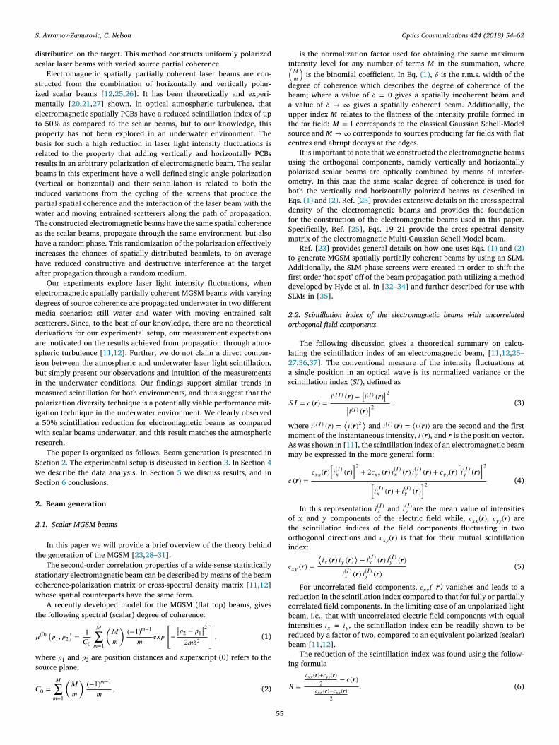
Fig. 2. Mean light intensity 𝐼𝑎𝑣𝑔 across the sensor area: (a) still conditions 𝑀𝐼𝑎𝑣𝑔 = 1 (units) with the standard deviation across the sensor area of 0.083 (units), (b)mechanically agitated (fast mode) conditions 𝑀𝐼𝑎𝑣𝑔 = 0.76 (units) with the standard deviation across the sensor area of 0.075 (units). The images are normalized tothe still condition values in order to show the spatial beam spread.

the light, 𝐼𝑎𝑣𝑔 from the electromagnetic MGSM beam with a coherencewidth, 𝛿, of 0.77 mm in still and mechanically agitated conditions (fastmode). It is apparent that the beam is visible at the middle of theimage, with some practical filtering artefacts. The objective of Fig. 2 is toshowcase that the overall beam spreading between experimental casesis not significant over the propagation path length of the experiment.The overall normalized intensity was reduced once the underwaterconditions became mechanically agitated. Assuming that each image,(im), is an m x n matrix, with 𝑚 = 480 and 𝑛 = 640, and that there are𝑁 = 1000, images taken we find the matrix 𝐼𝑎𝑣𝑔 as:

𝐼𝑎𝑣𝑔 =

∑𝑁𝑗=1(𝑖𝑚)𝑗𝑁

(7)

The image of 𝐼𝑎𝑣𝑔 serves as an insight into the beam quality at thetarget.

Additionally, to obtain an overall single value comparative param-eter, 𝑀𝐼𝑎𝑣𝑔 , the mean value of 𝐼𝑎𝑣𝑔 is calculated. 𝑀𝐼𝑎𝑣𝑔 represents thetotal ‘raw’ averaged intensity:

𝑀𝐼𝑎𝑣𝑔 =

∑𝑛𝑘=1

∑𝑚𝑗=1 𝐼𝑎𝑣𝑔𝑗,𝑘𝑛𝑚

(8)

The parameter 𝑀𝐼𝑎𝑣𝑔will be used to numerically compare the prop-agation of the laser beams in various underwater conditions.

The spatial variance of the laser light intensity fluctuations acrossthe sensor area with the background adjustment, 𝐵𝑎𝑣𝑔 , applied to eachimage is calculated as the scintillation index 𝑆𝐼𝐵 :

𝑆𝐼𝐵 =

∑𝑁𝑖=1

((

𝑖𝑚𝑖−𝐵𝑎𝑣𝑔)

−(𝐼𝑎𝑣𝑔−𝐵𝑎𝑣𝑔 ))2

𝑁

(𝐼𝑎𝑣𝑔 − 𝐵𝑎𝑣𝑔)2(9)

where 𝐵𝑎𝑣𝑔 is a single value parameter representing the average back-ground intensity.

To obtain a single parameter representing SI (see Eq. (3)) we findthe average value 𝑀𝑆𝐼𝐵𝑎𝑣𝑔

𝑀𝑆𝐼𝐵𝑎𝑣𝑔 =

∑𝑛𝑘=1

∑𝑚𝑗=1 𝑆𝐼𝐵𝑗,𝑘𝑛𝑚

(10)

Fig. 3 represents the scintillation index across the sensor in stilland fast moving mechanically agitated conditions. The increase inscintillation between Fig. 3a and Fig. 3b (going from 𝑀𝑆𝐼𝐵𝑎𝑣𝑔 = 0.059to 𝑀𝑆𝐼𝐵𝑎𝑣𝑔 = 0.08) is significant since the standard deviation of themeasurements across the whole sensor is low.

Fig. 4 shows a typical distribution of the scintillation index calcu-lated for each pixel, as a function of measured camera light intensity(non-normalized). The correlation between the low intensity camerameasurements and the calculated scintillation was observed. In orderto eliminate this dependence, the scintillation index for the intensitieslower than 1000 units were eliminated from the pool used for thecalculation of 𝑀𝑆𝐼𝐵𝑎𝑣𝑔 . That said, it is important to mention that themeasured trends reported do not change even if this precaution is notimplemented, due to the very high number of realizations used to derivestatistics (307,200). During the testing, the intensity of the light on thecamera sensor was kept constant (in the middle of the full camera range)by the use of neutral density filters. Additionally, we also selected onlya part of the sensor to test the dependency of the results on the locationof the beam on the sensor. Calculated scintillation trends for the cut-outsensor were exactly the same as for the whole sensor area. These variousanalysis steps were implemented in order to establish the reliability ofour observations.

57

S. Avramov-Zamurovic, C. Nelson Optics Communications 424 (2018) 54–62

Fig. 3. Scintillation index 𝑆𝐼𝐵 across the sensor area for MGSM coherence width, 𝛿, 0.77 mm: (a) still conditions 𝑀𝑆𝐼𝐵𝑎𝑣𝑔 = 0.059 with the standard deviationacross the sensor area of 0.0124, (b) mechanically agitated (fast mode) conditions 𝑀𝑆𝐼𝐵𝑎𝑣𝑔 = 0.08 with the standard deviation across the sensor area of 0.0074.

Fig. 4. Dependence of the scintillation index, 𝑆𝐼𝐵 , on the measured light intensity for the electromagnetic MGSM beam with coherence width, 𝛿, of 0.77 mm for themechanically agitated conditions (fast mode). Measured 𝑀𝑆𝐼𝐵𝑎𝑣𝑔 = 0.08 units with the standard deviation of 0.0074 units. Note, the total number of measurementswas 307,200.

58

S. Avramov-Zamurovic, C. Nelson Optics Communications 424 (2018) 54–62

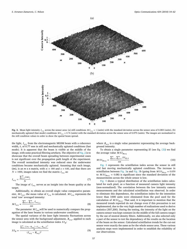
Fig. 5. Average light intensity 𝑀𝐼𝑎𝑣𝑔 measured across the sensor for stillconditions for each light polarization as a function of coherence width, 𝛿. Where,E beam is an electromagnetic beam, and V beam and H beam are vertically andhorizontally polarized scalar beams respectively.

5. Results

We present measured light intensities and their variations, and thescintillation index for spatially partially coherent beams with variedspatial coherence widths and polarization, and also Gaussian beams.

Note that, 𝛿 was defined in Eq. (1) as the r.m.s. width of the degreeof coherence and it is labelled coherence width in the figures. 𝛿 iscalculated from the SLM resolution and number of pixels used in theconstruction of the SLM screen and is described in [22].

5.1. Electromagnetic spatially partially coherent beams with flat top profile

Fig. 5 represents the scope of the experiments in terms of the MGSMbeam spatial coherence width sizes tested as well as relative intensityvalues recorded. The most significant feature is a linear increase inthe intensity as the beams become more coherent. The measurementsare shown in normalized units to the most spatially coherent E beam.Note that there are two measurements taken for a coherence width, 𝛿,size 0.77 mm due to the change in the number of screens cycled forthe coherence width radii 0.77 mm case. Seven of the measurementswere taken with 8000 phase screens and two sets with 2000 phasescreens (0.77 mm and the 1.09 mm cases), where the 0.77 mm caseoverlapped with the 8000 phase screens to show consistency in the datameasurements. Fig. 5 shows that the change in number of cycled screensdoes not influence the intensity measurements.

Fig. 6 shows that the measured intensity for vertically and horizon-tally polarized beams slightly differ as a function of coherence width.The trend is similar between still and agitated conditions, with thelarger differences showing for the less spatially coherent beams, andmore agreement when more spatially coherent beams are propagated.While this difference should have remained constant over the scope ofexperimentation, it has to be taken into the consideration that there wasa slight mismatch between the vertical and horizontal scalar beams assuggested using the polarimeter. That said the measurements in Fig. 6suggest a possible dependence of the measured intensity on the spatialcoherence of the beam.

Fig. 7 shows measured 𝑀𝑆𝐼𝐵𝑎𝑣𝑔 for typical agitated conditions, andTable 2 summarizes the effect of polarization on scintillation in terms ofhow much the scintillation is decreased when the intensity fluctuationsfor scalar and electromagnetic beams are compared. Measured reduc-tion, MR, as given in Table 2, and is based on actual measurements ofthe scintillation of the electromagnetic beam 𝑀𝑆𝐼𝐵𝑎𝑣𝑔𝐸𝑏𝑒𝑎𝑚 , and thescalar beams 𝑀𝑆𝐼𝐵𝑎𝑣𝑔𝑉 𝑒𝑟𝑡𝑖𝑐𝑎𝑙 and 𝑀𝑆𝐼𝐵𝑎𝑣𝑔𝐻𝑜𝑟𝑖𝑧𝑜𝑛𝑡𝑎𝑙:

𝑀𝑅 =𝑀𝑆𝐼𝐵𝑎𝑣𝑔𝑉 𝑒𝑟𝑡𝑖𝑐𝑎𝑙+𝑀𝑆𝐼𝐵𝑎𝑣𝑔𝐻𝑜𝑟𝑖𝑧𝑜𝑛𝑡𝑎𝑙

2 −𝑀𝑆𝐼𝐵𝑎𝑣𝑔𝐸𝑏𝑒𝑎𝑚𝑀𝑆𝐼𝐵𝑎𝑣𝑔𝑉 𝑒𝑟𝑡𝑖𝑐𝑎𝑙+𝑀𝑆𝐼𝐵𝑎𝑣𝑔𝐻𝑜𝑟𝑖𝑧𝑜𝑛𝑡𝑎𝑙

2

(11)

Fig. 6. Measured intensity difference between the vertically and horizontallypolarized light, as a function of coherence width in (a) still, and (b) mechanicallyagitated conditions. Note, a red labelled data point outlier in Fig. 6a. (Forinterpretation of the references to colour in this figure legend, the reader isreferred to the web version of this article.)

Eq. (4) gives a method to calculate the SI for the electromagneticbeam in atmospheric turbulence based on the intensity and the scintil-lation of the scalar beams and thus reduction given in Eq. (6) dependsonly on the scalar beam performance. Eq. (11) uses the measured SI forboth scalar and electromagnetic beams.

The significance of this result is that we have experimentally mea-sured about a 50% reduction for the beams propagating underwater instill conditions and about a 40% reduction in agitated conditions. Thisfinding demonstrates the possibility to use the polarization diversity formitigating some of the deterioration effects on laser light propagationin an oceanic environment. Interestingly, in still water the reduction inscintillation is consistent and more closely follows the theory derivedfor the spatially PPCBs propagating in atmospheric optical turbulence.Measured scintillation in mechanically agitated water does not onlydepend on imperfection in electromagnetic beam generation due tothe finite SLM cycling rate, but also potentially on some multi-pathpropagation created by moving entrained scatterers. As a consequence,the scintillation index is generally higher in mechanically agitatedwater, and the observed scintillation reduction is less.

Fig. 8 shows the standard deviation of the 𝑀𝑆𝐼𝐵𝑎𝑣𝑔 measurementsand it demonstrates the confidence in the presented results. Based on themeasurement uncertainty as demonstrated with the standard deviationvalues, it is possible to confidently estimate the performance trends fromour results.

Fig. 9 shows the comparison of 𝑀𝑆𝐼𝐵𝑎𝑣𝑔 for the still and me-chanically agitated conditions with mechanically agitated fast movingentrained scatterers. Note the match in the performance of both scalarbeams in respective conditions. Measurements clearly show a substan-tial reduction in scintillation on the order of 50% when scalar beams arecompared to the electromagnetic beams for the full range of coherencewidth values and water conditions.

Fig. 10 shows the ratio between the scintillation in agitated con-ditions and still conditions. The ratio shows how much stronger the

59

S. Avramov-Zamurovic, C. Nelson Optics Communications 424 (2018) 54–62

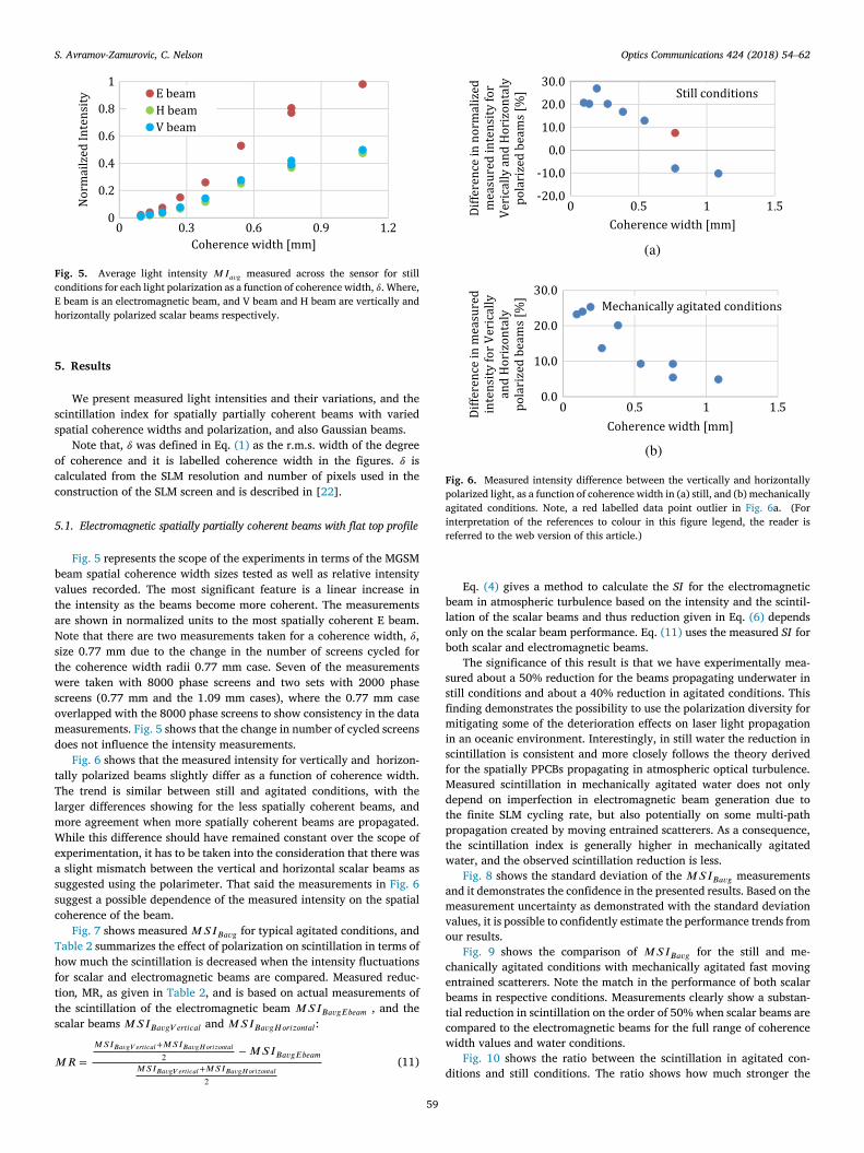
Table 2Dependence of measured and estimated scintillation index reduction on coher-ence width in PPCBs.

Widthradius[mm]

MeasuredreductionMR (Eq. (11))Still[%]

EstimatedreductionR (Eq. (6))Still[%]

MeasuredreductionMR Eq. (11)Agitated[%]

EstimatedreductionR Eq. (6)Agitated[%]

0.096 49 49 43 500.136 49 49 39 500.192 50 49 44 490.271 50 50 43 490.384 48 50 41 500.543 50 50 39 480.768 47 50 37 490.768a 50 50 39 491.085a 45 50 35 50

Note: Agitated conditions are with mechanically agitated fast moving scatterers.a Change in number of cycling screens on SLM from 8000 to 2000 phase

screens.

Fig. 7. Measured average scintillation index, 𝑀𝑆𝐼𝐵𝑎𝑣𝑔 in agitated conditions(with slow moving scatterers). Note the lower values for the electromagneticbeams and matched higher values for the scalar beams polarized vertically andhorizontally. The * denotes the change in number of cycling screens on SLMfrom 8000 to 2000 phase screens.

Fig. 8. Measured 𝑀𝑆𝐼𝐵𝑎𝑣𝑔 across the sensor area for electromagnetic beampropagating in still conditions with one standard deviation upper and lowerconfidence interval bounds.

scintillation is in a more complex media; but its trend also demonstratesan increase in scintillation for more spatially coherent beams relativeto less spatially coherent beams. This ratio is around 1 for less spatiallycoherent beams, increasing to 1.5 as the beam becomes more spatiallycoherent. Note that the scalar beams are increasingly more proneto scintillation as they become more coherent. The deterioration ofelectromagnetic PPCB beams is less volatile.

If the scintillations in slow and fast moving entrained scattererconditions are compared, the clear increase in scintillation in a morecomplex media is apparent. It should be noted that the construction ofPPCBs through the use of the cycling of statistically prescribed phase

Fig. 9. Measured 𝑀𝑆𝐼𝐵𝑎𝑣𝑔 , comparison between the still condition and the fastmoving scatterers condition as a function of coherence width values, for scalar(horizontally and vertically polarized) and electromagnetic beams.

Fig. 10. The ratio between the fast moving scatterers condition and thestill condition of 𝑀𝑆𝐼𝐵𝑎𝑣𝑔 , as a function of coherence width, 𝛿, for scalar(horizontally and vertically polarized) and electromagnetic beams.

screens with the SLM introduces additional fluctuations in the laserlight on the target. As noted, theoretically, the cycling rate is infinite,but practically we have hardware limitations in cameras capture rateand SLM cycling rate and these instrumentation restrictions are theprimary influence on the scintillation values in the still conditions.It can be observed that scintillations in the still conditions and themechanically agitated condition where the scatterers are moving slowlyare comparable in values. The reason for this effect for slow mode, isthat light intensity variations due to the SLM cycling rate are dominantin comparison to the constructive and destructive interference due tothe light interacting with the moving scatterers.

5.2. Gaussian beam

To evaluate the performance of a coherent, Gaussian laser beam,six sets of experiments were recorded: three under the still conditionsand three in mechanically agitated (fast moving entrained scatterers)conditions.

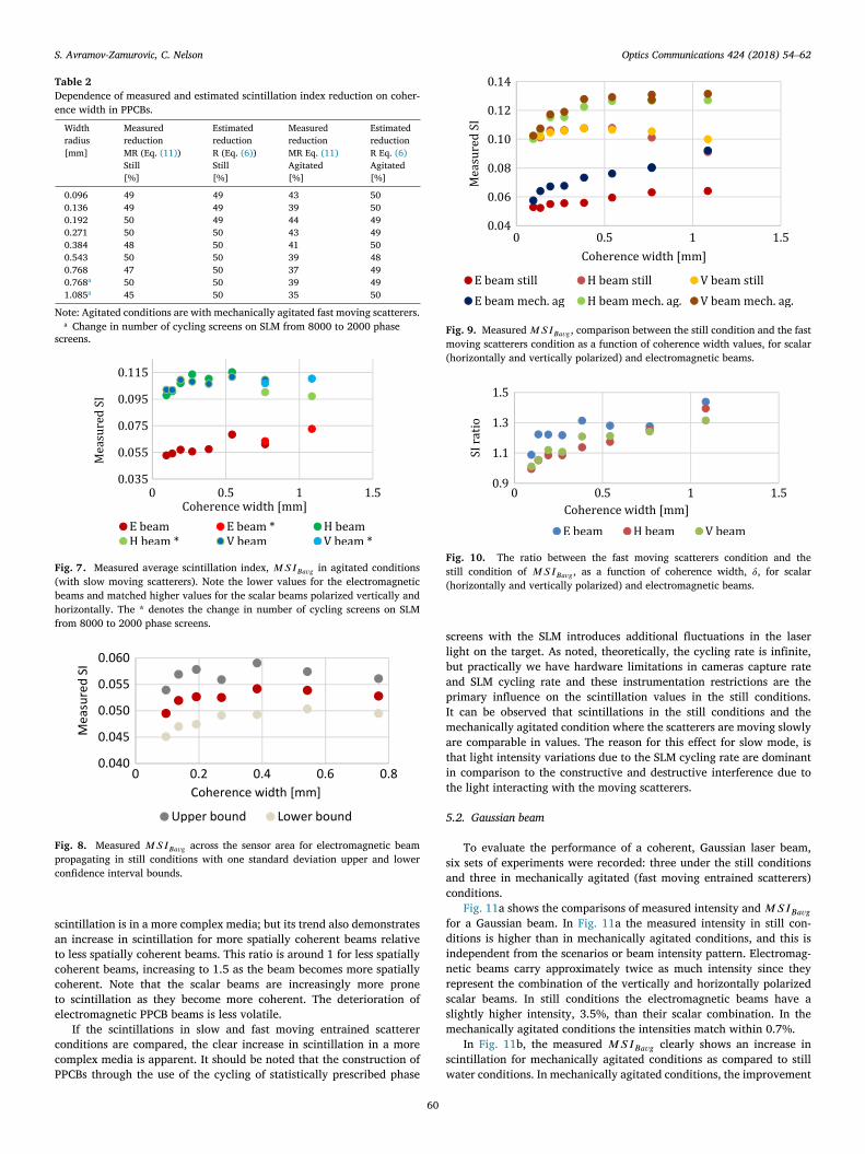
Fig. 11a shows the comparisons of measured intensity and 𝑀𝑆𝐼𝐵𝑎𝑣𝑔for a Gaussian beam. In Fig. 11a the measured intensity in still con-ditions is higher than in mechanically agitated conditions, and this isindependent from the scenarios or beam intensity pattern. Electromag-netic beams carry approximately twice as much intensity since theyrepresent the combination of the vertically and horizontally polarizedscalar beams. In still conditions the electromagnetic beams have aslightly higher intensity, 3.5%, than their scalar combination. In themechanically agitated conditions the intensities match within 0.7%.

In Fig. 11b, the measured 𝑀𝑆𝐼𝐵𝑎𝑣𝑔 clearly shows an increase inscintillation for mechanically agitated conditions as compared to stillwater conditions. In mechanically agitated conditions, the improvement

60

S. Avramov-Zamurovic, C. Nelson Optics Communications 424 (2018) 54–62

Fig. 11. Gaussian beam measurements in still and turbid conditions withmechanically agitated fast moving scatterers: (a) Measured intensity 𝑀𝐼𝑎𝑣𝑔 and(b) Measured scintillation 𝑀𝑆𝐼𝐵𝑎𝑣𝑔 .

when an electromagnetic beam is used as compared to the scalar beamgives on average 17% in scintillation reduction. If we observe each run,the reduction is 17%, 12%, and 22% respectively, and these variationsin the measurements are primarily due to the random motion of thescatterers with variable diameters moving in the water. It is significantto point out that the reduction in scintillation is not on the order of 50%as measured for PPCB. When a Gaussian beam is propagated in stillconditions the reduction in scintillation is not significant, suggestingthat since the measured scintillation is so low, that the benefit ofpropagating electromagnetic versus scalar beam is not observable.

For the electromagnetic beam, when the average measured scin-tillation in still water, 0.013, is compared to the average scintillationin mechanically agitated water, 0.043, the performance is 3.3 timesworse in the more complex medium. In the case of scalar beams,the performance deterioration in the mechanically agitated conditionis even more significant: measured 𝑀𝑆𝐼𝐵𝑎𝑣𝑔 on average going from0.0099 in still conditions to 0.051 in mechanically agitated water, withthe SI ratio being 5.1.

When the same performance metrics are compared for the fully co-herent, Gaussian, electromagnetic beam (scintillation ratio from still tomechanically agitated conditions of 3.3) and electromagnetic spatiallypartially coherent beams (1.5) the trend strongly benefits the PPCBs.

6. Conclusions

We investigated the propagation of polarized spatially partially co-herent and fully coherent Gaussian, laser beams underwater under twoconditions: still water and mechanically agitated water with entrainedscatterers.

In the case of the spatially partially coherent beams, the reduc-tion in scintillation from propagating a scalar beam to propagatingan electromagnetic beam was measured to be approximately 50%reduction in scintillation in less complex media (still water), but theperformance was at the level of 40% reduction in scintillation in morecomplex environments (water with mechanically moving scatterers). Wemeasured a 17% reduction in scintillation when fully coherent scalar,

Gaussian, and electromagnetic coherent beams are compared in morecomplex underwater media. In still conditions measured scintillationsfor the coherent beams was very low, and therefore the measurementuncertainty prevented a good estimate of the scintillation reduction forthis case.

Furthermore, it was observed that the less coherent spatially partiallycoherent beams have better scintillation reduction performance as com-pared with more coherent beams, propagating underwater. In general,depending on the coherence width value of a partially coherent beams,the beam spreading is wider as compared to the Gaussian beam, but ifthe loss of the power could be normalized, the scintillation performanceof the partially coherent beams appears superior.

We also established that the Gaussian beam scintillation deterioratesmore rapidly as the medium becomes more complex, as compared to thespatially partially coherent beams under the same conditions underwa-ter. It is important to note that spatially partially coherent beams havean initial intensity fluctuation due to the construction of the beam usinga cycling spatial light modulator. Those induced variations are uniformacross the beam cross section and become relatively negligible whenlaser light is propagated through a highly turbulent medium.

Acknowledgements

S. Avramov-Zamurovic is supported by US ONR grant: N0001414-WX-00267.C. Nelson is supported by US ONR grant N0001416WX00796.

References

[1] L.C. Andrews, R.L. Phillips, Laser Beam Propagation Through Random Media, seconded., SPIE Press, Bellingham, WA, 2005.

[2] A. Ishimaru, Wave Propagation and Scattering in Random Media, Vols. 1 and 2,Academic, San Diego, Calif., 1978.

[3] F. Wang, X. Liu, Y. Cai, Propagation of partially coherent beam in turbulentatmosphere: a review (invited review), Prog. Electromagn. Res. 150 (2015) 123–143.

[4] V.A. Banakh, V.M. Buldakov, Effect of the initial degree of spatial coherence of alight beam on intensity fluctuations in a turbulent atmosphere, Opt. Spectrosc. 55(1983) 707–712.

[5] J.C. Ricklin, F.M. Davidson, Atmospheric turbulence effects on a partially coherentgaussian beam: implications for free-space laser communication, J. Opt. Soc. Amer.A 19 (2002) 1794–1802.

[6] J.H. Churnside, Aperture averaging of optical scintillations in the turbulent atmo-sphere, Appl. Opt. 30 (1991) 1982–1994.

[7] S. Rosenberg, M.C. Teich, Photocounting array receivers for optical communicationthrough the lognormal atmospheric channel 2: optimum and suboptimum receiverperformance for binary signaling, Appl. Opt. 12 (1973) 2625–2634.

[8] E.J. Lee, V.W.S. Chan, Part 1: optical communication over the clear turbulentatmospheric channel using diversity, IEEE J. Sel. Areas Commun. 22 (2004) 1896–1906.

[9] G.P. Berman, A.R. Bishop, B.M. Chernobrod, D.C. Nguyen, V.N. Gorshkov,Suppression of intensity fluctuations in free space high-speed optical communicationbased on spectral encoding of a partially coherent beam, Opt. Commun. 280 (2007)264–270.

[10] G.P. Berman, A.A. Chumak, Influence of phase-diffuser dynamics on scintillationsof laser radiation in Earth’s atmosphere: long-distance propagation, Phys. Rev. A 79(2009) 063848–063854.

[11] O. Korotkova, Scintillation index of a stochastic electromagnetic beam propagatingin random media, Opt. Commun. 281 (2008) 2342–2348.

[12] Y. Gu, O. Korotkova, G. Gbur, Scintillation of nonuniformly polarized beams inatmospheric turbulence, Opt. Lett. 34 (2009) 2261–2263.

[13] X. Xiao, D. Voelz, Wave optics simulation of partially coherent and partiallypolarized beam propagation in turbulence, in: Proc. SPIE 7464, Free-Space LaserCommunications IX, 74640T, Aug 21, San Diego, CA, 2009.

[14] F. Schill, U.R. Zimmer, J. Trumpf, Visible spectrum optical communication anddistance sensing for underwater applications, in: Proc. Australasian Conf. Robot.Autom., 2004.

[15] N. Farr, J. Ware, C. Pontbriand, T. Hammar, M. Tivey, Optical communicationsystem expands CORK seafloor observatory’s bandwidth, in: Proc. OCEANS Conf.,2010.

[16] M. Doniec, C. Detweiler, I. Vasilescu, D. Rus, Using optical communication forremote underwater robot operation, in: IEEE/RSJ International Conference onIntelligent Robots and Systems, 2010.

61

S. Avramov-Zamurovic, C. Nelson Optics Communications 424 (2018) 54–62

[17] B. Cochenour, A. Laux, L. Mullen, Temporal dispersion in underwater laser com-munication links: Closing the loop between model and experiment, in : ProceedingsUnderwater Communications and Networking Conference (UComms), IEEE Third,2016.

[18] O. Korotkova, N. Farwell, E. Shchepakina, Light scintillation in oceanic turbulence,Waves Random Complex Media 22 (2) (2012) 260–266.

[19] Y. Wu, Y. Zhang, Y. Zhu, Average intensity and directionality of partially coherentmodel beams propagating in turbulent ocean, J. Opt. Soc. Am. A 33 (8) (2016) 1451–1458.

[20] S. Avramov-Zamurovic, C. Nelson, S. Guth, O. Korotkova, R. Malek-Madani,Experimental study of electromagnetic Bessel-Gaussian Schell Model beams prop-agating in a turbulent channel, Opt. Commun. 359 (2016) 207–215.

[21] S. Avramov-Zamurovic, C. Nelson, R. Malek-Madani, O. Korotkova, Polarization-induced reduction in scintillation of optical beams propagating in simulated turbu-lent atmospheric channels, Waves Random Complex Media 24 (4) (2014) 452–462.

[22] S. Avramov-Zamurovic, O. Korotkova, C. Nelson, R. Malek-Madani, The dependenceof the intensity PDF of a random beam propagating in the maritime atmosphere onsource coherence, Waves Random Complex Media 24 (2014) 69–82.

[23] O. Korotkova, S. Sahin, E. Shchepakina, Multi-Gaussian schell-model beams, J. Opt.Soc. Am. A 29 (2012) 2159–2164.

[24] D. Voelz, K. Fitzhenry, Pseudo-partially coherent beam for free-space laser commu-nication, Proc. SPIE 5550 (2004) 218–224.

[25] Z. Mei, O. Korotkova, E. Shchepakina, Electromagnetic multi-gaussian schell-modelbeams, J. Opt. 15 (2013) 025705.

[26] T. Shirai, O. Korotkova, E. Wolf, A method of generating electromagnetic GaussianSchell model beams, J. Opt. A: Pure Appl. Opt. 7 (2005) 232–237.

[27] A.S. Ostrovsky, G. Rodríguez-Zurita, C. Meneses-Fabián, M.Á. Olvera-Santamaría,C. Rickenstorff-Parrao, Experimental generating the partially coherent and partiallypolarized electromagnetic source, Opt. Express 18 (2010) 12864–12871.

[28] E. Wolf, Unified theory of coherence and polarization of random electromagneticbeams, Phys. Lett. A 312 (2003) 263–267.

[29] G. Gbur, T.D. Visser, The structure of partially coherent fields, Prog. Opt. 55 (2010)285.

[30] F. Gori, Matrix treatment for partially polarized, partially coherent beams, Opt. Lett.23 (1998) 241–243.

[31] S. Sahin, O. Korotkova, Light sources generating far fields with tunable flat profiles,Opt. Lett. 37 (2012) 2970–2972.

[32] M.W. Hyde IV, S. Basu, X. Xiao, D. Voelz, Producing any desired far-field meanirradiance pattern using a partially-coherent schell-model source, J. Opt. 17 (2015)055607.

[33] M.W. Hyde, S. Basu, X. Xiao, D.G. Voelz, Producing any desired far-field meanirradiance pattern using a partially-coherent Schell-model source and phase-onlycontrol, Imaging and Applied Optics 2015 OSA Technical Digest (online) (OpticalSociety of America), paper PW3E.2. (2015).

[34] M.W. Hyde, S. Basu, D.G. Voelz, X. Xiao, Experimentally generating any desiredpartially coherent schell-model source using phase-only control, J. Appl. Phys. 118(2015) 093102.

[35] S. Avramov-Zamurovic, C. Nelson, S. Guth, O. Korotkova, Flatness parameter influ-ence on scintillation reduction for multi-Gaussian Schell-model beams propagatingin turbulent air, App. Opt. 55 (13) (2016) 3442–3446.

[36] Y. Baykal, H.T. Eyyuboğlu, Y. Cai, Scintillations of partially coherent multipleGaussian beams in turbulence, App. Opt. 48 (10) (2009) 1943–1954.

[37] C. Mujat, A. Dogariu, Statistics of partially coherent beams: a numerical analysis, J.Opt. Soc. Amer. A 21 (6) (2004) 1000–1003.

[38] E. Hecht, Optics, fourth ed., Pearson Addison Wesley, 2002.[39] S. Avramov-Zamurovic, C. Nelson, Experimental study on off-axis scattering of flat

top partially coherent laser beams when propagating under water in the presence ofmoving scatterers, Waves in Random and Complex Media, 2017.

[40] S. Avramov-Zamurovic, C. Nelson, Experimental analysis of laser beams withvariable spatial coherence propagating underwater. In: Imaging and Applied Optics2017 (3D, AIO, COSI, IS, MATH, pcAOP), OSA Technical Digest (online) (OpticalSociety of America, paper PTh1D.3, 2017.

[41] C. Nelson, S. Avramov-Zamurovic, O. Korotkova, S. Guth, R. Malek-Madani,Scintillation reduction in pseudo Multi-Gaussian Schell Model beams in the maritimeenvironment, Opt. Commun. 364 (2016) 145–149.

62