EXPERIMENTS INMODERN PHYSICSSecond Edition

Adrian C. MelissinosUNIVERSITY OF ROCHESTER

Jim NapolitanoRENSSELAER POLYTECHNIC INSTITUTE

@ACADEMIC PRESSAn imprint of Elsevier Science

Amsterdam Boston London New York Oxford Paris San DiegoSan Francisco Singapore Sydney Tokyo

2.3 Experiment on the Hall Effect 63

The main source of systematic uncertainty is likely to come from thetimes over which the decaying voltage signal is fitted. At short times, thedecay is not a pure exponential because the transient terms have not alldied away, so we want to exclude these times when we fit. At long times,there may be some left over voltage level that is a constant added to theexponential , and again, a pure exponential fit will be wrong. Varying theupper and lower fit limits until we get a set that gives the same answer asa set that is a little bit larger on both ends is one approach. One should beconvinced that the results are consistent. For example, use aluminum alloyrods of the same composition but different radii, and check to make surethat the decay lifetimes tE scale like r 2. This should certainly be the caseto within the estimated experimental uncertainty.

Having learned how to take and analyze data on resistivity, we can nowinvestigate the temperature dependence. It is best to start simply by com­paring the two samples of ~-in. diameter aluminum rods, one an alloy andthe other a (relatively) pure metal. Vary the temperature by immersing thesamples in baths of ice water, dry ice and alcohol, and liquid nitrogen.Boiling water or hot oil can also be used. These measurements are tricky.One must remove the sample from the bath and measure the eddy currentdecay before the temperature changes very much. Probably the best way todo this is to take a single trace right after inserting the sample, stop the oscil­loscope, and store the trace . Then one analyzes the trace offline to get thedecay constant. One might also try to estimate how fast the bar warm s up bymaking additional measurements after waiting several seconds, e.g. , aftersaving the trace . This would best be done with a sample whose resistivity,and therefore tE, can be expected to change a lot with temperature. Purealuminum is a good choice. Remember that the temperature dependencewill be much different for the pure metal than for the alloy. Try to estimatethe contribution to the mean free path of the electrons due to the impurities.

2.3. EXPERIMENT ON THE HALL EFFECT

In Section 2.2 we saw how colli sions of electrons with the crystal latticelead to an electrical resistance, when those electrons are forced to moveunder an electric field. If one also applie s a magnetic field, in a directionperpendicular to the electric field, then the electrons (and other currentcarriers) will be deflected sideways. As a result an electric field appears inthis direction, and therefore also a potential difference. This phenomenon

64 2 Electrons in Solids

is called the Hall effect, and has important applications both in identifyingthe current carriers in a material and for practical use as a technique formeasuring magnetic fields.

Let us rewrite the microscopic formula for Ohm's law, but this timetaking care to indicate current density and electric fields as vectors, andto also note the negative sign of the charge on the electron. FollowingEqs. (2.12) and (2.13) we write

orIllVd-- = -eE.

r

(2.18)

(2.19)

It is clear that in Eq. (2.19) we have made an approximation, replacingthe time rate of change of momentum, i.e., dpjdt = mdvjdt, with anexpression that uses the average acceleration vdjr. This is how we havetaken into account collisions with the crystal lattice.

It is straightforward to modify Eq. (2.19) to take into account the effectof a magnetic field B. We have

mVd- = - e(E+vd x B).r

If we assume that the magnetic field lies in the z direction, and define thecyclotron frequency We == eB j m, then we can rewrite this equation as

erVdx = --Ex - WerVdy

IIIer

Vd . = --Ey + WerVdx)' III

erVd = - -Ez ·

l III

(2.20)

Consider now a long rectangular section of a conductor, as shown inFig . 2.13. A longitudinal electric field Ex is applied, leading to a currentdensity flowing in the x direction. As this electric field is initially turnedon, the magnetic field deflects electrons along the y direction. This leads toa buildup of charge on the faces parallel to the xz plane, and therefore anelectric field E y within the conductor. In the steady state, this electric fieldcancels the force due to the magnetic field, and the current density is strictly

2.3 Experiment on the Hall Effect 65

Magnetic field 8 2

t t t t t

-Ex+ + + + + + + +

(2.21)

(a)

Sectionperpend icular

to z axis;drift velocity

just starting up. L-..........Ii:I5 ........__......_ llE................

(b)

Sect ionperpendicular

to z axis ;drift veloc ity

in steady state . 1..- .:.......;:...- ----1

(c)

FIGURE 2. 13 The standard geometry for discussing the Hall effect (after Kittel).

in the x direction, hence Vdy = O. From Eqs. (2.20) we therefore have

mco; mco; ( er ) e B rEy = --Vd = -- --Ex = -wcr Ex = ---Ex.

e x e m m

The appearance of the electric field Ey is the Hall effect.A convenient experimental quantity is the Hall coefficient RH, defined as

EyRH=-

j x B

The quantities E y , jx, and B are all straightforward to measure , and in oursimple approximation for electrons in conductors we have (from Eq. (2.18))j x = ne2r E.dm; therefore,

e B't Ex/mRH = ---;:;-----'---­

(ne2r Ex/m )B ne(2.22)

66 2 Electrons in Solids

That is, the Hall coefficient is the inverse of the carrier charge density. Infact, the Hall effect is a useful way to measure the concentration of chargecarriers in a conductor. It is also convenient to define the Hall resistivity asthe ratio of the transverse electric field to the longitudinal current density,that is,

PH == Ey/jx = BRH, (2.23)

which depends (in our approximation) only on the material and the appliedmagnetic field.

2.3.1. Measurements

In order to measure the Hall effect, one needs a sample of a conductor,but not an especially good conductor. This is because one also needs arelatively low carrier density ne in order to get a sizable effect; this ofcourse leads to a relatively high resistivity. As seen in Table 2.1, bismuthis a good candidate metal, and we describe such an experiment here. II

The setup uses a bismuth sample with rectangular cross section, mountedon a probe with attached leads for measuring current and voltage. A ther­mocouple is also attached to the sample so that temperature measurementscan be carried out. The magnetic field is provided by an electromagnetcapable of delivering a field up to "'5 kG over a volume roughly 1 crrr'.The bismuth sample probe is shown in Fig. 2.14. The width of the bismuthsample is w = 6.5 mm and its thickne ss, measured with a micrometer,is t = 1.65 x 10- 4 m. The effective length of the sample is the distancebetween the leads used to measure the current ("white" and "brown," asshown in Fig. 2.14). In our case, this distance is e = 7 mm. Current issupplied by a DC power supply, connected to the sample through the "red"and "black" leads. The Hall voltage is measured with a digital multimeter,using the "green" lead and the output of a potentiometer used to balancethe voltage on the "white" and "brown" leads. A separate bundle of wiresare connected to leads that carry current to the heating resistor, and to athermocouple that measure s the temperature of the bismuth sample.

Begin by determining the Hall coefficient at room temperature and for arelatively high magnetic field. Tum on the electromagnet power supply to

II Semiconductors also make good candidates, with a very low carrier density comparedto a metal. For a description of such a setup, see A. Melissinos, Experiments ill ModernPhysics , First ed., Academic Press, New York, 1966.

2.3 Exper iment on the Hall Effect 67

While

Brown

CUfl\ II

~b"White

I IBrown

Black 10 \ Il.......--e -..I r IBi : I :, ,

-jGreen --

Red 4III

AI I AIII ~

Cu

Black

•~f--ReS_istor ~

FIGURE 2.14 Schematic of the probe used to make measurements of the Hall effec tin bismuth. Electrica l connectio ns are made to the bismuth sample using copper leads. Athermocouple, as well as a resistor which acts as a heat source, is also attached to the sample.Two separa te bundles of wires emerge from the probe, one of which is used exclusively forheating the sample and for measuring its temperature.

around 4 kG. It will likely need an hour or so to stabilize. In the meantime,with the sample probe removed from the magnetic field , run about 3 Athrough the bismuth sample, and adjust the potentiometer so that the Hallvoltage is zero . Return the current through the sample to ze ro . The samplecan get quite hot while it is conducting so much current. Be caref ul not totouch it, or to touch it to anything else.

When the electromagnet is stabilized, measure and record the magneticfield us ing a gaussmeter, or by some other technique. Now, place the sampleprobe in the center of the magnetic field . Quickly rai se the current I throughthe sample to 3.0 A, and record the Hall voltage VH . Then, quickly, reducethe current by 0.25 A, and record the Hall voltage again. You should carrythis series of measurements out rather rapidly to avoid leaving the bismuthsample at high temperature for any extended period of time. When youhave reduced the current to near zero, and recorded the final value of the

68 2 Electrons in Solids

4r-- -..-- -..---,----,-------,,-------,r--7l

3.5

3 Slope=1.23 mV/A

30.5 1 1.5 2 2.5

Current through sample (A)

FIGURE 2.15 Sample of Hall effect data, taken at room temperature and with a magneticfield B = 4.42 kG

>.s 2.5

Q)Cl2:l 2(5>

'iiiI

0.5

Hall voltage , remove the probe and recheck the value of the magneticfield.

A sample of data taken in this way, at room temperature and with B =4.42 kG, is shown in Fig. 2.15. A free linear straight line fit gives a slopeof 1.23 mY/A, with an intercept very close to zero. In terms of quantitiesrelated to our measurement, the Hall coefficient (Eq. (2.21» is expre ssed by

e, VH/w VHt dVH tRH == - = - - - ---,

jx B II (w x t )B I B dI B

where we note that our data yields a very good direct proportionalrelationship between VH and I . Using SI units, this yields

RH = (1.23 x10- 3 V) (1.65 x10-4 m) = 4.59 x10-7 m3/C

A 0.442 T

This is quite close to an accepted room temperature value of RH = 5.4 x10- 7 m3/C for pure bismuth metal. The uncertainties in measuring thedimen sions of the sample can easily account for the discrepancy.

Of course, this sample and this setup can be used to determine theresistivity of bismuth. Outside of the magnetic field, measure the voltage

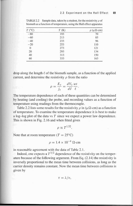
2.3 Experiment on the Hall Effect 69

TABLE 2.2 Sample data, taken by a student, for the resistivity p ofbismuth as a function of temperature, using the Hall effect appara tus

-80-60-40- 20o204060

T (K)

1932 132332532732933 13333

p (I.l Q-cm)

708596

110121134150163

drop along the length eof the bismuth sample, as a function of the appliedcurrent, and determine the resistivity p from the ratio

Ex dVx wtP=-. = dI T'

Jx

The temperature dependence of each of these quantities can be determinedby heating (and cooling) the probe , and recording values as a function oftemperature using readings from the thermocouple.

Table 2.2 lists some results for the resistivity p in ([.L Q-cm) as a functionof temperature. To examine the temperature dependence it is best to makea log-log plot of the data vs T since we expect a power law dependence.This is shown in Fig. 2.16 and when fitted gives

p ex T 1.52 .

Note that at room temperature (T = 25°C)

p = 1.4 X 10- 4 Q-cm

in reasonable agreement with the data of Table 2.1.Indeed, one expects a T 3/ 2 dependence of the resistivity on the temper­

ature because of the following argument. From Eq. (2.14) the resistivity isinversely proportional to the mean time between collisions, as long as thecarrier density remains constant. Now the mean time between collisions isgiven by

r = A/V,

70 2 Elee t ron sin Sol ids

•

p (25°C) = 139 (fin-em)

102.4

Temperature T (K)

FIGURE 2.16 The resistivity of bismuth as a function of tempe rature, taken with the Halleffect apparatus (data from Table 2.2.) The data are fitted to a power law form.

where A is the mean free path for scattering, and v the thermal velocity ofthe electrons. For v we can use

1 2 3-mv = -kT2 2

or v = J3kT/m.

The mean free path, A, decreases as the collision cross section increases,namely as the lattice vibrations increase with temperature. It is found thatA is inverse ly proportional to the temperature, and therefore

T ex I/T3/ 2

or using Eq. (2.14),

pexT3/ 2 .

We can also examine the temperature dependence of the Hall coeffi­cient. In this case it is best to plot RH on a semi-log plot vs 1/ T. Thereason is that the Hall coefficient (see Eq. (2.22)) is directly inversely pro­portional to the carrier density, and we expect the carrier density to dependon the temperature by an exponential factor, such as for instance shownin Eq, (2.28). The data are plotted in this way in Fig. 2.17, and we recog­nize two distinct slopes. As expected, RH falls with increasing temperature

2.4 Semiconductors 71

:0-E 10°·8o:;o

J,2E

2 2.5 3 3.5

1/T(K)

4 4.5 5x 10- 3

FIGURE 2. 17 Measurements of the Hall coefficient as a function of temperature.

because the carrier density increases. By fitting the data to the form

n ex exp(-E/2kT) ,

we find for the two region s

low T ,high T,

E = 0.029 eVE = 0.120 eV.

Such energy differences are typical of the excitation of impurities. It isalso relevant to note that the carrier density at room temperature is

n = l / eRH = 1.35 x 1019 cm- 3.

This is quite high and typical of a conductor.

2.4. SEMICONDUCTORS

2.4.1. General Properties of Semiconductors

We have seen in the first section how a free-electron gas behaves, and whatcan be expected for the band structure of a crystalline solid . In the second