+ All Categories
Home > Documents > Experiments were conducted in the University of Delaware’s ...

Experiments were conducted in the University of Delaware’s ...

Date post: 24-Jan-2022
Category:
Upload: others
View: 2 times
Download: 0 times
Share this document with a friend
10
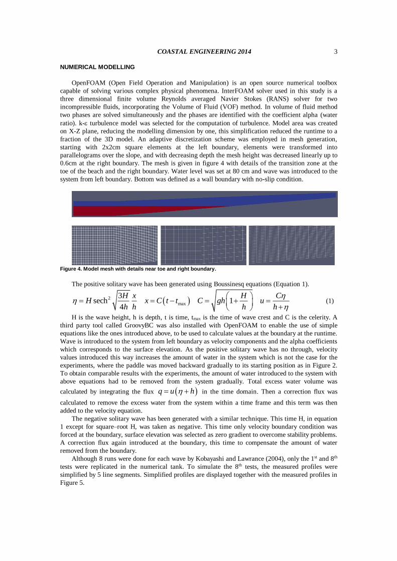
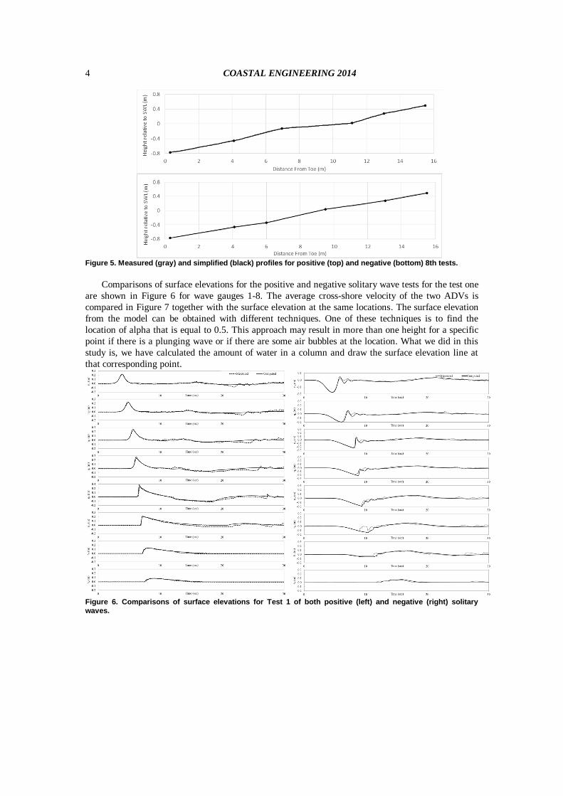
1 BREAKING OF POSITIVE AND NEGATIVE SOLITARY WAVES Burak Aydogan 1 and Nobuhisa Kobayashi 2 Surf dynamics of positive and negative solitary waves on a sandy beach are examined through physical modeling and numerical simulations to improve the quantitative understanding of wave runup and rundown caused by two different initial tsunami waves. Physical model tests of Kobayashi and Lawrance (2004) are replicated in a numerical 2D flume. We have used InterFOAM, a three dimensional, two phase, RANS solver, which is a part of OpenFOAM modelling library, in order to obtain the detailed spatial and temporal variations of the free surface elevation and velocity. Keywords: positive solitary wave; negative solitary wave; OpenFOAM modeling INTRODUCTION The knowledge on cross-shore sediment transport process of beaches under different kinds of tsunami waves is very scarce when compared to studies of sediment transport under wind waves. Kobayashi and Lawrance (2004) had done a series of experiments to fill that gap. Two experiments were conducted each consisting of 8 runs. One for positive solitary waves and one for negative solitary waves. Each run in an experiment was cumulative over the previous runs. Beach morphology surface elevations, sediment concentrations and ADV measurements were recorded for each test. Although valuable data recorded during the runs they weren’t enough to completely define the hydrodynamics and so the sediment transport mechanisms under these waves. So a numerical study was done to increase the understanding of hydrodynamics under positive and negative solitary waves. EXPERIMENTS (Lawrance and Kobayashi (2004)) Experiments were conducted in the University of Delaware’s wave flume which is 30m long, 2.4m wide and 1.5m height. A piston type wave generator was used to generate solitary waves. The water depth was 0.8m and a fine-sand beach was installed with an initial slope of 1/12. (Figure 1) The piston trajectory was computed using the method by Goring (1978) for the positive solitary wave tests. The wave paddle was moved backward slowly and then forward rapidly to generate the solitary wave. The paddle was then moved back to the original position slowly. For the negative solitary wave the paddle movement was reversed. The piston trajectories for both positive and negative solitary waves are plotted in Figure 2. The wave generation was repeated eight times for both positive and negative solitary waves. During each test surface elevations were recorded through the shoaling, breaking and run-up zones with eight wave gauges. The distance of each wave gauge to the toe of the slope is given in Table 1. Flow velocities were also recorded at the location of wave gauge 3 or 4 for positive and negative solitary wave respectively by two acoustic Doppler Velocimeters (ADV), one with a 3D down looking probe and the other with a 2D side looking probe. The probes measured velocities 6 cm above the local bottom. The beach profile was measured using a laser line scanner before and after each test. Beach evolution for the tests are given in Figure 3. Profiles are ordered by test number from 1 to 8 as light blue to dark blue. The positive solıtary waves results in erosion on the beach which did not reach an equilibrium state during the 8 runs. On the other hand negative solitary waves caused beach accretion on a much smaller scale. 1 Department of Civil Engineering, Yildiz Technical University, Davutpasa Kampusu, Esenler, Istanbul, 34220, Turkey, email: [email protected] 2 Center for Applied Coastal Research, University of Delaware, Newark, DE 19716, USA, email:[email protected]
Transcript

1

BREAKING OF POSITIVE AND NEGATIVE SOLITARY WAVES

Burak Aydogan1 and Nobuhisa Kobayashi2

Surf dynamics of positive and negative solitary waves on a sandy beach are examined through physical modeling and

numerical simulations to improve the quantitative understanding of wave runup and rundown caused by two different

initial tsunami waves. Physical model tests of Kobayashi and Lawrance (2004) are replicated in a numerical 2D flume.

We have used InterFOAM, a three dimensional, two phase, RANS solver, which is a part of OpenFOAM modelling

library, in order to obtain the detailed spatial and temporal variations of the free surface elevation and velocity.

Keywords: positive solitary wave; negative solitary wave; OpenFOAM modeling

INTRODUCTION

The knowledge on cross-shore sediment transport process of beaches under different kinds of

tsunami waves is very scarce when compared to studies of sediment transport under wind waves.

Kobayashi and Lawrance (2004) had done a series of experiments to fill that gap. Two experiments

were conducted each consisting of 8 runs. One for positive solitary waves and one for negative solitary

waves. Each run in an experiment was cumulative over the previous runs. Beach morphology surface

elevations, sediment concentrations and ADV measurements were recorded for each test. Although

valuable data recorded during the runs they weren’t enough to completely define the hydrodynamics

and so the sediment transport mechanisms under these waves. So a numerical study was done to

increase the understanding of hydrodynamics under positive and negative solitary waves.

EXPERIMENTS (Lawrance and Kobayashi (2004))

Experiments were conducted in the University of Delaware’s wave flume which is 30m long,

2.4m wide and 1.5m height. A piston type wave generator was used to generate solitary waves. The

water depth was 0.8m and a fine-sand beach was installed with an initial slope of 1/12. (Figure 1) The

piston trajectory was computed using the method by Goring (1978) for the positive solitary wave tests.

The wave paddle was moved backward slowly and then forward rapidly to generate the solitary wave.

The paddle was then moved back to the original position slowly. For the negative solitary wave the

paddle movement was reversed. The piston trajectories for both positive and negative solitary waves

are plotted in Figure 2. The wave generation was repeated eight times for both positive and negative

solitary waves. During each test surface elevations were recorded through the shoaling, breaking and

run-up zones with eight wave gauges. The distance of each wave gauge to the toe of the slope is given

in Table 1. Flow velocities were also recorded at the location of wave gauge 3 or 4 for positive and

negative solitary wave respectively by two acoustic Doppler Velocimeters (ADV), one with a 3D down

looking probe and the other with a 2D side looking probe. The probes measured velocities 6 cm above

the local bottom. The beach profile was measured using a laser line scanner before and after each test.

Beach evolution for the tests are given in Figure 3. Profiles are ordered by test number from 1 to 8 as

light blue to dark blue. The positive solıtary waves results in erosion on the beach which did not reach

an equilibrium state during the 8 runs. On the other hand negative solitary waves caused beach

accretion on a much smaller scale.

1 Department of Civil Engineering, Yildiz Technical University, Davutpasa Kampusu, Esenler, Istanbul, 34220, Turkey,

email: [email protected] 2 Center for Applied Coastal Research, University of Delaware, Newark, DE 19716, USA, email:[email protected]

COASTAL ENGINEERING 2014

2

Figure 1. Schematic view of the experimental set-up including wave paddle, sandy beach profile on top of

plywood slope, and location of the instruments measuring the hydrodynamics

Figure 2. Piston trajectory for positive and negative solitary wave generation

Table 2. Wave gauge distance to the toe(m)

Test WG 1 WG 2 WG 3 WG 4 WG 5 WG 6 WG 7 WG 8

Positive 0 3 5.5 (ADV) 7 8.5 9.55 10.55 12

Negative 0 2.5 5 6 (ADV) 7 8 9 10

Figure 3. Bed profile evolution during positive and negative solitary wave tests.

COASTAL ENGINEERING 2014

3

NUMERICAL MODELLING

OpenFOAM (Open Field Operation and Manipulation) is an open source numerical toolbox

capable of solving various complex physical phenomena. InterFOAM solver used in this study is a

three dimensional finite volume Reynolds averaged Navier Stokes (RANS) solver for two

incompressible fluids, incorporating the Volume of Fluid (VOF) method. In volume of fluid method

two phases are solved simultaneously and the phases are identified with the coefficient alpha (water

ratio). k- turbulence model was selected for the computation of turbulence. Model area was created

on X-Z plane, reducing the modelling dimension by one, this simplification reduced the runtime to a

fraction of the 3D model. An adaptive discretization scheme was employed in mesh generation,

starting with 2x2cm square elements at the left boundary, elements were transformed into

parallelograms over the slope, and with decreasing depth the mesh height was decreased linearly up to

0.6cm at the right boundary. The mesh is given in figure 4 with details of the transition zone at the

toe of the beach and the right boundary. Water level was set at 80 cm and wave was introduced to the

system from left boundary. Bottom was defined as a wall boundary with no-slip condition.

Figure 4. Model mesh with details near toe and right boundary.

The positive solitary wave has been generated using Boussinesq equations (Equation 1).

2

max

3sech 1

4

H x H CH x C t t C gh u

h h h h

(1)

H is the wave height, h is depth, t is time, tmax is the time of wave crest and C is the celerity. A

third party tool called GroovyBC was also installed with OpenFOAM to enable the use of simple

equations like the ones introduced above, to be used to calculate values at the boundary at the runtime.

Wave is introduced to the system from left boundary as velocity components and the alpha coefficients

which corresponds to the surface elevation. As the positive solitary wave has no through, velocity

values introduced this way increases the amount of water in the system which is not the case for the

experiments, where the paddle was moved backward gradually to its starting position as in Figure 2.

To obtain comparable results with the experiments, the amount of water introduced to the system with

above equations had to be removed from the system gradually. Total excess water volume was

calculated by integrating the flux q u h in the time domain. Then a correction flux was

calculated to remove the excess water from the system within a time frame and this term was then

added to the velocity equation.

The negative solitary wave has been generated with a similar technique. This time H, in equation

1 except for square–root H, was taken as negative. This time only velocity boundary condition was

forced at the boundary, surface elevation was selected as zero gradient to overcome stability problems.

A correction flux again introduced at the boundary, this time to compensate the amount of water

removed from the boundary.

Although 8 runs were done for each wave by Kobayashi and Lawrance (2004), only the 1st and 8th

tests were replicated in the numerical tank. To simulate the 8th tests, the measured profiles were

simplified by 5 line segments. Simplified profiles are displayed together with the measured profiles in

Figure 5.

COASTAL ENGINEERING 2014

4

Figure 5. Measured (gray) and simplified (black) profiles for positive (top) and negative (bottom) 8th tests.

Comparisons of surface elevations for the positive and negative solitary wave tests for the test one

are shown in Figure 6 for wave gauges 1-8. The average cross-shore velocity of the two ADVs is

compared in Figure 7 together with the surface elevation at the same locations. The surface elevation

from the model can be obtained with different techniques. One of these techniques is to find the

location of alpha that is equal to 0.5. This approach may result in more than one height for a specific

point if there is a plunging wave or if there are some air bubbles at the location. What we did in this

study is, we have calculated the amount of water in a column and draw the surface elevation line at

that corresponding point.

Figure 6. Comparisons of surface elevations for Test 1 of both positive (left) and negative (right) solitary

waves.

COASTAL ENGINEERING 2014

5

Figure 7. Comparisons of velocities 6 cm above bottom together with surface elevations at the same location

for Test 1 of both positive (top two panels) and negative (bottom two panels) solitary waves.

The numerical model reproduces the measured free surfaces and velocity well expect the small

oscillations. Positive wave created a large run-up followed by a strong down-rush which caused a

hydraulic jump at the still water shoreline. Surface elevations at wave gauges 6, 7, and 8 showed

slightly higher values than the observations. On the other hand, the negative solitary wave collapsed

against the seaward flow and produced smaller wave run-up and run-down. Figure 8 and 9 show the

scatter diagrams for modelled vs test results. All the results seems to be aligned well with the 45 line.

There is an overall good agreement for both velocities and surface elevations for both positive and

negative tests.

COASTAL ENGINEERING 2014

6

Figure 8. Scatter diagrams for the positive solitary wave test 1.

COASTAL ENGINEERING 2014

7

Figure 9. Scatter diagrams for the negative solitary wave test 1.

Results from numerical model for the test 8 of both positive and negative solitary waves were also

compared to the experimental results. Figure 10 shows comparison of surface elevations for wave

gauges 1 through 8 and figure 11 shows the comparison of velocities measured 6 cm above bottom

together with surface elevations at the same location.

Figure 10. Comparisons of surface elevations for Test 8 of both positive (left) and negative (right) solitary

waves.

COASTAL ENGINEERING 2014

8

Figure 11. Comparisons of velocities 6 cm above bottom together with surface elevations at the same location

for Test 8 of both positive (top) and negative (bottom) solitary waves.

As seen from the positive wave results, the reflection of the wave from beach side didn’t match

with the observations. Experimental result shows that the reflected wave reaches wave gauge 3 sooner

than numerical results which may indicate a less run-up on physical tests and an earlier rush down.

This may be because of the fact that the bottom profile was simplified in the numerical model

removing all irregularities that may have formed during the previous runs of the physical tests, which

corresponds to less friction in the numerical model. Negative solitary wave seems to be well matched

with the observations.

Once the models were verified with experimental results next step would be examining other

locations for information on hydrodynamics. Figure 12 shows time series of velocities 6 cm above the

bottom at each wave gauge location for positive and negative test 1 respectively. These velocity values

only represent for the water phase which is calculated by multiplying the velocity value of each cell by

its water content ratio. Although this has a change to reduce velocities at the location it gives more

consistent results than taking the velocities as is.

Figure 12. Time series of velocities 6 cm above bottom for each wave gauge location for positive (top) and

negative (bottom) solitary waves in test 1.

COASTAL ENGINEERING 2014

9

As we move from wave gauge 1 to 6, velocities above the bed increases from 0.58m/s to 3.26 m/s

during the propagation of the positive wave with the decrease of depth. Velocities then fall with the

run-up phase at wave gauges 7 and 8. And then the rush down affects the velocities up to wave gauge

5 with maximum negative velocities at wave gauge 5 with 1.45m/s. This velocity seem to dissipate

quickly between wave gauges 4 and 5. The sudden velocity drops are most probably because of the air

packets passing through the sampled cell, reducing the water content of the cell as a result decreasing

the value of the plotted velocity value which was obtained by multiplying velocity and the water ratio

of the cell. During the negative solitary experiment the maximum offshore velocity was occurred at

wave gauge 4 with -1.16 m/s value. Maximum run up velocity reached 1.15m/s at wave gauge 7.

When we plot the velocities 6 cm above bed for test 8 (Figure 13), results show that maximum

velocities are obtained from wave gauge 7 with 2.63m/s value. The morphological changes seem to

reduce the maximum speed together with the location of the maximum velocities. Offshore velocities

also reduced to the value of 1.38 m/s at the wave gauge 5.

Figure 13. Time series of velocities 6 cm above bottom for each wave gauge location location for positive (top)

and negative (bottom) solitary waves in test 8.

.

On the other hand modified bottom profile seems to increase the run up speeds for the negative

solitary wave while decreasing the offshore velocities. Maximum offshore velocity moved to wave

gauge 5 with a value of 1.07m/s, the maximum run-up velocity was 1.39m/s at wave gauge 7.

CONCLUSIONS

InterFOAM seems to be able to reproduce positive and negative solitary waves with good overall

accuracy. Results show that even small changes in bed profile, changes the hydrodynamic

characteristics of breaking, run-up and down-rush conditions. Positive solitary wave tests showed that

the eroded bed reduces the velocities of the violent run up observed on a linear bottom. The decrease

in accuracy of the model in the 8th tests may be because of the simplifications adopted to the

bathymetry for these tests. Adding roughness to bottom boundary might increase the accuracy of the

model. Also the addition of a boundary layer with finer mesh near bottom may increase the accuracy

of the later models if used together with a higher resolution bottom profile, the trade off would be a

longer runtime and a longer setup time.

REFERENCES

Goring (1998). “Tsunamis-The propagation of long waves on to a shelf.” Rep. KH-R-38, W.M. Keck

Lab., Cal. Inst. of Technology.

Kobayashi and Lawrence (2004). “Cross-shore sediment transport under breaking solitary waves”,

Journal of Geophysical Research, Vol 109, C03047, doi:10.1029/2003JC002084.

COASTAL ENGINEERING 2014

10


Recommended