EXPLAINING HUSBANDS’ PARTICIPATION IN DOMESTIC LABOR Shelley Coverman Tulane University Three hypotheses of husbands’ participation in domestic labor (i.e., housework and child care) are examined: (1) the relative resources hypothesis states that the more resources (e.g., socioeconomic characteristics) a husband has relative to his wife, the less domestic labor he does; (2) the sex role ideology hypothesis maintains that the more traditional the husband’s sex role attitudes, the less domestic labor he performs; and (3) the demandlresponse capability hypothesis states that the more domestic task demands on a husband and the greater his capacity to respond to them, the greater his participation in domestic labor. OLS regression results from a nationally-representa- tive sample of employed persons overwhelmingly supports the demandlresponse ca- pability hypothesis. The analysis suggests that neither attitude change nor education will alter the division of domestic labor. Rather, findings indicate that younger men who have children, employed wives, and jobs that do not require long work hours are most likely to be involved in household activities. Current interest in changing gender roles is fostering extensive research on changing attitudes toward those roles (Thomton et al., 1983) and on women’s increasing labor force participation (Ferber, 1982). Yet, men’s participation in domestic activities, also an indicator of changing gender roles, has received much less attention. Most researchers who have examined the sexual division of labor in the home conclude that men’s involve- ment in domestic work has changed little in recent decades (Vanek, 1974; Glazer, 1980). This seems true even of men with employed wives (Walker and Woods, 1976; Geerken and Gove, 1983). In order to understand better the structure of gender role behavior, we must investigate the factors influencing husbands’ participation (or lack of it) in domestic activities. This paper examines determinants of husbands’ domestic labor (i.e., house- work and child care) time in attempting to adjudicate among three hypotheses of the division of domestic labor: 1. the more resources (i.e., education, earnings, and occupational position) a husband has, both in absolute terms and relative to his wife, the less domestic labor he does; The soCiologid Quarterly, Volume 26, Number 1, pages 81-97. Copyright 0 1985 by JAI Press, Inc. AU rights of reproduction in any form reserved. ISSN: 0038-0253
Transcript
EXPLAINING HUSBANDS’ PARTICIPATION IN DOMESTIC LABOR
Shelley Coverman Tulane University
Three hypotheses of husbands’ participation in domestic labor (i.e., housework and child care) are examined: (1) the relative resources hypothesis states that the more resources (e.g., socioeconomic characteristics) a husband has relative to his wife, the less domestic labor he does; (2) the sex role ideology hypothesis maintains that the more traditional the husband’s sex role attitudes, the less domestic labor he performs; and (3) the demandlresponse capability hypothesis states that the more domestic task demands on a husband and the greater his capacity to respond to them, the greater his participation in domestic labor. OLS regression results from a nationally-representa- tive sample of employed persons overwhelmingly supports the demandlresponse ca- pability hypothesis. The analysis suggests that neither attitude change nor education will alter the division of domestic labor. Rather, findings indicate that younger men who have children, employed wives, and jobs that do not require long work hours are most likely to be involved in household activities.
Current interest in changing gender roles is fostering extensive research on changing attitudes toward those roles (Thomton et al., 1983) and on women’s increasing labor force participation (Ferber, 1982). Yet, men’s participation in domestic activities, also an indicator of changing gender roles, has received much less attention. Most researchers who have examined the sexual division of labor in the home conclude that men’s involve- ment in domestic work has changed little in recent decades (Vanek, 1974; Glazer, 1980). This seems true even of men with employed wives (Walker and Woods, 1976; Geerken and Gove, 1983). In order to understand better the structure of gender role behavior, we must investigate the factors influencing husbands’ participation (or lack of it) in domestic activities. This paper examines determinants of husbands’ domestic labor (i.e., house- work and child care) time in attempting to adjudicate among three hypotheses of the division of domestic labor:
1. the more resources (i.e., education, earnings, and occupational position) a husband has, both in absolute terms and relative to his wife, the less domestic labor he does;
The soCiologid Quarterly, Volume 26, Number 1, pages 81-97. Copyright 0 1985 by JAI Press, Inc. AU rights of reproduction in any form reserved. ISSN: 0038-0253
a2 THE SOCIOLOGICAL QUARTERLY VOI. 26/No. 111 985
2. the more traditional the husband’s sex role attitudes, the less domestic labor he performs; and
the more domestic task demands on a husband and the greater his capacity to respond to them, especially in terms of available time, the greater his participation in domestic labor.
3.
Although there have been attempts to evaluate various versions of these hypotheses, most have been hindered by inadequate conceptualization and/or analysis. This paper clarifies conceptualization of the hypotheses and utilizes data from a nationally represen- tative sample of employed persons to investigate systematically and simultaneously the efficacy of the three hypotheses in explaining husbands’ domestic labor time.
RELATIVE RESOURCES AND DOMESTIC LABOR The relative resources hypothesis stems from two theoretical frameworks. The first sug- gests that the division of labor in a marriage is based upon power relations between spouses. The underlying assumption is that the spouse who holds more power and authori- ty in the marital dyad can minimize his or her participation in undesirable activities, including housework and child care (Perrucci et al., 1978). This power framework as- sumes that power within a marriage derives, at least in part, from resources that reflect socioeconomic status in society generally, e.g., education, earnings, and occupational position (Blood and Wolfe, 1960). Thus, it is hypothesized that the more resources husbands have vis-5-vis wives, the less time they will spend in domestic labor.
The second theoretical influence upon the relative resources hypothesis involves the application of microeconomic assumptions to the household production of nonmarket commodities (Becker, 1975; Farkas, 1976). Becker and other neo-classical economists assume that the division of household labor depends on the “rational,” maximally effi- cient allocation of household members’ time among market work, home work and leisure. It is assumed that families will allocate tasks so as to maximize their earnings potential. This second form of the relative resources hypothesis, then, also predicts that a husband’s education, occupational position, and wage earning ability, relative to his wife’s, should negatively affect his family work time since these resources increase the value of market work time more than the value of domestic work time (Geerken and Gove, 1983).
The neoclassical explanation of the allocation of time has been challenged on a number of grounds, including its unrealistic assumptions regarding rational decision-making in a context of a total gender role flexibility (Berch, 1983). The power perspective can also be criticized as too simplistic an explanation of time spent in domestic labor. Nowhere is it explicated clearly how a spouse’s resources translate into marital power. Further, most studies that examine the influence of relative resources on domestic participation use measures of absolute levels of resources rather than indicators of relative wive/husband resources. A problem with including absolute levels of resources in such analyses is that they tap husbands’ resources relative to other husbands rather than husbands’ resources relative to their wives’ resources. Therefore, utilizing absolute levels of these variables in this context may be more indicative of ideology than of resources. For example, why would a professional man be expected to perform more housework and child care than a nonprofessional man? The answer does not lie in expectations concerning power or
Explaining Husbands’ Participation in Domestic Labor a3
economic relations within the marital dyad but rather in expectations regarding ideological differences between professional and nonprofessional men. This is another conceptual problem that has yet to be addressed in the literature.
However, regardless of whether absolute or relative measures are used, evidence re- garding the influence of these resources is far from conclusive. Analyses that examined relative wife/husband resources (earnings and education) found weak effects with these variables (Farkas, 1976; Huber and Spitze, 1983). Regarding absolute levels of these resources, both Farkas (1976) and Permcci et al. (1978) found a positive education effect, whereas Beer (1983) found no effect of education. Moreover, Pleck and Lang (1978) found that less-educated men spent the least amount of time in child care and the most time in housework. Berk and Berk (1978) concluded that earnings decreased husbands’ proportion of household tasks. Geerken and Gove (1983), on the other hand, found evidence of a curvilinear relationship, with relatively higher participation among men at the middle-income level. Concerning various indicators of occupational position, both Berk and Berk (1978) and Beer (1983) found that being a professional or manager increased men’s domestic participation, although other analyses report no effect (Permcci et al., 1978). Further, Geerken and Gove (1983) found no effect of occupational prestige on men’s hours. The lack of consistency in these findings calls the relative resources hypothesis into question and also underscores the need for a fully specified modeling of these relationships.
IDEOLOGY AND DOMESTIC LABOR This hypothesis-that the sex role ideology into which persons have been socialized influences their sex role behavior (Paloma and Garland, 1972)-also derives from diverse theoretical approaches. There is some evidence suggesting that men who adhere to a traditional sex role ideology perform fewer household chores than do men whose sex role ideology is characterized as nontraditional (Permci et al., 1978; Huber and Spitz, 1983), though Rubin (1976) reports no evidence of relationship between men’s sex role ideology and behavior.
Some have inferred ideology from certain sociodemographic characteristics. For exam- ple, Farkas (1976) incorporates into the ideology hypothesis the argument that education affects sex role behavior in that educated persons are more likely to embrace nontradi- tional or egalitarian sex roles (see also Geerken and Gove, 1983). This assumption of a class difference in sex role attitudes and/or behavior underlies much sex role research; more educated or higher-class persons are assumed to be in the forefront of gender role change. Following this reasoning, educated men and those in high-status occupations would be expected to perform more household work.
Research evidence concerning the class-sex roles relationship is quite mixed, although several of the more recent studies report little class difference in gender role behavior (Hartmann, 1981; Beer, 1983; Coverman, 1983; see also the above discussion of relative resources literature). Given conflicting evidence, the issue is far from settled. But what is most important in the present study is that the ideology hypothesis counters the resources hypothesis in its predictions concerning men’s domestic work hours. The former argues that education and occupational status will increase men’s housework and child care time, while the latter argues that education and occupational status will decrease it.
84 THE SOCIOLOGICAL QUARTERLY Vol. 26/No. 1 /1985
DEMAND/RESPONSE CAPABILITY A N D DOMESTIC LABOR
A recurring explanation in the literature is that amount of time husbands spend in domestic labor depends on the available time they have for such activities (Stafford et al., 1977; Permcci et al., 1978). However, several conceptual problems plague the “time availabili- ty hypothesis” which previous studies have failed to address. Time availability is a meaningful explanation of husband’s domestic participation only in conjunction with a consideration of the demands on husbands to perform household work. That is, even if a man works part-time, he probably will not spend much time in domestic work if there is little demand placed on him to do so (for his spouse, other family members, or hired individuals can do the work and/or he may have no children). An even more obvious flaw emerges in the attempts to test the hypothesis. Generally, wives’ employment status, number or presence of children and, less frequently, number of hours spent in market work are treated as indicators of time availability. Yet, neither wives’ employment nor number of children tap the time available to husbands. Wife’s employment status may indicate the time available to her to perform domestic work. It is evident, then, that this hypothesis needs to be reconceptualized if it is to be a meaningful explanatory scheme of the division of domestic labor.
If we assume that households require that a certain amount of housework and child care tasks get done, pressure is placed on certain household members to perform these tasks. Cultural prescriptions generally assign these tasks to women in the household. Wives’ employment constrains their ability to perform these tasks. This leads to greater demands on husbands to participate in these necessary activities. Children in the household, es- pecially younger children, intensify this demand on the husband.
At the same time, the hours men spend on their jobs poses constraints on their capacity to respond to these domestic demands. Husbands’ earnings is another indicator of their ability to respond to domestic demands. That is, earnings may reflect husbands’ (or households’) ability to purchase so-called “labor-saving devices” or other types of as- sistance with domestic tasks.
The hypothesis, then, can be conceptualized more accurately as follows: husbands’ domestic hours are a function of demands on husbands to fulfill domestic responsibilities along with their capability ro respond to these demands. Demand is reflected by number of children and spouse’s employment status. In a sense, demand reflects household pressures to modify the traditional division of domestic labor. Indicators of response capability include number of hours in paid work and, less importantly, absolute level of earnings. Ideally, a measure of the flexibility characterizing men’s employment situations should also be included (see Beer, 1983).
Predictions derived from this hypothesis tend to parallel patterns observed in previous analyses. More specifically, number and ages of children usually emerge in the literature as significant predictors of men’s domestic hours (Farkas, 1976; but see Vanek, 1974, for contrary findings). Stafford et al. (1977) find a negative relationship between time spent in market work and time spent in domestic work. However, as noted above, evidence on the effect of husbands’ earnings on their domestic hours is inconclusive (Berk and Berk, 1978; Geerken and Cove, 1983).
Evidence on the relationship between wife’s employment status and husband’s domes- tic labor is also inconsistent. Some observers note that husbands’ participation in house- hold activities increases when their wives work outside the home for pay (Weingarten,
Explaining Husbands’ Participation in Domestic Labor 85
1978; Beer, 1983), while others find no difference between husbands of employed wives and those of nonemployed wives in time spent in domestic labor (Vanek, 1974; Ferber, 1982; Geerken and Gove, 1983). Estimation of a model that includes all these relevant indicators should clarify the relative contribution of these variables in explaining men’s domestic work participation.
It is important to investigate simultaneously the utility of the three hypotheses so that we can assess how much each set of indicators contributes to explaining domestic labor time. More specifically, if relative or absolute education, earnings, and occupational position decrease husbands’ domestic labor time, the relative resources hypothesis is supported. If, however, absolute education or occupational position exert positive effects on men’s domestic hours, the ideology hypothesis is sustained. A negative absolute earnings effect would also lend support to the demandslresponse capability hypothesis. To the extent that traditional sex role ideology reduces men’s household work time, the ideology hypothesis is confirmed. If findings indicate positive estimates of number of children and negative estimates of number of hours spent in market work on domestic labor time, the demandshesponse capability hypothesis is verified. This hypothesis would also be supported if findings demonstrate that husbands of employed wives spend more time in domestic labor than do husbands of nonemployed wives.
It is likely, of course, that the best explanation of men’s domestic labor time lies not in one hypothesis but in some combination of three. In the research reported below, we examine a more fully specified model than commonly is the case in order to assess the efficacy of these various explanations of husbands’ domestic labor time.
A NOTE ON AGE There is some evidence to suggest that younger persons’ sex role behavior is more egalitarian than that of older persons (Robinson, 1980). Yet, it is difficult to fit this notion into one of the three hypotheses discussed above. Age may be a reflection of ideology; younger men and women have been shown to adhere to more egalitarian sex role attitudes (Smith and Fisher, 1982). It is also the case that, throughout the lifecycle, men usually accrue higher occupational status and earnings. Hence, age may also reflect resources, in which case older men would be expected to perform less domestic work as they age. Further, younger men are the most likely to have preschool children, which should heighten demands pressures on them to perform domestic labor and therefore lead to greater domestic involvement. Whichever perspective is utilized to anticipate the effect of men’s age on their domestic participation, the hypothesized relationship is always nega- tive. Because of its probable effect on husbands’ domestic involvement, age will be incorporated into the analyses reported below. An attempt will be made to interpret its effects in light of the performance of other variables (reflecting the three central hypoth- eses) in the same analyses.
DATA A N D SAMPLE The data utilized in this research are from the Quality of Employment Survey, 1977: Cross Section (QES) (Quinn and Staines, 1979). Although there are two earlier waves of this survey, only the 1977 QES includes questions on home chores and child care. In 1977 the QES obtained information from a sample of 1515 respondents (541 women and 968 men)
86 THE SOCIOLOGICAL QUARTERLY Vol. 26/No. 1 11985
on 887 variables. The survey utilized a national probability sample of persons 16 years or older who were working for pay for twenty hours or more per week.
Theoretical considerations necessitate that all respondents in the analysis be currently mamed. Also, the number of non-whites in the sample is too small to permit separate analysis. Therefore, the analysis is restricted to white, currently-married men, reducing the size of the sample to 698 men.
VARIABLES
Resources
€duca tion
These data provide only an ordinal scaling of the highest level of education completed. This variable was recoded so that the value for each category was that category’s mean or approximate mean. Thus education is coded as follows: none = 0, grades 1-7 = 4, grade 8 = 8, grades 9-1 1 = 10, high school diploma or equivalent = 12, some college without degree = 13, some college with degree = 14, college degree = 16, graduate or profes- sional training in excess of college degree = 19. Wife’s education, as reported by the husband, is coded similarly. Relative education resources is operationalized as the ratio of wife’s to husband’s education.
Income
Respondents were asked the amount of their yearly total earnings from their jobs, including overtime pay, bonuses, and commissions, before taxes. This variable was converted to a weekly measure by dividing it by the number of weeks per year a re- spondent worked. Each respondent was asked about his wife’s income, and this variable was coded the same as respondent’s income.
Relative wife/husband income is not as easily measured as relative education since many of the husbands in this sample are married to wives who are not employed. A variable, relative income, was constructed on a scale from 1 to 5. A value of 5 indicates that the husband earns all the money, a value of 4 indicates that wives earn 20 percent or less of what their husbands earn, a value of 3 indicates wives earn 21-50 percent, a value of 2 indicates wives earn 5 1-80 percent, and a value of 1 refers to when wives’ income is more than 80% of their husbands’ income. Thus, the higher a husband’s value on this variable, the more power (or wage-earning ability) he has vis-a-vis his wife.
Professional1 Managerial Occupation
An occupation is treated as professional or managerial (coded 1) if it falls within the 1970 Census’ professional, technical and kindred workers or managers and administrators categories (codes 1 thru 245). All other occupations are treated as non-professional and non-managerial (coded 0). With respect to wife’s professionallmanagerial occupation, respondents whose wives are employed in these occupations are assigned a value, 1. Respondents whose wives either are not employed or are employed in non-professional and non-managerial jobs are assigned a value, 0.
Explaining Husbands‘ Participation in Domestic labor a7
Relative professionallmanagerial occupation is calculated as follows: when both hus- band and wife are employed in professional or managerial jobs or when both are not so employed, the respondent (husband) is assigned a value, 1; when the husband is not a professional or manager and his wife is, he is assigned a value of 0; and when the husband is a professional or manager and his wife is not employed in a professional or managerial job or she is not employed at all, he is assigned a value of 2. Similar to the relative income measure, a high value on this variable reflects greater power of the husband vis-A-vis his wife.
Sex Role Ideology
The QES has two questions on sex role attitudes. The first asks: “How much do you agree or disagree that it is much better for everyone involved if the man earns the money and the woman takes care of the home and children?” The second asks “How much do you agree or disagree that a mother who works outside the home can have just as good a relationship with her children as a mother who does not work?” The five response categories fell on a continuum from one (strongly disagree) to five (strongly agree) and were recoded so that a high score reflects nontraditional attitudes. Because these two measures are moderately correlated (r = .51 for women and .44 for men), including both in the same equation confounds their effects. In order to minimize multicollinearity as well as to increase the reliability of this index, the two variables are added together and treated as a single measure of sex role attitudes.
Demand/Response Capability
Number of Children
Number of preschool children is measured in terms of the number of children aged 0 to 5 in the household, and number of school-aged children refers to those aged 6 to 17 living in the household.
Hours Worked
Hours worked is measured by the number of hours per week that an individual works, including overtime.
Wife Employed
others a value of 0. Male respondents whose spouses are currently employed are assigned a value of 1, all
Age
Respondent’s year of birth is subtracted from the interview year (1977) so that age is an interval-level variable which represents respondent’s actual age.
88 THE SOCIOLOGICAL QUARTERLY Vol. 26/No. 1 A985
Dependent Variable
Domestic Labor Time
Domestic labor is operationalized here as housework and child care. These two ac- tivities are not mutually exclusive. Various aspects of what is considered child care, such as cooking for or cleaning up after a child, could be viewed as housework. Hence, this measure of domestic labor time represents the sum of housework and child care hours. Respondents were asked: “On the average, on days when you’re working, about how much time do you spend on home chores-things like cooking, cleaning, repairs, shop- ping, yardwork and keeping tract of money and bills?” The question was repeated for days when the person was nor working. The question was intentionally worded so as to minimize male underreporting due to the feminine connotation generally associated with housework.2 The QES also elicited information on number of hours spent “taking care of or doing things with” children, separately for workdays and non-workdays.
Working and non-workday estimates for both home chores and child care correlate similarly with other major variables in the study. Therefore, the daily estimates of home chores and child care are converted to weekly measures by multiplying the workday estimates by the number of days per week the respondent works and multiplying the non- workday estimates by the number of days per week he does not work and then summing the two products. These two measures are then added together to form one indicator of weekly domestic labor time.
This operationalization of domestic labor time is similar to other measures of involve- ment in household labor in terms of its relationship to certain variables. For example, Coverman (1983) found that this measure varies by sex (employed men spend about one half the time in domestic labor as do employed women) but not by class. Pleck and Lang (1978), who used the same data and a slightly different measure, found similar patterns. These patterns, along with many of the findings discussed below, are consistent with those observed in studies using different types of measures of domestic labor (Vanek, 1974; Rubin, 1976; Berk and Berk, 1978; see also note 2). Hence, the validity of this operationalization appears comparable to that of other operationalizations found in the literature.
RESULTS Before describing the results, it is necessary to discuss a methodological problem implicit in any test of the relative-resources hypothesis. It is unclear if an appropriate model of the hypothesis should incorporate absolute, relative, or both absolute and relative measures of husbands’ and wives’ resources. The two previous studies that examined relative re- sources directly (Farkas, 1976; Huber and Spitze, 1983) included both absolute and relative measures in the same equation. Multicollinearity may bias the estimates observed in these models. Yet, a model that includes relative resources only may produce estimates that are confounded by the effects of absolute status factors. Additionally, it is not clear if examining the effect of absolute levels of husbands’ education, occupation, and earnings, while controlling for wives’ absolute levels, really is tapping relative resources.
This issue is reminiscent of the methodological problem in the analysis of social mobility: how to separate mobility (interaction) effects from the main effects of social
Explaining Husbands’ Participation in Domestic Labor 89
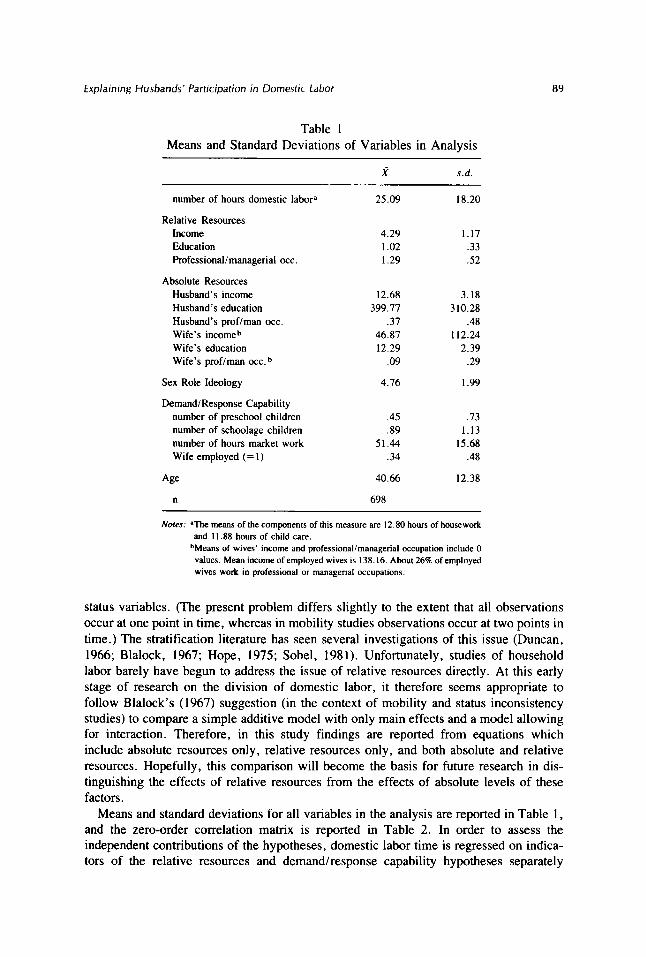
Table 1 Means and Standard Deviations of Variables in Analysis
x s.d.
number of hours domestic labora
Relative Resources Income Education Professional/managerial occ.
Absolute Resources Husband’s income Husband’s education Husband’s prof/man occ. Wife’s incomeb Wife’s education Wife’s prof/man O C C . ~
Sex Role Ideology
Demand/Response Capability number of preschool children number of schoolage children number of hours market work Wife employed (= 1)
Age
n
25.09
4.29 1.02 1.29
12.68 399.11
.31 46.87 12.29
.09
4.16
.45
.89 51.44
.34
40.66
698
18.20
1.17 .33 .52
3.18 310.28
.48 112.24
2.39 .29
I .99
.13 1.13
15.68 .48
12.38
Nofes: aThe means of the components of this measure are 12.80 hours of housework and 11.88 hours of child care.
bMeans of wives’ income and professional/managenal occupation include 0 values. Mean income of employed wives is 138.16. About 26% of employed wives work in professional or managerial occupations.
status variables. (The present problem differs slightly to the extent that all observations occur at one point in time, whereas in mobility studies observations occur at two points in time.) The stratification literature has seen several investigations of this issue (Duncan, 1966; Blalock, 1967; Hope, 1975; Sobel, 1981). Unfortunately, studies of household labor barely have begun to address the issue of relative resources directly. At this early stage of research on the division of domestic labor, it therefore seems appropriate to follow Blalock’s (1967) suggestion (in the context of mobility and status inconsistency studies) to compare a simple additive model with only main effects and a model allowing for interaction. Therefore, in this study findings are reported from equations which include absolute resources only, relative resources only, and both absolute and relative resources. Hopefully, this comparison will become the basis for future research in dis- tinguishing the effects of relative resources from the effects of absolute levels of these factors.
Means and standard deviations for all variables in the analysis are reported in Table 1, and the zero-order correlation matrix is reported in Table 2. In order to assess the independent contributions of the hypotheses, domestic labor time is regressed on indica- tors of the relative resources and demand/response capability hypotheses separately
Tabl
e 2
Zero
-Ord
er C
orre
latio
n M
atrix
I 2
3 4
5 6
7 8
9 10
II
I2
13
14
I5
1.
2.
3.
4.
5.
ID
6.
7.
8.
9.
10.
11.
12.
13.
14.
15.
16.
0
Rela
tive
inco
me
Educ
atio
n ra
tio
Rela
tive
prof
lman
Ed
ucat
ion
Inco
me
Prof
essi
onal
lman
ager
ial
occ.
Se
x ro
le i
deol
ogy
num
ber
of p
resc
hool
sch
ildre
n nu
mbe
r of
scho
olag
e ch
ildre
n nu
mbe
r of
hour
s m
arke
t wor
k W
ife e
mpl
oyed
A
ge
Dom
estic
lab
or ti
me
Wife
’s i
ncom
e W
ife’s
edu
catio
n W
ife’s
pro
flman
- .0
2 .2
3 -.
I6
-.05
-.63
.I
5 -.
05
-.01
-.
I6
-.29
-.
07
.I6
-.I1
.05
.0
3 .I
4 .0
5 -.
86
.05
.07
.15
-.02
-.
11
-.I2
.0
2 -.
I3
.07
-.44
.01
.30
.I7
.84
- .0
2 - .0
2 .04
.08
-.21 .09
- .0
7 -.
I4
.I1
- .3
9
.I8
.45
.30
.I0 .oo
- .0
3 .0
1 -.2
0 .06
.07
.61
.30
.I9
.07
- .0
9 .I
0 .I
1
- .0
4 .I
0 - .0
9 .0
1 .I
5 .0
1
.I5
.01
.01
-.07
.0
4 -.
06
.03
.05
.01
.28
-.I7
-.0
3 -.
I0
.09
-.I7
-.4
6 -.
03
-.08
-.
01
-.07
-.06
-.09
-.05
.33
.26
-.21
.0
2 -.2
8 .0
5 .2
2 -.
12
-.05
-.08
.5
8 -.
05
-.02
.33
.32
.04
-.02
-.01
.I
3 -.
I4
-.03
.I3
.I8
.29
-.08
-.05
-.08
.42
-.01
-.03
.34
.37
Explaining Husbands’ Participation in Domestic Labor 91
Table 3 Determinants of Husbands’ Domestic Labor Time (n= 698)
(Table 3). The effects of sex role ideology (and age) on domestic labor time are reported in Table 2. Table 4 reports the net effects of all the predictor variables on domestic labor time.
Table 2 indicates that sex role ideology is not significantly correlated with domestic labor time (r = - .05). The resource hypothesis does not fare much better in Table 3. Whether absolute, relative, or both absolute and relative indicators are estimated, resource variables alone explain no more than 2.4 percent of the variation in domestic labor time. This analysis suggests that absolute professional or managerial employment and income decrease domestic labor time which is consistent with the relative resources hypothesis. However, the negative effect of the education ratio in Equation (lb) implies that the higher a wife’s education is relative to her husband, the less domestic labor he performs which is counter to the resources hypothesis. Also, the positive effect of education in Equation (la) supports the ideology rather than the resources hypothesis. Relative income exerts no effect. Thus this analysis provides very weak support for the relative resources hypothesis.
Indicators of the demandhesponse capability hypothesis explain almost 25 percent of the variation in husbands’ domestic labor time. This is very close to the amount of variation explained when indicators of all three hypotheses are included in the equation simultaneously (see Table 4). All four measures of demandhesponse capability signifi- cantly affect men’s domestic hours in the direction predicted, although the effect of wife’s employment status is small.
92 THE SOCIOLOGICAL QUARTERLY Vol. 26/No. 1 11985
Table 4 Determinants of Husbands' Domestic Labor Time (n=698)
Findings from the simultaneous estimation of all the independent variables are con- sistent with the results in Table 3. Findings from the equations reported in Table 4 are quite similar. These results provide the strongest support for the demandlresponse ca- pability hypothesis. Indicators of this perspective (except absolute earnings, discussed below) significantly influence husbands' domestic labor time. In fact, number of pre- school children, number of school-age children and number of hours in market work are the strongest predictors of time spent in domestic labor relative to all other variables in each equation. As expected, number of children increases domestic labor time, and number of market work hours decreases domestic hours.4
The effect of another indicator of demand/response capability, spouse's employment status, is significant but of lesser magnitude than the effect of the other three variables in the analysis. This variable is highly colinear with relative income. The estimate of wife's employment status in Equation (2) of Table 3 avoids any bias that might be generated from this collinearity and, therefore, probably is the more reliable estimate. This metric coefficient indicates that men whose wives are employed spend about three hours more each week in housework and child care than do men whose wives are not employed. This breaks down roughly to 26 minutes a day, most of which probably is spent in child care as
Explaining Husbands’ Participation in Domestic Labor 93
opposed to housework (Pleck and Lang, 1978). When the equation is estimated with an interval-level measure of wives’ hours in market work substituted for the categorical variable, the estimate of the interval variable indicates that for each hour per week wives spend in paid work, husbands’ domestic time increases by about five minutes per week (not shown tabularly).
Generally, most studies in this area found no influence of wives’ employment status on husbands’ domestic participation (Vanek, 1974; Walker and Woods, 1976; Szinovacz, 1977; Geerken and Gove, 1983). The present analysis, however, is consistent with a few others analyses which have found a slight increase in men’s domestic labor time when their wives work outside the home for pay (Weingarten, 1978; Pleck, 1979; Huber and Spitze, 1983). According to Pleck, the latter pattern reflects the beginnings of change in the male role, although Huber and Spitze are less optimistic regarding future change in the division of domestic labor.
The estimate for age indicates that younger men do significantly more housework and child care than do older men. This effect does not seem to reflect ideological concerns since there is no indication that adherence to egalitarian sex role attitudes increases men’s participation in household labor. Surprisingly, a nontraditional sex role ideology de- creases men’s domestic labor time. Although the magnitude of this coefficient is small, it does attain statistical significance. This finding counters previous research (Stafford et al., 1977; Huber and Spitze, 1983) which finds that men who adhere to nontraditional ide- ology perform more household labor. Another indicator of ideology, absolute level of education, increases domestic hours in Equation (1) but exerts no effect in Equation (3). Thus, the ideology hypothesis, as presently conceptualized, receives little confirmation from this analysis.
The relative resources hypothesis does not receive strong support from this analysis either. Neither absolute nor relative measures of income contribute anything to the estima- tion of domestic work hours in Table 4. The income effect can be investigated further. First, it is possible that the aforementioned collinearity between relative income and spouse’s employment status might confound the effect of relative income. Therefore, Equation (2a) is estimated with spouse’s employment status omitted [Equation (2b)l. However, the estimate for relative income in Equation (2b) still is insignificant. Second, the gross effect of relative income in Equations (lb) and (lc) in Table 3 also is negligible. Third, when the model is estimated for men with employed wives, another relative income measure, wife/husband income ratio, does not influence domestic hours (not shown tabularly). Lastly, because Geerken and Gove found evidence of a curvilinear relationship between earnings and domestic hours, Equation (1) was reestimated with two dummy variables reflecting husband’s high and low income, with the middle-income level designated as the reference ~a tegory .~ Neither categorical variable exerted a significant effect on domestic hours. Relatedly, when the equation was estimated with logged in- come, no effect was observed. Hence, there is no evidence of a linear or curvilinear relationship between absolute or relative income and men’s domestic participation. (Be- cause earnings is also an indicator of husbands’ capacity to respond to domestic work demands-in terms of purchase of labor-saving devices and paid domestic assistance- this aspect of the demandhesponse capability hypothesis also finds no support.)
The wifelhusband education ratio in Table 4 exerts a negative effect which indicates that the closer couples are in education resources (which presumably would bestow more power on the wife), the less time husbands spend in domestic labor. Thus, consistent with
94 THE SOCIOLOGICAL QUARTERLY Vol. 26/No. 1 /1985
Huber and Spitze’s (1983) conclusions, education does not appear to function as a re- source here. Education may reflect ideological concerns though, since the coefficient for absolute education in Equation (1 ) [but not in Equation (3)] indicates that the more education husbands have, the more domestic work they perform. Finally, men’s domestic labor time is not affected by either absolute or relative measures of employment in professional or managerial occupations. Clearly, these results do not support the relative resources hypothesis.
These findings concerning resources are important, for it is often assumed that profes- sional and middle-class persons are in the forefront of gender role change. This assump- tion underlies the expectation that higher-class men will be participating more in house- work and child care. Importantly, there is little empirical support for this contention. Instead, this analysis suggests that what best explains variation in domestic labor time are indicators of the demands on husbands to perform housework and child care and their capacity to respond to these demands. Thus, number of children, number of hours spent in paid work, and, less importantly, spouse’s employment status are the strongest predictors of husbands’ time spent in domestic labor.
CONCLUSIONS This study has evaluated three hypotheses concerning men’s participation in domestic activities. The relative resources hypothesis suggests that absolute and relative measures of resources, such as education, occupational position, and earnings, will decrease men’s household labor time either because of the power that accrues to individuals with these resources or because such socioeconomic characteristics increase the value of market work more than the value of domestic work. The ideology hypothesis posits that ad- herence to traditional sex role ideology decreases men’s domestic hours. Lastly, the demand/response capability hypothesis states that indicators of the demands on husbands to perform household tasks, such as number of children and spouse’s employment status, along with their capability to fulfill those demands, as indicated by the time spent in paid work, determine the time men devote to housework and children.
Findings from this analysis overwhelmingly support the demand/response capability hypothesis as the best explanation of domestic labor time. Number of children, number of hours spent in market work, and spouse’s employment status are, along with age, the strongest predictors of husbands’ domestic labor time. Contrary to the ideology hypoth- esis, an egalitarian sex role ideology does not increase men’s domestic hours. In fact, it slightly decreases the domestic labor time of married men. Importantly, findings with both absolute and relative measures of husbands’ and wives’ resources do not support the relative resources hypothesis.
These results imply that neither attitude change nor socioeconomic status will alter the domestic division of labor. Rather, they suggest that younger men who have children, employed spouses, and jobs that do not require long work hours are most likely to be involved in housework and child care activities. These patterns are consistent with Beer’s (1983) conclusion that “a man’s class and class background are less important than the flexibility of time provided by his immediate occupational circumstances” (p. 43). Beer notes that the greater flexibility of time available to many professional men underlies the relationship often found between men’s professional status and their participation in housework. This contention is supported by the fact that the two studies that found that
€xplaining Husbands‘ Participation in Domestic Labor 95
professional men performed more domestic work than did nonprofessional men (Berk and Berk, 1978; Beer, 1983) did not include any measures of market work hours.
Many researchers have noted that gender role change in the home lags far behind changes that have already taken place in labor force participation and, to a lesser extent, in labor force achievements. This analysis suggests that wives’ expanded involvement in market work limits the available time they have for domestic pursuits. This in turn places demands on husbands, especially younger ones, to help relieve the strain by increasing their involvement in domestic activities. The extent to which these patterns portend genuine sex role change or simply reflect temporary, situation-specific behavior can not be determined with these cross-sectional data. However, findings from this study illumi- nate some key issues that should be explored in future investigations. First, does the negative age effect reflect a trend towards more egalitarian gender role socialization and behavior? Or does the age-domestic work relation suggest that younger men always have and probably will continue to perform more domestic labor? Second, will the trend towards increasing female labor force participation facilitate a long-term trend towards men’s greater domestic participation? Or will women cope with the double burden of paid and household work through strategies other than reliance on the domestic contributions of their spouses? Although researchers have been debating these issues, we still await analyses that can address them directly.
ACKNOWLEDGMENTS The author is indebted to Joseph F. Sheley for providing helpful comments. An earlier version of this paper was presented at the 1984 meeting of the American Sociological Association. San Antonio.
NOTES 1. Many respondents did not answer this question (EARN), but answered another income question where,
rather than state the dollar amount of their earnings, they had only to tell the interviewer the letter of the category that came closest to their annual income. Responses for this ordinal-level measure (INCBK) were categorized as follows: under $2000; $2000-5999; $6000-$9999; $loooO- 14999; $15000- 19999; 52ooOO-24999; $25000- 29999; $3oooO-34999; $35000 and over. The goal was to include those cases missing on EARN who had values on INCBK while also retaining the interval nature of the variable. In order to do this, a new variable was computed-income estimate (INCOMEST). If a respondent had answered the EARN question, his value for INCOMEST was his value for EARN. Then the means on EARN were calculated for each category of the ordinal measure. For those cases who were missing on EARN, but had identified a category on the ordinal variable, the mean of that category was assigned as their value for INCOMEST. It should be noted that this strategy assumes that the ordinal measure has a similar distribution as EARN. Those cases which were missing on both EARN and the ordinal variable were designated as missing on INCOMEST as well. Because the means of the two items are very similar, measurement error does not appear to be problematic here.
Note that the tasks mentioned in the question refer to both traditional masculine and feminine tasks and to tasks necessary for the functioning of the household conducted both inside and outside the home (see Pleck and Lang, 1978). Pleck and Lang term this method of deriving estimates of domestic labor the “respondent summary estimate,” as opposed to the “time diary” approach, wherein respondents record all detailed activities they perform daily in the household (Walker and Woods, 1976; Berk and Berk, 1978). According to Pleck and Lang, the summary estimate yields values for housework that are about five hours higher per week than those derived from the diary approach. Pleck and Lang additionally note that respondents’ own summary estimates of the time they spend at paid work are also inflated in comparison to the time estimates derived from time diaries.
The analysis would benefit from a dependent variable that reflected the division of domestic labor; i.e., one that measured husbands’ domestic labor time compared to wives’ domestic labor time. The QES includes a
2.
3.
96 THE SOCIOLOGICAL QUARTERLY Vol. 26”. 1 /1985
question on spouse’s hours spent in child care but does not include an item on number of hours spouse spends in housework. Therefore, wives’ domestic labor time can not be measured with these data.
The flexibility of men’s employment situation has also been emphasized as a factor in their domestic participation (Beer, 1983). Unfortunately, no such measure is included in the data. A rough assessment of the relationship between flexibility and domestic hours was attempted by comparing the time spent in domestic labor by professional men whose occupations likely provide flexible work hours (n = 42) with the remaining professional men (n = 76). The first group included all types of teachers and writers, artists and entertainers. There was not a significant difference between these two groups in mean domestic hours. Thus, this exercise suggests that number of market hours is more important than the flexibility of market hours in influencing domestic participation.
All respondents whose weekly earnings were $275 or below were assigned a value of I on the low earnings dummy variable and all others, 0; respondents whose weekly earnings were $409 or above were assigned a value of 1 on the high earnings dummy variable and all others, 0. About one-third of the sample were in each of the high, medium, and low earnings categories.
4.
5 .
REFERENCES Becker, G. S.
1975 “A theory of marriage: part 11.’’ Journal of Political Economy 82 (March/April): 11-26. Beer, W. R.
1983 Househusbands: Men and Housework in American Families. New York: Praeger. Berch, B.
1983 The Endless Day: The Political Economy of Women and Work. New York: Harcourt Brace Jovano- vich.
“A simultaneous equation model for the division of household labor.” Sociological Methods and Research 6 (May): 431-465.
“Status inconsistency, social mobility, status integration and structural effects.” American So- ciological Review 32 (October): 790-801.
Blood, R. and D. Wolfe 1960 Husbands and Wives. New York: The Free Press.
Coverman, Shelley 1983 “Gender, domestic labor time, and wage inequality.” American Sociological Review 48 (October):
623-637.
“Methodological issues in the analysis of social mobility.” Pp. 90-95 in N. J. Smelser and S. M. Lipset ‘(eds.), Social Structure and Mobility in Economic Development. Chicago: Aldine.
“Education, wage rates, and the division of labor between husband and wife.” Journal of Marriage and the Family 39 (August): 473-483.
“Labor market participation of young married women: causes and effects.” Journal of Marriage and the Family 44 (May): 457-468.
“Everyone needs three hands: doing unpaid and paid work.” Pp. 249-273 in S. F. Berk (ed.), Women and Household Labor. Beverly Hills: Sage.
At Home and At Work: The Family’s Allocation of Labor. Beverly Hills: Sage.
“The family as the locus of gender, class and political struggle: the example of housework.” Signs 6 (Spring): 366-394.
“Models of status inconsistency and social mobility effects.” American Sociological Review 40 (June): 322-343.
Berk, R. and S. Berk 1978
Blalock, H. H., Jr. 1967
Duncan, 0. D. 1966
Farkas, G. 1976
Ferber, M. A. 1982
Glazer, N. 1980
Geerken, M. and W. R. Cove
Hartmann, H. I . 1983
1981
Hope, K. 1975
€xp/aining Husbands’ Participation in Domestic Labor 97
Huber, J. and G. Spitze
Paloma, M. and N. Garland 1983
1972
Sex Stratification: Children, Housework, and Jobs. New York: Academic Press.
“The married professional woman: a study in the tolerance of domestication.” Journal of Marriage and the Family 33 (November): 531-539.
“Determinants of male family-role performance.” Psychology of Women Quarterly 3 (Fall): 53-66.
“Men’s family work: three perspectives and some new data.” The Family Coordinator 28 (October):
Permcci, C. C., H. R. Pottes and D. C. Rhoads
Pleck, J. H. 1978
1979 481-488.
Pleck, J. H. and L. Lang 1978 “Men’s family role: it’s nature and consequence.” Working paper, Wellesley College Center for
Research on Women.
1979 Quality of Employment Survey, 1977: Cross-Section. Ann Arbor: Inter-University Consortium for Political and Social Research.
“Housework technology and household work.” Pp. 53-68 in Sarah F. Berk (ed.), Women and Household Labor. Beverly Hills: Sage.
Worlds of Pain. Life in the Working-class Family. New York: Basic Books.
“Sex role attitudes and social class: a reanalysis and clarification.” Journal of Comparative Family Studies 13 (Spring): 77-88.
“Diagonal mobility models: a substantively motivated class of designs for the analysis of mobility effects. ” American Sociological Review 46 (December): 893-906.
Stafford, R., E. Backman and P. Dibona “The division of labor among cohabiting and married couples.” Journal of Marriage and the Family 39 (February): 43-54.
“Role allocation, family structure and female employment.” Journal of Marriage and the Family 39 (November): 78 1-79 1.
“Causes and consequences of sex-role attitudes and attitude change.” American Sociological Review
Quinn, R. and G. Staines
Robinson, J. P. 1980
Rubin, L. B.
Smith, M. D. and L. J. Fisher 1976
1982
Sobel, M. 1981
1977
Szinovacz, M. E. 1977
Thornton, A, , D. F. Alwin and D. Camburn 1983
Vanek, J. 1974 “Time spent in housework.” Scientific American 231 (November): 116-120.
Walker, K. and M. Woods 1976 Time Use: A Measure of Household Production of Family Goods and Services. Washington, D.C.:
American Home Economics Association.
“The employment pattern of professional couples and their distribution of involvement in the fami- ly.” Psychology of Women Quarterly 3 (Fall): 43-52.