Explaining the Effect of Financial Development on the Quality of Property Rights Chandramouli Banerjee, Niloy Bose * and Chitralekha Rath † Preliminary Draft. Please do not cite. October 21, 2015 Abstract This paper offers an insight into understanding recent empirical findings which sug- gest that beyond a certain threshold, financial development can catalyze property rights reforms. The explanation is based on a simple trade-off between costs and benefits of securing property. Securing the right to property allows agents to post collateral against loans, bettering their terms. However, securing such rights is costly. We analyze this trade-off along the path of financial development to establish that financial development creates incentives for better property rights institutions. However, for such incentives to materialize, financial development must cross a threshold. JEL Classification : E02, E44. Keywords : Financial Development; Property Rights. * Corresponding Author: [email protected]† Banerjee, Bose and Rath: University of Wisconsin-Milwaukee, Department of Economics, 3210 North Maryland Avenue, Bolton Hall, Milwaukee 53211 USA
Transcript
Explaining the Effect of Financial Development on the Quality
of Property Rights
Chandramouli Banerjee, Niloy Bose∗ and Chitralekha Rath†
Preliminary Draft. Please do not cite.
October 21, 2015
Abstract
This paper offers an insight into understanding recent empirical findings which sug-
gest that beyond a certain threshold, financial development can catalyze property rights
reforms. The explanation is based on a simple trade-off between costs and benefits of
securing property. Securing the right to property allows agents to post collateral against
loans, bettering their terms. However, securing such rights is costly. We analyze this
trade-off along the path of financial development to establish that financial development
creates incentives for better property rights institutions. However, for such incentives
to materialize, financial development must cross a threshold.
JEL Classification: E02, E44.
Keywords: Financial Development; Property Rights.
∗Corresponding Author: [email protected]†Banerjee, Bose and Rath: University of Wisconsin-Milwaukee, Department of Economics, 3210 North
Maryland Avenue, Bolton Hall, Milwaukee 53211 USA
1 Introduction
There is a consensus that property rights encourage investment (Besley, 1995; Knack and
Keefer, 1995; Johnson et al., 2002), entrepreneurship (Murphy et al., 1991) and innovation
(Furman et al., 2002). Recently economists have also recognized that a system of strong
property rights can enhance efficiency in financial sectors. This is intuitive since legislation
protecting property often encompasses financial contracts (Porta et al., 2002; Claessens and
Laeven, 2003; Beck et al., 2005), and even when it does not, it can improve contracting
efficiency by allowing borrowers to pledge collateral (Djankov et al., 2007; De Soto, 2000;
Besley and Ghatak, 2009). Here the direction of causality runs from property rights to
financial development. But is it possible that the reverse is also true? There are reasons
to believe that this may be the case. For example, certain types of financial reforms, in
particular those that relax restrictions on the movement of capital can provide incentives for
managers and controlling shareholders to uphold contracts and to better protect minority
investors’ rights (Stulz, 2005). Alternatively, since engineering institutions that guard the
rights of investors is costly, deep financial markets can be a prerequisite for such institutions
to be viable (Miletkov and Wintoki, 2009). Using the Gwartney and Lawson index,1 Bose
et al. (2014) offer formal evidence in support of the view that increases in the size of the
financial sector catalyze property rights reforms and that such an effect is economically
meaningful.2 One of the goals of this paper is to offer an explanation for this empirical
regularity. We pivot our explanation on a set activities that form the basis of a financial
market and put forward a theoretical argument to suggest that a mature financial system
can in fact provide incentives to better codify and protect individuals’ right to ownership.
While there is mounting evidence to suggest that financial system can influence the
quality of property rights institutions, there is no reason to presume a linear relationship
between the two variables. In fact, a formal analysis of the data presented in the Section
2 strongly suggests a non-linear relationship. Even a cursory look at the data brings out
the non-linear pattern between the two variables. Suppose that we divide the time interval
1970-2005 into equal five year intervals and for each interval we calculate country specific
1This index published by Fraser Institute rates countries on a scale 0 to 10 - zero representing the lowest
quality of property rights institutions. Data is reported in five year intervals. See Gwartney et al. (2009)2For example, the mean property rights score in 2005 was 5.91 and the standard deviation was 1.85.
Depending on the methodology used, a one standard deviation increase in private credit from its average
value in 2005 (for a sample of nearly 100 countries) translates into a 0.5 to 1.0 point increase in the property
rights index.
1
average value of private credit to GDP ratio for a sample of 106 countries. Next, we
divide the sample into two-equal sized groups - one containing countries whose (average)
private credit-to-GDP ratio never exceeded 30 percent (low finance group) and the other
comprising of countries that have this ratio above 30 percent (high finance group). This
leaves us with a distribution of private credit-to-GDP ratio corresponding to each time
interval for each group of countries. Finally, we calculate the median of this distribution for
each time interval. This is the finance variable of our interest. In Figure 1 we plot an index
of property rights (Gwartney et al., 2009) over five year intervals from 1970 to 2005 against
the constructed finance variable for the preceding five year interval. In the low finance group
the private credit-GDP ratio and property rights do not appear to co-move. In the high
finance group, however, the changes in property rights closely track changes in the ratio of
private credit to GDP; suggesting that there may be differences in the way finance affects
property rights protection in different subsets of countries. We take cue from this cursory
evidence and undertake more formal tests with the data in Section 2. The analysis suggests
that there exists a threshold in the relationship between property rights and finance on the
basis of which we are able to isolate two distinct regimes; one in which the quality of the
financial system is poor and where its effect on property rights is weak, and one where the
practice of banking has evolved beyond a certain point such that further improvements in
access to credit are positively associated with the degree to which countries enforce property
rights.
In summary, the data points to two key stylized facts. The first fact is based on
conventional wisdom as well as on existing results (Bose et al., 2014) and points to a causal
relationship running from finance to the quality of property rights institutions. The second
pattern in the data that we present in this paper suggests a non-linear relationship between
the two variables. In this paper we seek to offer a theory of financial market that is able to
explain both patterns that are present in the data.
Our main argument revolves around a broad notion that the quality of institutions
is not impervious to the changes in prevailing economic and social conditions despite being
influenced by a cluster of exogenous initial conditions such as legal traditions or natural
endowments. In fact, institutions do change.3 Sometimes the proximate triggers for these
3In countries adopting market-oriented reforms, this change has been rapid. Based on an index published
by the Cato Institute, which ranks the quality of property rights institutions on a 10-point scale, property
rights strengthened in Chile from 1.1 in 1970 to 7.00 in 2006 - a rating comparable to that in Belgium and
0.7 points higher than that in Italy. Based on another indicator of institutional quality - an index assessing
constraints on the executive branch of government - Rodrik et al. (2004) report a 40 percent improvement
2
reforms have been shifts in ideology - Chile under Augusto Pinochet and China under Deng
Xiaoping are good examples. The triggers could also be related to economic conditions. For
example, the models of institutional change advocated by Demsetz (1967) and North (1981)
suggest that institutions evolve once the economic and/or social gains from institutional
change exceed the costs of not doing so. Both argue that technological innovation and
the development of new economic markets lead to the introduction of new institutional
arrangements or the reform of existing arrangements. Here, we build on these basic ideas
and argue that a changing economic environment induced by financial developments can
shape the evolution of property rights by altering tradeoffs between the costs and the benefits
of protecting property.
We offer a formal theoretical rationale using a simple model of financial intermedia-
tion with incomplete information. In our economy individuals must access external funds
to operationalize investments. Financial intermediaries ration credit because of the asym-
metric nature of information. As a result some borrowers are denied loans. Faced with
this possibility, borrowers post assets as collateral to improve the terms and conditions of
the loans they receive. However, the gaps in the legislative framework allow for encroach-
ment on these assets. This generates push back from property owners which can take many
forms. For instance, owners could litigate, they could employ private security, or they
could pay public authorities to protect their assets. Whichever is the preferred practice, it
comes at a cost that increases with the fraction of property that owners wish to safeguard.4
Protecting property offers additional non-trivial benefits via its effects on the contractual
arrangements with the lenders. Specifically, the more an individual spends securing prop-
erty, the more collateral an individual can post to better the terms and conditions of a
loan contract. Against this background, we show that the marginal net gain from posting
collateral increases with the level of financial development. As a result, mature financial
markets generate additional incentives for individuals to secure their right to ownership.
Individual initiative to protect property plays a pivotal role in our analysis. One
could however question the relevance of such initiative since laws that exist on the book
apply equally to all members of the society. Therefore, any private initiative is futile in
shaping the extent to which an individual is able to protect his/her own property. We,
between the 1970s and 1990s in 20 of the 71 countries that composed their sample.4We do recognize that costs of enforcing property right could also take a more subtle form such as
a misallocation of talent from productive to unproductive sectors (Acemoglu and Verdier, 1996), and an
increase in market concentration (Furukawa, 2007). To keep the argument streamlined and tractable, we
leave these costs out of our analysis.
3
however, argue otherwise and view effective property rights as a culmination of the laws
that exist on books and the initiatives that are taken by the members of society at an
individual or as a group. For example, there may exist a law that make encroachment upon
privately held land illegal. Yet, an individual must undertake a variety of costly procedures
such as surveying the land, drawing up a legal deed, notarizing the deed in court, etc. to
uphold such a law. An individual’s effective right to the property also depends on the
legal costs which he/she is willing to incur in an event of encroachment. Similarly, putting
a fence up around the property or taking measures to prevent trespassing is a common
private initiative among land owners. Costly initiatives such as these pre-emptively protect
against encroachment and uphold law that exist on books. Also, it is also often the case that
individuals as group rally their cause and shape the law that exist on books by undertaking
costly initiatives (e.g. hiring lobbyists and public relation experts).5 These observations
let us take the stand that private initiatives do shape the effectiveness and the quality of
property rights institutions and whatever the de jure condition of property right protection
may be, it is the de facto outcome that we are interested in this paper. Finally, it is also
worth noting that indices that are commonly used to measure the quality of property rights
protection (including the Gwartney and Lawson property rights index) are drawn not only
on the basis of the laws that exists on books but also on factors that reflect private initiatives
undertaken to uphold such laws.6
In the analysis that follows, we exploit the tradeoff between the costs and benefit
of protecting property from the perspective of an individual to draw conclusions at the
aggregate level. In doing so, we do not simply aggregate individuals’ behaviors. Instead we
recognize that an individual’s cost of protecting property is also affected by the decisions
that other individuals make with regard to protecting their own property. This opens the
analysis up to a richer set of possibilities and the equilibrium that prevails is uniquely
determined by the level of financial development. In particular, beyond a threshold level
5For example, the Motion Pictures Association of America (MPAA) which represents the interests of six
major Hollywood studios has long advocated for the motion picture and television industry through lobbying
to protect creative content from piracy and curb copyright infringement. Some of the anti-piracy measures
used by them include lobbying for legislature, hosting publicity campaigns against piracy and widespread
legal action against entities that engage in such activities.6For example, one of the bases of the Gwartney and Lawson Property Rights Index is the variable Integrity
of the Legal System, sourced from the International Country Risk Guide’s Political Risk Component I for
Law and Order. This variable is constructed to assess the “strength and impartiality of the legal system”
(law on the books) as well as “popular observance of the law” which depends on initiatives to uphold such
law (law in practice). Both these measures receive equal weight in the construction of the variable.
4
of financial development, the number of agents initiating safeguards against encroachment
increases monotonically with the development of the banking system. Below this threshold,
the state of financial development has no effect on the degree to which society secures private
property.
The remainder of the paper is organized as follows. Section 2 offers formal evidence
in support of non-linearity in the relationship between property rights and finance. Section
3 describes the economic environment. In Section 4, we describe and solve the financial
contract between financial intermediaries and borrowers in an imperfect information setting.
Section 5 analyzes the effect of financial development on the incentive to protect property
at both individual and aggregate levels. Section 6 concludes with some comments.
2 A Closer Look at the Data
Though finance matters for the development of property rights institution, there is no reason
to presume linearity in their relationship. In this section, we look deeper into the data and
use two separate methods to examine potential non-linearity in the relationship. As a
first pass, we estimate a semiparametric partially linear regression model where the finance
variable enters the regression additively, but we do not impose any a-priori restriction on
the relationship between finance and property rights. Accordingly, our regression equation
takes the following form:
yi = x′iβ + g(zi) + ei (1)
where the variables yi and zi represent the average measure of property rights (drawn from
Gwartney et al. (2009)) and the average private sector credit to GDP ratio7 for country i,
respectively. According to the existing literature, institutions are influenced by a cluster of
exogenous initial conditions, such as legal origins (La Porta et al., 1999), settler mortality
rates (Acemoglu et al., 2001, 2002), and ethnic compositions (Easterly and Levine, 1997).
Accordingly, the vector xi consists of a dummy for British legal origin, a country’s latitude
(which is a proxy for settler mortality), a measure of ethnic fractionalization, and a dummy
variable that takes the value of 1 if the country has experienced a crisis in the preceeding
seven or less years. This serves as our baseline specification. With the exception of a
financial crisis variable and a dummy for Catholicism, the above specification is identical
to the one considered by Ayyagari et al. (2008).
7To be precise, our finance variable is the time average of log(1 + private credit to GDP)
5
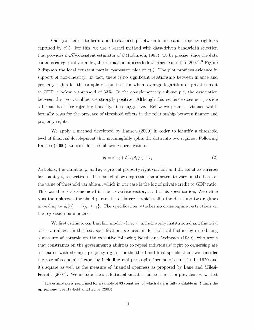
Our goal here is to learn about relationship between finance and property rights as
captured by g(·). For this, we use a kernel method with data-driven bandwidth selection
that provides a√n-consistent estimator of β (Robinson, 1988). To be precise, since the data
contains categorical variables, the estimation process follows Racine and Liu (2007).8 Figure
2 displays the local constant partial regression plot of g(·). The plot provides evidence in
support of non-linearity. In fact, there is no significant relationship between finance and
property rights for the sample of countries for whom average logarithm of private credit
to GDP is below a threshold of 33%. In the complementary sub-sample, the association
between the two variables are strongly positive. Although this evidence does not provide
a formal basis for rejecting linearity, it is suggestive. Below we present evidence which
formally tests for the presence of threshold effects in the relationship between finance and
property rights.
We apply a method developed by Hansen (2000) in order to identify a threshold
level of financial development that meaningfully splits the data into two regimes. Following
Hansen (2000), we consider the following specification:
yi = θ′xi + δ′nxidi(γ) + ei (2)
As before, the variables yi and xi represent property right variable and the set of co-variates
for country i, respectively. The model allows regression parameters to vary on the basis of
the value of threshold variable qi, which in our case is the log of private credit to GDP ratio.
This variable is also included in the co-variate vector, xi. In this specification, We define
γ as the unknown threshold parameter of interest which splits the data into two regimes
according to di(γ) = 1qi ≤ γ. The specification attaches no cross-regime restrictions on
the regression parameters.
We first estimate our baseline model where xi includes only institutional and financial
crisis variables. In the next specification, we account for political factors by introducing
a measure of controls on the executive following North and Weingast (1989), who argue
that constraints on the government’s abilities to repeal individuals’ right to ownership are
associated with stronger property rights. In the third and final specification, we consider
the role of economic factors by including real per capita income of countries in 1970 and
it’s square as well as the measure of financial openness as proposed by Lane and Milesi-
Ferretti (2007). We include these additional variables since there is a prevalent view that
8The estimation is performed for a sample of 83 countries for which data is fully available in R using the
np package. See Hayfield and Racine (2008).
6
real per-capita incomes and greater openness are associated with stronger property rights
(Gradstein, 2004; Wei, 2000).9
The results are reported in Table 1. The presence of a threshold is evident in all three
specifications. In the first two specifications, the regimes split at γ = 3.39. Since our finance
variable is defined as log[1+(private credit)/GDP], the obtained value γ is equivalent to a
private credit to GDP ratio of 28.67% ( = exp(3.39)-1). Whereas, in the third specification,
the split occurs at the private credit to GDP ratio of 28.37% ( = exp(3.3857)-1). These
threshold values are consistent with the turning point that we obatined in our earlier semi-
parametric exercise. Significantly, all three specifications convey the same message: The
finance variable is strongly and significantly associated with property rights only in the
higher financial regimes. In other words, a meaningful relationship between the two variables
transpires only the level of financial development surpasses a threshold level. In the next
section, we develop a unified theoretical framework that not only draws line from financial
development to property rights also explains why a certain level of financial maturity is
needed before financial development can shape incentives to protect property.
3 The Environment
In our model, events unfold in a small open economy over two periods. The economy is
populated with a countably infinite number of agents of unit mass. We suppose that these
agents are risk neutral, deriving linear utility from consumption which takes place at the
end of the second period. Each agent is endowed with an unit of an asset.10 If rights to
property on this asset is fully enforced, then an agent can sell this asset at the end of the
second period for a given market value υ. An agent also has an opportunity to partake in
a business venture (or project) during the first period of her life. A venture undertaken at
time t requires a fixed investment11 of x. The project generates certain amount of output
at time t + 1, each unit of which is sold at a formal market for a price ρt+1. We assume
that the demand for the product is given and is downward sloping so that the market price
ρt+1 is inversely related to the quantity of product that is available in the market at t+ 1.
9The estimation is carried out with the same sample of 83 countries as in the previous exercise in R using
a code made available by Bruce E. Hansen on his personal webpage. The relevant program can be found
here: http://www.ssc.wisc.edu/∼bhansen/progs/ecnmt 00.html.10For the purpose of exposition, it is beneficial to think of this asset as a plot of uncultivated land.11Again, one can contextualize x as the cost of investment (purchase of machinery, fertilizer etc.) that is
necessary for making the land fit for cultivation.
7
Since earnings generated from assets are realized at the end of the second period, agents are
unable to finance their own projects. Instead they must contract with banks to obtain a loan
of quantity x. We assume that these banks operate in a competitive environment and have
access to a perfectly elastic supply of loanable funds which are priced at the exogenously
determined world interest rate, r.
While the cost of operationalizing the asset is same for all individuals, we assume
that these project themselves can be of two types - low risk (type-L) or high risk (type-
H). A type-L project turns x units of the consumption good into Qx units of output with
probability pL = 1, whereas a type-H project converts the same investment x into Qx units
of output with a probability pH ∈ (0, 1), and 0 otherwise. We assume the each agent faces
an ex-ante probability λ ∈ (0, 1) of owning a type-L project, and this realization is private
information.12 As it will become apparent, some loan applicants may be adversely selected
and denied credit since the project type associated with any given loan applicant is private
information. If an applicant doesn’t receive a loan, she scales down the size of her business
and produces a small amount of output for her own consumption. This outside opportunity
generates αH and αL units of the consumption to the owners of type-H and type-L projects
respectively, and we assume αL > αH . For notational convenience we normalize αH = 0.13
In our economy, the arrangements that ensure full rights to property are absent to
some degree. However, the quality of property rights institution, whether formal or informal,
are not exogenously given. Instead they evolve, driven by the strength of private incentives
to invest in property right protection. Though property rights are slack, we assume that
an owner of an asset can protect a fraction γ, of the value of her initial endowment by
incurring a monetary and/or time cost in the amount of the τγ. In practice, this cost can
take various forms, such as legal costs, the costs of hiring private security, or contribution
to lobbying costs incurred when establishing new case law that strengthens property rights
(Lanjouw et al., 1998; Lanjouw and Schankerman, 2001) etc.
The timing of events in our economy proceeds as follows. Prior to gaining access
12Alternatively we could assume agents are randomly endowed with different abilities. For example, a
fraction λ of agents could be endowed with better skills such that the expected returns to their investments
are higher. We simplify matters by assuming that projects with different risk characteristics are randomly
allocated across individuals.13Strictly, it is only necessary to assume that outside opportunities across the two type of borrowers differs.
There are various ways to motivate this. For example, it is possible to interpret this difference as a result of
skill heterogeneity: individuals with higher skills can not only generate higher expected project output, but
the value of their outside opportunity is also greater.
8
to a project, agents choose a value of γ, i.e. they decide how much property they want to
safeguard from predation. Next agents are randomly and privately assigned a project, such
that a fraction λ are assigned to type-L projects and the remaining (1 − λ) are assigned
type-H projects. Once projects are assigned, agents seek to operationalize these ventures,
by applying for loans from financial intermediaries. The agents post a fraction of the asset
in possession (net of predation) as collateral. Hence, the terms and conditions for loans are
influenced an agent’s choice of γ. In the second period, projects generate incomes with which
agents pay off loans and also consume. The outcomes that transpire from these decisions
are determined by solving backwards through the sequence of events. In particular, we first
determine how the loan contract is influenced by the choice of γ. This information is then
used in following sections to pin down the optimal value of γ for an individual and for the
economy as a whole.
4 Financial Contracts
In the first period, borrowers approach banks for loans to finance investments. The id-
iosyncratic credit risk associated with each borrower is private information. However, the
aggregate ex-ante distribution of project types, the project technology, and the outside op-
portunities faced by type-L versus type-H investors are common knowledge. In addition,
loan applicants also reveal the value of their assets (net of predation), γυ, which is costlessly
verifiable by financial intermediaries.
We suppose that banks incur a cost when contracting loan agreements. We denote
this cost by δ > 0. In practice, costs of financial intermediaries include the cost of provid-
ing liquidity services, agency costs, such as those associated with processing information,
enforcing contracts, and screening. We assume that these costs decline along the path of
financial development. There is certainly an empirical basis for this assumption. Two em-
pirical measures of intermediation costs are banks’ overhead expenditure as a proportion of
total assets and banks’ net interest rate margin. It is well documented that both measures
tend to be higher in less developed financial sectors (Demirguc-Kunt and Huizinga, 2000;
Demirguc-Kunt et al., 2003). Accordingly, we interpret lower values of δ to reflect a more
developed financial system and we assume that the value of δ is known to the financial
intermediaries.
Given the above information, a lender offers contracts to borrowers, the acceptance
of which implies a binding agreement committing the former to a transfer of funds in the
9
amount x to a borrower and the latter to a repayment from her future project income.
We assume that financial intermediaries operate in a competitive environment and that
the terms and conditions of loan contracts offered in the market is common knowledge.
Accordingly, loan-applicants will only approach financial intermediaries if the contracts
offered are not dominated by other contracts available in the market. Thus, in equilibrium,
banks earn zero normal profits.
Recall that the project type associated with any given loan application is private
information. In response, financial intermediaries exploit known differences between the
type-L and type-H project owners when designing a menu of contracts that induces self-
selection. In particular a contract offered by the bank is a pair Ci ≡ Ri, πi for i ∈ H,L,where Ri is the gross lending rate for a contract of type-i and πi ∈ [0, 1] is the the probability
that a type-i applicant is granted a loan. For a contract that is granted at time t, the type-i
borrower receives utility Ui ≡ πi[pi(Qρt+1−Ri)x+γυ] + (1−πi)[αi+γυ] where i ∈ H,L,with pH < pL = 1 and αL > αH = 0. The first term in this expression is the net payoff to a
borrower from risky project in the event a loan is granted and the project is successful. The
second term is the payoff in the event that the project is not funded. It is easy to see that
since αL > αH , the indifference curves of the two types of borrowers satisfy single-crossing
property in the contract plane. This enables lenders to separate borrowers according to
their risk types by offering a menu of contracts that are individually rational and incentive
compatible.14 The following proposition fully describes the elements of the contract.
Proposition 1 Let r denote the cost of funds for financial intermediaries. If (Qρt+1 −RL)x > αL, then the time t equilibrium contract given γ, r, δ is characterized by:
RL =xr + δ
x; RH =
xr + δ − (1− pH)γυ
pHx(3)
πL =pHQρt+1x− xr − δ + (1− pH)γυ
pH(Qρt+1x− xr − δ), πH = 1 (4)
Proof The banks’ zero profit condition on a contract Ri, πi is given by:
piRix+ (1− pi)γυ = rx+ δ (5)
The expression of the left in (5) is the banks’ expected earnings from a loan; it is the sum
of the banks’ interest earnings in case of no default (when the project is successful) and
14For similar arguments, see Rothschild and Stiglitz (1976), Bencivenga and Smith (1993), and Bose and
Cothren (1996).
10
the amount that the bank can recover by appropriating the collateral posted in case of a
default (when the project is unsuccessful). The expression on the right shows the cost of
lending, the sum of the cost of acquiring funds and the cost of intermediation.
The expressions for Ri for i ∈ H,L follows immediately from the banks’ zero
profit condition (5) where we assume pL = 1. We also assume γυ < rx+ δ, i.e. there is risk
associated with lending. This implies, from (3) and (4) that RL < RH .
Note that the type-H individuals earn lifetime utility UH = πH [pH(Qρt+1−RH)x+γυ
from their contracts CH and type-L individuals earn UL = πL[pL(Qρt+1 − RL)x] + (1 −πL)αL+γυ from CL. Now consider the a full information scenario, where banks are able to
distinguish between type-L and type-H individuals. In such a scenario, the offered contracts
will still earn zero profit for the lenders under competition and banks have no need to
deny credit to individuals. Let us define these first best contracts CFi ≡ Ri, πi = 1 for
i ∈ H,L. Since RL < RH , the following inequalities hold: UH(CFH) < UH(CFL ) and
UL(CFH) < UL(CFL ). It is clear that if first best contracts are being offered, then a type-H
individual has an incentive to misrepresent herself as being type-L (pooling on CFL ) but
the converse isn’t true. Hence, in order to separate the two types through self-selection,
the banks distort the contracts for type-L individuals CFL but have no need to change
the contracts for type-H individuals who get their first best contracts CFH = RH , πH =
1. Given the expressions for RL and RH , the contract for the type-L borrower is then