Explicit Magnus expansions for nonlinear equations Fernando Casas a and Arieh Iserles b § a Departament de Matem`atiques, Universitat Jaume I, 12071-Castell´on, Spain b Department of Applied Mathematics and Theoretical Physics, University of Cambridge, Wilberforce Rd., Cambridge CB3 0WA, United Kingdom E-mail: [email protected], [email protected]Abstract. In this paper we develop and analyse new explicit Magnus expansions for the nonlinear equation Y 0 = A(t, Y )Y defined in a matrix Lie group. In particular, integration methods up to order four are presented in terms of integrals which can be either evaluated exactly or replaced by conveniently adapted quadrature rules. The structure of the algorithm allows to change the step size and even the order during the integration process, thus improving its efficiency. Several examples are considered, including isospectral flows and highly-oscillatory nonlinear differential equations. AMS classification scheme numbers: 65L05, 41A55, 22E60 § To whom correspondence should be addressed
Transcript
Explicit Magnus expansions for nonlinear equations
Fernando Casasa and Arieh Iserlesb§a Departament de Matematiques, Universitat Jaume I, 12071-Castellon, Spainb Department of Applied Mathematics and Theoretical Physics, University ofCambridge, Wilberforce Rd., Cambridge CB3 0WA, United Kingdom
Abstract. In this paper we develop and analyse new explicit Magnus expansions forthe nonlinear equation Y ′ = A(t, Y )Y defined in a matrix Lie group. In particular,integration methods up to order four are presented in terms of integrals which can beeither evaluated exactly or replaced by conveniently adapted quadrature rules. Thestructure of the algorithm allows to change the step size and even the order duringthe integration process, thus improving its efficiency. Several examples are considered,including isospectral flows and highly-oscillatory nonlinear differential equations.
Explicit Magnus expansions for nonlinear equations 2
1. Introduction
Nowadays the so-called Magnus expansion constitutes a widespread tool to construct
approximate solutions of non-autonomous systems of linear ordinary differential
equations. As is well known, the basic idea is to represent the solution of
Y ′ = A(t)Y, Y (0) = Y0, (1)
where A is a n × n matrix, in the form Y = exp(Ω(t))Y0 and express Ω as an infinite
series Ω(t) =∑∞
k=1 Ωk(t), whose terms are linear combinations of integrals and nested
commutators involving the matrix A at different times [21]. In particular, the first terms
read explicitly
Ω1(t) =
∫ t
0
A(t1)dt1, Ω2(t) =1
2
∫ t
0
dt1
∫ t1
0
dt2[A1, A2],
where Ai ≡ A(ti) and [X, Y ] ≡ XY − Y X is the commutator of X and Y . Explicit
formulae for Ωk of all orders have been given in [18] by using graph theory, whereas in [20]
a recursive procedure for the generation of Ωk was proposed. Different approximations
to the solution of (1) are obtained when the series of Ω is truncated. This procedure has
the very attractive property of ensuring preservation of important qualitative properties
of the exact solution at any order of truncation.
Since the 1960s, the Magnus expansion has been successfully applied as an analytic
tool in numerous areas of Physics and Chemistry, from nuclear, atomic and molecular
Physics to NMR and Quantum Electrodynamics (see [1] for a list of references). Also a
convergence proof for the series defining Ω has been obtained [1].
In recent years, Iserles and Nørsett [18] used rooted trees to analyse the expansion
terms, leading to a recursive procedure to generate Ω and constructing practical
algorithms for the numerical integration of equation (1). The resulting schemes are
prototypical examples of geometric integrators : numerical methods for discretising
differential equations which preserve their known qualitative features, such as invariant
quantities and geometric structure [13]. By sharing such properties with the exact
solution, these methods provide numerical approximations which are more accurate and
more stable for important classes of differential equations, such as those evolving on Lie
groups. In addition, several integrators based on the Magnus expansion have proved to
be highly competitive with other, more conventional numerical schemes with respect to
accuracy and computational effort [2, 3].
In this respect, there are two important factors involved in the process of rendering
Magnus expansion as a class of numerical integrators. On the one hand, the structure of
the Magnus series is such that the number of matrix evaluations required to compute all
the multivariate integrals in the expansion to a given order is the same as the cost of the
single quadrature formula for Ω1 [18]. On the other hand, an optimization procedure
can be designed to reduce a great deal the number of commutators required by the
scheme [3].
It is perhaps for these reasons that, although these algorithms have been primarily
designed for linear problems, where the matrix function A depends on time only, several
Explicit Magnus expansions for nonlinear equations 3
attempts have been made to generalise the formalism when A = A(t, Y ). In that case,
though, multivariate integrals depend also on the value of the (unknown) variable Y at
quadrature points. This leads to implicit methods and nonlinear algebraic equations
in every step of the integration [27] which in general cannot compete in efficiency
with other classes of geometric integrators such as splitting and composition methods.
An interesting alternative have been proposed by Blanes and Moan [4]: they use a
conveniently modified version of the Magnus expansion to construct a new class of
splitting methods for non-autonomous Hamiltonian dynamical systems.
In this paper we try to overcome some of the aforementioned difficulties and develop
new explicit Magnus expansions for the nonlinear equation
Y ′ = A(t, Y )Y, Y (0) = Y0 ∈ G, (2)
where G is a matrix Lie group, A : R+ × G −→ g and g denotes the corresponding
Lie algebra (the tangent space at the identity of G). Equation (2) appears in relevant
physical fields such as rigid mechanics and in the calculation of Lyapunov exponents
(G ≡ SO(n)), Hamiltonian dynamics (G ≡ Sp(n)) and Quantum Mechanics (G ≡SU(n)). In fact, it can be shown that every differential equation evolving on a matrix
Lie group G can be written in the form (2). Moreover, the analysis of generic differential
equations defined in homogeneous spaces can be reduced to the Lie-group equation (2)
[26]. It is therefore of the greatest interest to design numerical geometric integration
schemes for the system which are computationally as efficient as possible.
One common technique to solve eq. (2) whilst preserving its Lie group structure is
to lift Y (t) from G to the underlying Lie algebra g (usually with the exponential map),
then formulate and solve there an associated differential equation and finally map the
solution back to G. In this way the discretization procedure works in a linear space
rather than in the Lie group. In particular, the idea of Munthe-Kaas is to approximate
the solution of the associated differential equation in the Lie algebra g by means of
a classical Runge–Kutta method, thus obtaining the so-called Runge–Kutta–Munthe-
Kaas (RKMK) class of schemes [24, 17].
Here new Lie group solvers up to order four for (2) are presented. The new schemes
are explicit by design and are expressed in terms of integrals which can be replaced by
different quadrature rules. It is also possible to change the step size and even the order
at each integration step, so that although their computational effort per step exceeds
some other algorithms, with an optimal implementation one can get a more efficient Lie
group solver for certain nonlinear problems.
The plan of the paper is as follows. In section 2 an explicit Magnus expansion
for equation (2) is presented and analysed, in general and for the particular yet highly
important case of isospectral flows. In section 3 we construct some numerical schemes
based on the new expansion and illustrate their features on several numerical examples,
comparing them with the class of RKMK methods. In section 4 we show how the
expansion can be implemented to integrate highly-oscillatory nonlinear ODEs, just by
choosing the right quadrature rules on a modified version of the algorithm. Finally,
Explicit Magnus expansions for nonlinear equations 4
section 5 contains some conclusions.
2. Magnus expansion
2.1. General case
As usual, the starting point in our formalism is to represent the solution of (2) in the
form
Y (t) = eΩ(t)Y0. (3)
Then one obtains after trivial algebra the differential equation satisfied by Ω:
Ω′ = d exp−1Ω (A(t, eΩY0)), Ω(0) = O. (4)
Here
d exp−1Ω (C) =
∞∑
k=0
Bk
k!ad k
ΩC,
Bkm∈Z+ are the Bernoulli numbers and adm is a shorthand for an iterated commutator,
ad 0ΩA = A, ad m+1
Ω A = [Ω, ad mΩ A], m ≥ 0.
In the linear case, i.e. when A depends on time only, the Magnus series for Ω can be
obtained by Picard’s iteration,
Ω[0](t) ≡ O
Ω[m+1](t) =
∫ t
0
d exp−1Ω[m](s)
A(s)ds =
∫ t
0
∞∑
k=0
Bk
k!ad k
Ω[m](s)A(s)ds, m ≥ 0.
The same formal procedure can also be applied to eq.(4), giving instead
Ω[m+1](t) =
∫ t
0
d exp−1Ω[m](s)
A(s, eΩ[m](s)Y0)ds
=
∫ t
0
∞∑
k=0
Bk
k!ad k
Ω[m](s)A(s, eΩ[m](s)Y0)ds, m ≥ 0.
The next step to get explicit approximations is to truncate appropriately the d exp−1
operator in the above expansion. Roughly speaking, when the whole series for d exp−1
is considered, the power series expansion of the iterate function Ω[k](t), k ≥ 1, only
reproduces the expansion of the solution Ω(t) up to certain order, say O(tm). In
consequence, the (infinite) power series of Ω[k](t) and Ω[k+1](t) differ in terms of order
O(tm+1). The idea is then to discard in Ω[k](t) all terms of order greater than O(tm).
This of course requires careful analysis of each term in the expansion. For instance,
Ω[0] = O implies that (Ω[1])′ = A(t, Y0) and therefore
Ω[1](t) =
∫ t
0
A(s, Y0)ds = Ω(t) +O(t2).
Since
A(s, eΩ[1](s)Y0) = A(0, Y0) +O(s)
Explicit Magnus expansions for nonlinear equations 5
it follows at once that
−1
2
∫ t
0
[Ω[1](s), A(s, eΩ[1](s)Y0)] ds = O(t3).
When this second term in Ω[2](t) is included and Ω[3] is computed, it turns out that Ω[3]
reproduces correctly the expression of Ω[2] up to O(t2). Therefore we truncate d exp−1
at the k = 0 term and take
Ω[2](t) =
∫ t
0
A(s, eΩ[1](s)Y0)ds.
With greater generality, we let
Ω[1](t) =
∫ t
0
A(s, Y0)ds (5)
Ω[m](t) =m−2∑
k=0
Bk
k!
∫ t
0
ad kΩ[m−1](s)A(s, eΩ[m−1](s)Y0))ds, m ≥ 2
and take the approximation Ω(t) ≈ Ω[m](t). This results in an explicit approximate
solution that involves a linear combination of multiple integrals of nested commutators,
so that Ω[m](t) ∈ g for all m ≥ 1. In addition, it a trivial exercise to show that Ω[m](t)
reproduces exactly the sum of the first m terms in the Ω series of the usual Magnus
expansion for the linear equation Y ′ = A(t)Y . It makes sense, then, to regard the
scheme (5) as an explicit Magnus expansion for the nonlinear equation (2).
The actual order of approximation is provided by the following result (which as a
matter of fact generalises the cases m = 1 and m = 2 studied before):
Theorem 2.1 Let Ω(t) be the exact solution of the initial value problem (4) and Ω[m](t)
the iterate given by scheme (5). Then it is true that
Ω(t)− Ω[m](t) = O(tm+1).
In other words, Ω[m](t), once inserted in (3), provides an explicit approximation Y [m](t)
for the solution of (2) that is correct up to order O(tm+1).
Sketch of the proof: To simplify matters, let us consider the autonomous case, i.e.,
Y ′ = A(Y )Y . The extension to the general situation is straightforward.
In this case a long but simple calculation shows that the exact solution of (4) can
be written as the infinite series
Ω(t) =∞∑
l=1
tl ωl
with ω1 = A(Y0), ω2 = 12G1 and, for l ≥ 3,
l ωl = Gl−1 +l−1∑j=1
Bj
j!
∑
k1+···+kj=l−1k1≥1,...,kj≥1
ad ωk1· · · ad ωkj
A(Y0)
Explicit Magnus expansions for nonlinear equations 6
+l−2∑j=1
j∑s=0
Bs
s!
∑
k1+···+ks=jk1≥1,...,ks≥1
ad ωk1· · · ad ωks
Gl−1−j (6)
+l−2∑j=1
Bj
j!
∑
k1+···+kj=l−2k1≥1,...,kj≥1
ad ωk1· · · ad ωkj
G1.
Here Gk is a function which depends on Y0, ω1, . . . , ωk,
Gk = Gk(Y0; ω1, ω2, . . . , ωk), k ≥ 1.
On the other hand, if we discard all terms of order exceeding O(tm) in Ω[m](t) given by
(5), then
Ω[m](t) =m∑
l=1
tl ωl,
where ω1 = A(Y0) and ωl, 2 ≤ l ≤ m is given by the same expression (6) with the
substitutions
ωk 7−→ ωk, Gk 7−→ Gk,
but now Gk = Gk(Y0; ω1, ω2, . . . , ωm−1), k = 1, . . . , m.
Since ω1 = ω1, then G1 = G1 and, by induction,
ωl = ωl, Gl = Gl for l = 1, . . . , m− 1,
but Gm = Gm(Y0; ω1, ω2, . . . , ωm−1), whereas Gm = Gm(Y0; ω1, ω2, . . . , ωm), so that
Gm 6= Gm. In consequence
Ω′(t)− (Ω[m](t))′ = tm(Gm − Gm) +O(tm+1)
and thus Ω(t)− Ω[m](t) = O(tm+1). 2
2.2. Isospectral flows
The Magnus expansion introduced before can be easily adapted to construct a
exponential representation of the solution for the differential system
Y ′ = [A(Y ), Y ], Y (0) = Y0 ∈ Sym(n). (7)
Here Sym(n) stands for the set of n × n symmetric real matrices and the (sufficiently
smooth) function A maps Sym(n) into so(n), the Lie algebra of n×n real skew-symmetric
matrices. It is well known that the solution itself remains in Sym(n) for all t ≥ 0.
Furthermore, the eigenvalues of Y (t) are independent of time, i.e., Y (t) has the same
eigenvalues as Y0. This remarkable qualitative feature of the system (7) is the reason
why it is called an isospectral flow. Such flows have several and interesting applications
in physics and applied mathematics, from molecular dynamics to micromagnetics to
linear algebra [9].
Explicit Magnus expansions for nonlinear equations 7
Since Y (t) and Y (0) share the same spectrum, there exists a matrix function
Q(t) ∈ SO(n) (the Lie group of all n×n real orthogonal matrices with unit determinant),
such that Y (t)Q(t) = Q(t)Y (0), or equivalently,
Y (t) = Q(t)Y0QT (t). (8)
Then, by inserting (8) into (7), it is clear that the time evolution of Q(t) is described
by
Q′ = A(t, QY0QT ) Q, Q(0) = I, (9)
i.e., an equation of type (2). There is another possibility, however: if we seek the
orthogonal matrix solution of (9) as Q(t) = exp(Ω(t)) with Ω skew-symmetric,
Y (t) = eΩ(t)Y0 e−Ω(t), t ≥ 0, Ω(t) ∈ so(n), (10)
then the corresponding equation for Ω reads
Ω′ = d exp−1Ω (A(eΩY0e
−Ω)), Ω(0) = O. (11)
In a similar way as for eq. (4), we apply Picard’s iteration to (11) and truncate the
d exp−1 series at k = m− 2. Now we can also truncate consistently the operator
Ad ΩY0 ≡ eΩY0e−Ω = ead ΩY0
and the outcome still lies in so(n). By doing so, we replace the computation of one
matrix exponential by several commutators.
In the end, the scheme reads
Ω[1](t) =
∫ t
0
A(Y0)ds
Θm−1(t) =m−1∑
l=0
1
l!ad l
Ω[m−1](t)Y0 (12)
Ω[m](t) =m−2∑
k=0
Bk
k!
∫ t
0
ad kΩ[m−1](s)A(Θm−1(s))ds, m ≥ 2
and, as before, one has Ω(t) = Ω[m](t) +O(tm+1). Thus
Θ1(t) = Y0 + [Ω[1](t), Y0]
Ω[2](t) =
∫ t
0
A(Θ1(s))ds
Θ2(t) = Y0 + [Ω[2](t), Y0] +1
2[Ω[2](t), [Ω[2](t), Y0]]
Ω[3](t) =
∫ t
0
A(Θ2(s))ds− 1
2
∫ t
0
[Ω[2](s), A(Θ2(s))]ds
and so on. Observe that this procedure preserves the isospectrality of the flow since the
approximation Ω[m](t) lies in so(n) for all m ≥ 1 and t ≥ 0. It is also equally possible
to develop a formalism based on rooted trees in this case, in a similar way as for the
standard Magnus expansion.
Explicit Magnus expansions for nonlinear equations 8
An important subclass of systems is formed by the so-called quasilinear isospectral
flows. We say that the system (7) is quasilinear if A is a linear function in the entries
of Y , i.e., A(α1Y1 + α2Y2) = α1A(Y1) + α2A(Y2). Some relevant examples include the
double bracket flow, the periodic Toda lattice (to be introduced later on), the Toeplitz
annihilator defined by
Ak,l(Y ) =
Yk+1,l − Yk,l−1, 1 ≤ k < l ≤ n,
0, 1 ≤ k = l ≤ n,
Yk−1,l − Yk,l+1, 1 ≤ l < k ≤ n.
(13)
[11] and certain classes of Lie–Poisson flows [6, 7]. The isospectral flow (7) with a matrix
A given by (13) can be used to find a symmetric Toeplitz matrix with a prescribed set
of real numbers as its eigenvalues. The corresponding flow generally converges to an
asymptotic state, so that in this context it is very useful to have explicit approximations
[27].
When the iterative scheme (12) is applied to a quasilinear flow one gets the
expression
Ω[m](t) =m∑
l=1
tl ωl,
where the coefficients ωl are constructed recursively (as in the proof of Theorem 2.1,
but now the functions Gk are determined explicitly):
ω1 = A(Y0)
2 ω2 = A(ad ω1Y0)
l ωl =l−1∑j=1
1
j!
∑
k1+···+kj=l−1k1≥1,...,kj≥1
A(ad ωk1· · · ad ωkj
Y0)
+l−1∑j=1
Bj
j!
∑
k1+···+kj=l−1k1≥1,...,kj≥1
ad ωk1· · · ad ωkj
A(Y0) (14)
+l−1∑j=2
j−1∑s=1
Bs
s!
∑
k1+···+ks=j−1k1≥1,...,ks≥1
ad ωk1· · · ad ωks
l−j∑p=1
1
p!
∑
k1+···+kp=l−jk1≥1,...,kp≥1
A(ad ωk1· · · ad ωkp
Y0)
l ≥ 3
In this case it is even possible to obtain a domain of convergence of the procedure when
m →∞ by applying the same techniques as in [10]. Specifically, let us consider a norm
in so(n) and a number µ > 0 satisfying
‖[X,Y ‖ ≤ µ‖X‖ ‖Y ‖
Explicit Magnus expansions for nonlinear equations 9
for all X, Y in so(n) and suppose that A is a matrix such that ‖A(Y )‖ ≤ K‖Y ‖ for
a certain constant K. (A discussion of an important case when µ < 2 can be found in
[5].) Then the series∞∑
l=1
tl ‖ωl‖
converges for 0 ≤ t < tc, where tc =ξ
µK‖Y0‖ and
ξ =
∫ 2π
0
e−x
2 + x2(1− cot x
2)dx ' 0.688776 . . .
Example: The double bracket flow. The double bracket equation
Y ′ = [[Y, N ], Y ], Y (0) = Y0 ∈ Sym(n) (15)
was introduced by Brocket [8] and Chu & Driessel [11] to solve certain standard problems
in applied mathematics, although similar equations also appear in the formulation
of physical theories such as micromagnetics [23]. Here N is a constant matrix in
Sym(n). As mentioned before, it constitutes an example of a quasilinear isospectral
flow with A(Y ) ≡ [Y,N ]. Then, clearly, ‖A(Y )‖ ≤ K‖Y ‖ with K = µ‖N‖. With
these substitutions, (14) reproduces exactly the expansion obtained in [15] with the
convergence domain established in [10]. 2
3. Numerical integrators based on the Magnus expansion
3.1. The new methods
Usually, the integrals appearing in the nonlinear Magnus expansion (5) (or (12)) cannot
be evaluated in practice for a given matrix A. Hence, unless they are replaced by
affordable quadratures, the overall scheme is of little value as a numerical algorithm.
Also the existence of several commutators and matrix exponential evaluations at
the intermediate stages requires a detailed treatment to reduce the computational
complexity and render practical integration schemes.
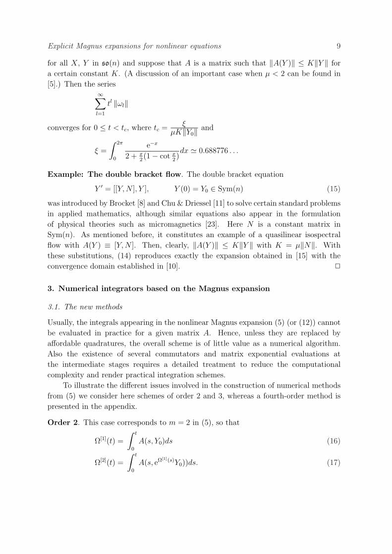
To illustrate the different issues involved in the construction of numerical methods
from (5) we consider here schemes of order 2 and 3, whereas a fourth-order method is
presented in the appendix.
Order 2. This case corresponds to m = 2 in (5), so that
Ω[1](t) =
∫ t
0
A(s, Y0)ds (16)
Ω[2](t) =
∫ t
0
A(s, eΩ[1](s)Y0))ds. (17)
Explicit Magnus expansions for nonlinear equations 10
If A is such that the integral (16) can be exactly computed, all that is required to get
a second order integrator is to replace the integral (17) with a quadrature rule of order
2. For instance, if we discretise Ω[2] with the trapezoidal rule, then
Ω[2](h) =h
2
(A(0, Y0) + A(h, eΩ[1](h)Y0)
)+O(h3). (18)
In fact, it is not necessary to evaluate exactly the integral (16), but only a first order
approximation. If, for instance, we use Euler’s method, Ω[1](h) = hA(0, Y0)+O(h2) and
this results in a new explicit second order scheme
v1 ≡ h
2
(A(0, Y0) + A(h, ehA(0,Y0)Y0)
)= Ω[2](h) +O(h3)
Y1 = ev1Y0, (19)
which is precisely the two-stage Runge–Kutta–Munthe-Kaas (RKMK) method with the
Butcher tableau
0
1 112
12
If, on the other hand, Ω[1] is discretised with Euler and Ω[2] with the midpoint rule,
v2 ≡ hA
(h
2, e
h2A(0,Y0)Y0
)= Ω[2](h) +O(h3)
Y1 = ev2Y0, (20)
we retrieve exactly the RKMK Heun method [17, p. 355].
Not all explicit RKMK methods can be recovered in this way and, moreover,
there are some interesting differences. In particular, RKMK methods always require
to discretise Ω[1] with a first-order quadrature, something not necessary for schemes
based on the preceding nonlinear Magnus expansion.
Order 3. In addition to eqs. (16) and (17) we have to work with
Ω[3](t) =
∫ t
0
(A2(s)− 1
2[Ω[2](s), A2(s)]
)ds, (21)
where A2(s) ≡ A(s, eΩ[2](s)Y0). If we use Simpson’s rule to approximate (21), then
Ω[3](h) =h
6(A(0, Y0) + 4A2(h/2) + A2(h))
− h
3[Ω[2](h/2), A2(h/2)]− h
12[Ω[2](h), A2(h)] +O(h4).
Now Ω[1] can be approximated with Euler and Ω[2](h) with the midpoint rule, eq.(20),
whereas
Ω[2](h
2) =
h
4
(A(0, Y0) +
h
4A(
h
2, e
h2A(0,Y0)Y0)
)+O(h3)
Explicit Magnus expansions for nonlinear equations 11
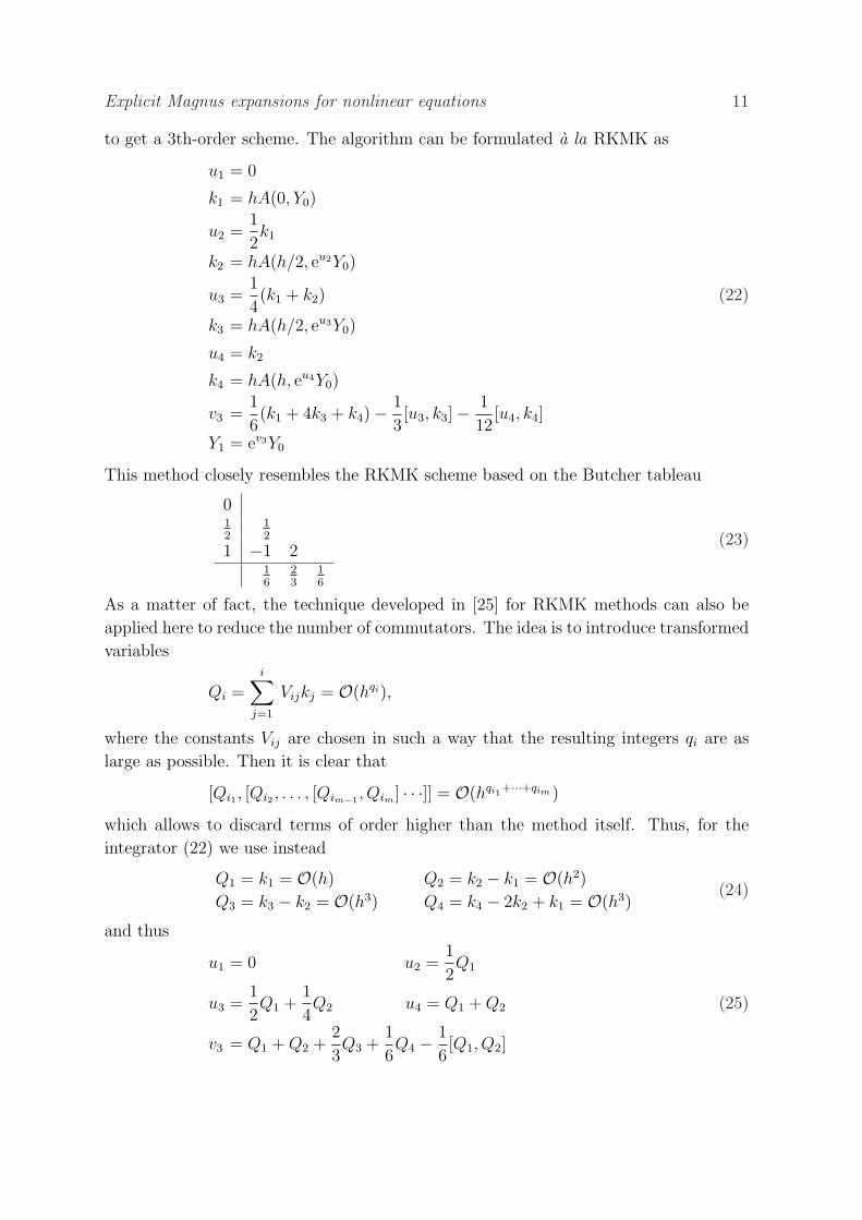
to get a 3th-order scheme. The algorithm can be formulated a la RKMK as
u1 = 0
k1 = hA(0, Y0)
u2 =1
2k1
k2 = hA(h/2, eu2Y0)
u3 =1
4(k1 + k2) (22)
k3 = hA(h/2, eu3Y0)
u4 = k2
k4 = hA(h, eu4Y0)
v3 =1
6(k1 + 4k3 + k4)− 1
3[u3, k3]− 1
12[u4, k4]
Y1 = ev3Y0
This method closely resembles the RKMK scheme based on the Butcher tableau
012
12
1 −1 216
23
16
(23)
As a matter of fact, the technique developed in [25] for RKMK methods can also be
applied here to reduce the number of commutators. The idea is to introduce transformed
variables
Qi =i∑
j=1
Vijkj = O(hqi),
where the constants Vij are chosen in such a way that the resulting integers qi are as
Explicit Magnus expansions for nonlinear equations 12
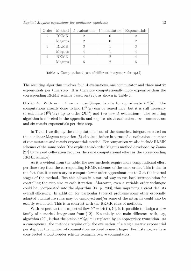
Order Method A evaluations Commutators Exponentials
2 RKMK 2 0 2
Magnus 2 0 2
3 RKMK 3 1 3
Magnus 4 1 4
4 RKMK 4 2 4
Magnus 6 2 6
Table 1. Computational cost of different integrators for eq.(2).
The resulting algorithm involves four A evaluations, one commutator and three matrix
exponentials per time step. It is therefore computationally more expensive than the
corresponding RKMK scheme based on (23), as shown in Table 1.
Order 4. With m = 4 we can use Simpson’s rule to approximate Ω[4](h). The
computations already done to find Ω[3](h) can be reused here, but it is still necessary
to calculate Ω[3](h/2) up to order O(h3) and two new A evaluations. The resulting
algorithm is collected in the appendix and requires six A evaluations, two commutators
and six matrix exponentials per time step.
In Table 1 we display the computational cost of the numerical integrators based on
the nonlinear Magnus expansion (5) obtained before in terms of A evaluations, number
of commutators and matrix exponentials needed. For comparison we also include RKMK
schemes of the same order (the explicit third-order Magnus method developed by Zanna
[27] by relaxed collocation requires the same computational effort as the corresponding
RKMK scheme).
As it is evident from the table, the new methods require more computational effort
per time step than the corresponding RKMK schemes of the same order. This is due to
the fact that it is necessary to compute lower order approximations to Ω at the internal
stages of the method. But this allows in a natural way to use local extrapolation for
controlling the step size at each iteration. Moreover, even a variable order technique
could be incorporated into the algorithm [14, p. 233], thus improving a great deal its
overall efficiency. In addition, for particular types of problems some other especially
adapted quadrature rules may be employed and/or some of the integrals could also be
exactly evaluated. This is in contrast with the RKMK class of methods.
With respect to the isospectral flow Y ′ = [A(Y ), Y ], it is possible to design a new
family of numerical integrators from (12). Essentially, the main difference with, say,
algorithm (22), is that the action euiY0e−ui is replaced by an appropriate truncation. As
a consequence, the methods require only the evaluation of a single matrix exponential
per step but the number of commutators involved is much larger. For instance, we have
constructed a fourth-order scheme requiring twelve commutators.
Explicit Magnus expansions for nonlinear equations 13
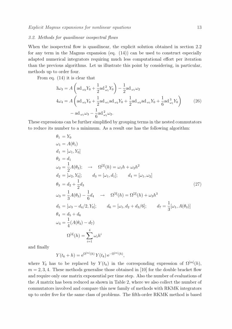
3.2. Methods for quasilinear isospectral flows
When the isospectral flow is quasilinear, the explicit solution obtained in section 2.2
for any term in the Magnus expansion (eq. (14)) can be used to construct especially
adapted numerical integrators requiring much less computational effort per iteration
than the previous algorithms. Let us illustrate this point by considering, in particular,
methods up to order four.
From eq. (14) it is clear that
3ω3 = A
(ad ω2Y0 +
1
2ad 2
ω1Y0
)− 1
2ad ω1ω2
4ω4 = A
(ad ω3Y0 +
1
2ad ω1ad ω2Y0 +
1
2ad ω2ad ω1Y0 +
1
6ad 3
ω1Y0
)(26)
− ad ω1ω3 − 1
6ad 2
ω1ω2.
These expressions can be further simplified by grouping terms in the nested commutators
to reduce its number to a minimum. As a result one has the following algorithm:
θ1 = Y0
ω1 = A(θ1)
d1 = [ω1, Y0]
θ2 = d1
ω2 =1
2A(θ2); → Ω[2](h) = ω1h + ω2h
2
d2 = [ω2, Y0]; d3 = [ω1, d1]; d4 = [ω1, ω2]
θ3 = d2 +1
2d3 (27)
ω3 =1
3A(θ3)− 1
6d4 → Ω[3](h) = Ω[2](h) + ω3h
3
d5 = [ω3 − d4/2, Y0]; d6 = [ω1, d2 + d3/6]; d7 =1
3[ω1, A(θ3)]
θ4 = d5 + d6
ω4 =1
4(A(θ4)− d7)
Ω[4](h) =4∑
i=1
ωihi
and finally
Y (tk + h) = eΩ[m](h) Y (tk) e−Ω[m](h),
where Y0 has to be replaced by Y (tk) in the corresponding expression of Ω[m](h),
m = 2, 3, 4. These methods generalise those obtained in [10] for the double bracket flow
and require only one matrix exponential per time step. Also the number of evaluations of
the A matrix has been reduced as shown in Table 2, where we also collect the number of
commutators involved and compare this new family of methods with RKMK integrators
up to order five for the same class of problems. The fifth-order RKMK method is based
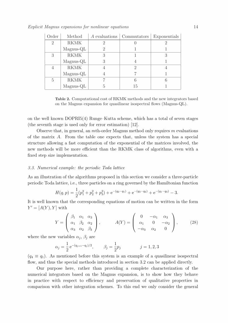
Explicit Magnus expansions for nonlinear equations 14
Order Method A evaluations Commutators Exponentials
2 RKMK 2 0 2
Magnus-QL 2 1 1
3 RKMK 3 1 3
Magnus-QL 3 4 1
4 RKMK 4 2 4
Magnus-QL 4 7 1
5 RKMK 7 6 6
Magnus-QL 5 15 1
Table 2. Computational cost of RKMK methods and the new integrators basedon the Magnus expansion for quasilinear isospectral flows (Magnus-QL).
on the well known DOPRI5(4) Runge–Kutta scheme, which has a total of seven stages
(the seventh stage is used only for error estimation) [12].
Observe that, in general, an mth-order Magnus method only requires m evaluations
of the matrix A. From the table one expects that, unless the system has a special
structure allowing a fast computation of the exponential of the matrices involved, the
new methods will be more efficient than the RKMK class of algorithms, even with a
fixed step size implementation.
3.3. Numerical example: the periodic Toda lattice
As an illustration of the algorithms proposed in this section we consider a three-particle
periodic Toda lattice, i.e., three particles on a ring governed by the Hamiltonian function
H(q, p) =1
2(p2
1 + p22 + p2
3) + e−(q2−q1) + e−(q3−q2) + e−(q1−q3) − 3.
It is well known that the corresponding equations of motion can be written in the form
Y ′ = [A(Y ), Y ] with
Y =
β1 α1 α3
α1 β2 α2
α3 α2 β3
, A(Y ) =
0 −α1 α3
α1 0 −α2
−α3 α2 0
, (28)
where the new variables αj, βj are
αj =1
2e−(qj+1−qj)/2, βj =
1
2pj j = 1, 2, 3
(q4 ≡ q1). As mentioned before this system is an example of a quasilinear isospectral
flow, and thus the special methods introduced in section 3.2 can be applied directly.
Our purpose here, rather than providing a complete characterization of the
numerical integrators based on the Magnus expansion, is to show how they behave
in practice with respect to efficiency and preservation of qualitative properties in
comparison with other integration schemes. To this end we only consider the general
Explicit Magnus expansions for nonlinear equations 15
0 0.5 1 1.5 2 2.5−8
−7
−6
−5
−4
−3
−2
−1
0
CPU time
erro
r
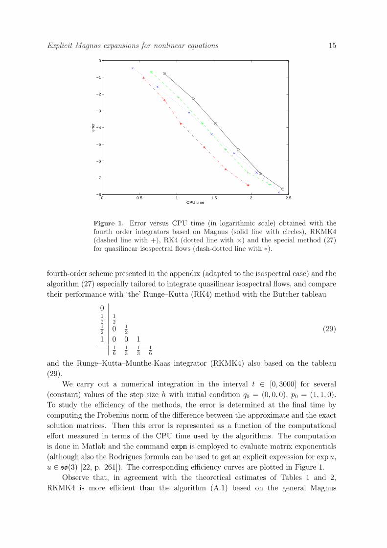
Figure 1. Error versus CPU time (in logarithmic scale) obtained with thefourth order integrators based on Magnus (solid line with circles), RKMK4(dashed line with +), RK4 (dotted line with ×) and the special method (27)for quasilinear isospectral flows (dash-dotted line with ∗).
fourth-order scheme presented in the appendix (adapted to the isospectral case) and the
algorithm (27) especially tailored to integrate quasilinear isospectral flows, and compare
their performance with ‘the’ Runge–Kutta (RK4) method with the Butcher tableau
012
12
12
0 12
1 0 0 116
13
13
16
(29)
and the Runge–Kutta–Munthe-Kaas integrator (RKMK4) also based on the tableau
(29).
We carry out a numerical integration in the interval t ∈ [0, 3000] for several
(constant) values of the step size h with initial condition q0 = (0, 0, 0), p0 = (1, 1, 0).
To study the efficiency of the methods, the error is determined at the final time by
computing the Frobenius norm of the difference between the approximate and the exact
solution matrices. Then this error is represented as a function of the computational
effort measured in terms of the CPU time used by the algorithms. The computation
is done in Matlab and the command expm is employed to evaluate matrix exponentials
(although also the Rodrigues formula can be used to get an explicit expression for exp u,
u ∈ so(3) [22, p. 261]). The corresponding efficiency curves are plotted in Figure 1.
Observe that, in agreement with the theoretical estimates of Tables 1 and 2,
RKMK4 is more efficient than the algorithm (A.1) based on the general Magnus
Explicit Magnus expansions for nonlinear equations 16
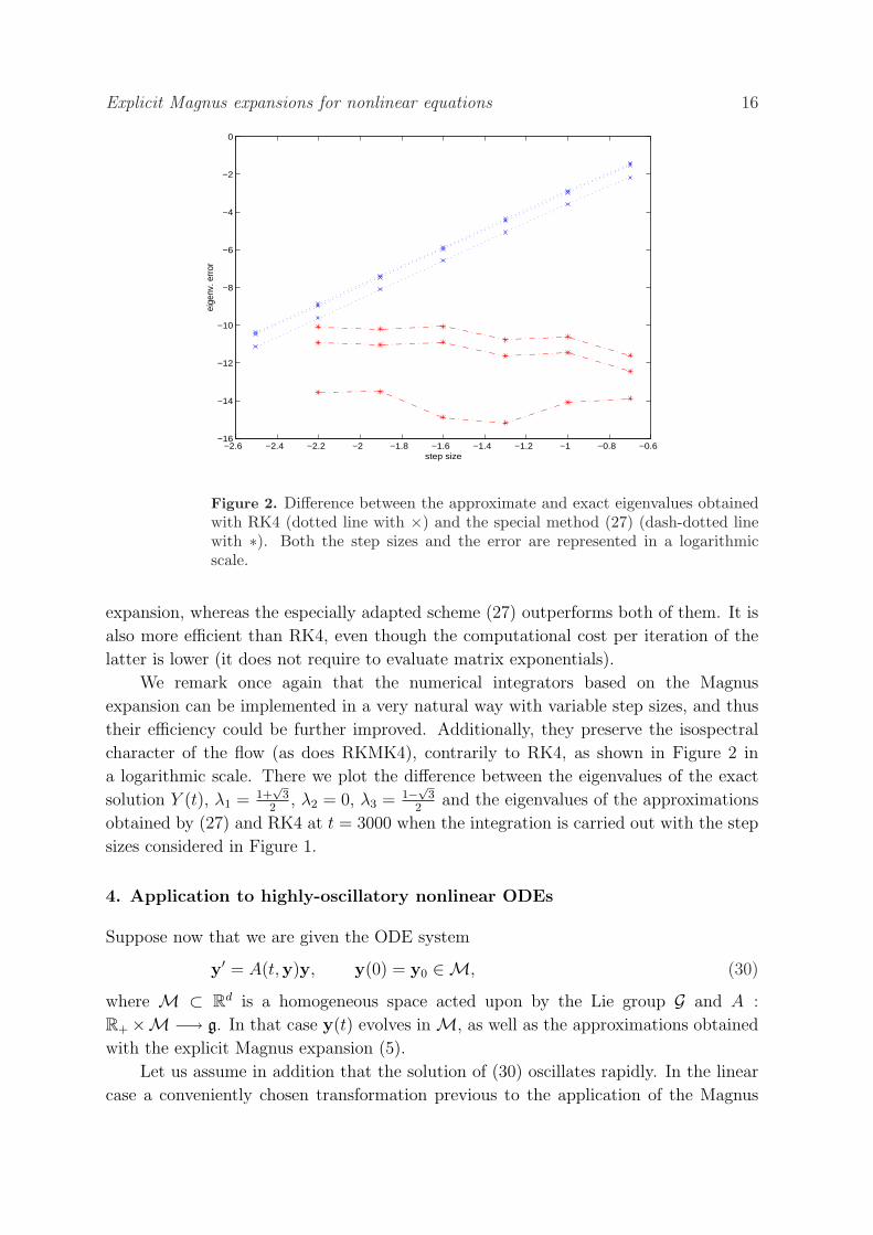
Figure 2. Difference between the approximate and exact eigenvalues obtainedwith RK4 (dotted line with ×) and the special method (27) (dash-dotted linewith ∗). Both the step sizes and the error are represented in a logarithmicscale.
expansion, whereas the especially adapted scheme (27) outperforms both of them. It is
also more efficient than RK4, even though the computational cost per iteration of the
latter is lower (it does not require to evaluate matrix exponentials).
We remark once again that the numerical integrators based on the Magnus
expansion can be implemented in a very natural way with variable step sizes, and thus
their efficiency could be further improved. Additionally, they preserve the isospectral
character of the flow (as does RKMK4), contrarily to RK4, as shown in Figure 2 in
a logarithmic scale. There we plot the difference between the eigenvalues of the exact
solution Y (t), λ1 = 1+√
32
, λ2 = 0, λ3 = 1−√32
and the eigenvalues of the approximations
obtained by (27) and RK4 at t = 3000 when the integration is carried out with the step
sizes considered in Figure 1.
4. Application to highly-oscillatory nonlinear ODEs
Suppose now that we are given the ODE system
y′ = A(t,y)y, y(0) = y0 ∈M, (30)
where M ⊂ Rd is a homogeneous space acted upon by the Lie group G and A :
R+×M −→ g. In that case y(t) evolves in M, as well as the approximations obtained
with the explicit Magnus expansion (5).
Let us assume in addition that the solution of (30) oscillates rapidly. In the linear
case a conveniently chosen transformation previous to the application of the Magnus
Explicit Magnus expansions for nonlinear equations 17
expansion allows to get very accurate results [16]. We generalize this approach to the
nonlinear setting.
Suppose that we have computed yn ≈ y(tn) and wish to advance to tn+1 = tn + h.
The idea is to consider a new variable z(x) such that
y(tn + x) = exA(tn,yn) z(x). (31)
Then
dz
dx= B(x, z(x))z, z(0) = yn (32)
with
B(x, z(x)) = F−1(x) [A(tn + x, F (x)z(x))− A(tn,yn)] F (x) (33)
and F (x) = exp[xA(tn,yn)]. We note for future use that B(0, z(0)) = O.
Observe that the new variable z(x) may also be seen as a correction to the solution
provided by the first order term Ω[1] of the Magnus expansion (discretized with Euler’s
method). For this reason one expects that if the system (32) is solved with the nonlinear
Magnus expansion the error in the corresponding approximations will be significantly
smaller than with the standard algorithm, even when the same quadrature rules are
used [16]. But in the highly-oscillatory case other specially tailored quadratures exist
which provide excellent results [19].
To illustrate the main features of the nonlinear modified Magnus expansion applied
to the highly-oscillatory system (30), let us consider equations of the form
where it is assumed that a(t, y, y′) À 1. Particular examples are the Emden–Fowler
(a = ty2), the Lane–Emden (a = (y/t)n−1) and the Thomas–Fermi (a = −(y/t)1/2)
equations [28].
When (34) is written in a matrix form, we obtain (30) with
A(t,y) =
(0 1
−a(t,y) 0
)
and y = (y, y′)T . Denoting by θn ≡√
a(t,yn), it is clear that
F (x) = exA(tn,yn) =
(cos xθn θ−1
n sin xθn
−θn sin xθn cos xθn
),
whereas for the new matrix B one gets, after some algebra,
B(x, z(x)) =1
4(θ2(x)− θ2
n)[2M1 + M2e
2iθnx + M3e−2iθnx
](35)
with θ2(x) ≡ a(tn + x, F (x)z(x)) and
M1 =
(0 −θ−2
n
1 0
), M2 =
(iθ−1
n θ−2n
1 −iθ−1n
), M3 =
(−iθ−1
n θ−2n
1 iθ−1n
).
Explicit Magnus expansions for nonlinear equations 18
This is the expression required for applying the nonlinear Magnus expansion (5). The
first term is given by
Ω[1](x) =
∫ x
0
B(τ,yn)dτ =1
2
∫ x
0
(θ21(τ)− θ2
n)dτ M1
+1
4
∫ x
0
(θ21(τ)− θ2
n)e2iθnτdτ M2 +1
4
∫ x
0
(θ21(τ)− θ2
n)e−2iθnτdτ M3
≡ I0(x)M1 + I+(x)M2 + I−(x)M3,
where now θ21(τ) ≡ a(tn +τ, F (τ)yn). Since B(0,yn) = O, any quadrature rule that uses
only the values of θ21(τ)− θ2
n at the endpoints requires only the value at x (the value at
the origin is zero). For the non-oscillatory part I0(x) we can use the trapezoidal rule
I0(x) ≈ xϕ1(x), with ϕ1(x) ≡ 1
4(θ2
1(x)− θ2n).
For I±(x) it seems appropriate to apply Filon–Lobatto quadratures. With this class of
methods one has in general∫ x
0
f(τ)e±2iθnτdτ ≈ b±1 (θn)f(0) + b±2 (θn)f(x)
with
b±2 (θn) =e±2iθnx
±2iθn
+e±2iθnx − 1
4xθ2n
.
Consequently, putting all the pieces together,
Ω[1](x) = ϕ1(x)(xM1 + b+
2 (θn)M2 + b−2 (θn)M3
)(36)
or equivalently
Ω[1](x) = ϕ1(x)
(cos 2θnx
θ2n
− sin 2θnx2θ3
nx− x
θ2n
+ sin 2θnxθ3n
− 1−cos 2θnx2θ4
nx
x + sin 2θnxθn
− 1−cos 2θnx2θ2
nx− cos 2θnx
θ2n
+ sin 2θnx2θ3
nx
).
For Ω[2](x) =∫ x
0B(τ, eΩ[1](τ)yn)dτ one gets the same expression (36), but now ϕ1(x) has
to be replaced by
ϕ2(x) ≡ 1
4(θ2
2(x)− θ2n), where θ2
2(x) = a(tn + x, F (x)eΩ[1](x)yn
).
Similar considerations apply to higher order terms, although the analysis is obviously
more involved. If the truncated Magnus solution of (32) is z(x) = exp(Ω[k](x))yn, the
approximation obtained in this way has the form
yn+1 = ehA(tn,yn) eΩ[k](h)yn, n ∈ Z.
5. Conclusions
The nonlinear Magnus expansion we have proposed in this paper can be considered
as a natural generalization of the usual expansion for linear problems. As well as
this, it provides explicit integrators in terms of integrals of nested commutators and
it is amenable to standard procedures to reduce the total number of commutators.
Explicit Magnus expansions for nonlinear equations 19
Although only methods up to order four have been presented here, the same strategy
can in principle be applied to construct higher order schemes preserving the main
qualitative properties of the exact solution. The new integrators require in general
more computational effort per time step than other well known Lie-group methods but
on the other hand they can be easily implemented with variable step sizes. Also, for
particular types of problems it is possible to adapt appropriately the procedure and
build up very efficient methods even with a fixed step size implementation.
In summary, this nonlinear Magnus expansion constitutes a very flexible tool to
analyse nonlinear equations defined on Lie groups and/or homogeneous spaces acted
upon by Lie groups. It allows to use different quadrature rules and even in some cases
to work with exact integrals. At the same time, the procedure can be modified to
cope with highly oscillatory systems of nonlinear ODEs in conjunction with especially
adapted quadratures.
Acknowledgments
The work of FC has been partially supported by Ministerio de Educacion y Ciencia
(Spain) under project MTM2004-00535 (co-financed by the ERDF of the European
Union) and Generalitat Valenciana (GV2003-002), while on sabbatical leave at the
University of Cambridge.
Appendix A.
In this appendix we present a 4th-order algorithm for the numerical integration of the
general Lie equation Y ′ = A(t, Y ) based on the nonlinear Magnus expansion (5) for
tn+1 = tn + h:
u1 = 0
k1 = hA(tn, Yn); Q1 = k1
u2 =1
2Q1
k2 = hA(tn +h
2, eu2Y0); Q2 = k2 − k1
u3 =1
2Q1 +
1
4Q2
k3 = hA(tn +h
2, eu3Y0); Q3 = k3 − k2
u4 = Q1 + Q2 (A.1)
k4 = hA(tn + h, eu4Y0); Q4 = k4 − 2k2 + k1
u5 =1
2Q1 +
1
4Q2 +
1
3Q3 − 1
24Q4 − 1
48[Q1, Q2]
k5 = hA(tn +h
2, eu5Y0); Q5 = k5 − k2
Explicit Magnus expansions for nonlinear equations 20
u6 = Q1 + Q2 +2
3Q3 +
1
6Q4 − 1
6[Q1, Q2]
k6 = hA(tn + h, eu6Y0); Q6 = k6 − 2k2 + k1
v = Q1 + Q2 +2
3Q5 +
1
6Q6 − 1
6[Q1, Q2 −Q3 + Q5 +
1
2Q6]
Yn+1 = evYn
Remarks:
(i) The computation of u5, k5 is independent of u6, k6 and it is required only to obtain
v (which differs from Ω[4](tn + h) only in O(h5) terms, that have no effect on the
order).
(ii) The above algorithm comprises also lower order methods: if we take v = k1 we
have a first-order scheme; if v = k2 then a second-order method results; finally, by
computing only up to u6 (but not u5, k5, Q5) we recover the third-order method
(22). It might be therefore implemented so that not only the step size but also the
order can be changed at each step, similarly to extrapolation methods [14, page
233].
(iii) This algorithm can also be directly applied to the isospectral flow Y ′ = [A(t, Y ), Y ]
with the replacement of euiYn by the action euiYne−ui in the computation of ki and
finally Yn+1 = evYne−v.
References
[1] S. Blanes, F. Casas, J.A. Oteo and J. Ros, Magnus and Fer expansions for matrix differentialequations: the convergence problem, J. Phys. A: Math. Gen. 31 (1998), pp. 259-268.
[2] S. Blanes, F. Casas and J. Ros, Improved high order integrators based on the Magnus expansion,BIT 40 (2000), pp. 434-450.
[3] S. Blanes, F. Casas and J. Ros, High order optimized geometric integrators for linear differentialequations, BIT 42 (2002), pp. 262-284.
[4] S. Blanes and P.C. Moan, Splitting metehods for non-autonomous Hamiltonian equations, J.Comput. Phys. 170 (2001), pp. 205-230.
[5] A.M. Bloch and A. Iserles, Commutators of skew-symmetric matrices, Intnl. J. Bifurcations &Chaos 15 (2005), 793–801.
[6] A.M. Bloch and A. Iserles, On an isospectral Lie–Poisson system and its Lie algebra, Universityof Cambridge Tech. Rep. DAMTP NA2005/01 (2005).
[7] A.M. Bloch, A. Iserles, J.E. Marsden and T.S. Ratiu, A class of integrable geodesic flows on thesymplectic group, in preparation.
[8] R.W. Brockett, Dynamical systems that sort lists, diagonalize matrices and solve linearprogramming problems, Linear Algebra Appl. 146 (1991), pp. 79-91.
[9] M.P. Calvo, A. Iserles and A. Zanna, Numerical solution of isospectral flows, Math. Comput. 66(1997), pp. 1461-1486.
[10] F. Casas, Numerical integration methods for the double-bracket flow, J. Comput. Appl. Math. 166(2004), pp. 477-495.
[11] M.T. Chu and K.R. Driessel, The projected gradient method for least squares matrixapproximations with spectral constraints, SIAM J. Numer. Anal. 27 (1990), pp. 1050-1060.
[12] J.R. Dormand, Numerical Methods for Differential Equations: A Computational Approach, CRCPress, Boca Raton (1996).
Explicit Magnus expansions for nonlinear equations 21
[13] E. Hairer, C. Lubich, and G. Wanner, Geometric Numerical Integration. Structure-PreservingAlgorithms for Ordinary Differential Equations, Springer Ser. Comput. Math. 31, Springer-Verlag, Berlin (2002).
[14] E. Hairer, S.P. Nørsett and G. Wanner, Solving Ordinary Differential Equations I 2nd Ed., SpringerSer. Comput. Math. 8, Springer-Verlag, Berlin (1993).
[15] A. Iserles, On the discretization of double-bracket flows, Found. Comput. Math. 2 (2002), pp.305-329.
[16] A. Iserles, On the global error of discretization methods for highly-oscillatory ordinary differentialequations, BIT 42 (2002), pp. 561-599.
[17] A. Iserles, H.Z. Munthe-Kaas, S.P. Nørsett and A. Zanna, Lie group methods, Acta Numerica 9(2000), pp. 215-365.
[18] A. Iserles and S.P. Nørsett, On the solution of linear differential equations in Lie groups, Philos.Trans. Royal Soc. London Ser. A 357 (1999), pp. 983-1019.
[19] A. Iserles and S.P. Nørsett, On quadrature methods for highly oscillatory integrals and theirimplementation, BIT 44 (2004), pp. 755-772.
[20] S. Klarsfeld and J.A. Oteo, Recursive generation of higher-order terms in the Magnus expansion,Phys. Rev. A 39 (1989), pp. 3270-3273.
[21] W. Magnus, On the exponential solution of differential equations for a linear operator, Commun.Pure Appl. Math. 7 (1954), pp. 649-673.
[22] J.E. Marsden and T.S. Ratiu, Introduction to Mechanics and Symmetry, Springer-Verlag, NewYork (1994).
[23] J.B. Moore, R.E. Mahony and U. Helmke, Numerical gradient algorithms for eigenvalue andsingular value calculations, SIAM J. Matrix Anal. Appl. 15 (1994), pp. 881-902.
[24] H. Munthe-Kaas, High order Runge–Kutta methods on manifolds, Appl. Numer. Math. 29 (1999),pp. 115-127.
[25] H. Munthe-Kaas and B. Owren, Computations in a free Lie algebra, Philos. Trans. Royal Soc.London Ser. A 357 (1999), pp. 957-981.
[26] H. Munthe-Kaas and A. Zanna, Numerical integration of differential equations on homogeneousmanifolds. In F. Cucker and M. Shub, editors, Foundations of Computational Mathematics,Springer-Verlag, Berlin, 1997, pp. 305-315.
[27] A. Zanna, Collocation and relaxed collocation for the Fer and the Magnus expansion, SIAM J.Numer. Anal. 36 (1999), pp. 1145-1182.
[28] D. Zwillinger, Handbook of Differential Equations 2nd Ed., Academic Press, Boston (1992).