1 Exploitation versus Exploration in Market Competition John Debenham University of Technology, Sydney [email protected]http://www-staff.it.uts.edu.au/~debenham/ Ian Wilkinson University of New South Wales [email protected]http://www.marketing.unsw.edu.au/people/html/IWilkinson.html Abstract A general simulation model of market competition is developed to explore the effectiveness of and interactions between different types product exploration and exploitation strategies i.e. innovation, imitation and process improvement. The model, like real markets, is highly non- linear such that analytical solutions in the form of optimal marketing strategies are not possible. Hence, we use simulation experiments to examine firm survival and the effectiveness of different strategy mixes and show how these depend on the length of time it takes for each strategy to bear fruit, the speed of new product diffusion and the duration of product life cycles and the timing of new product entry. The model is implemented on the Internet and provides the basis for further experiments to examine the impact of different combinations of firm strategies on survival and performance and as a means of honing management sensitivities regarding the impact of different market response functions on the outcomes of strategy. Introduction “It is the unending search for differential advantage which keeps competition dynamic” (Alderson 1957 p 102). With these words Wroe Alderson, one of the pioneers of modern marketing theory begins his discussion of the essential nature of the competitive process. Firms are continually seeking to create and deliver advantage or value to customers that are better than alternatives.
Transcript
1
Exploitation versus Exploration in Market Competition
Hence the profit for this time period, St–1i , is determined and so is the revenue that will be
carried over to the next time period. The “anti-clockwise loop” shown in Figure 2 goes “round
and round” from one time period to the next.
15
Budget
R
Output
Q
Costs
C
Profit
S = R – CPrice
Pj
Revenue
R = �j pj _ qi,j
See Fig 3.
t–1 i
carry over
R
carried over
R t–2 i
t–2 i
t–1 i
t–1 i
t–1 i
t–1 i
t–1 i
t–1 i
Figure 2. The model from the point of view of a particular firm i.
Figure 2 does not show how the carry over amount Rt–2i , available at the start of time period
[t – 1, t], generates output Qt–1i and costs Ct–1
i by the end of that time period. This is shown in
Figure 3. The horizontal dashed line in Figure 3 divides the figure into two time periods: [t–2, t–
1] in the upper part, and [t–1, t] in the lower part. First, the carry over amount Rt–2i from [t–2,
t–1] becomes the budget for the time period [t–1, t]. The budget Rt–2i is entirely committed to
hiring labour in the time period [t–1, t]. That is:
Lt–1i =
Rt–2i c
where c is the constant wage rate. For simplicity, c is set to unity. So a “unit of money” is the
cost of a unit of labour for one time period. Labour is split in the proportions wi : pi : mi : ni into
the four categories workers, process improvers, imitators and innovators. The imitators attempt
to build processes for producing products that have been discovered by other firms. If they are
successful then they create a level of manufacturing expertise, or process knowledge, that is
represented as a vector:
16
Imit–2i
For example:
Imit–2i = [0, 0, 1.0, 0, 0, 0, 0, 0,.....]
contains process knowledge with value 1.0 concerning product 3. The value 1.0 is added to the
third place of the firm’s process knowledge vector—this is described below. The value of a
firm’s process knowledge for a product will be 0.0 if the firm can not produce that product, and
1.0 if it has discovered how to produce that product by either innovation or imitation. The value
of the process knowledge may then be increased to an integer value greater than 1.0 by the firms
process improvers. The process improvers generate process knowledge for products that the firm
already produces.
A firm’s process improvers are allocated to improving the manufacturing processes for
particular products. The i’th firms process knowledge is denoted by a vector Ai. In the time
period [t – 1, t] the process improvers may have found new process knowledge Prot–1i —as for
Imit–2i this knowledge is represented as a vector denoting the product(s) that are the subject of
the generated process knowledge. Likewise the innovators Ni may discover process knowledge
for new products, Innot–1i . All knowledge generated during one time period may only be used in
subsequent time periods, and so each firms process knowledge available in the period [t – 1, t]
is:
At–1i = At–2
i + Imit–2i + Prot-2
i + Innot–2i
That is, each firms process knowledge accumulates from one time to the next. It remains to
describe how a firm’s workers use this knowledge. Firm i’s workers are distributed across the
range of products that the firm can produce as represented by the vector Wt–1i . [The way in
17
which this distribution is done is described below in the sub-section “Determining supply”.] The
quantity of output that the workers generate in the time period is:
Qt–1i = At–1
i _ Wt–1i
where the _ symbol means that the vectors are multiplied together element by element.
Total budget
R t–2 i
Innovators
Ni = n _ L t–1 i
t–1 i
Discoveries
Inno
Process specs
Pi = p _ L t–1 i
t–1 i
Process knowledge
Pro
Productivity
A t–1 i
Workers
W = w _ L t–1 i
t–1 i
Output
Q = A _ Wt–1 i
Costs
C = c _L t–1 i
t–1 i
Labour
L
t–1 i
t–1 i
carried over
Rt–2 i
[t – 2, t – 1]
[t – 1, t ]
t–1 i
t–1 i
t–1 i
t–1 i
Imitators
Mi = m _ L t–1 i
t–1 i
Copied knowledge
Imi t–1 i
Figure 3. An allocation of resources leads to output and costs for firm i. The dashed line separate two time periods, and dashed arrows mean that the new knowledge is not available until
the following time period.
18
The model in detail
Determining demand
The price of each type of product is determined at the end of each time period by the amount of
product generated in that time period, by the total amount of money available, and by the “relative
demand” for the different types of product which is determined by labour’s preferences. Relative
demand reflects the preferences of labour for different types of product. So a model of relative
demand for each product is required to calculate unit price, as is a model of supply—ie: the
product generated. Relative demand is considered now, and supply is considered in the next sub-
section.
A modified Bass model or penetration model (Fourt and Woodlock 1960; Mahajan, Muller,
and Bass 1990) with repeat purchase is used to model relative demand for different products in
the market subject to a fixed total overall market demand. The rate of new product diffusion the
rate of repurchase depends on the type of product or service, as numerous studies of new product
diffusion and adoption have indicated. Thus the rate of development of the demand for
automobiles is not the same as that for a new beverage because at best each member of the
population will purchase one or two automobiles but may purchase a beverage repeatedly. The
type of products that we have in mind in developing our model are packaged food products in a
market with fixed total demand. In each time period there is a total demand for a fixed s units of
product (eg: s packaged dinners). � is called the market size. Given a particular product (eg; a
particular packaged dinner), in a particular time period [t – 1, t], the initial penetration, Pt–1, is
the size of the population who has purchased this product at least once either during or before this
time period. In time period [t – 1, t], the first-time sales, Nt–1, are sales made of this product
during this period to those who have not purchased this product previously. Suppose that the
growth of initial penetration t is proportional, for some penetration constant �, to the size of the
19
population that has yet to purchase this product. Then initial penetration in time period [t – 1, t],
Pi, satisfies:
P0 = � _ ��
P1 – P0 = � _ (� – P0)�
P2 – P1 = � _ (� – P1)�
Or as a continuous approximation:
dPdt = � _ [ � – P ]
Solving this differential equation gives the initial penetration:
Pt = � _ (1 – exp( – � t ) )
First-time sales is the rate of change of initial penetration. So if Nt is first time sales at time t:
Nt = Pt – Pt–1
and as a continuous approximation:
Nt = dPt
dt = � _ � _ exp( – � t ) ) (1)
First-time sales for a market of size � = 100 and penetration constant 0.1 is shown in Figure 4.
Figure 4. First-time sales, Nt, for a market of size 100 and � = 0.1.
20
Now suppose that once labour has purchased a product, labour continues to purchase that
product with a probability of �. That is, if Ti is total sales in time period [i – 1, i]:
Ti+1 = Ni+1 + � _ Ti
where Ni is first time sales in time period [i – 1, i]. Then:
T0 = N0
T1 = � _ N0 + N1
T2 = �2 _ N0 + � _ N1 + N2
etc
Or as a continuous approximation:
Tt = ∫ i=0t �t–i _ Ni _ di
Evaluating this using equation (1):
Tt = � _ �
ln(�� + � _ [ �t – exp(–t _ �) ](2)
Which, for a market size of � = 100 gives total sales values for each time period as shown in
Figure 5 for various � and �. The sales graphs in Figure 5 are now used to model relative
demand. The discovery of a new product by an innovating firm can lead to a substantial shifts in
demand for different firm’s products, depending on how rapidly the new product diffuses through
the market and the peak demand achieved, which depend on the values of the parameters � and �.
For example, with � = 0.2 and � = 0.9, there is a rapid growth in demand for a new product to
nearly 50% share within 8 time periods. The choice of � and � in the simulations described
below substantially effects the speed and extent of new product diffusion and the duration of the
life cycle of the product, as can be seen from the illustration in Figure 5. This affects the results
of firm’s using different strategies as we will show.
21
� = 0.05 and � = 0.4
� = 0.05 and � = 0.7
� = 0.05 and � = 0.9
� = 0.1 and � = 0.4
� = 0.1 and � = 0.7
� = 0.1 and � = 0.9
� = 0.2 and � = 0.4
� = 0.2 and � = 0.7
� = 0.2 and � = 0.9
Figure 5. Total sales for each time period for a market of size � = 100 and various � and �. For a given market size �, equation (2) has two variables: � and �. Given the values of a total sales function in the first two time periods, f0 and f1, it is easy to calculate � and �:
� = f0
�
� = f1 f0 –
� – f0
�
and so knowing the first two values of a total sales function is to know “all there is” about it.
22
Returning now to the problem of modelling relative demand. The general shape of the total
sales function in Figure 5 is a fair description of how interest in a new product, such as packaged
foodstuffs, might be expected to develop. Equation (2), for some values of � and � is used here
to model relative demand. So each product has a relative demand determined by equation (2),
with its own values of � and �, for some fixed arbitrary �, say, � = 1. Consumers distribute their
money over the different products in proportion to their relative demand D for each product as
described above. The prices per unit of the products is in proportion to their relative demand,
and are set so as to clear the market.
Determining supply
The only flexibility that a firm has is first to choose its parameters: wi, pi, mi and ni, and second
to decide what products its workers should produce. This second question is considered now. At
the beginning of each time period each firm knows all about the relative demand for the products
that it is able to produce. A rational choice of which product to produce in which quantities may
not be obvious. For example, consider the choices in the illustrations shown in Figure 6—all of
which were produced using equation (2). In (a) and (b) the function that appears to be the most
valuable turns out not to be by time 6 or 7. In (c) the function that appears to be the most
valuable remains so until time 28—so choosing between those two functions is not simple as the
choice will depend on whether anything “interesting” occurs between time 1 and time 28.
(a) (b) (c)
Figure 6. Choosing output on the basis of relative demand.
23
Suppose a firm has to choose between two products such as those whose relative demand
functions are shown in any of the three pairs in Figure 6. Consider Figure 6(a) in which the
graphs cross at time 6: a rational decision could be to produce the product with the higher relative
demand up to time 6 and then to change to the product with higher demand after time 6. But if a
firm were to behave in this way then the second product function should have been drawn starting
at time 6. Some simplifying assumption is required to prevent these considerations from over-
complicating this investigation. After all, the objective of this investigation is to explore changes
in performance resulting from modification of the four basic parameters. So each firm in the
simulations will produce all of the products for which it possesses process knowledge, and will
do so in quantities proportional to their relative demand.
Analysis
Innovation and Trading Off Exploration and Exploitation
Suppose a number of identical firms commence production of a range of products at the same
time, and each produces their air share of products —as described in the previous sub-section. As
time passes the relative demand of each product will rise and then decline as determined by (2),
as illustrated for a number of different values of � and � in Figure 5. If the firms manage the
production of their respective products in the same way then their market share will remain the
same; customers (labour), on the other hand, will become less enthusiastic about purchasing the
products but will continue to do so as there is no choice.
This situation is reminiscent of collusive oligopoly that operate through an informal “wink
and a nod” or by some, possibly illegal, collusive agreement. This state of affairs will be
perturbed if one of the firms discovers a new product. Initially the relative demand of this new
product may rise well above that of the established products whose product life cycles may now
24
be well into their decline stages. On introduction of this new product the innovating firm will
benefit by being a monopolist and gain from the demand for this new product, but monopolistc
pricing strategies are ruled out by our market clearing price system.
But, innovation comes at a price. In order to innovate, the i’th firm must allocate some of its
labour to innovation by setting ni > 0. Suppose that two firms commence production of the
same, single product at the same time. Suppose that the first firm allocates all of its labour as
workers, w1 = 1, and that the second firm divides its labour equally between workers and
innovators, w2 = n2 = 0.5. The role of the innovators in the second firm is to discover a new type
of product, and, until they do, they contribute nothing. If the innovators fail to discover a new
type of product then the size of the second firm will decline. Suppose that both firms initially
have 100 units of labour that are paid one unit of money each per time period, and suppose that
each firm's process knowledge is 1.0 for each product. At the end of the first time period the first
firm will produce 100 units of product and the second firm 50. So two thirds of the revenue of
200 will go to the first firm and one third to the second. In the second time period the first firm
will employ 133 units of labour and the second firm 67. The continuing development of their
respective sizes is shown in Figure 7. In nine time periods the second firm is less that one per
cent of its original size. However, if the second firm had set w2 = 0.9 and n2 = 0.1 then it would
have taken 52 time periods for the size of the firm to become less than one per cent of its original
size. In general if Lt–12 is the size of the second firm at the end of time period [t – 1, t] then:
Lt2 =
TR _ (1 – n2) _ Lt–12
TR – (Lt–12 _ n2)
where TR is the total revenue, ie: 200 in the example above. One advantage of defining relative
demand using equation (2) is that a firm can only go out of business “analytically” by choosing to
have no workers; ie: by setting wi = 0. The size of the firm illustrated in Figure 7 becomes
smaller and smaller without actually reaching zero.
25
Figure 7. The development of the sizes of a non-innovator firm and an innovator firm each of which has an initial size of � = 100. The innovator firm allocates 50% of its labour to
innovation, fails to discover a new product and dies.
Suppose that the second, innovating firm discovers a new product in time period 10. This
may or may not be a good thing in the medium term as Figure 8 illustrates. Even if a new product
is valuable, an innovating firm may find that it is so depleted that it is unable to produce sufficient
quantities to benefit from this new product in the medium term. The problem here is classic
tradeoff between exploration and exploration. . It is a problem of trading off the future benefits
to exploration, in this case innovation, against the more immediate benefits of greater exploitation
of the demand for existing products, i.e. devoting more resources to producing current products.
The tradeoff in turn depends on the timing of new product discoveries and the speed and size of
the market that will result. For example, Figure 7 shows that setting ni = 50% results in a firm
having no resources left to exploit the results of its innovation.
26
Figure 8. Two new products introduced at time 10—the figure shows the relative demand of the three products.
In rough terms, we think of a time period as being one week. The rate at which the i’th firm
can expect to discover a new product will depend on the amount of person-hours spent on
innovating, and this will depend on both its total labour force and on the proportion of its labour
force allocated to innovation, ni. For example, suppose that at the beginning there are two firms
that have the same size and that the first firm sets w1 = 1, and that the second sets w2 = 0.9 and
n2 = 0.1. If the mean of the random discovery process is twenty weeks then by time 20 the
second firm will be 23.8% of its original size—by time 30 it would have shrunk to 9% if its
original size.
The trade-off between innovation and exploiting the demand for existing products depends on
the speed and amount of market penetration for new products, as well as the time between new
product discoveries noted already. This can lead to first mover advantages and disadvantages, as
is illustrated in the following example.
First Mover Effects
Suppose two firms start at time zero each producing a product with � = 0.1 and � = 0.8, and
that in time period [20, 21] the second firm discovers a new product with the same � and �. The
relative demand curves are shown in Figure 9(a). From time 21 onwards the second firm will
produce the original product and its new product in quantities that are proportional to their
27
relative demand—as described above. How will the second firm fare? Not badly it would seem,
as is shown in Figure 9(b). The second, innovating firm’s size reaches a low of 19 in time period
[21, 22] and then turns up quite sharply reaching 99.6% of the labour force by time period
[29, 30]. The first, non-innovating firm has virtually been obliterated by time 40. The problem
for the first firm is that the second firm has a new product whose relative demand remains above
that of the only product that the first firm can produce. Thus innovation is rewarded.
However, both firms may survive depending on the pattern and size of diffusion of the new
product. Figure 10 shows the results for a market in which the parameter settings for the original
product's demand function are � = 0.1 and � = 0.8 and for the new product for the second firm
they are � = 0.2 and � = 0.7. Under these conditions, by time 200 the beneficial effect of the
second, innovating firm’s new product has passed and it is obliterated. The reason for this being
that the graphs in Figure 10(a) cross at time 45, after which the original product has a higher
relative demand, but the second firm continues optimistically to make a mix of both products.
What happens within 200 time periods is shown in Figure 10(b).
(a)
(b)
Figure 9. For two firms a new product with � = 0.1 and � = 0.8 is introduced at time 20. (a)
shows the resulting relative demand of the two products and (b) shows the resulting sizes of the
two firms.
28
(a)
(b)
Figure 10. For two firms a new product with � = 0.2 and � = 0.7 is introduced at time 20. (a) shows the resulting relative demand of the two products and (b) shows the resulting sizes of the
two firms.
Clearly, the benefits of a new product must be great enough to allow the innovating firm to
recover its investment. The insight from the simulation is how this depends on the timing of the
new product introduction and from the pattern of growth of demand over time of the new product
relative to existing products. In Figure 10, if the new product entered later it would sustain its
superior demand over the existing product for longer but this would be at the cost of increased
investment in innovation. In a later section we examine in more detail the return on investment
from different types of strategies and how this is depicted in the simulation results.
In the simulations described here, a firm discovers an innovation when the total amount of its
labour periods allocated to innovation reaches an innovation target. The innovation target may
be a fixed amount or may be randomly determined in some interval. Once a firm has discovered
an innovation, its “innovation counter” is decreased by the amount of the innovation target for the
next discovery.
If two innovating firms are competing then what is the optimal value of ni? This will depend
on the values of �, � and the innovation threshold. These proved difficult to calculate. Perhaps
this is due to computational round-off errors, or perhaps there are only “approximate” optima.
29
These matters are not resolved here and await further research investigation. The optimal
percentage to allocate to innovation, for various innovation thresholds and different values of the
two demand parameters, are shown in Table 1. The table shows us that the higher the innovation
threshold the greater the percentage of resources that should be devoted to innovation. It also
shows that the more rapid and greater is product diffusion [see Fig 5] the lower the optimal value
for the innovation allocation ni. The latter result occurs because there is more to be gained (and
hence lost) by focusing resources on exploiting the demand for existing products or any new
product developed than there is to devoting resources for developing new products.
Table 1. Optimal values of ni for values of innovation threshold between 20 and 100 where � =
0.1 and � = 0.7.
Imitation and Trading Off Exploitation and Exploration
The kind of imitation described here is that of using labour to copy new products introduced by
other firms, rather than, say, purchasing technology from other firms. So if a firm allocates
resources to imitation then they can only be employed as imitators if there is a product in
production that their firm can not produce. If a firm allocates resources to imitation then those
resources are re-applied to the worker category until a new product is discovered when the
imitation allocation is fully applied to imitation until the required knowledge is found. On
31
observing a new product discovered by another firm the imitators work until they can produce
that product, at which time it becomes an output of their firm with a process knowledge value of
1.0. As for innovation, imitations are discovered when the total amount of its labour periods
allocated to imitation reaches an imitation target. The imitation target may be a fixed amount or
may be randomly determined in some interval. Once a firm has discovered an imitation, its
“imitation counter” is reduced by the imitation target value for the next discovery. There is little
to be gained by investing in imitating a product if that product’s relative demand is low. Figure 6
shows that selecting the “best” relative demand function is not simple. For want of a better
criterion, an imitating firm will choose the most recently discovered product to attempt to imitate.
If two imitating firms are competing then what is the optimal value of mi? For this to make
sense at least one firm needs to be innovating, as otherwise there will be nothing to imitate. If
neither firm is innovating then all of the products in the system are those that were there at the
beginning. So the reward for a firm that invests in imitation will be products that are as old as the
products that it already has. Unless the relative demand functions for the imitated products are
significantly different from those of its existing products such an investment will not be worth
while. If the relative demand functions of all products are the same then imitation is certainly not
worth while. So the question of an optimal value of mi only really makes sense if both of the
firms are innovating. Consider two firms, each of which allocates an optimal 7% to innovation
with an innovation threshold set at 70.0—as indicated in Table 1, � = 0.1 and � = 0.7. The firms
now allocate differing proportions of staff to imitation for different values of the imitation
threshold.
The result is zero even for small values of the imitation threshold. It appears that if a firm
allocates the optimal proportion of its resources to innovation, ni, then imitation is not worth
doing. Therfore we consider what happens if two firms have an identical, sub-optimal allocation
to innovation and different allocations to imitation. Suppose that both firms allocate 4% to
32
innovation [threshold 70] and different amounts to imitation [threshold 20]. A local optimal
imitation allocation is around 8%—which does better than 7% and 9%. But 0% does better than
the 8%! It seems that if two firms are both innovating to the same extent then imitation is not
worth while—it is better to allocate resources to the generation of new products. But this does
not mean that imitation is not worth while generally. Below we show that, under certain
circumstances, an imitating firm can live off an innovating firm.
A related question is the level of imitation that leads to the slowest decline. If two firms
allocate 6% to innovation [threshold 70], with he first allocating 0% to imitation [threshold 5],
then 22% allocated to imitation for the second firm leads to the slowest decline with the firm’s
size at 0.2% of its original size at time 100. This is slower even than allocating a very small
amount to imitation, say 0.1%. The reason for this is not clear to us at present and serves as a
demonstration of the sometimes non-intuitive outcomes of nonlinear systems behaviour that
Robert May (1976) describes.
Process improvement: Trading off further exploitation
Investment in process improvement enables a firm to produce output at lower cost. Each firm has
a level of process knowledge for each product. Firm i’s workers are distributed across the range
of products that the firm can produce as represented by the vector Wt–1i . The quantity of output
Qt–1i that the workers generate in the time period is:
Qt–1i = At–1
i _ Wt–1i
where At–1i is the firms process knowledge, and _ means that the vectors are multiplied together
element by element. Each firm’s process knowledge for a given product either remains constant
or increases from one time to the next. Initially the process knowledge is set to 1.0 in which case
“one worker will produce one unit of product in one time period”. If a firm allocates labour to
33
process improvement then it is reasonable to allocate those process improvers to (one of) the most
recent product(s) that the firm has learned to produce. In this way an improving firm will derive
returns from such investments for products whose relative demand is likely to be large. In any
case, this makes sense as the more recent the product the greater the likelihood of deriving benefit
from investing in process improvement for that product.
The model chosen for process improvement is similar to that chosen for both innovation and
imitation. That is, an investment of a certain proportion of labour on the improvement of a
particular product until the labour/time exceeds a set improvement threshold will cause the
process knowledge for that product to increase by one. The reason for this choice is to ensure a
uniform basis for innovation, imitation and improvement. For example, if two firms are both
producing their own single product with the second firm allocating 10% of its labour to process
improvement, then this leads to an initial decrease in the size of the second firm. Figure 11(a)
shows what happens with a process improvement threshold of 50—the two graphs cross in time
period [33, 34]. Figure 11(b) shows a threshold of 100. These calculations are invariant to the
values of alpha and gamma.
(a)
(b)
Figure 11. Two firms with an initial size � = 100, the second firm allocates 10% of its labour to process improvement. In (a) with a process improvement threshold of 50, and in (b) with a
process improvement factor of threshold of 100. If two improving firms are competing then what is the optimal value of pi? Suppose that two
firms allocate 5% to innovation [threshold 70]. Then the more allocated to improvement
34
[threshold of 20] the better, up to 30% when a difference of 5% is not sufficient to dominate
within 160 time units although the equilibrium reached is alarmingly unstable. See Figure 12.
Figure 12. Two firms with an initial size � = 100, both firms allocate 5% to innovation
[threshold 70], the first firm allocates 30% to improvement [threshold of 20] and the second firm
allocates 25%.
The Return on Investment of Different Strategies
The return on investment (ROI) of different strategies may be indicated in terms of the area
beneath the relative demand curve for a product. For example an innovator invests for a period of
time and discovers a new product. That directly benefits the innovator until an imitator learns to
imitate that product, at which time the innovator will share the benefit with the imitator. The
innovators relative benefit is shown as the hashed area in Figure 12(a). Likewise the imitators
relative benefit is shown in Figure 12(b).
(a) innovator (b) imitator (c) improver
Figure 12. Return on investment for an innovator, an imitator and an improver.
35
If an innovating firm is competing with an imitating firm then, when the innovating firm
discovers a new product, it benefits entirely from the revenue derived from selling that product
until the imitating firm learns how to produce that product and thereafter the two firms share the
revenue from that product. So the difference between the sales volumes derived by the
innovating firm and the imitating firm is related to the area beneath the being-imitated product’s
relative demand curve from its beginning to the time at which the imitating firm learns how to
imitate that product. The area beneath a relative demand curve (2) from the beginning to time t
is:
∫ x=0t
� _ �ln(�� + � _ [ �x – exp(–x _ �) ] _ dx
= � _ �
ln(�) + � _ [ �t
ln(�) + exp(– t _ �)
� –
1ln(�) –
1� ] (4)
which gives an area under the entire curve of:
� _ �ln(�) + � _ [ –
1ln(�) –
1� ]
For example if � = 0.1 and � = 0.7 then the area under the entire curve is 448.142, and the
expression (4) tends asymptotically to this value.
The process improver will invest in improving production for a recently discovered, or
copied, product. When the investment in process improvement exceeds the improvement
threshold the process knowledge for that product will increase by 1.0. This is illustrated in Figure
12(c).
What Figure 12 shows is that if an innovating firm, an imitating firm and an improving firm
are coexisting in a moderately stable way then we expect the innovation threshold to be greater
than the process improvement threshold, which in turn will be greater than the imitation
threshold. This turns out to be the case.
36
Model Constraints
Before continuiing with the analysis some necessary constraints on model parameters needs to be
explained. .The first constraint on the parameters follows from the use of discrete time in the
simulations. The constraint is that each firm can have at most one of each of innovation,
imitation and improvement in any time interval. To ensure that this constraint is satisfied it is
sufficient to ensure that the product of the total labour and the percentage allocated to each of
endeavour is less than the threshold for that endeavour. For example, if the total labour is 200,
and a firm allocates 10% to imitation then the imitation threshold must be greater than 20.
The model economy described here is fundamentally unstable due to the shape of the relative
demand curves which when an innovation, imitation or improvement is found may substantially
increase the fortunes of the firm involved. This suits our purpose which is to investigate the,
consequently fairly rare, regions of stability.
The next constraint is to ensure that the alpha and gamma parameters are chosen so that these
regions of stability are not too small. This can be achieved by ensuring that when an innovation
is made by a firm the relative demand curve of the most recent existing product for that firm does
not declined to a level that threatens the survival of the firm. Otherwise Innovators would go out
of business before any innovation ever occur. For example, suppose that the steady state size of
firms is 100, and that the innovation threshold is 100 then a firm that allocates 10% of its labour
to innovation can be expected to discover an innovation approximately every ten time units. If
� = 0.1 and � = 0.7 then the relative demand curve has the shape shown in Figure 5. Those
diagrams show time extending from zero to 50. So a new innovation made at ten to fifteen time
units would occur when the previous innovation’s curve is well past its peak but still sufficient to
permit the innovator to survive.
We also attempt to ensure that the alpha and gamma parameters are chosen so that the regions
of stable coexistence of different types of strategies are not too large. This can be achieved by
37
ensuring that when an innovation is made by a firm the relative demand curve of the most recent
existing product for that firm “has decayed a fair amount”. By “a fair amount” we mean that an
innovating firm will not discover a new product before the relative demand curve of its
“previous” new product reaches its maximum value. Setting the derivative with respect to t of
equation (2) to zero:
tmax = 1
ln(�) + � _ ln( – � ln(�) ) (3)
The values of tmax for the nine relative demand curves illustrated in Figure 5 are given in Table 2.
In so far as the maximum value of the relative demand curve is useful for determining
“interesting” values for innovation effort, the values in Table 2 can be used as a guide. For
example, suppose that a firm has a product whose relative demand curve has � = 0.1 and � = 0.7,
suppose that this firm has initial size � = 100 and 10% of its labour allocated to innovation. If the
innovation effort is set at 50, or there abouts, and if the imitating firm’s size remains at its initial
value, then the imitating firm will discover how to make the product when the relative demand
curve of its old product is at its peak.
�
tmax 0.4 0.7 0.9
0.05 3.357 6.407 13.464
� 0.1 2.714 4.954 9.741
0.2 2.125 3.692 6.772
Table 2. Values of tmax for various values of � and �.
What is a “good” value for the innovation target when, say, � = 0.1 and � = 0.7? This
function is illustrated in Figure 5. If the innovation target is high then by the time a new product
is discovered the relative demand of the “old” products will be very low and so the impact of the
38
new product will be large and destabilising. These experiments address destabilising effects, but
if they are too great then the location of the stability points is very sensitive. The relative demand
curve for � = 0.1 and � = 0.7 reaches a maximum value of 17 at about time 5. By time 13 it has
dropped back to around 10, and by time 35 it has dropped back to around 1.18. So if a firm were
to discover a new product at time 35 then the new product would be competing with an old
product whose relative demand was around unity and falling—highly unstable behaviour would
result. As a general rule if the time to discover a new product is greater than “lower teens” then
highly unstable performance should be expected.
Interactions Between Innovation, Imitation and Process Improvement Strategies
The interplay between imitation, innovation and improvement is quite complex. For example
consider three firms—the first allocates 10% of its labour to innovation, the second 15% to
imitation, and the third 5% to each of imitation and improvement. The innovation effort
threshold is set at 80, the imitation threshold at 20, and the improvement threshold at 30. All
products have � = 0.1 and � = 0.7. Then:
• Firm 1 has an initial product number 0
• Firm 2 has an initial product number 1
• Firm 3 has an initial product number 2
• Firm 3 starts improving product number 2 in time interval [0,1] process knowledge = 1.0
• Firm 2 starts imitating product number 2 in time interval [0,1]
• Firm 3 starts imitating product number 1 in time interval [1,2]
• Firm 2 discovers how to imitate product number 2 in time interval [2,3]
• Firm 2 starts imitating product number 0 in time interval [3,4]
• Firm 2 discovers how to imitate product number 0 in time interval [5,6]
• Firm 3 discovers how to imitate product number 1 in time interval [8,9]
39
• Firm 3 discovers how to improve product number 2 in time interval [9,10] process
knowledge = 2.0
• Firm 3 starts imitating product number 0 in time interval [9,10]
• Firm 3 starts improving product number 1 in time interval [10,11] process knowledge = 1.0
• Firm 1 discovers a new product number 3 in time interval [13,14]
• Firm 2 starts imitating product number 3 in time interval [14,15]
• Firm 3 discovers how to imitate product number 0 in time interval [15,16]
• Firm 3 discovers how to improve product number 1 in time interval [16,17] process
knowledge = 2.0
• Firm 3 starts imitating product number 3 in time interval [16,17]
• Firm 3 starts improving product number 0 in time interval [17,18] process knowledge = 1.0
• Firm 2 discovers how to imitate product number 3 in time interval [17,18]
• Firm 3 discovers how to imitate product number 3 in time interval [19,20]
• Firm 3 discovers how to improve product number 0 in time interval [24,25] process
knowledge = 2.0
and the resulting firm sizes are shown in Figure 13.
Firm 1 Firm 2 Firm 3
Figure 13. Three firms with an initial size of 100, the first firm allocates 10% of its labour to innovation, the second allocates 15% to imitation, and the third allocates %5 each to imitation
and improvement with , � = 0.1 and � = 0.7 for all products. The innovation effort threshold is set at 80, the imitation threshold at 20, and the improvement threshold at 30.
The model allows us to explore the conditions under which firms in a market adopting
different exploitation and exploration strategies can survive and when they do not. When different
40
firms can coexist for long periods of time we can define the market as stable. For the purposes of
analysis we will define a market as stable if all firms are still in business at time 250. This is a
very pragmatic definition but, given the tendency of the system to destabilise, it is quite
reasonable. For example, consider two firms. The first firm allocates 10% of its labour to
innovation, and the second 5%. Suppose the innovation threshold = 40, � = 0.1 and � = 0.7.
How much should the second firm allocate to imitation if it is to compete with the first? The
answer is none. Why? Table 1 shows that the optimal value for ni with these parameters is 4.9.
So the second firm will dominate the first without any investment in imitation. By time 45 the
size of the first firm is practically zero.
Now consider two firms where the first allocates 5% to innovation and the second 5% to
imitation. Given a value of the innovation threshold, what values for the imitation threshold lead
to joint survival? That is, under what circumstances can an imitating firm “live off” an
innovating firm? The result may at first appear counter-intuitive in that as the innovation
threshold increases the stable imitation threshold decreases. The reason for this is that in a stable
configuration the imitation threshold should be at a level so that the imitating firm discovers how
to imitate in good time but not too soon. If it discovers an imitation early in the innovation cycle
then it will have nothing else to imitate and so will allocate all of its labour to workers and so
may kill the firm from which it derives its inspiration. Further, the greater the innovation
threshold the longer the time between innovation discoveries, the greater the relative demand of
the discovered product, and the sooner the imitator imitator must learn to imitate the product.
Table 3 shows sample values and Figure 15 shows the respective sizes of the firms—the imitating
firm dominates.
41
Innovation threshold Imitation threshold
10.0 9.6762085
15.0 10.123603
20.0 9.366529
25.0 8.693429
30.0 7.92837
35.0 7.215324
40.0 6.624544
45.0 6.3362412
50.0 5.8482556
55.0 4.824529
60.0 4.6543684
65.0 4.5592747
70.0 4.454127
75.0 4.164027
Table 3. Optimal values of the imitation threshold for values of the innovation threshold
between 10 and 75 where two firms invest 5% in innovation and imitation respectively, and � =
0.1 and � = 0.7.
Figure 15. Two firms compete. An innovating firm allocates 5% to innovation with a threshold 40, an imitating firm allocates 5% to imitation with a threshold at 6.624544. There is no
randomisation of the parameters: � = 0.1, � = 0.7 and � = 100. Next consider two firms where the first allocates 5% to innovation and the second 5% to
improvement. Given a value of the innovation threshold, what values for the improvement
42
threshold lead to joint survival? That is, under what circumstances can an improving firm survive
against an innovating firm? The improving firm will be making further and further
improvements to its production of the one product that it knows how to produce. It is no surprise
that the stable values are very hard to find—a very small change alters the outcome completely.
Table 4 shows sample values and Figure 16 shows the respective sizes of the firms—the
innovating firm dominates. The graph in Figure 16 shows sizes up to time 50 only and is not
stable—locating the stable solution is very time consuming and probably beyond double precision
arithmetic.
Innovation threshold Improvement threshold
10.0 50.827827
15.0 48.68846
20.0 47.29402
25.0 48.145622
30.0 51.364643
35.0 50.897617
40.0 50.4034
45.0 50.0
50.0 55.0
55.0 55.0
60.0 55.0
65.0 55.0
70.0 55.35309
75.0 55.904945
80.0 60.0
Table 4. Optimal values of the improvement threshold for values of the innovation threshold between 10 and 80 where two firms invest 5% in innovation and improvement respectively, and
� = 0.1 and � = 0.7.
43
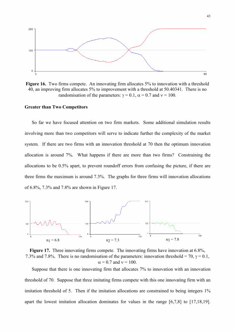
Figure 16. Two firms compete. An innovating firm allocates 5% to innovation with a threshold 40, an improving firm allocates 5% to improvement with a threshold at 50.40341. There is no
randomisation of the parameters: � = 0.1, � = 0.7 and � = 100.
Greater than Two Competitors
So far we have focused attention on two firm markets. Some additional simulation results
involving more than two competitors will serve to indicate further the complexity of the market
system. If there are two firms with an innovation threshold at 70 then the optimum innovation
allocation is around 7%. What happens if there are more than two firms? Constraining the
allocations to be 0.5% apart, to prevent roundoff errors from confusing the picture, if there are
three firms the maximum is around 7.3%. The graphs for three firms will innovation allocations
of 6.8%, 7.3% and 7.8% are shown in Figure 17.
n1 = 6.8 n2 = 7.3 n3 = 7.8
Figure 17. Three innovating firms compete. The innovating firms have innovation at 6.8%, 7.3% and 7.8%. There is no randomisation of the parameters: innovation threshold = 70, � = 0.1,
� = 0.7 and � = 100. Suppose that there is one innovating firm that allocates 7% to innovation with an innovation
threshold of 70. Suppose that three imitating firms compete with this one innovating firm with an
imitation threshold of 5. Then if the imitation allocations are constrained to being integers 1%
apart the lowest imitation allocation dominates for values in the range [6,7,8] to [17,18,19].
44
Outside that range the single innovator dominates. So it appears that for imitators the winning
strategy is to allocate less than competing imitators to imitation. The graphs for the three
imitating firms with an allocation of 11%, 12% and 13% are shown in Figure 18.
m1 = 6.8 m2 = 7.3 m3 = 7.8
Figure 18. Three imitating firms compete with one innovating firm. The innovating firm allocate 7% to innovation with a threshold of 70.. The imitating firms allocate 11%, 12% and
13% with an imitation threshold of 5, � = 0.1, � = 0.7 and � = 100.
Suppose that there are four firms who are prepared to allocate 12% to other than workers and
that:
• the first allocates 6% to imitation and 6% to process improvement
• the second allocates 6% to innovation and 6% to process improvement
• the third allocates 6% to innovation and 6% to imitation
• the fourth allocates 4% to each of innovation, imitation and process improvement
There is no randomisation of the parameters: innovation threshold = 80, imitation threshold = 12,
improvement threshold = 85, � = 0.1, � = 0.7 and � = 100. The sizes of the four firms are shown
in Figure 19. That Figure also shows what happens if the innovation threshold = 84, imitation
threshold = 13, improvement threshold = 90. In both examples the fourth firm with the mixed
strategy across innovation, imitation and improvement performs the worst. Once again the
detailed explanation and understanding of this result is not clear.
45
Firm 1
Firm 2 Firm 3
Firm 4
Figure 23. Size of four firms when: the first allocates 6% to imitation and 6% to process improvement, the second allocates 6% to innovation and 6% to process improvement, the third
allocates 6% to innovation and 6% to imitation, and the fourth allocates 4% to each of innovation, imitation and process improvement. There is no randomisation of the parameters:
innovation threshold = 80, imitation threshold = 12, improvement threshold = 85, � = 0.1, � = 0.7 and � = 100. The second row shows what happens if the innovation threshold = 84, imitation
threshold = 13, improvement threshold = 90.
Conclusion
Our paper shows how the choice of exploration versus exploitation strategies is a complex
problem without any analytical solutions in the form of optimal strategies for individual firms.
This arises in part because innovation, imitation and process improvement are not deterministic
processes and because of interactions among the strategies of different firms. This makes the
whole market system a highly non-linear one. As a result we have to utilise simulation models to
examine the conditions under which different strategies are successful or not in terms of firm and
competitor survival and ROI.
We have show how survival depends on the timing of innovation, imitation and process
improvement and the speed of diffusion and level of penetration of products. These factors affect
the trade-off between the more shorter term gains from exploiting existing or recently developed
new products against the more distant gains from developing new products. Optimal rates of
46
allocating resources have been detected under different threshold and market demand conditions
in markets with two firms competing and these appear to dominate any imitation strategies. We
have also found conditions under which different strategies can co-exist, such as when an imitator
can live off an innovator firm and when a process improver can live with an innovator. Finally
we have begun to examine results for competition among more than two firms.
Much remains to be done in utilizing and extending the model and we have made it available
on the Internet for other researchers to use, as detailed in the appendix. Further simulation
experiments are required to further develop our understanding of the dynamics of competition
and the trade-off between exploration and exploitation strategies under different conditions. So
far our model has fixed strategies for each firm for the duration of the simulation. A next step
would be to build in response functions whereby firms modify the amount of resources they
devote to exploration and exploitation strategies. The challenge is also to undertake studies of the
evolution of existing markets to see the extent to which the model can replicate know patterns of
development and to allow the model to be calibrated against real market parameter values in
particular industries.
Appendix: Model Implementation on the Internet
The “economy” described above has been implemented as a Java applet and is available on the
The use of Microsoft Internet Explorer with Java enabled is recommended.
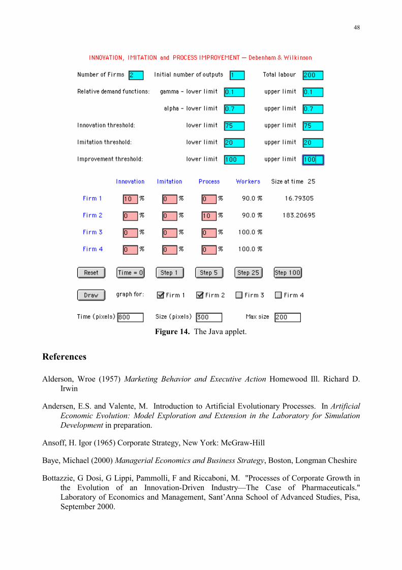
The applet window is in three parts—see Figure 14:
• a “blue boxes” in the top section in which the basic parameters are set.
• a “pink boxes” in the middle in which each firm’s labour is assigned.
• a “white boxes” at the bottom that controls the graphical presentation.
47
The general idea is that the blue boxes in the top half of the applet should be set before the system
is run and may not be changed without initialising the system—ie: by setting time back to zero.
On the other hand the values in the pink boxes may be changed during a run—this enables a
firm’s labour deployment strategy to be modified as things progress. When a run commences, all
of the firms in the simulation produce the same number of products that are unique to each firm.
This initial number of products is set in the top row. The specification of �, �, innovation
threshold, imitation threshold and improvement threshold are given as ranges. If, for example,
the range for � is set to [0.1, 0.1] then � = 0.1. If the range is set to [0.1, 0.2] then � will be set to a
random number in this range. The random distribution used is a truncated normal distribution—
that is, quantities more than 2 standard deviations from the mean are discarded. The left-hand
button “Reset” sets the values in the pink boxes to zero. The “Time = 0” button should be used to
initialise the system before a run. The four buttons “Step 1”,.., “Step 100” move time forward by
the designated amount and the resulting sizes of the firms should appear on the lower right-side
of the applet window. Once the program has been run, the “Draw” button should open another
window with a graph of the resulting firm sizes. The three “white” text boxes at the bottom of
the applet window may be used to control the size and proportions of the graphical output.
48
Figure 14. The Java applet.
References
Alderson, Wroe (1957) Marketing Behavior and Executive Action Homewood Ill. Richard D. Irwin
Andersen, E.S. and Valente, M. Introduction to Artificial Evolutionary Processes. In Artificial Economic Evolution: Model Exploration and Extension in the Laboratory for Simulation Development in preparation.
Ansoff, H. Igor (1965) Corporate Strategy, New York: McGraw-Hill
Baye, Michael (2000) Managerial Economics and Business Strategy, Boston, Longman Cheshire
Bottazzie, G Dosi, G Lippi, Pammolli, F and Riccaboni, M. "Processes of Corporate Growth in the Evolution of an Innovation-Driven Industry—The Case of Pharmaceuticals." Laboratory of Economics and Management, Sant’Anna School of Advanced Studies, Pisa, September 2000.
49
Brown, S., & Eisenhardt, K. M. (1997) ”The art of continuous change:Linking complexity theory and time-paced evolution in relentlesslyshifting organizations” Administrative Science Quarterly,42 (1), 1-34
Bonibeau, Eric and Meyer, Chris (2001) "Swarm Intelligence: A Whole new way of thinking about business" Harvard Business Review (May)
Bonibeau, Eric, Dirigo, Marco and Theraulaz, Guy (1999) Swarm Intelligence: From Natural to Artificial Systems, New York: Oxford University Press
[Cantner, et al, 2000] Cantner, U, Hanusch, H. & Klepper, S. (Eds). Economic Evolution, Learning, and Complexity. Physica Verlag, 2000.
Casti, John L.: Would-Be Worlds: How Simulation is Changing the Frontiers of Science, John Wiley, New York 1997
Chelariu, Cristian, Johnston, Wesley J. and Young, Louise C.(2002) “Learning To Improvise, Improvising To Learn: A Process Of Responding To Complex Environments” Journal of Business Research 55 (February)
Creedy, J and Duncan, D (2002) Behavioural Microsimulation with Labour Supply Responses. Journal of Economic Surveys, 16, 1-39.
Dwyer John (1998) “The Relational View: Cooperative Strategy and Sources of Interorganizational Competitive Advantage” Academy of Management Review, 23: 660-679
Fourt, L.A.and J. W. Woodlock (1960) "Early Prediction of Market Success for New Grocery Products," Journal of Marketing (Oct.) 31-38.
Goldenberg, Jacob, Libai, Barak and Muller, Eitan (2001) "Using Complex Systems Analysis to Advance Marketing Theory Development: Modeling Heterogeneity Effects on New Product Growth through Stochastic Cellular Automata." Academy of Marketing Science Review [Online] 01 (9)
Hamel, Gary and Prahalad, C.K. (1994) Competing for the Future, Cambridge Mass., Harvard University Press.
Hunt, Shelby (2000) A General Theory of Competition Thousand Oaks, Ca. Sage
Iansiti, Marco and Leven, Roy (2002) “The New Operational Dynamics of Business Ecosystems: Implications for Policy, Operations and Technology Strategy” Working Paper 03-030 Harvard Business School
Langton, Chris ed. (1996) Artificial Life: An Overview. Cambridge MA, MIT Press
Lilien, Gary L, Kotler, Philip and K Sridhar Moorthy (1995) Marketing Models Englewood Cliffs NJ; Prentice Hall
50
Mahajan Vijay, Eitan Muller, and Frank M. Bass. 1990. "New Product Diffusion Models in Marketing: A Review and Directions for Research." Journal of Marketing 54 (January): 1-26
March, James G.: Exploration and Exploitation in Organizational Learning. Organizational Science, 2 (February 1991): 71-87.
May, Robert M. (1976) "Simple mathematical models with very complicated dynamics," Nature 261 (June 10), 459-467
Mazzucato, M. Firm Size, Innovation and Market Sructure: The Evolution of Industry Concentration and Instability. Elgar, 2000.
Midgley, D.F., Marks R.E. and Cooper L.G. (1997) "Breeding Competitive Strategies" Management Science, 43 (March) 257-275
Moore, James (1996) The Death of Competition, John Wiley, Chichester.
Moorman, Christine and Miner Anne S.: “The Convergence of Planning and Execu tion: Improvisation in New Product Development.” Journal of Marketing 62 (July 1998a): 1-20.
Moorman, Christine and Miner, Anne S.: “Organizational Improvisation and Organizational Memory.” Academy of Management Review 23 (October 1998b): 698-723.
Nelson, R.R and Winter, S.G. (1982) An Evolutionary Theory of Economic Change. Harvard UP,.
Porter, Michael (1985) Competitive Advantage New York The Free Press
Ruth, M and Hannon, B. (1997) Modelling Dynamic Economic Systems. Springer-Verlag..
Ritter, Thomas. (1999) The Networking Company: Antecedents for Coping With Relationships and Networks Effectively. Industrial Marketing Management 28 (5):467-479
Sowell, Thomas (1972) Say's Law, An Historical Analysis, Princeton University Press
Tesfatsion, Leigh: (1997) How Economists Can Get Alife, in The Economy as an Evolving Complex System II, Arthur, W.B., Durlauf, S. and Lane, D. A. eds., Addison-Wesley Publishing, Redwood City, CA. 1997 pp. 534-564
Tesfatsion, Leigh (2002) Agent-Based Computational Economics: Growing Economies from the Bottom Up. Department of Economics, Iowa State University, Ames, Iowa. ISU Economics Working Paper No. 1. 15 March
Wilkinson, Ian F., Wiley, James B. and Lin, Aizhong (2001) Modelling the Structural Dynamics of Industrial Networks. Interjournal of Complex Systems, Article #409 2001 www.interjournal.org
Hibbert, D. Bryn and Wilkinson, Ian F.(1994) "Chaos in the dynamics of markets" Journal of the Academy of Marketing Science 22:3, 218-233
51
Wilkinson, Ian F., and L. Young (2002) “On Cooperating: Firms, Relations and Networks” Journal of Business Research 55 (February), 123-132
Yildizoglu M, 2002. Modeling Adaptive Learning: R&D Strategies in the Model of Nelson & Winter (1982). Working Papers of E3i..