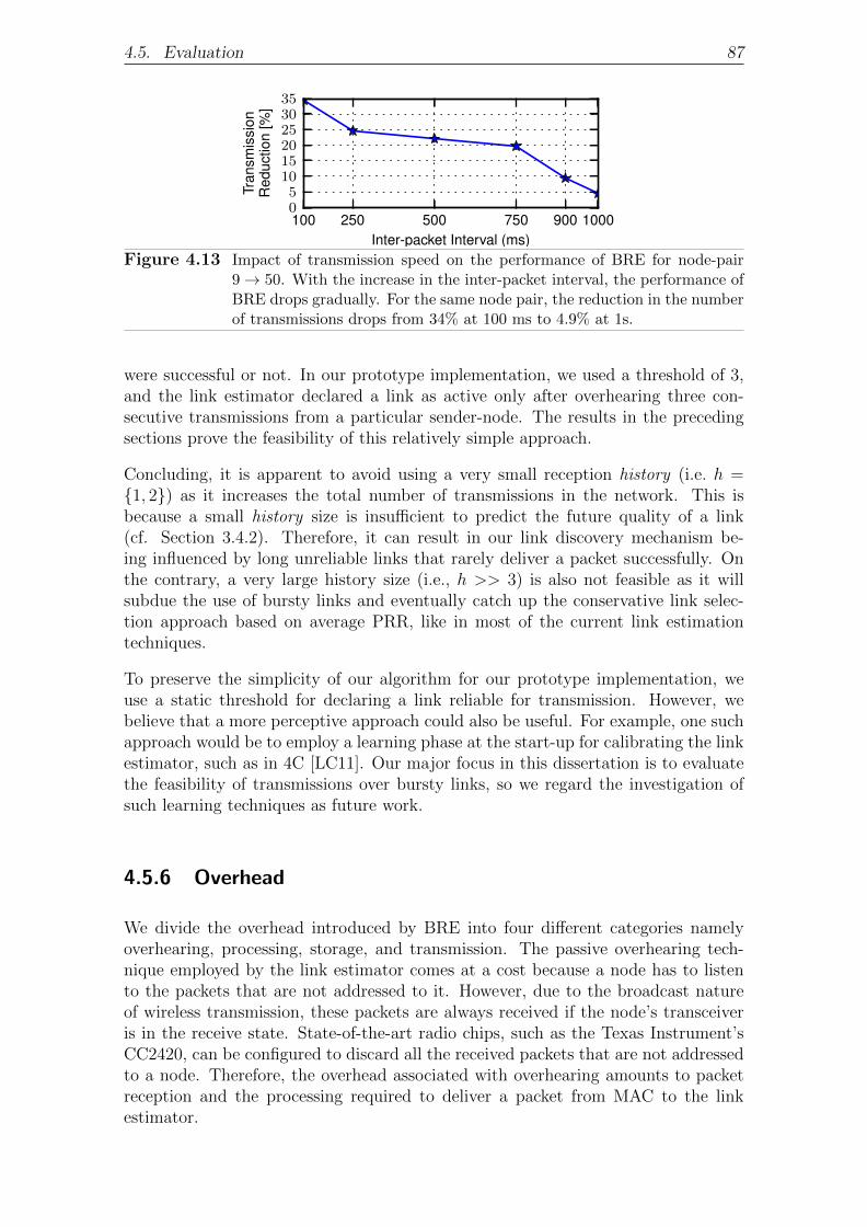
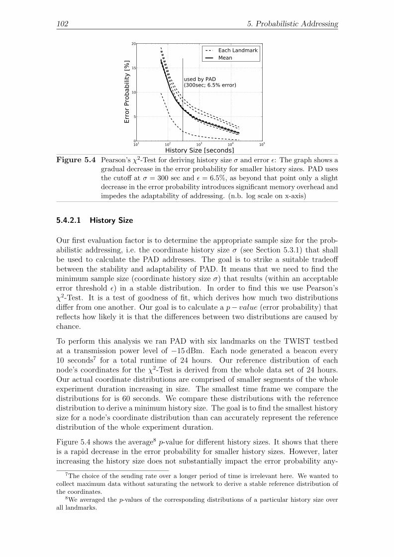
Exploiting Wireless Link Dynamics

Exploiting Wireless Link Dynamics

Von der Fakultat fur Mathematik, Informatik und Naturwissenschaftender RWTH Aachen University zur Erlangung des akademischen Gradeseines Doktors der Ingenieurwissenschaften genehmigte Dissertation

vorgelegt von

M.Sc. Software Systems Engineering

Muhammad Hamad Alizai

aus Haripur

Berichter:

Prof. Dr.-Ing. Klaus WehrleProf. Dr.rer.nat. Bernhard Rumpe

Tag der Mundlichen Prufung 07.03.2012

Diese Dissertation ist auf den Internetseiten der Hochschulbibliothek online verfugbar

I hereby affirm that I composed this work independently and used no other than thespecified sources and tools and that I marked all quotes as such.

Ich erklare hiermit, dass ich die vorliegende Arbeit selbstandig verfasst und keineanderen als die angegebenen Quellen und Hilfsmittel verwendet habe.

Aachen, den 10. Januar 2012

Abstract

Efficient and reliable communication is the key to enable multihop wireless networkssuch as sensornets, meshnets and MANETs. Unlike wired networks, communica-tion links in wireless networks are highly dynamic and pose additional challenges.Network protocols, besides establishing routing paths between two nodes, must over-come link dynamics and the resulting shift in the network topology. Hence, we needto develop efficient link estimation mechanisms, reliable routing algorithms, and sta-ble addressing schemes to overcome these challenges inherent in wireless networks.

The prevalent approach today is to use routing techniques similar to those in wirednetworks, such as tree construction: Link estimators identify neighbors with consis-tently high quality links based on a certain cost metric. Routing protocols conserverouting to a single path between two communication nodes by choosing the best se-quence of nodes at each hop, as identified by the link estimator. In contrast, recentstudies on opportunistic routing schemes suggest that traditional routing may notbe the best approach in wireless networks because it leaves out a potentially largeset of neighbors with intermediate links offering significant routing progress. Fine-grained analysis of link qualities reveals that such intermediate links are bursty, i.e.,alternate between reliable and unreliable periods of transmission.

We propose unconventional yet efficient approaches of link estimation, routing andaddressing in multihop wireless networks to exploit wireless link dynamics insteadof bypassing them for the sake of stability and reliability. The goal is to maximizerouting performance parameters, such as transmission counts and throughput, byexploiting the burstiness of wireless links while, at the same time, preserving thestability and reliability of the existing mechanisms.

The contributions of this dissertation are manifold: Firstly, we develop relevant linkestimation metrics to estimate link burstiness and identify intermediate links thatcan enhance the routing progress of a packet at each hop. Secondly, we proposeadaptive routing extensions that enables the inclusion of such long-range intermedi-ate links into the routing process. Thirdly, we devise a resilient addressing schemeto assign stable locations to nodes in challenging network conditions. Finally, wedevelop an evaluation platform that allows us to evaluate our prototypes across dif-ferent classes of wireless networks, such as sensornets and meshnets, using a singleimplementation.

The dissertation primarily focuses on the network layer of the protocol stack. Al-though the proposed approaches have a broader relevance in the wireless domain, thedesign choices for our prototypes are tailored to sensornets – a notoriously difficultclass of multihop wireless networks. Our evaluation highlights the key achievementsof this work when compared to the state-of-the-art: The proposed metrics identifybursty links in the network with high accuracy, the routing extensions reduce thetransmission count in the network by up to 40%, and the addressing scheme achieves3-7 times more stable addressing even under challenging network conditions.

Zusammenfassung

Effiziente und verlassliche Kommunikation ist der Schlussel, um Multihopkommu-nikation wie sensornets, meshnets und MANETs zu ermoglichen. Im Gegensatzzu kabelgebundenen Netzwerken sind die Kommunikationsverbindungen in kabel-losen Netzen hochdynamisch und stellen weitere Herausforderungen dar. Netzw-erkprotokolle mussen, neben der Vermittlung von Ende-zu-Ende Pfaden, auf dieseVerbin-dungsvariabilitat und die sich daraus ergebenden Anderungen der Netzw-erktopologie reagieren. Folglich besteht ein Bedarf an effizienten Mechanismen zurSchatzung von Verbindungsparametern, verlasslichen Routingmechanismen und sta-bilen Adressier-ungsschemata, um diese inharenten Herausforderungen kabelloserNetzwerke anzugehen.

Heutige Ansatze verwenden ahnliche Techniken wie kabelgebundene Netzwerke, zumBeispiel die Konstruktion von Baumen: Verbindungsschatzer identifizieren Nach-barn, die nach einer vorgegebenen Metrik eine konsistent hohe Qualitat zeigen.Routingprotokolle beschranken sich bei der Wahl einer Route auf einen einzelnenPfad zwischen zwei Kommunikationsknoten, in dem sie bei jedem Schritt den nachdem Verbindungsschatzer besten Knoten wahlen. Im Gegensatz dazu legen aktuelleStudien opportunistischer Routingschemata nahe, dass traditionelle Routingmech-anismen suboptimal arbeiten, da sie Verbindungen mittlerer Qualitat, die einendeutlich großeren Pfadfortschritt ermoglichen wurden, aussparen. Eine genauereUntersuchung der Verbindungsparameter zeigt, dass diese Verbindungen mittlererQualitat schubhaft sind, das heißt, dass sich Perioden verlasslicher mit Periodenunzuverlassiger Ubertragung abwechseln.

In dieser Arbeit werden unkonventionelle aber effiziente Ansatze zur Verbindungss-chatzung, zum Routing und zur Adressierung in Multihop-Netzwerken vorgeschla-gen, die diese Dynamik in kabellosen Netzwerken fur sich nutzen, anstatt sie zumWohle von Pfadstabilitat und Verlasslichkeit einzelner Verbindungen zu ignorieren.Das Ziel ist, Routingperformanzmetriken wie die Zahl der Ubertragungen und denDurchsatz zu maximieren, indem man die Schubhaftigkeit kabelloser Verbindungenausnutzt, wahrend man gleichzeitig die Stabilitat und Verlasslichkeit existierenderAnsatze erhalt.

Dieser Arbeit schlagt folgende Erweiterungen und Verbesserungen vor: Erstens wirdeine Verbindungsmetrik entwickelt, mit Hilfe derer sich die Schubhaftigkeit vonVerbindungen schatzen lasst und diejenigen identifiziert werden konnen, welche beijedem Schritt den Pfadfortschritt verbessern konnen. Zweitens wird eine adaptiveRoutingerweiterung vorgeschlagen, die eine Miteinbeziehung dieser weitreichendenaber nur schubhaft zur Verfugung stehenden Verbindungen in bestehene Routing-mechanismen ermoglicht. Drittens wird ein robustes Adressierungsschema vorgestellt,um Knoten unter dynamischen Netzwerkbedingungen stabile Adressen zuweisen zukonnen. Zuletzt wurde eine Evaluierungsplattform entwickelt, die es erlaubt, Pro-totypen uber verschiedene Klassen von kabellosen Netzwerken, wie sensornets undmeshnets, hinweg mit einer einzigen Implementierung zu untersuchen.

Der Fokus dieser Arbeit liegt primar auf der Netzwerkschicht des Protokollstapels.Obgleich die vorgeschlagenen Ansatze eine breitere Relevanz in kabellosen Netzw-erken haben, orientieren sich die Designentscheidungen an sensornets, welche fur ihrestringenten Herausforderungen bekannt sind. Unsere Evaluation hebt ein Schlussel-

ergebnis beim Vergleich dieser Arbeit mit dem aktuellen Stand der Technik heraus:Die vorgeschlagenen Metriken identifizieren schubhaft verfugbare Verbindungen mithoher Genauigkeit, die Routingerweiterungen reduzieren die Zahl der Ubertragun-gen um 40%, und das Adressierungsschema erreicht eine um 3 bis 7-fach stabilereAdressierung selbst unter schwierigen und dynamischen Netzwerkbedingungen.

Acknowledgments

Who else to thank first but Allah, the most merciful and benevolent

I owe a lot to Professor Klaus Wehrle for keeping trust in me and making me believeas if I am one of his special students. Feeling special brings a lot of pressure aswell because I always thought one day he will definitely get to know that I am notas intelligent and smart as he thinks. I am glad (or at least hope that) this daynever came throughout my stay at ComSys. He hired me as a raw student andtransformed me into a self-confident scientist who is willing to take on the strongestof the research challenges in his field. Thank you Klaus for everything that you didfor me during my tenure both as a master and as a PhD student at ComSys. Iwill never forget that you prepared my IPSN 2010 poster on PAD. I am honored tohave Professor Bernhard Rumpe as my 2nd PhD advisor and thankful to him forhis highly valuable feedback, support, and prompt responses to my urgent requests.

Many thanks to my dearest ComSys colleagues (sorry guys, as much as I wouldloved to, I cannot mention your names because ComSys team has recently grownexponentially) for having to deal with my minimal German language skills, for in-teresting discussions and research colloquiums, for giving feedback on my talks andresearch papers, and of course for anything that I don’t remember as of now. Mycoauthors Olaf, Jo, Hanno, Raimondas, Georg, Tobias V., Stefan, and Klaus mademy papers look much better. Jo is one of the most amazing person I have ever met.I must thank him and Ismet for all the fun that we had together and I am sure thatI will never be able to find roommates like them.

I am also highly indebted to ComSys thesis students Alexander, Tobias V., Ben-jamin, Bernhard and Andrea for their magnificent input in this dissertation work.These acknowledgements will be incomplete without thanking the technical and sec-retarial staff at ComSys because they helped me big time with all the administrativetasks.

Last but not the least, the never ending support and love since childhood and prayersof my parents are the reasons I am able to write this dissertation. I am thankful tomy wife, for her continuous support and for being patient in tough days especiallycloser to paper submission deadline. How can I forget to thank my two year old sonAbdul Ahad for his special treatment of my laptop (the only undamaged belongingat my home) and reminding me time and again that life is not all about doingresearch and writing papers.

Contents

1 Introduction 1

1.1 Problem Statement . . . . . . . . . . . . . . . . . . . . . . . . . . . . 2

1.2 Observations . . . . . . . . . . . . . . . . . . . . . . . . . . . . . . . . 3

1.3 Major Contributions . . . . . . . . . . . . . . . . . . . . . . . . . . . 3

1.3.1 Link Estimation . . . . . . . . . . . . . . . . . . . . . . . . . . 4

1.3.2 Routing . . . . . . . . . . . . . . . . . . . . . . . . . . . . . . 5

1.3.3 Addressing . . . . . . . . . . . . . . . . . . . . . . . . . . . . . 5

1.3.4 Wi-Fi Evaluation . . . . . . . . . . . . . . . . . . . . . . . . . 5

1.4 Limitations . . . . . . . . . . . . . . . . . . . . . . . . . . . . . . . . 5

1.5 Target Environments . . . . . . . . . . . . . . . . . . . . . . . . . . . 6

1.6 Structure . . . . . . . . . . . . . . . . . . . . . . . . . . . . . . . . . 6

2 Multihop Wireless Routing: Qualitative Perspective 9

2.1 Link Estimation . . . . . . . . . . . . . . . . . . . . . . . . . . . . . . 10

2.1.1 Introduction . . . . . . . . . . . . . . . . . . . . . . . . . . . . 10

2.1.1.1 Table Management . . . . . . . . . . . . . . . . . . . 11

2.1.1.2 Key Properties . . . . . . . . . . . . . . . . . . . . . 12

2.1.2 Case Studies . . . . . . . . . . . . . . . . . . . . . . . . . . . . 12

2.1.2.1 Four-Bit Link Estimation . . . . . . . . . . . . . . . 13

2.1.2.2 Solicitation based Forwarding . . . . . . . . . . . . . 15

2.1.3 Qualitative Comparison with BLE . . . . . . . . . . . . . . . 17

2.2 Routing . . . . . . . . . . . . . . . . . . . . . . . . . . . . . . . . . . 18

2.2.1 Introduction . . . . . . . . . . . . . . . . . . . . . . . . . . . . 19

2.2.1.1 Tree Construction . . . . . . . . . . . . . . . . . . . 20

2.2.1.2 Key Properties . . . . . . . . . . . . . . . . . . . . . 21

2.2.2 Case Studies . . . . . . . . . . . . . . . . . . . . . . . . . . . . 22

2.2.2.1 Collection Tree Protocol . . . . . . . . . . . . . . . . 22

2.2.2.2 Opportunistic Routing . . . . . . . . . . . . . . . . 24

2.2.2.3 AODV . . . . . . . . . . . . . . . . . . . . . . . . . . 26

2.2.3 Qualitative Comparison with BRE . . . . . . . . . . . . . . . 28

2.3 Addressing . . . . . . . . . . . . . . . . . . . . . . . . . . . . . . . . . 29

2.3.1 Introduction . . . . . . . . . . . . . . . . . . . . . . . . . . . . 29

2.3.1.1 Challenges . . . . . . . . . . . . . . . . . . . . . . . 29

2.3.1.2 Key Properties . . . . . . . . . . . . . . . . . . . . . 30

2.3.2 Case Studies . . . . . . . . . . . . . . . . . . . . . . . . . . . . 30

2.3.2.1 Beacon Vector Routing (BVR) . . . . . . . . . . . . 31

2.3.2.2 Small State and Small Routing (S4) . . . . . . . . . 32

2.3.3 Qualitative Comparison with PAD . . . . . . . . . . . . . . . 34

2.4 Summary . . . . . . . . . . . . . . . . . . . . . . . . . . . . . . . . . 36

3 Estimating Link Burstiness 39

3.1 Motivation . . . . . . . . . . . . . . . . . . . . . . . . . . . . . . . . . 40

3.1.1 Link Categorization . . . . . . . . . . . . . . . . . . . . . . . . 40

3.1.2 Requirements . . . . . . . . . . . . . . . . . . . . . . . . . . . 41

3.1.3 Major Contributions . . . . . . . . . . . . . . . . . . . . . . . 42

3.2 Related Work . . . . . . . . . . . . . . . . . . . . . . . . . . . . . . . 42

3.2.1 Measuring Link Burstiness . . . . . . . . . . . . . . . . . . . . 42

3.2.2 Short Term Link Estimation (STLE) . . . . . . . . . . . . . . 43

3.2.3 Long Term Link Estimation (LTLE) . . . . . . . . . . . . . . 43

3.2.4 Estimating Multiple Link Properties . . . . . . . . . . . . . . 43

3.3 Problem Analysis . . . . . . . . . . . . . . . . . . . . . . . . . . . . . 44

3.3.1 The Need to Utilize Bursty Links . . . . . . . . . . . . . . . . 45

3.3.2 Basic Concept . . . . . . . . . . . . . . . . . . . . . . . . . . . 46

3.3.3 Design Goals . . . . . . . . . . . . . . . . . . . . . . . . . . . 47

3.4 Deriving Metrics for Bursty Links . . . . . . . . . . . . . . . . . . . . 48

3.4.1 Data Set and Experimental Model . . . . . . . . . . . . . . . 48

3.4.2 Predicting Transmission Success from a Short History . . . . . 49

3.4.3 Online Estimation of Link Burstiness . . . . . . . . . . . . . . 51

3.4.3.1 MAC3 . . . . . . . . . . . . . . . . . . . . . . . . . . 52

3.4.3.2 Example . . . . . . . . . . . . . . . . . . . . . . . . . 52

3.4.3.3 Results . . . . . . . . . . . . . . . . . . . . . . . . . 53

3.4.4 Estimating Burst Lengths . . . . . . . . . . . . . . . . . . . . 54

3.4.4.1 EFT . . . . . . . . . . . . . . . . . . . . . . . . . . . 55

3.4.4.2 Example . . . . . . . . . . . . . . . . . . . . . . . . . 55

3.4.4.3 Results . . . . . . . . . . . . . . . . . . . . . . . . . 56

3.5 The Bursty Link Estimator . . . . . . . . . . . . . . . . . . . . . . . 56

3.5.1 Link Quality Metric . . . . . . . . . . . . . . . . . . . . . . . 56

3.5.2 Table Management . . . . . . . . . . . . . . . . . . . . . . . . 58

3.5.3 Evaluation . . . . . . . . . . . . . . . . . . . . . . . . . . . . . 59

3.5.3.1 Link History Size . . . . . . . . . . . . . . . . . . . . 59

3.5.3.2 Link Estimation . . . . . . . . . . . . . . . . . . . . 59

3.5.3.3 Routing . . . . . . . . . . . . . . . . . . . . . . . . . 60

3.6 Summary . . . . . . . . . . . . . . . . . . . . . . . . . . . . . . . . . 62

4 Routing over Bursty Wireless Links 63

4.1 Introduction . . . . . . . . . . . . . . . . . . . . . . . . . . . . . . . . 64

4.1.1 Significance . . . . . . . . . . . . . . . . . . . . . . . . . . . . 64

4.1.2 Key Features . . . . . . . . . . . . . . . . . . . . . . . . . . . 64

4.2 Related Work . . . . . . . . . . . . . . . . . . . . . . . . . . . . . . . 65

4.2.1 4C: Wireless Link Prediction . . . . . . . . . . . . . . . . . . . 66

4.2.2 ExOR: Opportunistic Routing . . . . . . . . . . . . . . . . . . 66

4.2.3 Backpressure Collection Protocol (BCP) . . . . . . . . . . . . 67

4.3 System Overview . . . . . . . . . . . . . . . . . . . . . . . . . . . . . 67

4.3.1 Basic Concept . . . . . . . . . . . . . . . . . . . . . . . . . . . 68

4.3.2 Design Goals . . . . . . . . . . . . . . . . . . . . . . . . . . . 68

4.4 Bursty Routing Extensions . . . . . . . . . . . . . . . . . . . . . . . . 69

4.4.1 Algorithm . . . . . . . . . . . . . . . . . . . . . . . . . . . . . 69

4.4.1.1 Link Discovery . . . . . . . . . . . . . . . . . . . . . 70

4.4.1.2 Link Announcement . . . . . . . . . . . . . . . . . . 70

4.4.1.3 Routing Mode . . . . . . . . . . . . . . . . . . . . . 71

4.4.1.4 Link Unavailability . . . . . . . . . . . . . . . . . . . 71

4.4.2 Integration with Routing Protocols . . . . . . . . . . . . . . . 71

4.4.3 Design Challenges . . . . . . . . . . . . . . . . . . . . . . . . . 73

4.4.3.1 Reliability . . . . . . . . . . . . . . . . . . . . . . . . 73

4.4.3.2 Stability and Adaptability . . . . . . . . . . . . . . . 73

4.4.3.3 Loops . . . . . . . . . . . . . . . . . . . . . . . . . . 74

4.4.4 Duplicate Transmissions . . . . . . . . . . . . . . . . . . . . . 74

4.5 Evaluation . . . . . . . . . . . . . . . . . . . . . . . . . . . . . . . . . 75

4.5.1 Implementation . . . . . . . . . . . . . . . . . . . . . . . . . . 75

4.5.2 Experimental Setup . . . . . . . . . . . . . . . . . . . . . . . . 76

4.5.3 Performance . . . . . . . . . . . . . . . . . . . . . . . . . . . . 76

4.5.3.1 Transmission Cost . . . . . . . . . . . . . . . . . . . 79

4.5.3.2 Reliability . . . . . . . . . . . . . . . . . . . . . . . . 80

4.5.3.3 Throughput . . . . . . . . . . . . . . . . . . . . . . . 81

4.5.3.4 Comparison with Strawman . . . . . . . . . . . . . . 82

4.5.3.5 Node Density and State Maintenance . . . . . . . . . 83

4.5.4 Intermediate Link Characteristics . . . . . . . . . . . . . . . . 83

4.5.4.1 Transmissions Cost vs. Intermediate Links . . . . . . 84

4.5.4.2 Timeliness . . . . . . . . . . . . . . . . . . . . . . . . 85

4.5.4.3 Inter-packet Intervals . . . . . . . . . . . . . . . . . . 85

4.5.5 A Sanity Check for BLE Thresholds . . . . . . . . . . . . . . 86

4.5.6 Overhead . . . . . . . . . . . . . . . . . . . . . . . . . . . . . 87

4.6 Summary . . . . . . . . . . . . . . . . . . . . . . . . . . . . . . . . . 88

5 Probabilistic Addressing 91

5.1 Motivation . . . . . . . . . . . . . . . . . . . . . . . . . . . . . . . . . 92

5.1.1 Approach . . . . . . . . . . . . . . . . . . . . . . . . . . . . . 92

5.1.2 Major Contributions . . . . . . . . . . . . . . . . . . . . . . . 93

5.2 Preliminaries . . . . . . . . . . . . . . . . . . . . . . . . . . . . . . . 93

5.2.1 Basic Idea . . . . . . . . . . . . . . . . . . . . . . . . . . . . . 94

5.2.2 Target Networks . . . . . . . . . . . . . . . . . . . . . . . . . 95

5.2.2.1 Sensornets . . . . . . . . . . . . . . . . . . . . . . . . 95

5.2.2.2 Manets and Meshnets . . . . . . . . . . . . . . . . . 96

5.3 Probabilistic Addressing Explained . . . . . . . . . . . . . . . . . . . 96

5.3.1 Coordinate History . . . . . . . . . . . . . . . . . . . . . . . . 96

5.3.2 Address Calculation . . . . . . . . . . . . . . . . . . . . . . . 97

5.3.3 Address Dissemination . . . . . . . . . . . . . . . . . . . . . . 98

5.3.3.1 Hidden Loop Avoidance . . . . . . . . . . . . . . . . 99

5.3.4 Summary . . . . . . . . . . . . . . . . . . . . . . . . . . . . . 99

5.4 Performance Evaluation of PAD . . . . . . . . . . . . . . . . . . . . . 100

5.4.1 Testbeds and Experimental Setup . . . . . . . . . . . . . . . . 100

5.4.2 Determining the System Parameters . . . . . . . . . . . . . . 101

5.4.2.1 History Size . . . . . . . . . . . . . . . . . . . . . . . 102

5.4.2.2 Error Threshold . . . . . . . . . . . . . . . . . . . . 103

5.4.3 Comparison with BVR and S4 . . . . . . . . . . . . . . . . . . 103

5.4.3.1 Address Stability . . . . . . . . . . . . . . . . . . . . 105

5.4.3.2 Address Monotony: Magnitude of Change . . . . . . 105

5.4.3.3 Hop Distance . . . . . . . . . . . . . . . . . . . . . . 107

5.4.3.4 Node Dynamics . . . . . . . . . . . . . . . . . . . . . 107

5.4.3.5 Summary and Comparison with CTP . . . . . . . . . 109

5.5 Routing on PAD . . . . . . . . . . . . . . . . . . . . . . . . . . . . . 110

5.5.1 Address Prediction . . . . . . . . . . . . . . . . . . . . . . . . 111

5.5.2 Distance Function . . . . . . . . . . . . . . . . . . . . . . . . . 111

5.5.2.1 Minimize Distance . . . . . . . . . . . . . . . . . . . 111

5.5.2.2 Link Age . . . . . . . . . . . . . . . . . . . . . . . . 112

5.5.2.3 Link Asymmetry . . . . . . . . . . . . . . . . . . . . 113

5.6 Routing Results . . . . . . . . . . . . . . . . . . . . . . . . . . . . . . 113

5.6.1 Experimental Setup . . . . . . . . . . . . . . . . . . . . . . . . 114

5.6.2 Number of Transmissions . . . . . . . . . . . . . . . . . . . . . 114

5.6.3 Reliability . . . . . . . . . . . . . . . . . . . . . . . . . . . . . 116

5.6.4 Memory and Communication Overhead . . . . . . . . . . . . . 116

5.7 Discussion and Related Work . . . . . . . . . . . . . . . . . . . . . . 119

5.7.1 Sensornets . . . . . . . . . . . . . . . . . . . . . . . . . . . . . 119

5.7.2 Meshnets . . . . . . . . . . . . . . . . . . . . . . . . . . . . . 120

5.8 Summary . . . . . . . . . . . . . . . . . . . . . . . . . . . . . . . . . 120

6 Exploring General Applicability 123

6.1 TinyWifi . . . . . . . . . . . . . . . . . . . . . . . . . . . . . . . . . . 124

6.1.1 Preliminaries . . . . . . . . . . . . . . . . . . . . . . . . . . . 126

6.1.1.1 TinyOS . . . . . . . . . . . . . . . . . . . . . . . . . 126

6.1.1.2 Design Overview . . . . . . . . . . . . . . . . . . . . 128

6.1.1.3 Key Features . . . . . . . . . . . . . . . . . . . . . . 128

6.1.2 Detailed Architecture . . . . . . . . . . . . . . . . . . . . . . . 129

6.1.2.1 Radio Communication . . . . . . . . . . . . . . . . . 129

6.1.2.2 Split-Phase Operation . . . . . . . . . . . . . . . . . 130

6.1.2.3 Timers . . . . . . . . . . . . . . . . . . . . . . . . . . 131

6.1.2.4 Miscellaneous Services . . . . . . . . . . . . . . . . . 132

6.1.3 Evaluating TinyWifi Implementation . . . . . . . . . . . . . . 133

6.1.3.1 Link Layer . . . . . . . . . . . . . . . . . . . . . . . 134

6.1.3.2 Network Layer . . . . . . . . . . . . . . . . . . . . . 134

6.1.4 Limitations . . . . . . . . . . . . . . . . . . . . . . . . . . . . 136

6.1.5 Related Work . . . . . . . . . . . . . . . . . . . . . . . . . . . 137

6.2 Evaluating PAD in IEEE 802.11 . . . . . . . . . . . . . . . . . . . . . 138

6.2.1 Testbed Evaluation . . . . . . . . . . . . . . . . . . . . . . . . 138

6.2.1.1 Address Stability . . . . . . . . . . . . . . . . . . . . 139

6.2.1.2 Hop Distance . . . . . . . . . . . . . . . . . . . . . . 140

6.2.1.3 Routing Cost . . . . . . . . . . . . . . . . . . . . . . 140

6.2.2 Evaluating PAD in Mobility . . . . . . . . . . . . . . . . . . . 141

6.2.2.1 Experimental Setup . . . . . . . . . . . . . . . . . . 141

6.2.2.2 Results . . . . . . . . . . . . . . . . . . . . . . . . . 142

6.3 Summary . . . . . . . . . . . . . . . . . . . . . . . . . . . . . . . . . 144

7 Discussion and Conclusions 145

7.1 Summary . . . . . . . . . . . . . . . . . . . . . . . . . . . . . . . . . 146

7.1.1 Link Estimation . . . . . . . . . . . . . . . . . . . . . . . . . . 146

7.1.2 Routing . . . . . . . . . . . . . . . . . . . . . . . . . . . . . . 147

7.1.3 Addressing . . . . . . . . . . . . . . . . . . . . . . . . . . . . . 148

7.1.4 Portable Protocol Evaluation . . . . . . . . . . . . . . . . . . 148

7.2 Lessons Learnt . . . . . . . . . . . . . . . . . . . . . . . . . . . . . . 149

7.2.1 Intermediate Links are Bursty . . . . . . . . . . . . . . . . . . 149

7.2.2 Bursty Links are Useful for Routing . . . . . . . . . . . . . . . 149

7.2.3 Nodes can be Addressed Probabilistically . . . . . . . . . . . . 149

7.2.4 Network Protocols are Directly Portable . . . . . . . . . . . . 150

7.3 Future Work . . . . . . . . . . . . . . . . . . . . . . . . . . . . . . . . 150

7.3.1 Integrating BLE with Routing Protocols . . . . . . . . . . . . 150

7.3.2 Exploring BRE alternatives . . . . . . . . . . . . . . . . . . . 150

7.3.3 Routing Algorithms for PAD . . . . . . . . . . . . . . . . . . . 151

7.3.4 Evolving TinyWifi . . . . . . . . . . . . . . . . . . . . . . . . 151

Bibliography 153

List of Figures 167

List of Tables 173

Nomenclature 175

Index 177

1Introduction

Wireless links vary significantly in their quality [ABB+04, CWPE05, CWK+05a].Hence, unlike wired networks, the number of packets received by each neighboringnode depends upon the quality of the link between a node and its neighbor. Severalfactors contribute to these variations among link qualities across a wireless network.For example, physical distance between a node and its neighbor [ZG03, BLKW08,ALWB08], environmental conditions [Rap01,PH06], and the interference experiencedby each link from nearby networks operating in the same frequency range [HP09,KHC09,QZW+07,Nic07]. These link variations are well understood at the physicallayer and have led to revolutionary developments in radio access technologies suchas cellular networks.

However, the network protocols that use wireless medium do not understand thesevariations and cannot handle their implications [Sri10]. This is because these pro-tocols are built on top of a link1 abstraction which ignores the spatial and temporalproperties of links. Consequently, network protocols tend to overlook these varia-tions by limiting communications to only high quality and stable links. For example,routing protocols establish a tree based routing infrastructure where each node onlycommunicates with its parent – typically a neighboring node with the best link qual-ity and minimum hop distance to the root. This results in (1) a stable and clear-cutrouting topology, (2) usage of short range links and little routing progress on eachhop, and (3) heavy utilization of the selected links. We believe that this is notthe optimal way to achieve multihop routing in a wireless network as it potentiallyignores very useful links.

Previous studies [ABB+04, SKAL08, ZZHZ10] have shown that links follow certainpatterns in their quality variations, especially the links with intermediate quality.For example, links show correlation in packet reception over time, i.e., they arebursty. We believe that by exploiting the underlying patterns of link variations,we can enable better utilization of links from routing perspective. This dissertation

1For simplicity, we use the term link as an abbreviation for wireless link throughout this dis-sertation

2 1. Introduction

thus tries to explore these patterns, express them in the form of a protocol metric,and exploit them by developing relevant protocol extensions.

1.1 Problem Statement

Achieving multihop communication in a wireless network deals with three differentmechanisms: (1) link estimation, (2) routing, and (3) addressing.

Link estimation is concerned with identifying high quality links within a node’sone-hop neighborhood. These links are typically identified based on the long-termsuccess rate of a link collected over a time frame in the order of minutes (or evenhours) [BLKW08]. Although, in good network conditions, this approach is useful inmaintaining a stable topology, this long term binding restricts a network in how wellit can adapt to link dynamics. Hence, state-of-the-art link estimators are maladap-tive in their operation. For example, in a sparse network with low density of nodes,a node might have no high-quality neighbor in its communication range, requiring amechanism to deal with unstable connectivity. Similarly, today’s link estimators arepessimistic in their link selection: They prefer short-ranged high-quality links overintermittently connected links that might reach farther into the network. Such linkscould offer better routing progress and hence reduce the number of transmissions,lower energy usage in the network, and increase throughput.

Routing protocols use link estimators to establish routing paths in the network thatspan multiple hops. A straightforward mechanism is to establish a tree-like topol-ogy by selecting the best quality link at each hop that minimizes the remainingdistance (in hops) to the destination. We refer to this approach as traditional rout-ing throughout this dissertation. Similar to link estimation, stability prevails overadaptability in today’s routing protocols [RSBA07a]. It means that maintaining astable routing tree is the ultimate goal of the existing routing algorithms. Hence,they are conservative in their path selection and only achieve suboptimal routingprogress at each hop [RSBA07a,BM05a]. Their design is intentionally unable to re-alize fluctuations in the link qualities over a routing path. This is why they employlink estimators in the first place to identify long term stable links in the network.

Finally, an addressing scheme is required to achieve point to point communicationin a multihop wireless network. A common scheme is to assign virtual coordinatesto nodes: Construct multiple trees rooted at landmarks – designated nodes – anddetermine a node’s location based on the vector of hop counts from a set of land-marks. The main challenge in such tree based addressing and routing schemes isthat the changes at one node induce changes in all child nodes further down the tree.Hence, in unstable conditions, such schemes suffer heavily from rapid topologicalchanges due to varying link conditions in the network. To cope with this challenge,maintaining trees and virtual coordinates across the network which are particularlyconsistent is understandably the main objective of these schemes. Therefore, theywillingly concede performance penalties to achieve this objective.

1.2. Observations 3

1.2 Observations

A key assumption that implicates the basic design philosophy of today’s wirelessnetwork protocols is that packet reception and packet loss events over a link areindependent from each other [Sri10]. This relatively simple assumption has had amajor influence in setting the functional level details of the three different mecha-nisms discussed in the previous section. For example, link estimators express thequality of a link by taking a moving average over a link’s packet reception rates.Hence, no consideration, whatsoever, is given to the correlated packet loss events.This can be detrimental for the network performance if such loss events are relativelylonger and go unnoticed at the routing layer. Similarly, this assumption implies thataddressing and routing protocols cannot predict the fate of future transmissions overa link based on its very recent transmission history. Hence, it compels these proto-cols (1) to employ the naive method, i.e., use the best quality link at each hop, and(2) to avoid quick adaptation to the underlying link conditions as it leads to typicalrouting pathologies such as loops and network partitioning.

Our empirical observations contradict this assumption of independent packet lossesover a link and thereby undermines many of the design decisions of today’s routingprotocols. Table 1.1 presents our key observations that form the basis of the conceptspresented in this dissertation.

1.3 Major Contributions

While negating the underlying assumption of today’s routing infrastructure in wire-less networks, the observations in Table 1.1 lead to an important conclusion: Inter-mediate quality links are useful for enhancing the performance of today’s routingprotocols. However, the utility of such links for routing lies in three key questions:

• Can we define this correlation in packet reception over a link in terms of ametric that can be calculated at runtime?

• Can such a metric be used by routing protocols to include links with correlatedpacket reception (i.e., bursty links) for enhancing performance parameters,such as throughput and number of transmissions, without compromising thestringent stability and reliability requirements of today’s applications?

• Can we formulate an addressing scheme that allows for inclusion of such linksinto the routing infrastructure while assigning stable locations to nodes?

This dissertation provides an affirmative answer to these questions by developingrelevant mechanisms for all the three levels of wireless routing infrastructure. More-over, this dissertation also demonstrates the generality of the presented mechanismsacross multiple classes of wireless networks, such as IEEE 802.11 (Wi-Fi) and IEEE802.15.4 (ZigBee).

4 1. Introduction

Empirical Comparison with Implication onobservation today’s assumptions dissertation concept

More than 60% of theunused links in the net-work offer better routingprogress than the linksused by routing protocols.

Today’s routing protocolonly achieve suboptimalperformance in terms ofpath stretch, i.e., numberof hops enroute to destina-tion.

Using such links couldshorten the path stretchand thereby increasethroughput and reducethe number of transmis-sions.

More than 70% of theseunused links are bursty– alternate between reli-able and unreliable trans-mission periods.

Packet loss events over alink are not necessarily in-dependent.

Such links can be used forpacket forwarding duringtheir reliable transmissionperiods.

The probability of nexttransmission being suc-cessful over a link in-creases with the number ofprevious successful trans-missions.

Protocols can predict,with high probability, thefate of future transmis-sions over a link.

We can possibly identifyreliable transmission peri-ods on a bursty link.

Due to unstable connec-tivity, a node’s distancefrom a landmark vary sig-nificantly over time.

Assigning a static, currentvector of hop counts leadsto unstable addressing.

We need to find a mecha-nism that locates and ad-dresses a node using vari-ability patterns instead ofan absolute vector.

Table 1.1 Key observations and their implications on the concepts presented in this dis-sertation. These observations are based on the empirical data collected fromwidely used wireless testbeds such as MoteLab [WASW05], Indriya [DCA09], Mi-rage [CBA+05], TWIST [HKWW06] and SWAN [Sta].

1.3.1 Link Estimation

The basic concept of our link estimation mechanism is to express the quality of alink in terms of how bursty it is. For this purpose we introduce two link metrics:First, we present MAC3 – Moving Average Conditional packet delivery function –as a lightweight metric that estimates the burstiness of links based on the recentdelivery traces at runtime. MAC3 helps us in separating links that show correlatedpacket reception (i.e., bursty links) from the links that do not. Second, we defineEFT – Expected Future Transmissions – as a metric to estimate the duration forwhich a bursty link remains reliable for transmission. EFT helps us in determiningif the reliable transmission periods over a link are large enough to be used for packetforwarding. We also show that EFT is strongly correlated to MAC3. Both thesemetrics are mandatory to determine whether or not an intermediate link is bene-ficial to the overall routing performance. Finally, based on these two metrics, weintroduce a Bursty Link Estimator (BLE), derive requisite parameters for its usage,and evaluate its efficacy in estimating intermediate links. Our results indicate thatBLE identifies bursty links in the network with high accuracy, hence paving the wayfor such links to be included into the routing infrastructure.

1.4. Limitations 5

1.3.2 Routing

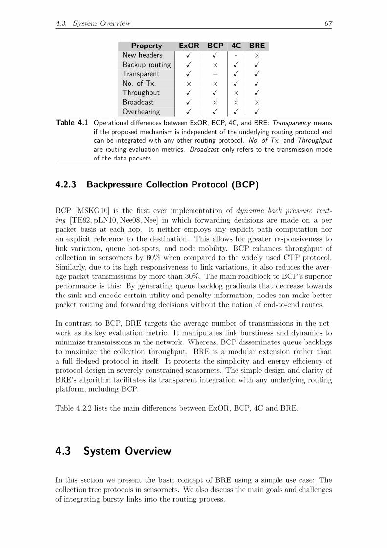
To effectively utilize BLE, we present Bursty Routing Extensions (BRE) that dy-namically selects bursty links during the course of transmission. BRE describes amechanism to implicity changes a node’s parents without disrupting the underlyingrouting topology. Our evaluation on widely used testbeds indicate that BRE achievesan average of 19% and a maximum of 42% reduction in the number of transmissionswhen compared to other state-of-the-art proposals. Moreover, we show that bothBLE and BRE are not tied to any specific routing protocol and integrate seamlesslywith existing routing protocols and link estimators.

1.3.3 Addressing

We present a new addressing scheme, named Probabilistic ADdressing (PAD), thatassigns probabilistic addresses to nodes. In PAD, a node learns from its past loca-tions and calculates the probability distribution over its recent hop distances fromlandmarks. This probability distribution is then used as an address of the node andit incorporates all possible paths leading to landmarks. Hence, a node’s location isdefined in terms of the probability that it exists in a certain location and remainsindependent from the packet loss at shorter time scales. All other nodes in thenetwork predict the current location of a node in its distribution. Our evaluationshows that PAD requires 3-7 times fewer address changes and even a simple routingstrategy over PAD reduces the number of transmissions in the network by 26%.

1.3.4 Wi-Fi Evaluation

Finally, we show that the utility of BLE, BRE and PAD is not limited to any spe-cific class of wireless network. Although our detailed protocol evaluation targetssensornets – a notoriously difficult class of wireless mesh networks – we prove thegenerality of our mechanisms by evaluating them across multiple classes of wirelessnetworks. However, our goal is to avoid tedious re-implementation required to runprotocols in different classes of wireless networks due to the lack of an integrateddevelopment environment. This typically restrict the developers to explore the fea-sibility of their protocols in only one class of wireless network and implicitly assumetheir applicability in the other [AKL+10,AWK+11a].

To this end, we introduce TinyWifi, a platform for executing native sensornets pro-tocols on Linux-driven wireless devices. TinyWifi builds on nesC [GLvB+03a] codebase that abstracts from TinyOS [LMG+04] and enables the execution of nesC-based protocols in Linux. Using TinyWifi as an evaluation and runtime platform,we demonstrate the superior performance of BRE, and PAD in IEEE 802.11 basednetworks as well.

1.4 Limitations

This dissertation also highlights the limitations of the proposed mechanisms. Forexample, BRE assumes dense deployments where a node has many neighbors to

6 1. Introduction

choose from. Higher density of nodes increases the probability of finding a neigh-boring node with bursty link that offers better routing progress. Similarly, packettransmission rates also play a crucial role in determining the performance of BRE.This is because sending packets at higher rates over bursty links maintains a strongcorrelation between their success or failure providence. While by sending packetsfurther apart, this correlation does not hold necessarily [Sri10].

The addressing scheme, i.e., PAD, is highly beneficial in challenging networkingconditions with frequent variations in link qualities. However, it only performs asgood as the state-of-the-art protocols in stable conditions dominated by good links.This is because in stable conditions both the probability distribution and the staticvector of a node’s hop distances from landmarks are almost identical.

We also discuss the memory usage, computational overhead and transmission costof BLE, BRE and PAD. Each of these mechanisms offer a number of design choicesand trade-offs between their efficiency and overhead. For example, PAD results inlarger node addresses but allows to trade-off transmission overhead against memoryoverhead in how address information is disseminated in the network. The first optionis to include a node’s address in broadcast beacons which increases the beacon size.The second option is to only transmit a node’s current hop distance from landmarksinstead of the aggregated distribution. In this case, the neighbors that receive thebeacon need to store a history of theses coordinates and compute the PAD addressthemselves.

1.5 Target Environments

Sensornets and meshnets provide flexible and robust ways of establishing networkstructures without the need for an exhaustive infrastructure. Routing structures inthese networks are self-established and -maintained and depend on the presence ofwireless links between nodes in the network. A resource-efficient utilization of thesestructures greatly increases throughput and network lifetime and reduces transmis-sion energy and failures. Our work thus targets sensornets and meshnets due to theirequivalent routing mechanisms. Although our analysis comprises empirical data fromboth IEEE 802.15.4 and 802.11 based wireless networks, the design choices are tai-lored to sensornets. This is because our prototypes and their evaluation targets thisembedded class of wireless networks.

1.6 Structure

The remainder of this dissertation is structured as follows.

Chapter 2 provides background information by revisiting the fundamentals of linkestimation, routing, and addressing concepts in wireless networks. It presents thestate-of-the-art case studies in these three areas and qualitatively compares themwith our proposed mechanisms to establish a formal background for later discussions.

Chapter 3 highlights the need for utilizing intermediate links in wireless routing. Itintroduces new link estimation metrics and presents the design and evaluation ofour proposed link estimator (i.e., BLE) based on these metrics.

1.6. Structure 7

Chapter 4 presents the corresponding routing extensions (i.e., BRE) to enable theinclusion of intermediate links into the routing infrastructure. It highlights theassociated challenges, such as concerning the stability and reliability of wirelessrouting, and how this dissertation addresses them. It also empirically compares animplementation of the proposed routing extensions with a state-of-the-art routingprotocol in sensornets.

Chapter 5 presents a probabilistic addressing mechanism (i.e., PAD) to utilize inter-mediate links in point-to-point communication scenarios without compromising thestability of addresses. It evaluates the stability of our addressing scheme by consid-ering different sources of dynamics in wireless networks, such as link variations andnode failures.

Chapter 6 discusses two important contributions of this dissertation: First, it presentsthe detailed architecture of our proposed evaluation platform (i.e., TinyWifi) thatenables direct execution of sensornet protocols on Linux based wireless nodes, suchas in meshnets and MANETs. Second, it briefly evaluates the utility of the presentedapproaches in IEEE 802.11 based meshnets.

Chapter 7 concludes this dissertation and points to the future directions for thiswork.

8 1. Introduction

2Multihop Wireless Routing:Qualitative Perspective

In this chapter we revisit the fundamental concepts of link estimation, routing, andaddressing in self-maintained multihop wireless networks. We present some of theprominent case studies that represent the state-of-the-art in these three areas. Al-though the discussion in this chapter covers a broad spectrum of wireless networkingresearch, the case studies will pay special attention to sensornets. This is because ourexperimental evaluation targets sensornets. However, sensornets and meshnets alsoshare inherent similarities: Common characteristics such as the need for multi-hoprouting in mesh topology are pitted against challenges such as wireless link dynamicsand node churn.

The goal is not just to introduce these studies but also to revisit their design philos-ophy in the light of our observations. We first examine the details of each case studyat a requisite level to include the pivotal concepts in this dissertation. However, thecore of this chapter deals with comparing these studies with the concepts presentedlater on. Hence, in the light of our observations (cf. Table 1.1), we try to make acase for the protocol extensions presented in the later chapters. In this regard, wedefine some key properties for each of the three areas and rate the case studies basedon these properties.

Our comparison is only limited to a qualitative level for two reasons. First, thedetailed quantitative comparison is deferred to later chapters until we present thecomplete design of our protocol extensions. Second, our comparative discussiontargets the design philosophy of these protocols and not just their performance.For example, we are interested in comparing properties such as the scalability andreliability of a protocol design and not the achieved throughput of a particularimplementation. Please note that our rating for different protocol properties iscomparative and simply enables better understanding of the design tradeoffs amongdifferent approaches. This rating shall not be considered as a formal classificationof the approaches discussed here.

10 2. Multihop Wireless Routing: Qualitative Perspective

Overall, we believe that this discussion forms the proper conceptual bases and fa-cilitates a smooth sailing into the technical content that appears in later chapters.This chapter lays a formal background for this dissertation but does not explore allthe competing solutions in our target areas: A related work section is devoted ineach of the following chapters for this purpose.

The remainder of this chapter is structured as follows. In Section 2.1, we discusslink estimation and some of its prominent approaches. Section 2.2 discusses routingtechniques by putting a special focus on sensornets. Finally, in Section 2.3, wepresent novel addressing mechanisms for self-maintained wireless networks.

2.1 Link Estimation

Link estimation is the first step towards building scalable and reliable multihopwireless routing structures. In this section, we discuss the basic concepts and re-quirements of link estimation. We also define the key properties of a link estimatorto compare state-of-the-art studies.

2.1.1 Introduction

Link estimation deals with identifying high quality links in a wireless network. De-pending upon a particular wireless domain such as sensornets and meshnets, theterm high quality can be used to define a link that optimizes throughput, packetloss, congestion, routing progress, energy depletion, or any other form of routingperformance measure. However, the predominantly used link metric employed bythe majority of today’s link estimators [FGJL07, DCABM05] is throughput. It ismeasured in terms of Packet Reception Rates (PRR) or, its reciprocal, ExpectedTransmission Count (ETX): the number of retransmissions required by a packet toreach its destination.

The main challenge in link estimation is that wireless links exhibit strong fluctuationsin their quality, especially, when their quality is measured in terms of PRR. Forexample, Figure 2.1 shows that for intermediate links (0.1 < PRR < 0.9), thesefluctuations strongly deviate from their mean values. Using such links for datatransmission can be detrimental for the performance of a network. Hence, the maintask of link estimation is to identify good links (PRR > 0.9) in the network and tolimit packet transmissions to only a selected set of these links.

A link estimator estimates the quality of a link from recent transmission traces. Theidea is to use transmission traces of sufficient length that minimizes the estimationerror, i.e., keeps it within ±10% of the actual value. For a link to be scored, it hasto be in the neighbor table maintained by link estimators. This is because a linkestimator only stores transmission traces for links in its table. In order to facilitatescalable network structures, the size of this table is kept constant regardless of thenode density. Similarly, other constraints may also apply depending upon the class ofwireless network. For example, severe energy constraints in sensornets strongly limitthe computational requirements and the transmission overhead of a link estimator.

2.1. Link Estimation 11

0

0.05

0.1

0.15

0.2

0.25

0.3

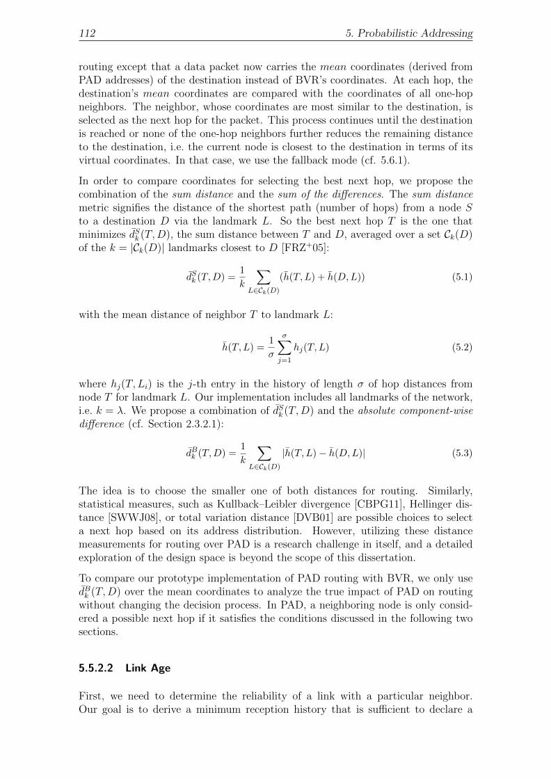
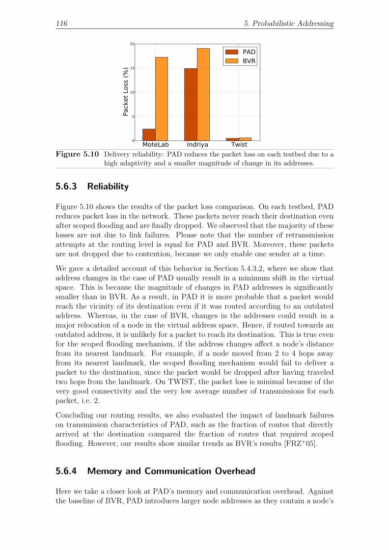
0.35

0.4

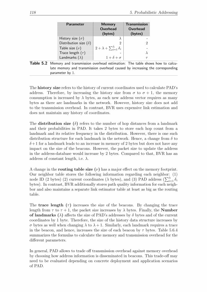
0.45

0 0.1 0.2 0.3 0.4 0.5 0.6 0.7 0.8 0.9 1

Tem

pora

l Sta

ndar

d D

evia

tion

Long-Term Link QualityFigure 2.1 Wireless links exhibit inevitable fluctuations in their quality. The long-

term link quality represent the PRR for entire experimental run. Each datapoint represents the standard deviation in PRR calculated over smaller timeintervals for each directional node-pair. The graph shows data from an IEEE802.15.4 based WSN deployment [ALWB08].

2.1.1.1 Table Management

Besides the accuracy of link quality estimates, an efficient strategy for neighbor tablemanagement is critical in expressing the performance of a link estimator. Tablemanagement typically deals with the following three operations.

Link Insertion: After receiving a packet from a neighboring node, the link estima-tor performs one of the following operations: (1) Update the link quality if the linkalready exists in the table, (2) insert the link in the table if the table is not alreadyfull, (3) ignore the link, or (4) evict a previous entry from the table and insert thisnew link. A link estimator has to carefully choose from these four options ensuringin the meantime that there are enough good links in the table that can be used fordata transmissions.

Link Reinforcement: This operation deals with reinforcing the quality estimateof a link that already exists in the table. The thresholds for link reinforcementprocess, such as how often to perform it, has to be selected carefully to ensurethat the newly calculated link quality does not overshoot or undershoot the desiredaccuracy threshold. Here the main tradeoff is between the agility and stability of thelink quality estimates. Agility means assigning more weight to the recent estimatesfor adapting link quality to the most recent underlying link conditions. However,current link estimators prefer stability over agility by tuning parameters that controlthe history and the weight of the past estimates.

Link Eviction: Finally, a link estimator has to determine when to evict a link fromthe table. Commonly, a time-out or minimum data rate is associated with eachlink to detect node failures and evict corresponding links. Similarly, a minimumquality threshold is typically defined to evict links whose quality declines below thatthreshold. An efficient link eviction policy is important to evict unused links andmake room for new, potentially valuable links in the table.


2.1.1.2 Key Properties

After discussing the basic operational details of link estimators, we now define keyproperties which, in our opinion, are essential for the design of a link estimator.These properties will help us rate the state-of-the-art techniques and shed light ontheir benefits and drawbacks.

• Stability: This property states the stability of the link estimator both interms of link estimates and its ability to support a stable routing topology.

• Adaptability: It determines how quickly the link quality estimates convergeto within the desired accuracy threshold and how well a link estimator adaptsits tables to the underlying link dynamics.

• Current Link State: To see if the link quality reflects the exact link condi-tions at the time of data transmission or if it is only based on past statisticsderived from periodic beacons. This is important because at the time of datatransmission, networking conditions, such as traffic patterns and congestion,can be different.

• Reception Correlation: To determine if packet reception and loss eventsover a link are considered correlated or independent from each other.

• Overhead: The overhead introduced by a link estimator in terms of com-putational complexity, number of transmissions and packet overhearing. Thetransmission overhead includes active link beacons/signalling or additional linkestimation information appended with each data packet. Moreover, packetoverhearing also introduces significant overhead as a node has to receive andprocess packets that are not addressed to it.

2.1.2 Case Studies

We can divide current link estimation mechanisms into two broad categories, long-term and short-term.

In long-term link estimation, link qualities are estimated based on the delivery his-tory of a link. We use the term long-term to emphasize that the focus of suchlink estimators lies on the long-term behavior of a link in the past. In a typicalsetting, each node snoops the channel for ongoing communication in a network,possibly both for periodic beacon packets and data transmissions. The packet lossover a link is inferred by assigning a unique sequence number to packets from eachsource. An ETX value is calculated over a window of size t: If n out of N packetsare received during t then its ETX is N/n. Commonly, an Exponentially WeightedMoving Average (EWMA) is used over the past ETX values with α as a tuning pa-rameter that controls the history of ETX averages. Nodes also exchange their linkestimates with neighbors to aggregate bidirectional link quality. 4BLE [FGJL07],ETX [DCABM05] and BVR’s link estimator [FRZ+05] are among the prominentderivatives of this method.


NetworkNetwork

Pin Compare

Figure 2.2 The 4BLE uses four bits of information: Compare and Pin bit from networklayer, Ack bit from link layer, and white bit from physical layer to enhanceunicast link estimates and table management policy [FGJL07].

On the other hand, short-term link estimation tries to predict the quality of a linkbased on instantaneous conditions. It does not necessarily maintain any recent his-tory of a link but uses current link state (e.g., by sending active probes) to determinelink availability at the time of data transmissions. The supporters of this mechanismargue that the link quality estimates derived from the transmission history of peri-odic beacon packets do not represent the current state of the link. For example, insensornets the network traffic is generated by a rare occurrence of a nondeterminis-tic event. Hence, the channel conditions, such as congestion, experienced by beaconpackets in the past are completely different. SOFA [LKC06], STLE [BLKW08],LOF [ZAS09] and DUTCHY [PH08b] belong to this category of link estimation.

We now present a case study from each of these two categories.

2.1.2.1 Four-Bit Link Estimation

The Four Bit Link Estimator (4BLE) [FGJL07] is a state-of-the-art and classicalexample of a long-term link estimation. It couples link estimation information frombroadcast beacons and unicast data transmission resulting into a hybrid ETX foreach link. Moreover, 4BLE extends traditional ETX based estimation mechanism bycombining information from three different layers – physical, link and network layers– to perform better table management. The key idea behind 4BLE is that each ofthese layers can provide useful information which benefits link estimation process.For example, the network layer can tell which links are most useful for routing andupper layer applications thereby facilitating a link estimator in link insertion andeviction decisions. Similarly, the physical layer can provide channel quality relatedinformation that helps a link estimator in distilling poor links from the estimationprocess. Overall, 4BLE defines four narrow interfaces to retrieve the following fourbits of information – one from physical, one from link, and two from network layers(cf. Figure 2.2):

• Pin: The network layer can pin an entry in the table, preventing the linkestimator from evicting this entry. This bit prevents the link estimator fromevicting a useful entry from the table.


• Compare: It helps resolving inconsistencies between link estimation and rout-ing tables. A link estimator can ask the network layer to compare a newlydiscovered link with an old entry in the table. The network layer responds bysetting the compare bit to suggest that the route provided by the new link isbetter than the link already occupying the table. This bit helps a link estima-tor in identifying progressive link from routing perspective and estimate theirquality instead of wasting critical resources over a useless link.

• Ack: This is the acknowledgement bit set in the transmit buffer if a packettransmission has been acknowledged by the receiver. This bit is used by theestimator to update the corresponding unicast link ETX.

• White: This bit reveals the channel quality per packet. A set white bitindicates high channel quality, which means that each bit in the packet hasa very low decoding error probability. The white and compare bits are usedconjointly to evict entries from the table: If the white bit for a packet receivedover a newly discovered link is set, the link estimator triggers the procedurecorresponding to compare bit in order to decide if this link shall be inserted inthe table by removing a random unpinned entry.

Rating: Figure 2.3 rates the performance of 4BLE against the properties discussedin Section 2.1.1.2. The rating scales from one (low) to five points (high). The positiveor negative meaning of these scales depends upon the property itself. For example,in the case of scalability, a rating of one point means poor scalability, whereas, inthe case of overhead, a rating of 1 point is interpreted as very good, indicating smalloverhead.

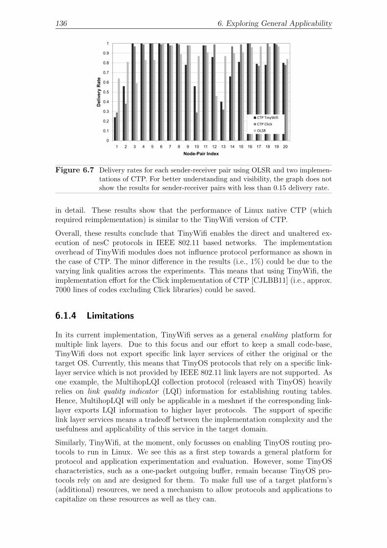
By relying on a long-term delivery history of a link of both broadcast beacons andunicast data transmission and extracting useful information from adjacent layers, the4BLE is by far the most stable current link estimator. CTP [GFJ+09], a widely usedcollection protocol (cf. Section 2.2.2.1), uses 4BLE and outperforms contemporaryapproaches of routing in sensornets by maintaining a stable and a flawless topology.Therefore, it is assigned five points for stability.

4BLE uses an adaptive beaconing mechanism that increases beacon sending rate ifa new node is added to the network or if routing inconsistencies (e.g., loops) aredetected. This mechanism allows 4BLE to quickly converge its link estimates for anewly added link within the error threshold bounds. Similarly, 4BLE reacts quicklyto link failures, i.e., after five failed data transmissions, by disqualifying the linkfor routing purposes. However, the adaptability of the 4BLE is only limited tosuch situations, it fails to quickly recognize the underlying link dynamics to improveperformance [ALL+09, ALW12]: For example, if a previously ignored link becomesreliable and offers a significantly better alternative path than the current links in the

Stability Adaptability Current link state

Stability Adaptability Current link statestate


Reception correlation

Overhead Note

Busty linksy


Overhead Notecorrelation

Short-termestimation


Overhead Note

Long-term estimationestimation

Figure 2.3 The performance rating and the use case for Four Bit Link Estimator.


table, 4BLE is unable to promptly react to such opportunities in the network. Thisis because there are no data transmissions occurring on this link and the adaptivebeaconing slows down exponentially until there are inconsistencies detected in thenetwork. Therefore, it is only assigned two points for adaptivity.

The link estimates in 4BLE are based on past delivery traces and does not regardthe current state of the link. We still assign it one point because it actively monitorsdata path using ack bit and includes this information in calculating link estimates.In general, packet success and loss events over a link are considered independentfrom each other. However, it is assigned 1 point because it disqualifies a link afterjust five failed data transmissions. The overhead of 4BLE is moderate because (1)it only maintains a subset of neighboring nodes in the table for link estimation,and (2) uses active beaconing (link probes) to exchange link estimation informationwith other nodes. However, it does not employ packet overhearing and therefore isassigned 3 points.

2.1.2.2 Solicitation based Forwarding

Long-term link estimation tries to portray what can be expected from a link in thefuture based on how it behaved in the past. However, precisely this approach isits major drawback as well. For example, traffic patterns in sensornets are bursty:The network is in idle state most of the time and only generates large volumes oftraffic when a certain event is detected in the environment. Hence, the link estimatederived from its past transmission statistics, i.e., when the network was in idle state,does not accurately reflect the actual quality of the link at the time of transmission.This is because the traffic patterns and congestion in the network are completelydifferent at the time of traffic burst than when idle. Similarly, the active link probestransmitted when the network is in idle state are illusive and consume needlessenergy.

To address this problem, Lee et. al. present SOFA (SOlicitation based ForwArd-ing) [LKC06] that uses a two way handshake to determine link availability. SOFA isnot just a link estimator but a complete routing infrastructure for low-power wirelessnetworks. However, its major contribution is the link estimation mechanism. Therouting approach of SOFA is based on greedy hop-by-hop forwarding.

SOFA introduces a reactive two-way handshake protocol to determine link availabil-ity at the time of transmission. It does not maintain any other information (e.g.,quality estimates) regarding a link. Each node, when needing to route a packetto sink, broadcasts a request called Solicit-to-Forward (STF). For example, in Fig-ure 2.4, node A sends an STF received by its three neighbors B, C and D. Aneighboring node receiving this message can respond with a reply message calledAccept-to-Forward (ATF). In our example, C is the first node to reply with an ATF.After receiving this reply message, the sender node makes the replying node itsDesignated-Next-Hop (DNH) and starts forwarding its data as shown in the finalstep in Figure 2.4. The DNH is only determined on demand: A timer is associatedwith DNH and once a node is finished sending its packets for the current event andthe timer expires, the node has to redetermine its DNH using the same handshakemechanism. SOFA also employs a passive acknowledgement mechanism: After for-warding a packet, the sender tries to overhear the transmission of its DNH. If it


D D D

A

C

A

C

A

C

A

B

A

B

A

B

STF ATF DNH

Figure 2.4 The two-way handshake in SOFA. Node A sends an STF message. Node Cis the first neighbor to reply with ATF. Node A selects node C as its DNHand forwards data.

overhears the same packet that was recently forwarded, it implicitly assumes thatthe packet has been successfully delivered to the DNH. Otherwise, it retransmitsthe packet until DNH receives it or the maximum number of retransmissions arereached.

An important question is how does a node receiving an STF message determine if itis closer to the sink than the sender node. To this end SOFA assigns height to eachnode so that a receiver node can determine its location with respect to the sendernode. The idea behind assigning heights is remarkably simple once understood.The sink node sends broadcast advertisements which are disseminated in the wholenetwork. The advertisement is initialized with a height of zero (the sink node has zeroheight) and incremented by one at each hop as it propagates through the network.Hence, every node knows its relative distance from the sink node. A sender alwayssends its height in STF and a receiver only replies with ATF message if its heightis less than the sender’s. SOFA also employs height maintenance mechanism ifinconsistencies are observed in the network. For example, if a node’s height becomesa local minimum and no other node is replying with an ATF. This shall never happenin a fully connected network.

In dense networks there may exist a large number of neighbors that can reply withATF. SOFA uses packet overhearing to limit the number of ATF responses. Consideran example with three nodes – A, B and C – each within the communication rangeof the other. Suppose node A wants to send data and thus broadcasts an STF, whichis received by nodes B and C. Lets assume node B replies with an ATF before nodeC does. In this case, node C will snub its ATF because it has already overheard theATF of node B. However, this mechanism only works if the neighboring nodes arewithin the communication range of each other.




Overhead Note

Long-termti tiestimation




Figure 2.5 The performance rating and use case for SOFA.


Rating: Figure 2.5 shows SOFA’s rating. As oppose to 4BLE, SOFA does neitherassigns link estimates nor maintains neighbor tables. Its only contribution towardsstability is the height maintenance mechanism which remedies inconsistent topologydue to high node churn in the network. Therefore, SOFA receives just one pointfor stability. The adaptability of SOFA is similar to 4BLE because it only adaptsits link selection when bad conditions, such as lost transmissions or node failures,occur. However, it does not respond to the opportunities that appear during thecourse of transmission on other, potentially valuable links. For example, in SOFA, ifa neighboring node offers better routing progress than the current DNH, the sendernode will not change its DNH during a transmission burst. Therefore, it gets onlytwo points for adaptability.

SOFA only uses the current link state information and hence it gets maximum pointsfor this property. Similar to 4BLE, packet loss events are in general consideredindependent from each other by SOFA. However, the two-way handshake mechanismextrapolates a notion of packet reception correlation since the last packet delivery(i.e., STF packet) is considered sufficient for the success of succeeding transmissions(two points). Although SOFA does not require link tables for its operation, it hasa very high communication overhead both in terms of the two-way handshake andthe packet overhearing that consumes a significant amount of energy. Especially,the two-way handshake can be detrimental for network performance in challengingnetworking conditions when a node has to repeatedly select its DNH.

2.1.3 Qualitative Comparison with BLE

Both long-term and short-term link estimation mechanisms have their own advan-tages and disadvantages. 4BLE maintains a stable routing topology in the networkat the cost of slow-adaptation to underlying link conditions, i.e., by ignoring progres-sive links that may become reliable during the course of transmission. On the otherhand, SOFA uses the current link state for making its decisions, however, many of itsdesign mechanisms are debatable. For example, in Section 3.4.2, we experimentallydemonstrate that a single successful transmission cannot be considered as sufficientevidence of good link conditions. Moreover, its DNH selection mechanism is veryinefficient: In the case of multiple nodes competing to become DNH, a sender nodeselects a neighboring node as DNH from which it receives the first ATF response.Hence, it ignores the possibility of using other potentially valuable neighbors.

BLE tries to combine the advantages and eliminate the disadvantages of both thesetechniques. We compare BLE with the existing mechanisms by rating it against ourestablished criteria/properties in Figure 2.6. We argue that a stable routing topol-ogy is imperative for establishing reliable and robust routing structures. However,we show that a subtle design of a link estimator that explores transmission oppor-tunities over long range intermediate links does not disrupt the stability of today’s




Overhead Note

Busty linksy




Figure 2.6 The performance rating and the use case for Bursty Link Estimator.


routing protocols. Therefore, BLE does not replace the long-term link estimationbut serves as an additional and modular component that integrates well with existinglong-term link estimation mechanisms. It allows the existing mechanisms to utilizecommunication opportunities that might arise over previously ignored class of linkswithout disrupting the underlying routing topology (Stability = five points). Thedesign and integration of BLE with existing link estimators is discussed in Section3.5.

Similarly, BLE is optimistic in it link selection and allows a routing protocol to adaptto the underlying link conditions both in spreading good news and bad news to theneighboring nodes. The good news represents a situation where a long range inter-mediate link becomes temporarily reliable for transmission. BLE utilizes such oppor-tunities as early as the next three transmissions. Similarly, the bad news representsa situation when an intermediate link again becomes unreliable for transmission.Based on empirical observations from multiple testbeds, BLE avoids overshootingan unreliable link by reverting back to a high quality link even if a single transmis-sion fails over an intermediate link (Adaptability = four points, Current Link State= five points). BLE thresholds for qualifying or disqualifying a link are discussed inSection 3.4.2.

The key idea behind the development of BLE is to break the assumption of inde-pendent packet reception events over a link. It measures the quality of a link interms of its burstiness that shows the correlation of packet reception events over alink (Reception Correlation= four points). This information is essential in deter-mining if a link is useful for packet forwarding or not. To make this concept clearlet us consider two links, one which rarely transmits a packet successfully and theother which alternates between reliable and unreliable transmission periods, i.e., itis bursty. Approaches such as SOFA cannot differentiate between these two linksbecause they do not employ any mechanism to determine if the previous successfultransmission occurred by chance or if this link is bursty. Similarly, it is unlikely that4BLE will utilize this link because of its poor ETX estimate in the long-term. BLE’slink estimation metrics are discussed in Section 3.4.

BLE is based on passive overhearing of packets and does not require active linkprobes. However, it is an extension rather than a replacement of existing long-termlink estimation mechanism. Therefore, in addition to the underlying link estimator,such as 4BLE, it incurs additional overhead of packet overhearing and link estimatecalculation (Overhead = four points). Section 3.5.3 gives details regarding BLE’soverhead.

2.2 Routing

A link estimator is only concerned with a node’s one hop neighborhood. Routingprotocols establish multihop structures using link estimation information at eachhop. In this section, we discuss some of the prominent routing approaches in sen-sornets. We also define key properties of a routing protocol and compare differentapproaches with our proposed extensions.

2.2. Routing 19

0 10 20 30 40 50 60 700

0.1

0.2

0.3

0.4

0.5

0.6

0.7

0.8

0.9

1

Feet

ReceptionSuccessRate

EffectiveRegion

TransitionalRegion

Clear Region

.Figure 2.7 Reception rates vs. distance between nodes in a line topology: In the ef-

fective region all links exhibit good to perfect quality. The quality fallssmoothly as the distance between nodes grow (transitional region) and even-tually degrading to very poor link quality (clear region) [WTC03]

2.2.1 Introduction

Unlike wired networks, shortest path routing based on hop-distance metric is notfeasible in wireless networks because a wireless link between two nodes reveals moredynamics than simply being considered available or not. For example, a link withPRR = 40% may deliver enough routing updates to be considered for data pack-ets, thereby resulting in a significant number of retransmissions to deliver a packet.Figure 2.7 clarifies this observation further by showing the relationship between linkreception quality and the distance between communicating nodes. Links from tran-sitional and clear regions can dominate route selection because they offer betterrouting progress. However, using these links without assessing their reception qual-ity leads to unstable routing topology, frequent retransmissions, and poor routingthroughput.

In order to deal with these problems, contemporary routing protocols typically em-ploy ETX [DCABM05] as a routing metric to establish high throughput paths be-tween distant nodes. Path establishment in multihop wireless networks is usuallybased on distance vector routing approach: The participating nodes are not aware ofthe complete network topology. They only know the next hop that leads towards aparticular destination and the routing cost along the path offered by that hop. Linkstate routing mechanisms have also been optimized for multihop wireless settings(e.g., OLSR [CJ03]), however, they are typically not preferred in large scale set-tings for two reasons, (1) limited scalability, and (2) inherent limitations of wirelessdevices (especially in sensornets) in terms of computations, storage and energy.

Routing approaches in wireless networks can be categorized in two broad categories,address free and address based. In address free routing, a node is typically assigneda unique identifier. It is mostly suited in situations where point to point commu-nication is not relevant such as in data collection and dissemination in sensornets.Data flows in address free routing can be many-to-one or one-to-many. On the otherhand, address based routing is needed for point-to-point communication scenarios


RR’s communication range

1 1.5

3

R

1 1.5A’s communication range

BA

C

3A

C

1.2

1.5

B

D D

Step 1 Step 2Step 1 Step 2

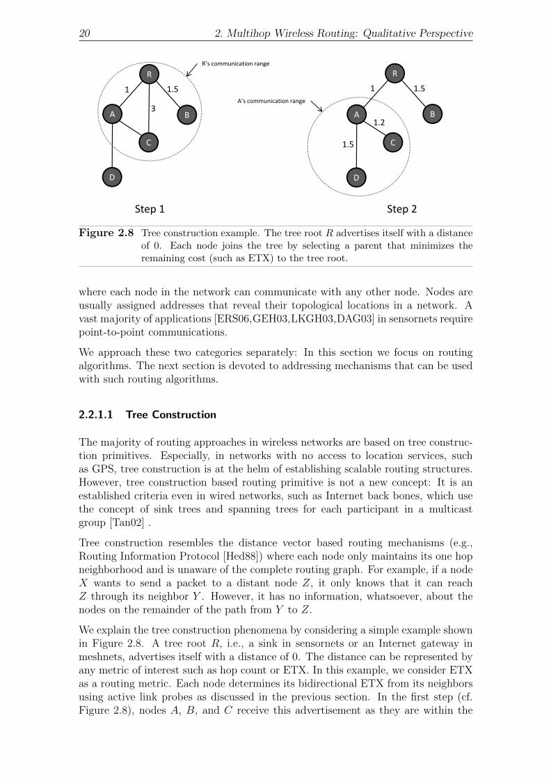
Figure 2.8 Tree construction example. The tree root R advertises itself with a distanceof 0. Each node joins the tree by selecting a parent that minimizes theremaining cost (such as ETX) to the tree root.

where each node in the network can communicate with any other node. Nodes areusually assigned addresses that reveal their topological locations in a network. Avast majority of applications [ERS06,GEH03,LKGH03,DAG03] in sensornets requirepoint-to-point communications.

We approach these two categories separately: In this section we focus on routingalgorithms. The next section is devoted to addressing mechanisms that can be usedwith such routing algorithms.

2.2.1.1 Tree Construction

The majority of routing approaches in wireless networks are based on tree construc-tion primitives. Especially, in networks with no access to location services, suchas GPS, tree construction is at the helm of establishing scalable routing structures.However, tree construction based routing primitive is not a new concept: It is anestablished criteria even in wired networks, such as Internet back bones, which usethe concept of sink trees and spanning trees for each participant in a multicastgroup [Tan02] .

Tree construction resembles the distance vector based routing mechanisms (e.g.,Routing Information Protocol [Hed88]) where each node only maintains its one hopneighborhood and is unaware of the complete routing graph. For example, if a nodeX wants to send a packet to a distant node Z, it only knows that it can reachZ through its neighbor Y . However, it has no information, whatsoever, about thenodes on the remainder of the path from Y to Z.

We explain the tree construction phenomena by considering a simple example shownin Figure 2.8. A tree root R, i.e., a sink in sensornets or an Internet gateway inmeshnets, advertises itself with a distance of 0. The distance can be represented byany metric of interest such as hop count or ETX. In this example, we consider ETXas a routing metric. Each node determines its bidirectional ETX from its neighborsusing active link probes as discussed in the previous section. In the first step (cf.Figure 2.8), nodes A, B, and C receive this advertisement as they are within the

2.2. Routing 21

radio range of root R. As this direct link is the only choice currently available toreach R, in the next step, nodes A, B and C make R as their parent and replicatethis advertisement, however, by respectively changing ETX values to 1, 1.5, and 3.In the second step, node D receives advertisements from both A and C and computesits path ETX as follows:

my ETX to neighbor <X> + ETX from <X> to R. (2.1)

Suppose both links−−→DA and

−−→DC are of the same quality, D selects A as its immediate

parent as the path over this node is clearly optimal. However, in this step C alsoreceives the advertisement of A and realizes that using a single hop to reach R ismore costly in terms of ETX than using A as a relay node. Therefore, it selects nodeA as its new parent and uses the new ETX value for subsequent advertisements. Thisprocess continues with the hope that ETX of a link will not change dramatically anda stable tree will be established with all nodes in the network joining the tree byselecting their parents. Tree construction suffers from typical distance-vector routingpathologies such as count to infinity, loops, and stranded nodes [Tan02]. Routingprotocols employ mechanisms to recover from such pathologies. For example, loopsare detected if a packet exceeds the maximum allowed number of hops specified inthe time-to-live field.


Now we define key properties to establish a base for a fair qualitative comparison ofrouting case studies with our proposed routing extensions. Most of these propertiesare similar to link estimation properties discussed in the previous section, however,their definitions are extended at the network level instead of just a node’s one hopneighborhood.

• Stability: Similar to link estimation, stability points to the steadiness of arouting topology and how gracefully a routing protocol recovers from node andlink failures in the network.

• Adaptability: It determines how well a routing protocol adapts to the un-derlying link conditions, i.e., by responding to link estimator’s suggestions, toenhance performance parameters such as throughput and number of transmis-sions.

• Scalability: It shows the maximum stretch of the routing topology in terms ofhow many nodes can be supported in the network without any communicationbreakdown. This is one of the most important properties for routing protocolsin sensornets because the envisioned scale of deployment surpasses thousandsof cooperating networked objects (motes).

• Reliability: The delivery rate of a routing protocol. It is one of the mostimportant measure of routing performance in multihop wireless networks.

• Overhead: Routing overhead is measured in terms of transmission, i.e., thefrequency and size of routing update messages, and storage, i.e., the memoryrequired for maintaining routing structures such as routing tables.


2.2.2 Case Studies

From service point of view, we can divide routing protocols in wireless networksin two broad categories: proactive and reactive. As the name suggests, proactiverouting protocols actively establish routing topology once a network is in place anda protocol is activated irrespective of if the applications really want to send data.Hence, such protocols maintain a connected network at any time. CTP [GFJ+09],MintRoute [HSNW10], OLSR [CJ03] are among the examples of proactive routingprotocols.

On the other hand, reactive routing protocols are demand based and only establisha route when two nodes intend to communicate with each other. Once the com-munication is over, the routes are typically disabled after a certain period of time.These protocols are specifically useful in challenging networking conditions and mo-bility scenarios when maintaining an active routing topology is costly. DSR [JM96],AODV [PBRD03] and DYMO [BY09] are well known examples of reactive routingapproaches.

We will now discuss three case studies: (1) CTP, state-of-the-art proactive routingin sensornets, (2) Opportunistic routing [BM05a, BM05b], a novel approach of ex-ploiting link diversity in meshnets, and (3) AODV, a widely used reactive routingapproach used both in sensornets and MANETs. Although this dissertation doesnot directly connect with reactive routing approaches, we present a case study herefor completeness.

2.2.2.1 Collection Tree Protocol

CTP [GFJ+09] is one particular instance of collection tree protocol described in [RGJ+06].It is state-of-the-art and one of the most widely used collection protocols shippedwith TinyOS [LMG+04,LG09], an OS platform for sensornets implemented in nesClanguage [GLvB+03a,GLvB+03b]. It uses 4BLE as its link estimator.

The basic operational principle of CTP is the same as distance vector based treeconstruction discussed earlier. However, it uses some novel mechanisms to addresstwo common problems of distance vector based approaches; (i) loops, and (ii) slowresponse to topological changes [Tan02]. The former is clear, however, the laterrequires some explanation. In distance vector routing, any news (e.g., node additionor breakdown), spreads across a network very slowly, one hop per update interval. Soa node cannot be fully incorporated or removed from routing decisions until the newshas spread across the whole network. Decreasing the update interval is a straightforward solution to spread the news quickly, however, it generates unnecessary trafficwhich is prohibitive in energy constrained sensornets. In order to address theseproblems, CTP introduces the following two mechanisms.

Datapath Validation: Typically, routing protocols use update messages to detectloops. However, CTP actively monitors data packets to solve any discrepanciesalong the data path. Each packet carries the transmitter’s local ETX estimate to thedestination, calculated using the mechanism discussed in Section 2.2.1.1. Logically,the ETX of the recipient node shall always be less than the ETX value in the receivedpacket. This is because the transmitter will only send a packet to its parent that is

2.2. Routing 23

closer to the destination than itself. A packet is considered to be in loop if it violatesthis rule, i.e., its ETX is less than or equal to the receiver’s ETX. Consequently, thereceiver node initiates data path validation instead of simply dropping the packet.The data path validation deals with updating the ETX estimates of an out-of-datenode using adaptive beaconing.

Adaptive Beaconing: As already mentioned, the sending frequency of routing up-dates (beacons) is a tradeoff between resource consumption and the recentness ofthe topology. CTP introduces an adaptive beaconing mechanism to strike an effi-cient tradeoff between the two. Using this mechanism, in emergency situations –such as addition/deletion of a node or loop detection – the network can respondwithin milliseconds by aggressive beaconing, while slowing it down significantly innormal conditions to save energy and bandwidth. The adaptive beaconing is a mod-ification of Trickle [LPCS04] algorithm used for disseminating code updates in thenetwork. In Trickle, a node suppresses its update and doubles the update-intervalif it overhears a similar update, or decreases the update-interval to the minimumwhen it receives a new code update. Similarly, adaptive beaconing mechanism ex-pands or shrinks a node’s beaconing interval based on stable or unstable topologicalconditions in a network, respectively.

Rating: Figure 2.9 qualitatively evaluates CTP on functionality accounts. It isa very stable collection protocol based on long-term link estimation and efficientlyrepairs discrepancies in its routing topology. Therefore, we assign it four points forstability. The adaptivity of CTP stems from 4BLE: It changes a degrading link afterjust five failed transmissions. However, it is unable to use valuable opportunities onlinks that are black-listed by the link estimator due to their dynamic and burstynature. Nonetheless, quick recovery of the topology using adaptive beaconing earnsit two points.

CTP only maintains a constant number of neighbors, all one hop neighbors atmaximum, in the routing table irrespective of the network size and node density.Therefore, it achieves high scalability (four points) as demonstrated by empiricalevaluations in [GFJ+09]. The reliability of CTP is well proven as it has been thor-oughly tested on twelve testbeds using six different link layer protocols [GFJ+09].It delivered more than 90% of the packets on all testbeds with different physicaltopologies and varying link conditions, and hence, we assign it 4 points for its relia-bility. Finally, the overhead of CTP accounts for (1) the routing beacons exchangedamong the neighboring nodes using the adaptive beaconing mechanism discussedearlier, and (2) the routing table, which maintains the state of a subset of one hopneighbors of a node.

Stability Adaptability Scalability Reliability Overhead Note

Proactive collection

Figure 2.9 The performance rating and use case for CTP.


2.2.2.2 Opportunistic Routing

Opportunistic routing (or ExOR) [BM05a, BM05b] comes closest to BRE both interms of how it operates, and its ambition of exploiting long range intermediatelinks in meshnets. Similar to BRE, ExOR does not operate as a stand alone routingprotocol. It tries hard to forward packets over intermediate links that offer betterrouting progress and are closer to the destination. However, after delivering 90%of the packets in a batch, it uses the reliable delivery mechanism of an underly-ing routing protocol, such as OLSR, for delivering the remaining packets over thetraditional path. In a similar fashion, BRE extends the ability of the underlyingrouting protocol to exploit intermediate links. There are two key differences be-tween opportunistic routing and BRE: (1) The former uses broadcast primitive andthe next forwarder (i.e., next hop) of the packet is determined among the receiversof a packet using an agreement protocol. The later uses unicast transmissions im-plying that the next forwarder of the packet is predetermined. (2) BRE aggressivelyreverts to traditional routing to avoid overshooting an unreliable intermediate link.However, ExOR operates on a batch of packets and tries very hard to deliver 90%of the packets before returning to traditional routing.

ExOR is based on the idea of cooperative diversity [vdM77] that uses broadcasttransmissions to forward information through multiple relays. The destination canthen use the best received signal or even combine information, i.e., to reconstruct thesignal, received via multiple relays. ExOR utilizes two unique opportunities of linkdiversity in multihop wireless networks. First, using broadcast packet transmissions,it utilizes intermediate nodes along the traditional routing path to forward packets ifthe transmission falls short of the intended recipient. This way, the progress alreadymade by a packet is utilized since an intermediate node, instead of the sender, for-wards the packet further. Second, the packet may travel farther (e.g., 2 hop distance)than the intended recipient. ExOR makes use of this luck by providing mechanismsto allow farthermost recipient of the packet to become the next forwarder instead ofthe intended recipient.

Figure 2.10 explains the basic idea behind ExOR: Lets assume node A wants tosend a packet to node D. In traditional routing, it forwards the packet to node C,the next hop in the routing table for node D. Suppose node C fails to receive thistransmission but node B does. ExOR utilizes this opportunity by allowing node Bto deliver this packet either directly to node D or via its next hop. Similarly, in thesecond case, the transmission from node A might occasionally be received by nodeD directly. ExOR also allows the routing protocols to take advantage of this goodfortune.

In the following, we discuss the three main operational ingredients of the oppor-tunistic routing protocol.

Determining the forwarder set: ExOR determines a prioritized subset of nodes thatshall be responsible for receiving and forwarding the packet. To compute the for-warder set, ExOR requires knowledge about the loss rate of each link in the network.In the first step, a sender node calculates the shortest path to the destination. Thefirst node in this path gets the higher priority to forward packets. The same pro-cedure is repeated to complete the forwarder set by deleting the previously selectedcandidates from calculations and assigning lesser priority to the node that is selected

2.2. Routing 25

A B C D

Good Intermediate Bad

Figure 2.10 A simple example explaining the cooperative diversity utilized in oppor-tunistic routing. Packets from node A to node C might occasionally bereceived by destination D directly or by node B. ExOR exploits suchopportunities by avoiding retransmissions from node A.

in the later step. This forwarder set is then cached until the next link-state update.Each packet contains its forwarder list in the header.

Agreement protocol: The nodes in the forwarder set then use an agreement protocolto forward the packet. ExOR operates on batches of packets to minimize the over-head of the agreement protocol. The main purpose of the agreement protocol is toschedule the time when a node should transmit its fragment of the batch. Higherpriority nodes, as indicated by the forwarder set, are allowed to transmit first. Anode maintains a forwarder timer that is scheduled far ahead to allow higher prior-ity nodes to transmit first. This timer is readjusted when the node overhears othernode’s transmission. Each node also maintains a batch map that determines, foreach packet, the highest priority node known to have received that packet. Theagreement protocol heavily relies on packet overhearing to update batch maps.

Reliable delivery : ExOR does not offer reliable delivery. Therefore, it uses the tra-ditional routing as a backup mechanism, which employs hop-by-hop acknowledge-ments, for delivering the lost packets requested by the destination.

Rating: ExOR uses ETX based routing topology maintained by an underlyingrouting protocol. Therefore, we assign it 4 points for stability (as we did in thecase of ETX based CTP’s topology). Rating ExOR’s adaptability is not straightforward: Although its performance is heavily dependent upon the underlying linkcondition, it does not pay any specific attention to varying link conditions at therouting layer. Nonetheless, it employs a highly efficient algorithm for packet forward-ing that prioritizes the next hop selection; with the node closest to the destinationalways being assigned the highest priority. In short, ExOR’s algorithm ensures thatevery progress made by a packet during a single transmission is utilized withouttaking link dynamics directly into consideration (Adaptability = 3 points).

ExOR doest not scale well because it needs link-state information of the wholenetwork. Therefore, we assign it only 1 point for its limited scalability. ExOR itself


Cooperative diversity

Figure 2.11 The performance rating and use case for ExOR.


S D S D

Route request propagation Route reply propagationFigure 2.12 Route request and reply propagation through the network in AODV.

does not guarantee reliable delivery. However, the use of traditional routing as abackup ensures that it is at least as reliable as the traditional routing itself. Hence,it is assigned 4 points for reliability. The biggest limitation of ExOR is the overheadassociated with its agreement protocol that includes (1) forwarder lists and batchmaps appended with each transmitted packet, (2) packet overhearing to updatenode state, and (3) the computation complexity of the protocol itself. Therefore,weassigned 5 points for its high overhead.

2.2.2.3 AODV

In Section 2.2.2.1, we discussed CTP that has been specifically designed to meetthe stringent resource constraints of sensornets. Similarly, in the previous section,we discussed ExOR that exploits wireless link diversity. However, ExOR is quiteexpensive both in terms of computational and transmission overhead and hence itis not suitable for resource constrained sensornets. AODV, on the other hand, is amore general reactive routing approach: It was originally designed for MANETs andlater adapted to sensornets. Reactive routing approaches are useful in challengingnetwork conditions where maintaining a consistent routing topology is expensive. Forexample, in a network with mobile nodes (e.g., MANETs) or limited connectivitybetween nodes due to harsh environmental conditions (e.g., sensornets). As thisdissertation does not target reactive routing approaches, therefore, we will be verybrief in our description of AODV. There are three steps in AODV’s reactive routingapproach, (1) route request (2) route reply, and (3) route maintenance.

Route Request: In AODV, each node maintains a small table containing information,such as a set of neighbors to forward packet to, for a particular destination. Linkswith neighbors are generally considered available or unavailable. Hence, it does notperform any active link estimation.

The route discovery in AODV proceeds as follows: When a source S wants to senda packet to destination D, it looks up its table to see if there is a neighbor entry fornode D. Route discovery is only initiated if it does not find an entry in the tablefor node D. The same procedure is repeated at every intermediate node. When anentry for node D is not found, node S broadcasts a ROUTE REQUEST packetrelayed by all its neighbors until it reaches the destination or an intermediate nodethat already has an entry for node D in its table. Figure 2.12 explains this processby showing the paths taken by the ROUTE REQUEST packet to reach node D.

2.2. Routing 27

Route Reply: When a route aware intermediate node or destination D receives therequest it replies with a ROUTE REPLY packet. However, this ROUTE REPLYpacket is now unicasted along the same path over which it was received – the smallestpath is chosen if multiple requests are received – in the opposite direction (cf. Figure2.12). As this packet traverses through the network, each intermediate node recordsan entry for node D for to establish a distance vector. Once this packet is receivedby the source of ROUTE REQUEST packet, it initiates its data communicationwith node D.

Route Maintenance: Node mobility can cause sudden changes in the network topol-ogy. Therefore, a node has to keep track of which routes in the table are valid fromtime to time. In this regard, a node regularly exchange HELLO messages, to which,each of its neighbor is suppose to respond. If a response message is not received, allthe associate entries for the non responsive neighbors are deleted from the table.

Rating: AODV is a customized routing protocol only feasible in specific scenarios,i.e., networks with high node mobility. It does not match the stability of proactiverouting approaches as routes are established based on simple route request andreply primitives. There is no link estimation performed and hence low quality linkscan dominate AODV’s route selection without any particular consideration given totheir feasibility for data transmission. Hence, it only receives 1 point for its stability.AODV treats links as available or unavailable, giving no consideration, whatsoever,to the underlying changes in link quality. It is assigned 1 point for its adaptabilitybecause of its route request and reply mechanism that allows for path reconstruction.

Longer tables with multiple forwarding candidates for each destination and an ex-pensive route discovery mechanism strongly limit the scalability (1 point) of AODV.A number of studies [GSAP06, YIM+08, Kle08, DA10, CAAKA10] have been per-formed to implement and evaluate AODV in different classes of wireless networksunder varying networking conditions. The reported reliability results of AODV dif-fer significantly (e.g., from < 50% [Kle08] to > 90% [PRD99]) due to difference inevaluation environments. Similarly, the lack of link estimation makes it more sus-ceptible to long range links of bad quality. The inclusion of such links results infrequent route discovery across the network due to frequent transmission failures onunreliable paths. Therefore, we assign it only 2 points for reliability.

Finally, it has a very high overhead (5 points) both in terms of memory footprint andbandwidth consumption due to frequent exchange of HELLO messages and routerequests. However, it is clear that AODV targets specific ad hoc communicationscenarios with high node mobility.


Reactive On-demand

Figure 2.13 The performance rating and use case for AODV.


2.2.3 Qualitative Comparison with BRE

Today’s routing protocols in wireless networks use similar techniques as in wirednetworks [PB94, CJ03, BM05b, DPZ04]. They construct tree like topology and re-strict communications to a very limited set of paths, typically a single path be-tween two communicating nodes. These paths are constructed based on high qual-ity links identified by a link estimator. Hence, today’s routing approaches are pes-simistic and conservative in their link selection and only achieve suboptimal routingprogress [BM05b, RSBA07a]. This results in heavy utilization of a selected set oflinks and paths even though there is a multitude of other potentially useful pathsavailable in the network.

BRE extends existing proactive routing approaches by providing relevant supportto utilize link diversity inherent in wireless networks. It provides relevant supportat the routing level to include intermediate links, i.e., recommended by BLE, in therouting process. In doing so, BRE allows traffic to be distributed among differentlinks, relieving heavily congested paths and nodes. Similar to ExOR, BRE is oppor-tunistic in its link selection and always prefer long range links before falling back totraditional routing algorithm. Hence, it would not be unrealistic to state that BREis a simpler yet efficient variant of ExOR.

Figure 2.14 shows BRE’s relative rating when compared to the existing routingapproaches. BRE presents an adaptive routing strategy that allows a node to switchamong different parents based on link estimation information while maintaining oneprimary parent as a backup. These changes in parents, however, are strictly localand do not impact the overall routing topology in the network. Therefore, it achievesthe same stability as traditional proactive routing approaches (Stability = 4 points).Sudden changes in parent allows a node to adapt its next hop selection to veryrecent network conditions and exploit interesting opportunities over intermediatelinks. Nonetheless, BRE only promises optimal link selection within a node’s onehop vicinity but does not promise optimal path in the network (Adaptability = 4points). We discuss BRE’s parent selection and adaptability in Sections 4.4.1 and4.4.3, respectively.

BRE does not alter the stability of proactive routing approaches because it neithermaintains any additional routing table nor exchanges further routing updates (Scal-ability = 4 points). Moreover, the design of BRE is highly modular and is not tiedto any specific routing protocol. It integrates well with different routing approachesand link estimators. The scalable design of BRE is discussed in Section 4.4.

Similarly to ExOR, BRE maintains the packet delivery reliability of traditional rout-ing approaches (Reliability = 4 points). In Section 4.5.3.2, we show that it evenimproves the packet delivery ratio of traditional routing in challenging network con-ditions by selecting best links based on instantaneous channel conditions. Finally,


Long-range forwarding

Figure 2.14 The performance rating and use case for Bursty Routing Extensions.

2.3. Addressing 29

the only additional overhead introduced by BRE is its lightweight algorithm (Over-head = 4 points). We discuss BRE’s overhead in Section 4.5.6.

2.3 Addressing

Point-to-point communications in multihop wireless networks require an address-ing scheme to locate nodes in the network. Many addressing schemes have beenproposed both for sensornets and meshnets such as geographical [IN99, BMSU99,KK00, KWZZ03], hierarchical [Tsu88a, Tsu88b, EFK07] and virtual coordinate ad-dressing [CA06, FRZ+05, MOWW04, JS03, RRP+03]. However, our main focus liesin self-configurable and decentralized addressing schemes which are equally relevantin multiple classes of wireless networks. Therefore, in this section, we concentrateon addressing schemes that derive virtual node locations based on the underlyingconnectivity in a network.

2.3.1 Introduction

There are two main ingredients of point-to-point communication in multihop wirelessnetworks, addressing and routing. Addressing deals with assigning locations to nodesin the network topology. A far located sender node uses this address for routingpurposes. Routing on the other hand deals with actual decision making at eachnode to select the best next hop for the packet to reach its destination. In general,routing is performed greedily to allow for a scalable communication infrastructurethat only requires a node to know its one hop neighborhood.

2.3.1.1 Challenges

Assigning locations to nodes in a multihop wireless network is a complicated task.As opposed to wired networks, there is no permanent network infrastructure thatcan be manually configured beforehand. Many factors contribute to rapidly changingtopologies in a network such as node breakdown due to battery depletion in sensor-nets and a large number of participants moving, leaving, or joining the network inMANETs.

Traditional addressing schemes, such as IP, greatly suffer if applied to multihop wire-less networks. For example, IP based hierarchical addressing is not feasible becauseit requires a very careful manual configuration of the entire network assuming astatic topology. Unlike wired network, an IP address of a node in a wireless networkis merely used to identify a node in the network for Internet communications but itdoes not reveal the routable location of the node. Another solution is geographicaladdressing that also requires either manual configuration or GPS support. However,in wireless networks, the connectivity graph is dynamic and strongly depends on thephysical environment. Therefore, a geographical path leading towards a node mightnot be the optimal path based on the connectivity graph. Similarly, geographicrouting suffers heavily from holes (or dead ends [YLRT09,LLM06]) in the network.


In recent years, virtual coordinates based addressing schemes have received much at-traction in the research community for two main reasons: First, they are completelydecentralized and self configuring. It means that nodes determine their addressesthemselves after joining the network without any central coordination or manual con-figuration. Second, these schemes are based or the underlying connectivity graph,and hence, a node’s address guides the packets to follow the best path leading to-wards the node. These benefits of virtual coordinate-based addressing mechanismsmake them suitable for both sensornets and meshnets. Before presenting a few casestudies on virtual coordinate-based addressing schemes, we identify the key proper-ties of an addressing scheme in a wireless network.


Following are the key properties of an addressing scheme that we use to comparestate-of-the-art case studies with our proposed approach PAD.

• Address Stability: This property states the number of times a node changesits address. Address changes may occur due to (1) variations in the underlyinglink conditions, or (2) frequent node failures. It is an important propertybecause a node’s location is typically stored in a distributed global databasein the network and every change in the address requires an update in thatdatabase. Hence, address update is an expensive operation.

• Address Monotony: Once an address change occurs, this property deter-mines the magnitude of difference (e.g., in hop counts) between a node’sprevious and new location. A smaller change in address (i.e., high addressmonotony) could result in higher routing success even if the packets are routedtowards the destination using its outdated addresses. This is because the pack-ets may still reach the vicinity of the destination whose new location is veryclose to the old one.

• Resilience: It shows how well an addressing scheme recovers from frequentnode additions and departures from the network. In such dynamic scenarios,a resilient addressing scheme would require far less address updates in thenetwork than a non-resilient one.

• Scalability: This is similar to routing scalability in the previous section. Itshows the ability of the addressing scheme to enlarge itself to accommodatethe growing number of nodes in the network.

• Overhead: It is measured in terms of storage requirements and control pack-ets, such as beacons or address updates in the global database, exchanged tomaintain stable addressing in the network.

2.3.2 Case Studies

In this section, we present two well known case studies of point-to-point routing,namely BVR [FRZ+05] and S4 [MWQ+10]. BVR is one instance of virtual coordi-nates based addressing specifically implemented for sensornets. S4 is a cluster basedextension of BVR that achieves significantly smaller routing stretch than BVR.

2.3. Addressing 31

421X(2,4,4) (4,4,3) (4,4,1)

3(3,5,4)(0,4,5)

5 6 7 8 Z(2,2,3) (3,3,2)(1,3,4)(2,4,5) (4,5,0)

Y 9 1211(3,1,4) (4,2,3) (4,3,2) (5,4,1)

10(4,0,5)

Figure 2.15 Virtual coordinates based addressing in BVR. Each node determines thehop distances from landmarks in the network. A vector of these hop dis-tances, i.e., virtual coordinates, is used as a node’s routable address.

2.3.2.1 Beacon Vector Routing (BVR)

BVR is also based on tree construction primitive. However, it needs multiple treeseach rooted at landmark. A landmark is a designated node in the network usedas a reference point by all other nodes. Every node in the network identifies itsposition in each landmark tree. The location of a node is defined in terms of a vectorof hop distance from each landmark, commonly referred to as virtual coordinates .Routing is performed greedily over the virtual coordinates. There are two operationalingredients of BVR, virtual coordinate based addressing and routing.

Virtual Coordinates: Figure 2.15 shows an example of BVR’s virtual coordinatebased address establishment in a network with three tree roots (landmarks). Land-marks advertise themselves by repeatedly sending beacons. Based on these beacons,each node S (recursively) determines the number of hops h(S, Li) to each land-mark Li. The result can be viewed as a set of routing trees with the landmarksas their roots and with, for example, the hop count as a routing metric. A nodeS’s coordinates ~c(S) in the virtual coordinate system are the λ-dimensional vector< h(S, L1), . . . , h(S, Lλ) > with λ as the total number of landmarks. In our examplein Figure 2.15, node 7 has a three-dimensional address vector < 2, 2, 3 > where eachvector component represents the node’s hop distance to the landmarks X, Y , andZ, respectively.

Routing: Routing is performed greedily over these addresses. The idea is to let anode S choose a next hop T that minimizes the remaining distance d(T,D) to thedestination D (e.g., select a neighbor as a next hop whose coordinates are most sim-ilar to those of the destination node). BVR uses absolute component-wise differenceas a routing metric:

d(T,D) =λ∑i=1

|Ti −Di| (2.2)

However, real-world deployments are confronted with lossy links that may falselyinfluence the hop distance from landmarks. It means that traversing one hop canrequire more than one transmission. Therefore, the “best” next hop is the one thatresults in the least number of transmissions necessary to reach the destination. BVRemploys a link estimator to identify neighbors with stable links that minimizes ETX


for a successful delivery. Thus, only a selected subset of neighbors – offering anETX below a certain threshold – are used in calculating the hop distance from thelandmarks. Nonetheless, a node’s address vector still represents the hop distanceover the path with minimum ETX.

Rating: Figure 2.16 rates the performance of BVR. The address stability of BVRstrongly depends upon the underlying network conditions. Tree construction offersa simple and attractive addressing solution, however, it is increasingly difficult tomaintain stable trees in challenging network conditions. Changes in a particularnode’s coordinates propagate throughout the network and trigger further changesdown the tree. For example, if a node close to a landmark changes its coordinatecomponent for that landmark, all the descendant nodes will have to change theircoordinates as well. Therefore, we only assign two points to BVR with regard toaddress stability.

The magnitude of change in node’s coordinates (address monotony) is calculatedby summing the absolute component-wise difference of each coordinate component.The idea is to see if changes in a node’s coordinates are sudden or gradual. AsBVR’s tree construction process is based on long term link estimation, it stronglylimits the number of options for reaching landmarks and this usually results in ahigher magnitude of change in addresses. For example, a node may change its hopdistance from two to four (magnitude of change = two points) for a certain landmarkbecause this is the best option available among the set of limited neighbors with highquality links. Hence, BVR is only assigned 2 points for its address monotony.

BVR is not particularly resilient to address changes because it is unable to locallyrecover from node additions or failures [FRZ+05]. Thus, node dynamics lead tosignificant changes in the topology throughout the addressing tree (resilience = onepoint). The scalability of BVR is comparable to any other tree construction basedrouting approach, such as CTP. However, the state maintained per node is notconstant and depends upon the number of landmarks in a network (scalability =three points). Besides state maintenance at each node, BVR relies on expensivepacket overhearing based link estimator that appends link estimation informationwith each outgoing packet (Overhead = four points).

2.3.2.2 Small State and Small Routing (S4)

S4 is a cluster based extension of BVR that significantly reduces routing stretch.S4 argues that the attempts to maintain small state per node to achieve higherscalability can result in undesirable routing performance in terms of routing stretch– the ratio of the hop count of selected path to that of the optimal path [MWQ+10].It minimizes both the state and routing stretch by combining the distance-vectorbased global network state and scoped distance-vector based local cluster state. S4

Stability Monotony Resilience Scalability Overhead Note

Virtual coordinates

Figure 2.16 The performance rating and use case for Beacon Vector Routing.

2.3. Addressing 33

DF

L EC

D

L

Nodes with E in their cluster

B

AA

Figure 2.17 S4’s routing scenarios. (1) A → C: B intercepts packets from A to deliverthem directly to C instead of traversing through landmark L. (2) A →E: No shortcut is found and the packet is delivered via landmark (e.g.,BVR’s case). (3) D → C or F → E: Shortest path routing is used as thedestinations are within the local cluster of sender nodes [MWQ+10].

achieves an average routing stretch of 1 and is the state-of-the-art point-to-pointrouting protocol in sensornets.

Algorithm: Apart from maintaining global virtual coordinates in the network, as inBVR, each node in S4 maintains a routing table for all the nodes in its local cluster.A node S’s local cluster Ck(S) contains all the nodes whose distance to D are withink times their distances to their closest landmarks. The idea behind maintaininga local cluster is that a node S can intercept packets addressed to node D anddeliver them directly (cf. Figure 2.17). This significantly reduces the routing stretchbecause the packet does not have to reach the closest landmark of the destination,and then from there to the destination itself.

One of the key advantages of S4 is its small addresses. As opposed to BVR, therouting approach of S4 does not require the whole coordinate vector to be included asdestination’s address in the packet header. For packet forwarding, a node’s addressis nothing but the ID of its closest beacon. If a node wants to send a packet toanother node within its cluster, it directly forwards the packet to the destinationover the shortest path. However, if a sender node from another cluster sends a packettowards the destination’s closest landmark, the packet is either intercepted by anintermediate node with destination in its cluster or it finally reaches the landmarkand then delivered to the destination. Figure 2.17 depicts multiple routing situationsand shows how S4 reacts in each of these situations.

Optimizations: Maintaining two level topological structure requires robust mecha-nism both for maintaining both inter-cluster and intra-cluster topology. S4 intro-duces relevant mechanisms to ensure a stable topology at both levels. For inter-cluster routing each node is supposed to know its (shortest-path) distance to all thelandmarks in the network. Therefore, a reliable delivery of beacon packets (adver-tisements) initiated by landmarks is necessary to maintain a stable topology. Thisis because sudden packet losses can sometimes result in miscalculation of the dis-tance while other times may require substantial changes in the topology, thereby


degrading the performance of S4. To address these challenges, S4 requires everynode S in the network to rebroadcast beacons until n neighbors have received it orthe maximum retransmission count tmax has reached. The choice of tmax and n is atradeoff between the overhead and reliability.

Similarly, for intra-cluster routing, a node S has to retransmit a packet until anacknowledgment is received or the maximum retransmission count has been reached.In the later case, S initiates a local failure recovery request. After receiving thisrequest, S’s neighbors try to recover the packet locally. The idea is to select a nodethat is closest to the destination as the next hop for S. To avoid an explosion oflocal failure responses, in case a large number of S’s neighbors maintain a distancevector for the destination in their tables, a prioritized response mechanism based ontheir distance vector is used. This way, each neighbor knows how long it has to waitbefore sending a failure recovery response.

Rating: The main difference between BVR and S4 is that the latter achieves smallerrouting and transmission stretch. However, with regard to the properties definedfor our qualitative comparison, S4 gathers a similar rating as BVR for scalability,monotony and resilience, as shown in Figure 2.18. Although S4 needs to maintain aglobal and local state per node, it can be as scalable as BVR by carefully selectingthe state bounds. Similarly, address monotony remains the same because globalvirtual coordinates of S4 are based on BVR’s distance vector approach. Recoveringfrom node failures is at least as troublesome as in BVR. S4 achieves slightly higherstability than BVR because of its beacon rebroadcasting mechanism. Finally, theoverhead of S4 is similar to BVR [MWQ+10].

2.3.3 Qualitative Comparison with PAD

Virtual coordinates, such as in BVR, offer an attractive addressing mechanism formultihop wireless networks whose deployments are often unplanned and lack anypermanent network infrastructure. However, their direct adoption of tree construc-tion primitive is not as efficient as in address-free collection protocols (cf. Section2.2.2.1). This is because in virtual coordinate addressing both addressing and rout-ing are strongly coupled with each other: A change in a node’s immediate parentdoes not only impact the routing path towards a tree root but also the routable lo-cation of that node and all its descendants. Hence, link quality changes along a treebranch (path) force virtual coordinate based addressing mechanisms to recomputeaddresses of all the nodes connected to the tree via that branch. This limitationstrongly impedes the routing performance despite high overhead for regular addressupdates in challenging network conditions.

In PAD, a node’s virtual coordinates are expressed in the form of probability dis-tributions. We introduce a degree of fuzziness in a node’s address that acclimatizes


Routing stretch

Figure 2.18 The performance rating and use case for S4 protocol.

2.3. Addressing 35

short-term changes in the underlying link conditions. For example, if a node knowsthat it can reach a landmark in the network over multiple paths, it will not deriveits coordinate component for that landmark by selecting the best path in terms ofthe offered quality and the number of hops. Rather, it will represent its coordinatecomponent in the form of a probability function that expresses a subset of pathstowards landmarks and the relative frequencies at which these paths are available.Hence, PAD doest not maintain any explicit trees in the network and automaticallysupports the inclusion of intermediate links into the routing process by embeddinginformation regarding multiple paths leading towards a node in its address distribu-tion. Thereby, a node’s topological location is no longer dependent on a particularpath but on a subset of such paths. As a result, link quality changes along a singlepath does not necessarily change the location of the nodes along that path sincethese nodes are reachable over multiple paths.

Figure 2.19 provides a comparative rating for PAD. One of the key advantages ofPAD is its stability (4 points). Because it assigns fuzzy address to nodes instead ofsharp coordinates, PAD concedes a degree of error in its addresses. Later in Section5.4.3.1 we show that PAD achieves an order of magnitude higher address stabilitythan BVR and S4. Section 5.4.2.2 discusses error tolerance in this fuzzy addressingscheme.

PAD achieves a very high address monotony (4 points) because it is neither de-pendent on stringent tree like topology nor on expensive link estimation. Hence,unlike BVR, which depends upon robust parent selection predominantly influencedby routing cost metric and link estimation, PAD lessens the need for this stringentparent-child relationship in a network. A node in PAD does not have a static posi-tion but a region where it can reside just like an electron resides in its region aroundthe nucleus of an atom. As long as a node is within its assigned region, it canbe reached without needing to change its coordinates. The same reasons apply foraddress resilience: Since a node is no longer dependent on a single parent, a sud-den departure of a node does not necessarily impact the location of its descendant.However, in BVR, the importance of a node grows with regard to address resiliencedepending upon (1) how close it is to a landmark, and (2) how many descendantsit holds in the tree. For example, the departure of a node closer to a landmarkcan break the whole routing tree associated with that landmark and inflict addresschanges throughout the network. We shed light on PAD’s address establishment,resilience and monotony in Sections 5.3.2, 5.4.3 and 5.4.3.2, respectively.

Despite its long addresses, PAD achieves similar scalability as BVR and S4. First,because it only maintains a subset of routes leading towards landmark in its addressdistribution regardless of the node density (cf. Section 5.3.2). Second, because itoffers a number of design choices with regard to address establishment, aggregationand dissemination in the network. For example, one such scalable design choice


Fuzzy coordinates

Figure 2.19 The performance rating and use case for PAD.


LinkEstimation Stability Adaptability

4BLE

SOFA

BLE

Routing Stability Adaptabilityg y p y

CTP

E ORExOR

AODV

BRE

Addressing Stability Monotony

BVR

S4S4

PAD

Current link state

Reception correlation Overhead

Scalability Reliability Overheady y

Resilience Scalability Overhead

Figure 2.20 Summary of the performance rating assigned to case studies in the area oflink estimation, routing, and addressing.

would be to aggregate PAD addresses in the form of mean or weighted average anduse them for routing purposes. Section 5.5 discusses these concepts of aggregatingPAD addresses.

The main overhead of PAD is its long addresses. However, when compared with BVRand S4, PAD neither employs packet overhearing nor link estimation for establishingaddresses in the network. Therefore, we assign it a similar rating (Overhead = 4points). The overhead of PAD is discussed in Section 5.6.4.

2.4 Summary

In this chapter, we discussed link estimation, routing, and addressing concepts inmultihop wireless networks. We also presented state-of-the-art case studies from eachof these three areas and conceptually compared them with the protocol extensionsproposed in this dissertation. Figure 2.20 summarizes our comparison. We canclearly see that BLE, BRE, and PAD enhance different performance characteristicsof existing approaches.

Long term link estimation is the preferred mechanism employed by today’s linkestimators. Its primary goal is to establish a stable routing topology. However, inachieving this goal, it mainly disregards packet reception correlation and the currentstate of a link at the time of packet transmission. 4BLE adds a degree of adaptiveness

2.4. Summary 37

to this estimation technique by demoting a link immediately after five consecutivepacket failures. This helps in improving routing reliability but contributes littletowards our goal of utilizing long range intermediate links in the network. Contrarily,short term link estimation primarily focuses on the current link state but achieveslimited stability – a primary routing design requirement. BLE tries to combine theadvantages of both these approaches. It does not underestimate the need of stablerouting topology, while at the same, provides relevant mechanisms to estimate longrange intermediate links and utilize them for packet forwarding.

Routing protocols typically utilize high quality links for packet forwarding. The ideais to convert the network graph into a simplistic tree like structure and only use thelinks that form the branches of that tree. In doing so, they limit packet forwardingto a very limited set of links. ExOR provides an elegant solution to efficientlyutilize link diversity and the broadcast nature of wireless medium. However, itscomputational requirements and reliance on link-state information for each directedlink in the network limits its usage to resource rich platforms such as in meshnets.BRE provides an alternative and light-weight solution to exploit link diversity. Ithas a transparent design that can integrate well with existing routing approachesand does not introduce any changes in the protocol building blocks such as packetheaders.

Virtual coordinate based point-to-point routing approaches are also unable to ex-ploit link diversity to ensure long term stable addressing in the network. Despitea tremendous emphasis on address stability, these approaches suffer from frequentaddress updates in dynamic network conditions. In this regard, PAD provides a so-phisticated solution to address both these problems. A PAD address is composed ofmultiple paths leading towards a node and also exposes the quality of these paths inthe form of a probability distribution. Moreover, it assign fuzzy locations to nodesto account for sudden changes in link conditions and thus maintain stable address-ing across the network even under challenging network conditions. In the followingchapters we discuss the design and evaluation of BLE, BRE and PAD in detail.


3Estimating Link Burstiness

After introducing the problem space and establishing a formal discussion backgroundin the previous chapters, we now turn our focus towards the actual contributions ofthis dissertation. We begin with our first contribution, i.e., link estimation, whichforms the basis for including intermediate links into the routing process.

In the previous chapter, we learned that the prevalent approach in proactive routingalgorithms is to employ a link estimator that identifies high quality links for packettransmissions. The use of intermediate links is thus disregarded (except if thereare no high quality links in a network), although these links provide considerableadditional resources for routing. This is because sudden changes in their transmissionsuccess rate make it difficult to accurately estimate the quality of such links andpredict the fate of future transmissions [MRBT08]. Another reason for the exclusionof intermediate links from the routing process is their poor ETX estimates calculatedover a longer period of time. We argue that ETX is not an optimal metric toexpress the nature of such links at short time scales. In particular, bursty links posea major challenge to existing link estimation mechanisms [AWK+11b]. Estimatinglink burstiness and the length of successful transmission bursts is pivotal in assessingthe utility of these links from a routing perspective. Therefore, we need a specializedlink estimator to estimate intermediate links.

Based on significant empirical evidence of over 100,000 transmissions over each linkin widely used IEEE 802.15.4 and IEEE 802.11 testbeds, we propose two metrics,EFT and MAC3, for runtime estimation of bursty wireless links. We introduce anew link estimator (BLE) that, based on these two metrics, accurately estimatesbursty links in a network rendering them available for packet transmissions. BLE isoptimistic in its link selection and prefers long-range intermediate links over short-range stable links.

The rest of this chapter is structured as follows. Firstly, we motivate the problemspace and discuss related work in Sections 3.1 and 3.2, respectively. We then analyzeand define the exact scope of our work in Section 3.3. From this, we derive the designof our metrics and show their viability in Section 3.4. Finally, Section 3.5 presents

40 3. Estimating Link Burstiness

the design and evaluation of our link estimator before we summarize the discussionin Section 3.6.

3.1 Motivation

The availability and reliability of wireless links exhibit dynamic behavior at shortand long time scales [LCL07,KCPnC09]. Therefore, choosing the best link, in termsof routing progress and the need for transmission resources, requires an accurateand timely estimation of the available links. Current link estimators, using metricslike PRR and ETX, only capture link dynamics at long time scales for the sake of astable routing topology. These metrics estimate the quality of a link over extendedperiods of time – in the order of minutes – and thus achieve poor estimates forrapidly changing bursty links. As a result, such links are typically excluded from therouting process. However, recent protocol studies [ALL+09,BM05a,WTC03,PH08a]demonstrate that these links are long range and achieve significantly higher routingprogress than stable links. Using these links therefore covers otherwise multipletransmissions and thus saves the energy and resource consumption coupled withthese transmissions. Furthermore, previous studies [Zan97, SDTL06a] have shownthat typical traffic patterns in the Internet as well as in multihop wireless networksare bursty. Hence, an optimal online link estimation at the time of a burst benefitsspontaneous transmissions as well as the overall network performance.

Link burstiness is a well established fact: It has been thoroughly analyzed [ABB+04],accurately modeled [KCPnC09], and experimentally measured [SKAL08]. In burstylinks, shifts between phases of reliable and poor packet delivery occur at short timescales, but future packet delivery is correlated to the recent success rate. Despiteestablishing a very strong knowledge base regarding the causes of link burstinessover the past few years, we still lack metrics that define the quality and usability ofbursty links. Similarly, we need a link estimator that can assess link usability online(i.e., at runtime) to enable the inclusion of these links in the routing process.

3.1.1 Link Categorization

Until now we have been using indeterminate terms, such as good or bad links, to referto the different types of links based on their transmission quality. Before digginginto the details of our link metrics, we believe that it is essential to formally definethese terms for the sake of better understanding of the concepts presented in thisdissertation. All the link categories defined in Table 3.1.1 are not new. Similar termshave been used in the literature previously [SKAL08,Sri10].

The three categories that we specifically define for this dissertation are bursty, inde-pendent and unused links. To the best of our knowledge, the only formal definitionof link burstiness is provided by Srinivasan et. al. [SKAL08]. Our definition of linkburstiness slightly differs: We want to estimate link burstiness at runtime, whilethey try to measure link burstiness offline for understanding link behavior to finetuning protocol parameters. Hence, our definition of a bursty link is biased towards(1) the utility of a link for packet transmission, and (2) a metric that can be calcu-lated at protocol runtime. Therefore, we define a link as bursty if one can predict

3.1. Motivation 41

Category DefinitionGood PRR > 90%Intermediate 10% < PRR < 90%Bad PRR < 10%Bursty CPDF(3) > 75%Independent CPDF(3) < 75%Unused Any of the above links not

used for routing purposes

Table 3.1 Link categorization: A link estimator tries to identify good links in a network.Bursty links show correlated packet delivery and one can predict the fate of futuretransmission with high probability. An unused link is not employed by routingprotocols for reasons like bad link quality estimate or absence of a link from therouting table due to strong table-size restrictions.

the fate of future transmission over that link with high probability (using a verylimited delivery history of that link). We use Conditional Packet Delivery Functions(CPDF (n)) [LCL07] to predict the success probability of the next transmission. Wedefer a more detailed discussion on CPDF (n) and the thresholds chosen in Table3.1.1 for defining bursty links to Section 3.4.2. Any non-bursty intermediate link isindependent.

The unused category refers to all the links in the network that, for some reason,are not used by the routing protocol for packet forwarding. The reason could be asmaller table size, the inefficiency of a link estimator or the routing protocol, or theresulting poor estimates of that link.

3.1.2 Requirements

The requirements and challenges of estimating intermediate links are substantiallydifferent from conventional link estimation discussed in Section 2.1. For example,long-term packet reception rates – otherwise the key link quality metric – of inter-mediate links do not suffice as a metric. Rather, we are interested in the followingthree pieces of information:

• Whether or not packet delivery on an intermediate link is correlated to itsrecent delivery history, i.e., if the link is bursty or independent? It is importantbecause any transmission attempt over an independent link could be comparedto mere gambling with an unknown chance of success.

• How long a bursty link remains reliable for transmission, i.e., what is the lengthof successful transmission bursts? It is important because a bursty link thatonly momentarily becomes reliable for transmission triggers frequent switchingamong links, degrading the overall routing performance.

• When a bursty link has a reliable or unreliable transmission period? We needto pinpoint exactly when a reliable/unreliable transmission sequence occursover bursty links to ensure their effective utilization.

None of these three pieces of information, which we consider keys to profitably usingintermediate links for routing, are provided by existing link estimators.


3.1.3 Major Contributions

The definition of appropriate metrics for estimating intermediate links and the designof a link estimator based on these metrics are the main contributions of this chapterand our major departure from the existing work. The contributions are summarizedas follows:

• We introduce MAC3 as a metric to estimate the burstiness of links based onrecent delivery traces. MAC3 extends the established CPDF [LCL07] by cal-culating a moving average over the results of CPDF (Moving Average CPDF ).

• We define EFT as a metric to estimate the duration for which a bursty linkremains reliable for transmission. We also show that EFT is strongly correlatedto MAC3.

• Based on these two metrics, we introduce BLE, derive requisite parameters forits usage, and evaluate its efficacy in estimating intermediate links. Our resultsindicate that BLE identifies bursty links in the network with high accuracy,hence paving the way for including such links in the routing infrastructure.

3.2 Related Work

Capturing link dynamics at different time scales and characterizing link burstinesshave been the focus of many recent studies. We can divide prominent related effortsinto three main categories.

3.2.1 Measuring Link Burstiness

In their seminal study on quantifying the extent and characteristics of bursty links,Srinivasan et. al. [SKAL08] define a factor β that measures the burstiness of awireless link. β is calculated by using CPDF (n) [LCL07,SKAL08] that determinesthe success probability of the next transmission after n consecutive successes orfailures. Hence, β is used to differentiate between bursty links with long bursts ofsuccesses or failures and links with statistically independent packet losses – withperfectly bursty and completely independent links marking the opposite ends of thespectrum.

Although β is a very useful metric to measure link burstiness, it is primarily usedto characterize link burstiness based on existing traces rather than online assess-ment. It is statistically very complex to compute and requires a long delivery his-tory (e.g., 10,000 packets) to accurately measure link burstiness. Our evaluation inSection 3.4.3 also reveals that calculating β over short history sizes, a fundamentalrequirement for online assessment, results in fluctuating and error-prone results.

3.2. Related Work 43

3.2.2 Short Term Link Estimation (STLE)

In our preliminary work on wireless link dynamics [BLKW08, ALWB08, Bec07], weintroduced the packet snooping based concept of STLE to analyze the impact of therecent transmission success and failure rate on the future quality of a link at fine-grained time scales. However, although STLE is concerned with link estimation,we argue that the proposed mechanism only provides link discovery: STLE onlytells whether or not a link becomes temporarily available but does not provide anestimation for how long this will be the case [Gra10]. Furthermore, no differenceis made between recurring bursty links and accidental successful deliveries. Thesecharacteristics cause STLE to repeatedly select a link even if packet transmissionsover that link frequently failed in the previous attempts. This further impedes itsusability in real-world networks.

Approaches such as Solicitation-based forwarding (SOFA [LKC06]) remove the needfor long-term link estimation and test link availability by sending a short hand-shakepacket as a probe before sending any data packets. However, our evaluation in Sec-tion 3.4.2 shows that a successful hand-shake should not be taken as a success guar-antee for subsequent data transmissions and indicates a need for more sophisticatedmodels.

3.2.3 Long Term Link Estimation (LTLE)

This is the traditional link estimation mechanism employed by the majority of cur-rent multihop wireless routing protocols [GFJ+09, FRZ+05]. It is based on win-dow mean exponential weighted moving averages (WMEWMA) of link PRRs orETX [DCABM05]. Although this metric is highly accurate and has a small settlingtime for good and bad links, i.e., with PRRs close to 0% and 100%, it does not per-form well for links of intermediate quality [WTC03] – also indicated by our resultsin Section 3.5.1. Hence, such link estimation mechanism cannot be used for esti-mating intermediate links at short time scales. However, these links often offer thehighest routing progress [CWK+05b] suggesting the need for more precise estimationmethods.

The assumption underlying the majority of existing link estimation concepts isthat packet loss events over a link are independent from each other (i.e., they fol-low a Bernoulli distribution). This assumption has been challenged before in re-search [CWPE05, SDTL06b]. The analysis of our data in Section 3.4 supports thehypothesis that the assumption of independent packet losses is not appropriate atthe fine-grained time-scales dealt with in this dissertation.

Table 3.2 highlights the main operational differences between existing link estima-tion mechanisms and our proposed solution. We use 4BLE [FGJL07] and SOFA asreference implementations for our comparison.

3.2.4 Estimating Multiple Link Properties

Both STLE and LTLE mechanisms estimate the quality of a link based on a singlelink property, such as PRR, ETX or RSSI. The argument used to develop link


Property 4BLE SOFA BLEPassive overhearing × X XTable management X × XLink history X × XHandshaking × X ×Estimation metric X × XUnicast estimates X × X

Table 3.2 Operational differences between link estimators. Handshaking refers to link levelconnection establishment before data transfer. Unicast estimates specify the abil-ity of a link estimator to monitor data traffic for link estimation purposes.

estimators based on multiple link properties [SKB10,REWT11,KS06] is that a singleproperty is not sufficient to approximate the presumed future behavior of a link.

F-LQE [SKB10] combines four link properties, namely packet delivery, link asymme-try, stability and channel quality into a single hybrid estimate calculated using fuzzylogic [NW05,Har00]. A fuzzy subset [Tan96] of good links is defined using these fourproperties. The F-LQE link quality indicates the membership of a particular linkwith this fuzzy subset. Although the authors demonstrate the superiority of F-LQEover existing LTLE mechanisms, it does not meet our design goals of estimatingintermediate links. This is because it complements the existing LTLE mechanismsby combining four properties of links that do not reveal the key characteristics ofintermediate links such as link burstiness.

Renner et. al. [REWT11] argue against the use of a single-value metric for expressingthe quality of a wireless link. This is because a single-value metric only presents asnap-shot of a particular link property at any particular instance of time. It is unableto express the variation trend both in long- and short-term behavior of the link inthe past. They propose a Holistic Packet Statistics (HoPS) concept, which providesdetailed information about static and dynamic behavior of a link using four distinctlink quality values namely short-term estimation, long-term estimation, absolutedeviation and trend. HoPS achieves higher fidelity than existing link estimationtechniques and can improve decision making at higher layer protocols such as routingand topology management. However, the short-term link estimates in HoPS arebased on PRR and thus they do not provide the required information that we believeis mandatory for exploiting intermediate links.

3.3 Problem Analysis

To provide a clear motivation for our work as well as a separation from the previouslymentioned related work, we now define our problem space and the requirements for asolution. First, we motivate the need for employing a new link estimator in networkswhere LTLE mechanisms are prevalent. Second, we explain the basic concept ofour approach by considering a simple example. Based on this, we highlight the keyrequirements of a link estimator for incorporating bursty links in the routing process.

3.3. Problem Analysis 45

1

Good links (quality > 90)

0.6

0.8

DF

Good links (quality 90)

Intermediate links

0.4

CD (10 < quality > 90)

Bad links (quality < 10)

0

0.2

0 10 20 30 40 50 60 70 80 90 100

(q y )

PRR (%)Figure 3.1 The cumulative distribution of different types of links in a wireless network.

A considerable amount of links show intermediate to bad quality. The graphshows data from an indoor grid-like deployment of 36 TelosB motes (cf.Section 3.4.1).

3.3.1 The Need to Utilize Bursty Links

With regard to the characterization of links in [SKAL08], LTLE mechanisms typi-cally utilize only good to perfect links with a PRR ≥ 90%. However, most links inwireless networks exhibit worse PRRs and are thus excluded from routing decisions(cf. Figure 3.1). Although this approach results in a stable and a clear-cut routingtopology, it results in heavy utilization of the selected links that typically offer alittle routing progress on each hop. In LTLE, a trade-off is thus made between thehigh cumulative resource consumption of series of short range links and the ease ofutilizing only a fraction of the existing links. In contrast to this, bursty long-rangelinks offer high routing progress with only one transmission but need to be includedin the routing process. For example, Figure 3.2 compares the probabilities of findingan intermediate link or a good link when the distance between sender and receivernodes increases. It clearly shows that the probability of finding an intermediatelink is higher in particular at longer distances. However, the utility of these linksdepends upon an accurate online estimation, which is not possible using today’s linkestimators.

In multihop wireless networks networks, such as sensornets and meshnets, the net-working hardware is the most dominant consumer of energy. The amount of en-ergy consumed by the networking hardware is directly proportional to the num-ber of transmissions required by a packet to reach its destination. By utilizingbursty links with significantly better routing progress (i.e., less number of hops tra-versed) [BM05a, ALL+09], the number of transmissions and thus, the amount ofenergy consumed can be reduced.


0.8

0.9

1Good Link

Intermediate Link

0.5

0.6

0.7

babi

lity

0 1

0.2

0.3

0.4

Pro

b

0

0.1

0 2 4 6 8 10 12 14 16 18 20

Distance (m)Figure 3.2 Distance vs. probability of finding a particular link category. The proba-

bility of finding an intermediate link is higher when the distance betweennodes increases (cf. Section 3.4.1 for data set).

3.3.2 Basic Concept

We construct a simple example to understand the requirements of estimating inter-mediate links. Consider a linear topology of nodes A , B, C, and D as depicted inFigure 3.3. Node A can reach node D via multiple paths such as A→ B → C → D,A → C → D and A → D. Using ETX as link metric, indicated by labeled-edgesin Figure 3.3, a traditional link estimation and routing approach will always useA → B → C → D as the only path between nodes A and D. This approach ispessimistic in its link selection because it does not consider the opportunities thatmay appear during the course of consecutive transmissions on other links, such asA → C or even A → D, by persisting with stable links. Hence, this approach iswilling to concede performance penalties to avoid sudden changes in link estimatesand routing paths.

An optimistic approach, on the other hand, will speculate the fate of transmissionson long-range intermediate links (e.g., A → C and A → D). This is because if thetransmission over such a link is successful, it can potentially reduce the total numberof transmissions required by packets from node A to node D. One such optimisticyet expensive approach is ExOR (cf. Section 2.2.2.2), which lets a broadcast packetto be received by a subset of nodes. These nodes then decide on a candidate thatforwards the received packet. For example, if both nodes B and C receive thetransmission from node A, node C shall forward the packet because it is closerto node D. However, creating such an understanding among node subsets requiresmaintaining link-state information at each node in the network. Hence, this approachis both expensive and less scalable.

3.3. Problem Analysis 47

2.5 2.7

A B C D1 1.1 1.2

3.8

Figure 3.3 Explaining the concept of utilizing intermediate links with a simple example.The labels show the corresponding ETX of the edge.

Another approach is to first seek for an intermediate link, and if the transmissionover this link fails, deliver the packet over the traditional path. This dissertationargues in the favor of this approach for two reasons:

• It is simple and based on unicast communication.

• It is distance vector based and therefore, unlike ExOR, does not require eachnode to maintain the link-state of the whole network.

However, exploiting an intermediate link for transmission without assessing linkconditions at the time of transmission confronts one of the following two cases.

• If the intermediate link is independent then the fate of future transmissions overthis link cannot be predicted. Hence, any speculative transmission attemptover this link will reciprocate to its overall ETX measured by a traditional linkestimator.In other words, a 40% link is expected to deliver only 40% of thepackets successfully. Hence, using such a link for packet transmission is notdesired.

• if the packet loss events over an intermediate link are correlated, i.e., the linkis bursty, then the fate of a future transmission depends upon the time whenthe transmission attempt is made. As a matter of luck, a 40% link may deliverup to 80% of the packets without any retransmissions, if these attempts aremade during the reliable delivery period of that link. In the contrary case, a40% link may deliver less than 10% of the packets.

This dissertation tries to substantiate this luck by enabling the nodes to attempta transmission over an intermediate link only if it is bursty and precisely at thetime when it is showing good transmission characteristics. Hence, in the case ofFigure 3.3, if node A possesses this knowledge, it can utilize links A→ C and A→D. Estimating link burstiness during runtime and discovering reliable transmissionperiods over an intermediate link is our main goal in this chapter.

3.3.3 Design Goals

The design of a link estimator that reliably reflects the state of a given link has tofulfill multiple requirements.


Characteristic Mirage ComSysMotes Micaz TelosBRadio chip CC2420 CC2420Environment Indoor IndoorArea 160’ x 40’ 45’ x 45’Tx. power 0 dbm -25 dbmInter packet interval 10 ms 6 msBurst length 100000 3000Channel 26, 11 26

Table 3.3 Transmission characteristics for Mirage and ComSys datasets.

• Appropriate metrics need to be derived as key building blocks of the estimator.Such metrics must timely estimate the current link quality based on a veryshort transmission history, in order to adapt to the rapidly changing reliabletransmission periods of bursty links. Additionally, the predicted link qualitymust accurately and reliably reflect the actual link quality, i.e., the estimationerror needs to be small and stable.

• Building upon such metrics, a link estimator must efficiently utilize the giveninformation to select beneficial links for routing. This requires appropriateneighbor table management policies that select those links for routing – amongall the available links – which allow for the best routing progress.

• The link estimator mechanisms should be lightweight and resource sensitive interms of computation, storage, and communication. For example, frequentlybroadcasting beacons to estimate a link on a short-term basis is prohibitivebecause it consumes significant amount of energy and bandwidth, the two mostcritical resources in sensornets.

3.4 Deriving Metrics for Bursty Links

Based on the properties specified in the previous section, this section defines andevaluates two metrics, MAC3 and EFT, that (1) identify bursty links in a networkand (2) estimate the length of successful transmission bursts. These metrics sub-sequently lay the foundation for BLE. In the following, we first provide detailedinformation on the particular data set used in the remainder of this study.

3.4.1 Data Set and Experimental Model

The design of our link quality metrics as well as the resulting BLE are based onwidely used empirical data rather than a theoretical model. We strongly believethat empirical observations from multiple real world scenarios are important bothfor developing metrics and evaluating the efficacy of the concepts presented in thisdissertation. Although attempts have been made previously, it is difficult to capturetransmission fluctuations and the dynamics revealed by intermediate links only usinga theoretical model [SKAL08,LCL07,KCPnC09].

3.4. Deriving Metrics for Bursty Links 49

The evaluation results presented in this chapter are based on two different datasets.First, the SING mesh data-set [Dat09] compiled at Stanford University and usedin many recent state-of-the-art studies [SKAL08, SJC+10, Sri10] on wireless linkdynamics. It is a comprehensive data set collected from multiple IEEE 802.11and IEEE 802.15.4 testbeds1 including both packet and byte level radios such asTexas Instrument’s CC2420 [Ins07] and CC1000 [Chi02]. Second, the ComSysdata set from Becher et. al. [BLKW08], collected from an indoor deployment of36 TelosB [PSC05] motes. Unless otherwise noted, our evaluation shows resultsfrom Mirage testbed [CBA+05] – a 100 node MicaZ [SA08] testbed at Intel ResearchBerkeley. Specifically, the data comprises traces of transmissions on IEEE 802.15.4channel 26 at a transmission power level of 0 dBm. Out of all available links, weonly include intermediate links in our analysis and comparison. This is becausegood links would measure highly in our metrics and would thus improve our results.However, these links are not the focus of our work.

Table 3.4 lists the important characteristics of our data set. The burst length indi-cates the number of packets broadcast by one node before passing on this duty tothe next sender in the network.

3.4.2 Predicting Transmission Success from a Short History

Before introducing our metrics MAC3 and EFT we motivate our goals and approachwith a case study. We address the question, whether a short history of successfultransmissions is sufficient to predict with a high probability that the next transmis-sion on this link will be successful, too. Our goal is to find a minimum thresholdthat is sufficient to predict the fate of future transmissions.

Figure 3.4(a) depicts the conditional probability of a successful packet transmissionbased on the average long-term link quality (i.e., PRR) and a short-term history of alink. It shows that for a link with a long term quality greater than 60%, even a singleor two successful transmissions over that link raise the success probability of the nexttransmission to 90%. Similarly, it shows that for any link, regardless of its long termlink quality, the probability of a future successful transmission is greater than 90%if the last three packets over that link were sent successfully. Figure 3.4(b) depictsthe probability of a successful packet transmission based on the average long-termlink quality and a short-term history of consecutively failed packet transmissions.It indicates that after one or two consecutive losses any link should be temporarilyconsidered unreliable.

Overall, these results indicate that a short-term history of three packets over a linkis sufficient to determine with a high probability whether the next transmission willbe successful or not. Hence, from this case study, we derive a history of 3 packets asa suitable threshold for discovering reliable periods of transmission over bursty links.A smaller threshold value, such as 1 or 2 packets, is risky as it does not guaranteea successful delivery over an intermediate link. Similarly, using a larger thresholdvalue, such as > 3 packets, does not significantly increase the success probability offuture transmissions while impeding the prediction process.

1MoteLab [WASW05], Mirage [CBA+05], and SWAN [Sta] testbeds. Please visit http://sing.stanford.edu/srikank/datasets.html and the websites of each testbed for further information,e.g., topology, connectivity etc.

http://sing.stanford.edu/srikank/datasets.html

http://sing.stanford.edu/srikank/datasets.html


00.10.20.30.40.50.60.70.80.91

0.80.7

0 1 2/ 3 2 3/ 4 4/ 5 3 5/ 6 4 5 6

Success History (n)0

0.20.4

0.60.8

1

Long-Term Link Quality

0

0.2

0.4

0.6

0.8

1

CPDF(n)

(a) Influence of the recent transmission success rate on the success probabilityof the next transmission.

00.10.20.30.40.50.60.70.80.91

01

2/ 32

3/ 43

4/ 54

5/ 65

6

Failure History (n)

0

0.2

0.4

0.6

0.8

1

Long-Term Link Quality

0

0.2

0.4

0.6

0.8

1

CPDF(n)

(b) Influence of the recent transmission failure rate on the success probabilityof the next transmission.

Figure 3.4 Measuring the impact of recent transmission success or failure over a link onthe next transmission over that link. A label of k/n stands for k successesduring the last n transmissions, and n is a shorthand for n/n. CPDF(n)is the probability that the next transmission is successful. Long term linkquality reflects the PRR, calculated over the whole link trace.


(a) h = 3

(b) h = 4

Figure 3.5 Conditional packet reception probability of two distinct history sizes, (a)h = 3 and (b) h = 4. The probability is shown for all possible combinationsof packet loss and reception events (first row) for a particular history size.Symbols 0 and 1 represent packet loss or reception event (first column), re-spectively. The radius of the circle scales with the probability of a particularevent [Bec07].

Figure 3.5 precisely illustrates the packet loss and success probability of the nexttransmission for all possible combinations of packet loss and success events usingtwo distinct history sizes (i.e., h = 3 and h = 4). We can clearly see that h = 3suffices for predicting the success probability of next transmission.

In the following, we introduce two metrics MAC3 and EFT that determine thesuccess probability of future transmissions on a per link granularity, hence allowingus to reflect spatial properties of link dynamics.

3.4.3 Online Estimation of Link Burstiness

Estimating the burstiness of a link is mandatory to determine whether or not anintermediate link is beneficial to the overall routing performance. The key challengeis to clearly distinguish intermediate links with correlated packet losses from thosewith independent losses. However, unlike offline measurement mechanisms like β,we are not interested in how close a link is to an ideal bursty link with one longburst of either successes or failures. Our goal to predict link burstiness at runtimestrongly influences the definition of burstiness and the timescale of our prediction.In this context, we define a link to be bursty as long as we can recurrently predict thefate of only the next transmission over a link with high probability. This is why weintroduce a new metric that monitors a link for a limited transmission history andexpresses if the occurrence of a successful transmission burst over a particular linkis a mere coincidence or if it is a reoccurring trend. This information is importantto determine if a link is beneficial for routing purposes.


ϒ = 1 ϒ = 0

A: 1 1 1 1 1 1 1 1 1 1 0 0 0 0 0 1 1 1 1 0B: 1 1 0 1 1 1 1 0 0 0 1 0 1 1 1 0 1 1 1 0

Variables Link A Link B

ρ 10 4

ϒ = 1 8 1

ϒ = 0 2 3

CPDF(3) 8/10 = 0.80 1/4 = 0.25

Figure 3.6 Calculating CPDF(3) for two contrasting links. Link A has a higherCPDF(3) and is more suitable for routing.

3.4.3.1 MAC3

Our online metric Moving Average CPDF (MAC3) is based on CPDF (n) whichcalculates the probability of one successful transmission following n previously suc-cessful transmissions. Based on the results in the initial case study in Section 3.4.2,we compute CPDF (3) over the recent history h of length m of a link:

CPDF (3) =

∑mi=1 γi|ρ|

(3.1)

ρ defines the total occurrences of three consecutive successful transmissions in thehistory. For example, in a transmission history 111001, there is only a single validoccurrence of three consecutive successful transmissions. γ is a boolean functiondefined as follows:

γi =

{1 if hi = 1 ∧ hi+1 = 1 ∧ hi+2 = 1 ∧ hi+3 = 1

0 otherwise(3.2)

hi represents the corresponding entry for ith packet in the link history, i.e., 1 if itwas received and 0 otherwise. We define MAC3 as an exponentially weighted movingaverage over the values of CPDF(3) with a weight of α that controls the history ofMAC3.

MAC3 = (α)MAC3(old) + (1− α)CPDF (3)

3.4.3.2 Example

We present a simple example to explain how MAC3 is calculated using the linktraces in Figure 3.6. Calculating CPDF(3) requires looking at each instance ofthree consecutive successful transmissions in the trace and determining if the next


10 110 210 310 410 510 610 710 810 910History Size

0

25

50

75

100

125

150

175

200

Erro

r in

%

MAC3

β

(a) Settling Time: MAC3 shows a fasterconvergence towards its base value over thehistory size and achieves a smaller estima-tion error (7%) than β. Based on data ofthe Mirage testbed.

0 100 200 300 400 500Time [sec]

0.6

0.4

0.2

0.0

0.2

0.4

0.6

0.8

1.0

MAC3

β

(b) MAC3 generates more accurate andmore stable results over time than β. Thestraight lines show the base values of bothmetrics over the entire transmission trace.

0.0 0.2 0.4 0.6 0.8 1.0β

0.0

0.2

0.4

0.6

0.8

1.0

MAC

3

(a) MAC3 reveals that many links havea high probability for a further successfultransmission after three consecutive deliv-eries even though their β is very low.

0.2 0.0 0.2 0.4 0.6 0.8 1.0 0.0

0.2

0.4

0.6

0.8

1.0

CDF

(1 -

P(X≤

x))

MAC3

β

(b) Cumulative distribution of intermedi-ate links: The majority of intermediatelinks is bursty (MAC3 > 0.7), offering use-ful transmission opportunities.

Figure 3.8 Comparing MAC3 and β as a link burstiness metric for runtime link estima-tion. We use a smaller version of β for online link assessment. Our versionof β does not enforce a confidence interval of 95% for its data points.

transmission is successful or not: A successful transmission means γ = 1. Forexample, in Figure 3.6, link A has eight occurrences of γ = 1 and two occurrencesof γ = 0. CPDF(3) is calculated by dividing the total number of γ = 1 occurrenceswith ρ. MAC3 is a moving average over the values of CPDF(3) as shown in Equation3.3.

3.4.3.3 Results

To evaluate MAC3 we compare it with the β factor [SKAL08] because, (1) it isthe only metric available that measures link burstiness and, (2) it enables a betterunderstanding of the effectiveness of MAC3 as a runtime metric. However, thiscomparison, by any means, does not attempt to undermine the usefulness of β as itwas not developed for runtime measurements.


Figure 3.7(a) illustrates the estimation error of MAC3 and β over history sizes rang-ing from 10 up to 1000 packets. The estimation error is the difference between theestimated value of either metric when applied to a history of certian size (plottedon the x-axis) and the value when applied to the whole transmission trace (i.e.,base value). The base value of β is calculated according to the procedure describedin [SKAL08]: A CPDF (n) for a certain n is only considered in β calculations if ithas at least 100 data points to achieve a 95% confidence interval of [p-0.1, p+0.1].Whereas for calculating β over a shorter transmission history, we do not enforce thecondition of 100 data points. This is because, (1) it is simply not possible to collect100 data points in a shorter transmission trace, and (2) we want to investigate ifthis restricted version of β provides accurate estimates and can be used for runtimeestimation of link burstiness. The figure indicates that our online metric MAC3

rapidly converges to an error of 7% within a history size of less than 100 packets. Incontrast, β shows a significantly slower initial convergence phase and is not able toachieve an error smaller than 83% even with a history size of 1000 packets.

Moreover, β is not able to provide stable results for small history sizes as shownin Figure 3.7(b). Given a concrete history size, β generates severe fluctuations inits output over time when applied to an entire transmission trace of a particularlink. The estimated values of MAC3 on the other hand exhibit considerably smallerdifferences. In addition, the results of β again strongly deviate from the base valuecalculated over the whole trace (straight gray line) while the estimates of MAC3

oscillate around its actual base value (straight black line). Overall, these resultsshow the efficiency of MAC3 as a runtime metric: It is stable for short history sizes.

Next we show that MAC3, in contrast to β, captures the short term behavior ofa link. Figure 3.8(a) shows that many links with MAC3> 80% have low β values.It means that on such links the probability of a successful transmission after threeconsecutive deliveries is greater than 80%, but the use of β as a link metric will notlet a routing protocol select this link. After evaluating the effectiveness of MAC3,we need to analyze what proportion of the available intermediate links are actuallyuseful for routing. Figure 3.8(b) shows the cumulative distribution function of MAC3

and β for all the intermediate links in the Mirage testbed. We can clearly observethat the majority of these links have a very high MAC3. As a result, MAC3 unlocksthe formerly wasted potential of those links and enriches the routing process with amultitude of new routing opportunities.

Concluding, MAC3 is a lightweight metric for estimating link burstiness during run-time. Our results in Section 4.4.3.3 demonstrate that, when used as metric to esti-mate link burstiness, MAC3 accurately identifies bursty links in the network.

3.4.4 Estimating Burst Lengths

In addition to identifying whether or not a link is bursty, a second metric for esti-mating the length of bursts is required. To illustrate why, assume a bursty link witha steady rate of bursts covering four successful transmissions each before becomingunreliable again. Such a link exhibits a high CPDF (3) value, causing MAC3 to cor-rectly identify it as bursty. However, if selected for transmission, this link allows foronly one more successful transmission per burst, hence rendering it barely suitablefor routing.


ω = 7 ω = 5

A: 1 1 1 1 1 1 1 1 1 1 0 0 1 1 1 1 1 1 1 1B: 1 1 0 1 1 1 1 0 0 0 1 0 1 1 1 0 1 1 1 1

V i bl Li k A V i bl Li k BVariables Link A Variables Link B

ω = 7 1 ω = 0 1

ω = 5 1 ω = 1 2

η 2 η 3

FPDF(3) (7+5)/2 = 6 FPDF(3) (2x1+0)/3= 0.67

Figure 3.9 Calculating FPDF(3) for two contrasting links. Link A has a higherFPDF(3) and is more suitable for routing..

3.4.4.1 EFT

In order to identify links with relatively longer transmission bursts, we introduce anew metric named EFT . It is based on FPDF(n) (Future Packet Delivery Function)that calculates the number ω of successful future transmissions after n successfulpacket deliveries:

FPDF (3) =

∑mi=1 ωi|η|

(3.3)

η defines the total number of transmission bursts with a minimum length of three.This metric thus predicts the length of bursts and allows the link estimator to identifybursts of relevant size. Just like MAC3, EFT uses an averaging moving window totraverse a transmission history:

EFT = (α)EFTold + (1− α)FPDF (3)

3.4.4.2 Example

We consider a simple example to explain how EFT is calculated using the link tracesin Figure 3.9. Calculating FPDF(3) requires looking at each transmission burst witha minimum length of three and then counting the remaining successful transmissionsin that burst. For example, in Figure 3.9, link A has two such bursts with ω = 7and ω = 5. After determining all the ω values in a link trace, FPDF(3) is calculatedby averaging ω using Equation 3.3. EFT is a simple moving average over the valuesof FPDF(3).

As FPDF metric determines the length of a burst, its calculation procedure is slightlydifferent from CPDF in that we only calculate one ω per transmission burst and thenmove on to the next burst. Whereas in CPDF, γ is calculated for each occurrenceof three consecutive transmissions, i.e., multiple γ values can be calculated during asingle transmission burst.


10 110 210 310 410

History Size0

10

20

30

40

50

60

70

EFT

err

or

in %

(a) Influence of the history size on the con-vergence of EFT. Similar to MAC3, EFTquickly converges to a very small error fromits base value.

0.0 0.2 0.4 0.6 0.8 1.0MAC3

0

10

20

30

40

50

60

70

80

EFT

(b) Correlation between EFT and MAC3.EFT helps in settling the thresholds forMAC3: An average burst length of size 10requires a MAC3 value of at least 0.7.

Figure 3.10 EFT and MAC3 as link quality metrics. EFT has a smaller convergencetime and shows a strong correlation with MAC3.

3.4.4.3 Results

Our evaluation of EFT shows a similar trend as MAC3: It has a very small settlingtime (cf. Figure 3.10(a)). It converges to within 10% error at a history size of ap-proximately 100 packets. Figure 3.10(b) indicates this strong correlation betweenEFT and MAC3. For values of MAC3 in the range of 0.1 to 0.7, EFT predicts burstlengths not longer than five packets. However, when MAC3 exceeds 0.7, the esti-mated burst lengths increase significantly. As a result, we derive a MAC3 thresholdof 0.7 for a link to be considered useful for routing.

3.5 The Bursty Link Estimator

BLE employs a packet snooping based link estimation mechanism [WTC03,FRZ+05].It is not supposed to work independently: It is an additional component of therouting infrastructure that enables a fine grained estimation of intermediate linksand allows for such links to be included in the routing process. In this section, wefirst discuss why PRR is not a suitable metric for intermediate links and propose acombination of MAC3 and EFT to be used as link quality metrics for BLE. We thenprovide further details about the information maintained in BLE’s table. Finally,we conclude this section by evaluating BLE.

3.5.1 Link Quality Metric

PRR (or ETX: the reciprocal of PRR) is commonly used as a link metric in currentlink estimators. The basic technique is to calculate weighted moving averages ofPRR over a long time period.

Similar to β, PRR does not fulfill the desired properties of a metric for our envisionedlink estimator. For example, it is unable to capture short term dynamics exposed by

3.5. The Bursty Link Estimator 57

0.0 0.2 0.4 0.6 0.8 1.0PRR

0.0

0.2

0.4

0.6

0.8

1.0

MAC

3

(a) Many links with low PRR exhibit ahigh success probability after 3 successfuldeliveries. All links of Mirage testbed areplotted in this graph.

0 2 4 6 8 10Time [sec]

0.1

0.2

0.3

0.4

0.5

0.6

0.7

0.8

MAC3

PRR

(b) A 28% link shows a high MAC3 andstable progress over time. PRR will neverinclude such a link in neighbor tables.

Figure 3.11 Comprison of MAC3 with PRR: MAC3 identifies potentially valuable com-munication links in the network with bursty transmission characteristics.Compared to PRR, it assigns higher estimates to links of different qualities.

bursty links of intermediate quality. Figure 3.11(a) highlights this fact: Many linkswith a very high MAC3 have very low PRRs. It means that over a long time scalethese links have bad reception rates. However, when observing a limited transmissionhistory, i.e., the last three packets, it is possible to predict the success of futuretransmissions with high probability. Hence, when using PRR as a link estimationmetric, these links cannot be be utilized even though reliable transmission periodsoccur frequently over these links. Figure 3.11(a) also shows that, when compared totheir values of PRR, all links get the same or higher value of MAC3. Thus, MAC3

exhibit the properties of PRR and can be considered as a suitable candidate toreplace PRR as link estimation metric.

Similarly, Figure 3.11(b) supports this argument by comparing PRR and MAC3 overtime. It shows that although MAC3 indicates a high probability of successful deliv-ery, PRR is unable to capture this reliable transmission period of a link. Hence, theuse of PRR prohibits the use of bursty links that offer useful transmission opportu-nities at shorter time scales.

Finally, Figure 3.12 depicts the correlation between β and PRR. We can clearly seethat even bad links (i.e., PRR < 10 %) can posses high β values. This emphasizeson the importance of EFT metric: β is independent of the length of successfultransmission burst. Hence, even bad links, such as the ones with a rare occurrenceof successful transmission burst, can attain a high β value.

In BLE, we use a hybrid metric that is based on the product of MAC3 and EFT. Boththese metrics are calculated by applying a sliding window over the packet deliveryhistory of size h for each link in the table. Since maintaining the link history is anexpensive memory operation and impacts the scalability, it is important to choosethe threshold h appropriately as discussed in Section 3.5.3.1.


0.0 0.2 0.4 0.6 0.8 1.0PRR

5

4

3

2

1

0

1

Beta

Figure 3.12 PRR vs β: Many links with low PRR values (e.g., < 10%) can attain highβ values. β is independent of the length of the transmission burst.

3.5.2 Table Management

BLE follows the basic table management algorithm outlined by Woo et. al. [WTC03]and used by the majority of current link estimators [FRZ+05,FGJL07]. We deviatefrom the established concept in terms of (1) link selection as BLE only estimatesunused links, and (2) different ingredients for the link insertion, eviction, and re-inforcement policies. The estimator maintains a small table (e.g., of size 10) ofcandidate links which holds the following information per link:

• MAC3in: The reception MAC3 of the link.

• EFTin: The reception EFT of the link.

• MAC3out: The sending MAC3 of the link.

• EFTout: The sending EFT of the link.

• Link History: The packet delivery history of size h. Bit arrays are used with1 representing a successful delivery and 0 representing a failed transmission.

• Available: A flag to determine if the link, with MAC3 and EFT above certainthreshold, is currently available for transmission. Set to 1 if the last threetransmissions over the link were successful, and 0 otherwise.

• Valid: A flag to determine if the link has a large enough delivery history, andall other table entries are up-to-date.

The table management is concerned with three tasks: Adding links, deleting linksand maintaining links in the table. A new link is added to the table upon receptionof a packet on a non-resident link and (1) a vacant entry in the table exists, (2) theproduct of MAC3 and EFT of a resident link drops below a user-specified threshold,


or (3) an entry expired due to a broken link or an insufficient packet receptionrate. Additionally, link maintenance is performed after i received packets. At thispoint, all entries in the table are recalculated. The value i is a trade-off between thecomputational overhead and the actuality of BLE.

3.5.3 Evaluation

We have implemented a prototype of BLE in TinyOS for sensornets. Our evaluationof BLE focuses on three factors:

• Link History Size: We empirically derive a requisite history size h that shallbe maintained by BLE to compute its link metrics.

• Link Estimation: We validate that BLE indeed includes bursty links of highquality in the neighbor table.

• Routing : We integrate a prototype of BLE with an existing routing protocoland link estimator to assess its potential benefits.

Among these three factors, the link estimation constitutes the key in assessing theperformance of any link estimation mechanism, as the quality of the link selectionprocess has a significant impact on the overall routing efficiency. Similarly, theprimary purpose of link estimation is the selection of beneficial links for routing.

3.5.3.1 Link History Size

Although determining an appropriate link history to calculate link estimation metricsduring runtime is a user-desired accuracy threshold, we derive its value here forcompleteness and for evaluation purposes. Our goal is to find a requisite history sizethat balances estimation error and memory consumption. A too small history doesnot provide enough information to enable BLE to accurately predict the link quality.Conversely, a too large history blocks valuable system resources and potentially doesnot even improve prediction accuracy. We assume that an estimation error of 10%yields user-acceptable results. Figure 3.7(a), 3.10(a) and 3.13(a) show our resultsderived from the data set of the Mirage testbed. We can clearly observe that MAC3

and EFT converge below a 10% error at a history size of approximately 100 packets.Hence, for our evaluation, we derive MAC3 from CPDF(3) values that correspondto a link history of at least 100 packets.

3.5.3.2 Link Estimation

This evaluation aims to confirm that BLE correctly identifies bursty links in thenetwork to provide these links with a high value of MAC3 for inclusion in the routingprocess. Figures 3.13(b) and 3.13(c) illustrate the total number of links with a certainestimated quality and the fraction of links that were included in the neighbor tableby BLE. We observe that the fraction of selected links increases in conjunction with


0 100 200 300 400 500 600 700 800 900 1000History Size

0.55

0.60

0.65

0.70

0.75

0.80

MAC

3

MAC3

MAC3 for entire history

(a) Influence of the history size on conver-gence of MAC3. It settles to a less than10% error within a history size of 100 pack-ets.

0.0 0.1 0.2 0.3 0.4 0.5 0.6 0.7 0.8 0.9 1.0MAC3

0

20

40

60

80

100

120

140

160

Num

ber o

f Lin

ks

All linksNeighbor Table Links

(b) Number of links with a given estimatedquality (light gray); subset of these linksthat are included in the neighbor table af-ter 1000 transmissions by each node in thenetwork (dark gray).

0.0 0.1 0.2 0.3 0.4 0.5 0.6 0.7 0.8 0.9 1.0MAC3

0

20

40

60

80

100

120

140

160

Num

ber o

f Lin

ks

All linksNeighbor Table Links

(c) Number of links with a given estimatedquality (light gray); subset of these linksthat are included in the neighbor table af-ter 2000 transmissions by each node in thenetwork (dark gray).

Figure 3.13 Evaluating BLE: MAC3 is a suitable link estimation metric because of itssmall convergence time. Using MAC3 as a link estimation metric, BLEaccurately identifies bursty links in the network and includes them in theneighbor table.

the estimated link quality. The fact that not all links with a high value of MAC3

are included for routing stems from the criteria of link addition (see Section 3.5.2)and the requirements of a fixed and small table size. As a result, there may existmore suitable links than can be included in the table. Although Figure 3.13(b) and3.13(c) present instantaneous snapshots of the BLE tables, we observed a similartrend throughout our evaluation.

3.5.3.3 Routing

Although an advanced routing evaluation is deferred until the next chapter, wepresent initial results here for completeness. We integrated BLE with the standardCTP [GFJ+09] and the 4BLE [FGJL07] shipped with TinyOS. By integrating BLEwith CTP, we allow CTP to use long range intermediate links whenever (1) BLE


−1 0 1 2 3 4 5

Number of Intermediate Links taken by a Packet

10−1

100

101

102

103

Suc

cess

fulT

rans

mis

sion

Bur

sts

[inP

acke

ts]

153→183137→5067→137137→37140→137

Figure 3.14 The number of bursty links taken by a packet and the burst length on thepath from source to destination. A randomly selected set of node-pairs(see legend) is used from MoteLab as senders and collection roots. Theradius of the circle shows the number of occurrences of such transmissionbursts. Please note the logarithmic y-axis.

declares a bursty link reliable for transmission, (2) the MAC3 of that link exceedsthe predefined threshold, and (3) the declared link offers a shorter routing path thanthe link currently used by CTP (i.e., by comparing their hop counts to the collectionroot). We randomly selected 5 node pairs2 from MoteLab [WASW05] as senders andcollection roots. The maximum path length between these node pairs is 5 hops.

We want to analyze the following three factors:

• How many intermediate links are taken by a packet on its path from source todestination (see x-axis in Figure 3.14),

• What is the length of successful transmission bursts over these intermediatelinks used by CTP (see y-axis).

• How often these successful transmission bursts of a particular length occuron an intermediate link (indicated by the radius of the circles). This factoris important to observe if an intermediate link becomes repeatedly reliablefor transmission or if a successful transmission burst over this link is a merecoincidence.

Figure 3.14 shows that BLE enables routing protocols to use the previously ignoredclass of intermediate links with longer successful transmission bursts. It also showsthat a packet takes multiple intermediate links on its way from source to destina-tion. Moreover, we can clearly see that these links become repeatedly reliable fortransmission as indicated by the radius of circles. Hence, these results prove theprinciple feasibility of BLE for routing.

2Please visit http://motelab.eecs.harvard.edu/ to see the exact location of the selected nodepairs and the overall network topology


3.6 Summary

To achieve better connectivity and a more reliable packet communication, today’slink estimators restrict communication to neighbors with constantly high-qualitylinks. These links are identified based on the long-term success rate of a link collectedover a time frame in the order of minutes. However, this approach has two majorpitfalls. First, neighbors with intermittent connectivity might reach farther intothe network. Their use might therefore offer better routing progress and hencereduce the number of transmissions, lower energy usage in the network, and increasethroughput. Second, in a sparse network with a low density of nodes, a node mighthave no high-quality neighbor in its communication range, and therefore requires amechanism to deal with unstable connectivity.

In order to overcome these limitations of today’s link estimators, we presented abursty link estimator that allows the inclusion of bursty links into the routing pro-cess, thereby enabling a better utilization of the existing links in a network. Weobserved that the traditional metrics, such as β and PRR (or ETX), used to mea-sure link burstiness and link quality, respectively, are of limited use in estimatingintermediate wireless links. In this regard, we presented MAC3 and EFT as met-rics to estimate link burstiness and burst lengths of intermediate links, respectively.Our evaluation on testbeds demonstrates that a link estimator based on these twometrics, i.e., BLE, accurately estimates intermediate links and enables inclusion ofbursty links in the neighbor table. BLE does not replace the existing link estimationmechanisms. Rather, it brings additional knowledge to the the table in the formof link burstiness estimates at much shorter time scales with the aim to improveexisting mechanisms.

In the next chapter we move the focus of our discussion towards the routing layer.We develop an adaptive routing strategy that uses bursty links for packet forwarding.We also show how BLE can be integrated with existing routing protocols and linkestimators.

4Routing over Bursty Wireless Links

Routing protocols aim at establishing a stable routing topology based on the linkssuggested by their link estimators. Hence, accurate estimation of link quality is thekey to enable efficient routing in multihop wireless networks. In Chapter 3, we pre-sented relevant metrics and a specialized link estimator that estimates intermediatelinks.

This chapter takes the next step in our pursuit to include intermediate1 links into therouting process. To this end, we introduce BRE that provides relevant support atthe routing layer to utilize such links for packet forwarding over multiple hops. Dueto the highly dynamic nature of intermediate links, BRE employs a very cautiousapproach of forwarding packets over intermediate links. The main purpose of BREis to enable seamless integration of short-term link estimators, such as STLE andBLE, in the existing routing infrastructure without compromising the stability ofexisting routing protocols. The idea is to strike an efficient tradeoff between thestability of routing topology and the adaptability of routing paths to the underlyinglink conditions.

Our evaluation on widely used IEEE 802.15.14 testbeds indicate that BRE achievesan average of 19% and a maximum of 42% reduction in the number of transmissionswhen compared to the state-of-the-art collection tree protocol. Moreover, we showthat BRE is not tied to any specific routing protocol and integrates seamlessly withexisting routing protocols and link estimators.

The remainder of this chapter is structured as follows. We motivate the problemspace and introduce BRE in Section 4.1. Section 4.2 discusses related work. Sec-tion 4.3 presents the basic concept and outlines design goals. The design of BREand the associated challenges are discussed in Section 4.4. We present our evaluationresults in Section 4.5. Finally, Section 4.6 concludes the discussion.

1We use the term intermediate and bursty interchangeably throughout this chapter. Burstylinks refer to the intermediate links with high CPDF(n) as shown in Table 3.1.1.

64 4. Routing over Bursty Wireless Links

4.1 Introduction

Instability of links and connectivity in low-power sensornets has so far been re-garded as a difficult problem that existing routing algorithms try their utmost toavoid. Therefore, since the emergence of sensornets, research has mainly focused onlink estimation and routing techniques [FGJL07, FRZ+05, WTC03, GFJ+09] whichidentify and utilize consistently high quality links for packet forwarding. Links ofintermediate quality are typically ignored to ensure routing stability and to attainhigh end-to-end reliability. In this chapter, we argue that: (1) Bursty links canbe used for packet forwarding during their stable transmission periods without af-fecting the reliability and stability of existing routing protocols, and (2) these linksoften achieve significantly better routing progress and routing throughput than thelong-term links chosen by existing routing protocols.

4.1.1 Significance

A great deal of effort has been invested in evaluating and quantifying the varyingand dynamic characteristics of links in wireless networks both analytically and ex-perimentally. To fine-tune protocol parameters operating at different layers of thenetwork stack, these studies have led to the definition of analytical metrics andexperimental parameters, such as link burstiness. Our major departure from theexisting work is that we neither introduce any new experimental model for wirelesslinks nor define any parameters for fine-tuning protocols. We exploit the existingknowledge on burstiness of wireless links to enhance network performance. Similarly,we investigate the applicability and practicality of bursty links that often offer thehighest routing progress, instead of devising mechanisms to bypass them for the sakeof stability.

Widespread routing protocols in sensornets, such as BVR [FRZ+05] and CTP [GFJ+09],select links as suggested by their link estimators. In doing so, they limit packet for-warding only to long-term reliable links and forgo a large class of potentially valuablecommunication links of intermediate quality. In order to utilize these intermediatelinks in the routing process, we use short-term link estimators, such as STLE andBLE, that capture link dynamics at a high resolution in time. These link estima-tors identify the periods when bursty links become temporarily reliable or unreliablefor transmission. However, while maintaining a stable network topology, we do notreplace existing link estimators. We introduce BRE as corresponding routing ex-tensions that enable seamless integration such link estimators with existing routingprotocols and link estimators.

4.1.2 Key Features

BRE has four distinguished features:

• It is not a routing protocol but an extension that enriches existing routingapproaches to (1) exploit the formerly waisted potential of intermediate links,and (2) enhance routing performance by enabling better utilization of wireless

4.2. Related Work 65

resources. Owing to the severe resource constrained nature of sensornets, BREis resource sensitive in terms of processing, energy, memory and, communica-tion bandwidth: it has a less than 1 kb of code and data memory footprint.

• BRE owns a highly modular design that transparently integrates with existingrouting infrastructure. It is independent of the underlying routing infrastruc-ture and can easily accommodate any routing algorithm that uses PRR basedcost metrics for establishing routing paths. The key to such transparent in-tegration lies in ensuring that the communication related behavior of the un-derlying routing infrastructure is not altered. Section 4.4.1 demonstrates thatBRE fulfills this requirement by avoiding any changes in the routing headerand in the basic forwarding logic.

• It maintains the end-to-end delivery reliability of traditional routing. This isimportant because packet forwarding over lossy links introduces a potentialrisk of high packet loss. To this end, BRE employs a very careful approach toensure that intermediate links are not overexploited. In the case of packet loss,BRE rapidly falls back to traditional routing for delivering the lost packets.Section 4.5.3.2 empirically proves that BRE maintains the delivery reliabilityof traditional routing. Moreover, in challenging network conditions, it evenimproves the delivery reliability by rapidly adapting routing paths to the un-derlying link conditions.

• BRE finds a suitable tradeoff between the stability and adaptability of routing.Packet forwarding over intermediate links requires a highly adaptable routingapproach. However, rapid changes in the underlying routing topology are proneto typical routing pathologies such as loops and stranded nodes in network.Due to this BRE only optimizes link selection locally, i.e., within one-hopvicinity of a sender node, and avoids spreading these local optimizations acrossthe whole network.

4.2 Related Work

The BRE algorithm presented in this chapter is designed according to the lessonslearned from experimental studies on bursty wireless links, such as [SKAL08,ABB+04,JSX02]. However, our work does not aim at modeling and developing analytical orexperimental understanding of wireless links. Instead, we take a step further and usethese experimental models for packet forwarding over bursty links and hence enablebetter utilization of wireless links.

In recent years, a great deal of effort has been invested in investigating and exploitinglink dynamics at the network layer to improve routing performance. As opposed totraditional routing approaches, which only employ a single routing path between twocommunicating nodes, these approaches leverage unused links and paths leadingtowards a destination. In the following we discuss three such prominent relatedefforts.


4.2.1 4C: Wireless Link Prediction

4C [LC11] comes closest to BRE both in terms of its goals and how it operates. Infact it uses BRE as its routing strategy [LC11] (it was developed after2 BRE). Inother words, it replaces BLE as BRE’s link estimator. The development of 4C ismotivated by the fact that PRR based link estimation metrics, such as ETX, tendto capture only long term link quality variations. Similarly, the assumption thatPRR based metrics can capture stable links in the network is invalid due to notablyfrequent variations in wireless link qualities.

4C borrows a number of design concepts from BLE: (1) It works in parallel with anexisting link estimator, (2) it is data-driven and uses packet overhearing to predictthe quality of links with neighboring nodes, (3) it is receiver-initiated and computesthe short temporal quality of a link, (4) it temporarily switches a node’s parent toutilize long range bursty links in the network, and (5) regresses back to old parentif the number of consecutively lost packets exceeds a threshold.

The main difference between 4C and BRE lies in how they predict the short tem-poral quality of a link: The former captures bursts of reliable transmission periodsusing models trained with specific data traffic patterns instead of a heuristic basedapproach3 employed by the latter. Moreover, 4C announces temporary changes inthe parent across the routing tree after a certain number of successful transmis-sions, while BRE avoids this to ensure a stable routing topology (cf. Section 4.4.1).The use of highly trained models secures better performance for 4C versus BRE.However, this results in a slightly higher processing cost (i.e. 0.5 ms of networkprocessing delay) for 4C.

4.2.2 ExOR: Opportunistic Routing

ExOR [BM05b] reports a throughput increase of 35% by utilizing long range wirelesslinks in IEEE 802.11 based wireless networks. It uses the broadcast primitive andan agreement protocol among the intermediate nodes that receive a batch of packetsfor prioritizing the intermediate node closest to the destination for forwarding pack-ets. However, it has a relatively high overhead with regard to computational cost,storage, and communication, which is not feasible in resource constrained sensor-nets. Opportunistic routing operates on a batch of packets and tries hard to reach adelivery threshold of 90% before falling back to traditional routing for delivering theremaining 10% packets. We share the same spirit as opportunistic routing but differsignificantly in detail: Our primary goal is to reduce the number of transmissionsin the network. We apply unicast forwarding and hence the next forwarder of thepacket is predetermined. Similarly, our approach rapidly falls back to traditionalrouting to avoid overshooting links with high loss rates. Our aim is to utilize long-range bursty links to increase routing progress and throughput without introducingsignificant overhead in terms of computation, storage, and communication.

2BRE was published in ACM SenSys 2009 and 4C was published in ACM/IEEE IPSN 2011.3The BLE approach was developed after BRE and now we also use a quantitative link estimate

instead of a qualitative prediction as originally used by BRE in [ALL+09,ALBL+09].

4.3. System Overview 67

Property ExOR BCP 4C BRENew headers X X - ×Backup routing X × X XTransparent X − X XNo. of Tx. × × X XThroughput X X × XBroadcast X × × ×Overhearing X X X X

Table 4.1 Operational differences between ExOR, BCP, 4C, and BRE: Transparency meansif the proposed mechanism is independent of the underlying routing protocol andcan be integrated with any other routing protocol. No. of Tx. and Throughputare routing evaluation metrics. Broadcast only refers to the transmission modeof the data packets.

4.2.3 Backpressure Collection Protocol (BCP)

BCP [MSKG10] is the first ever implementation of dynamic back pressure rout-ing [TE92, pLN10, Nee08, Nee] in which forwarding decisions are made on a perpacket basis at each hop. It neither employs any explicit path computation noran explicit reference to the destination. This allows for greater responsiveness tolink variation, queue hot-spots, and node mobility. BCP enhances throughput ofcollection in sensornets by 60% when compared to the widely used CTP protocol.Similarly, due to its high responsiveness to link variations, it also reduces the aver-age packet transmissions by more than 30%. The main roadblock to BCP’s superiorperformance is this: By generating queue backlog gradients that decrease towardsthe sink and encode certain utility and penalty information, nodes can make betterpacket routing and forwarding decisions without the notion of end-to-end routes.

In contrast to BCP, BRE targets the average number of transmissions in the net-work as its key evaluation metric. It manipulates link burstiness and dynamics tominimize transmissions in the network. Whereas, BCP disseminates queue backlogsto maximize the collection throughput. BRE is a modular extension rather thana full fledged protocol in itself. It protects the simplicity and energy efficiency ofprotocol design in severely constrained sensornets. The simple design and clarity ofBRE’s algorithm facilitates its transparent integration with any underlying routingplatform, including BCP.

Table 4.2.2 lists the main differences between ExOR, BCP, 4C and BRE.

4.3 System Overview

In this section we present the basic concept of BRE using a simple use case: Thecollection tree protocols in sensornets. We also discuss the main goals and challengesof integrating bursty links into the routing process.


4.3.1 Basic Concept

Typically, routing protocols in sensornets aim to establish a routing tree: Somenumber of nodes in the network would advertise themselves as base stations, i.e., astree roots. All other nodes join the tree with ETX as the routing metric. Figure 4.1shows an example of such a routing tree rooted at the base station D. A path fromsource S to the destination D consists of a sub-sequence of immediate parents of eachnode, for example S → 1 → 2 → 3 → D. The minimum number of transmissionsrequired by a packet to travel from the source to the destination is four. Now considera situation in which an intermediate link S → 2 or 1→ D has become temporarilyreliable. Routing over these links could result in a path sequence S → 2→ 3→ D orS → 1→ D, respectively. Hence, using these links for routing could reduce the totalnumber of transmissions to three in the former and two in the latter case. However,a traditional routing protocol does not make use of such an opportunity because itonly uses a long-term link estimate. Hence, this design is inherently unable to realizeshort-term changes in the link quality. Similarly, even if these short-term changesare captured, traditional routing schemes adapt slowly to ensure routing stability.

In contrast, with a link estimation mechanism in place (e.g. STLE and BLE) toestimate rapidly changing links in the short-term, our proposed technique takesadvantage of the availability of such links. In this particular case for example, node2 overhears the packets addressed to node 1 by source S. After node 2 successfullyoverhears a certain number of consecutive packets from source S, it informs S aboutthe short-term availability of this link. Thereafter, S examines the burstiness of thislink (e.g. by using BLE) and starts forwarding its packets to node 2 thereby reducingthe number of overall transmissions for a packet to reach its ultimate destination.

The packet overhearing technique employed in short-term link estimation benefitsfrom the fact that sensornets typically reveal bursty traffic patterns. Common ap-plications [WTV+07,WWAL+05,HKS+04,LW07,DAG03] operate as monitoring en-vironment to detect and often track events. Typically, their occurrence results inlong bursts of packets. Hence, they represent a major fraction of the overall networktraffic although they occur rarely. In such situations, short-term link estimators,after overhearing the first few packets over a bursty link, identify it as short-termavailable for transmission.

4.3.2 Design Goals

Our major design goal is to reduce the number of transmissions in the networkand increase routing throughput by utilizing long-range bursty links for packet for-warding. However, we seek to achieve our goal without affecting the reliability andstability of traditional routing. Therefore, our approach of transmitting over linkswith high loss rates faces four key challenges that influence our design decisions.

• Routing over temporarily available links increases the risk of packet loss.Hence, BRE should ensure efficient utilization of the reliable transmissionsperiods in bursty links. Similarly, it should provide a backup mechanism whenthere is no bursty link available for transmission. Otherwise, packet forwarding

4.4. Bursty Routing Extensions 69

DBursty LinkSt bl Li k

Base Station

3

Stable Link

2

1

SSFigure 4.1 Bursty links provide routing shortcuts that can significantly reduce the hop

count and the number of transmissions from source to destination.

over such links might increase the number of overall (re)transmissions in thenetwork.

• Only the bursty links that offer better routing progress and do not disruptthe stability of the underlying routing topology shall be identified for routing.Failure to meet this requirement could result in typical routing problems suchas loops and network partitioning.

• BRE should be lightweight and resource sensitive in terms of computation,storage, and communication. For example, introducing additional routing ta-bles and computational complexity is prohibitive because it would consume asignificant amount of storage and computational energy.

• BRE should seamlessly integrate with existing routing protocols and link es-timators. Its use shall not affect applications and services running on top ofrouting protocols. However, applications must be amenable to path changesinduced by BRE and should not expect a static routing path to the destination.

4.4 Bursty Routing Extensions

In this section we discuss the design of bursty routing extensions (BRE) in detail.We first present the algorithm that enables packet forwarding over long-range burstylinks. We then show the integration of short-term link estimators and BRE withexisting routing protocols and link estimators. Finally, we discuss the major designchallenges and how we address them in our implementation.

4.4.1 Algorithm

We define three roles for nodes in the network:


Algorithm 1: BRE Algorithm

// Overhearing Node . . .

input : Neighbor ID and neighbor’s parent IDoutput: The decision whether or not announce this link as available.if pathETX(neighborsParent) < myPathETX) then

sendAnnouncement(neighbor);else

ignore(neighbor)

//

// Sender Node . . .

input : An announcement from overhearing nodeoutput: Decision whether or not change parent.if MAC3(neighbor) > THRESHOLD then

routingmode ←− BRE;myparent ←− neighbor;

elseignore(announcement)

• sender-node: the node which is actively sending or forwarding packets

• parent : the parent of any sender-node in traditional routing and

• overhearing-node: node(s) which can overhear the communication between thesender-node and its parent. A node in the network can assume any or all ofthese three roles at a time.

Algorithm 1 shows the pseudocode for BRE. It has the following four phases:

4.4.1.1 Link Discovery

When an overhearing-node declares a link as reliable for transmission — successfullyoverhearing three consecutive packets sent by a sender-node to its parent (cf. Section3.4.2) — it queries its routing table for the path-ETX of the packet’s destination, i.e.,the parent of the sender-node. If the path-ETX of the parent-node is greater thanthat of the overhearing-node, the overhearing-node declares this unused link betweenitself and the sender-node as active. Consequently, the active bursty link can offer abetter routing progress than the traditional path used by the sender-node. However,if the path-ETX of the parent-node is not known or less than the path-ETX of theoverhearing-node, the overhearing-node temporarily ignores the sender-node. In ourexample in Figure 4.1, it would be node 2 overhearing the communication betweennode S and its parent 1.

4.4.1.2 Link Announcement

If the path-ETX of the parent-node is greater than that of the overhearing-node, theoverhearing-node informs the sender-node about the active bursty link (cf. Figure


4.1, node 2 informs node S about the active bursty link between them). It volunteersto become the temporary parent of the sender-node as long as this bursty linksremains active. The path-ETX information used by BRE at the overhearing-nodecan easily be obtained by using the neighborhood information maintained by anytraditional routing protocol.

We assume that there is a high probability that the original parent of the sender-node is also a neighbor of the overhearing-node. This is because the overhearing-nodecan listen to the ongoing communication between the sender-node and its parent.An alternative approach to remove this neighbor-table dependency is to include thepath-ETX of the parent in each packet. However, this approach introduces 1 byteoverhead in each data packet.

Additionally, the link announcement message, sent by the overhearing-node to thesender-node, establishes a simple check to test for link-asymmetry.

4.4.1.3 Routing Mode

The sender-node, after receiving the announcement from the overhearing node,queries the link estimator about the burstiness of this link. Consequently, if theburstiness of a link exceeds a certain threshold, the sender-node makes the overhearing-node its temporary parent and starts forwarding packets to it (cf. Figure 4.1, Sforwards its packets to 2). However, this information is not propagated by the rout-ing protocol to its descendant nodes because these short term changes would triggerfurther parent changes down the tree. Eventually, it might destabilize the routingprotocol and introduce loops. This is one of the primary reasons why stability pre-vails over adaptability in today’s routing protocols and link estimators. Hence, ourrouting strategy supplements their design considerations.

The main disadvantage of this approach is that BRE operates greedily. Althoughthis approach is still effective for enhancing routing progress when compared totraditional routing, it does not guarantee the use of the optimal path currentlyavailable in the network. For example, a node may change its parent based on therecommendation of BRE. However, it is possible that along the traditional paththe sender-node remains unaware of the availability of an even better bursty linkcurrently reliable for transmission. Nonetheless, we believe that our approach strikesan efficient trade-off between routing stability and performance adaptability.

4.4.1.4 Link Unavailability

The sender-node declares a link unavailable for transmission after it fails to receivea number of acknowledgments (see Section 3.4.2) for the data packets sent over thebursty link. The sender-node will then regress to traditional routing until it receivesanother link announcement.

4.4.2 Integration with Routing Protocols

Our goal is to enhance routing performance without affecting the stability and relia-bility of traditional routing protocols. Therefore, we neither replace the existing link


Traditional Routing

Routing modeBRE

Routing

LinkReliability

Link Monitoring

BLE

Link Estimation

LTLE

STLE4C

Link State

Figure 4.2 Design of BRE: It owns a modular design and can host different types oflink estimators and routing approaches.

estimators nor alter the stable routing topology maintained by traditional routingprotocols. Rather, our approach adds an additional component to the system archi-tecture that assists routing protocols and link estimators in identifying the previouslyignored class of bursty links which can enhance routing performance. BRE seam-lessly integrates with existing routing protocols and link estimators because (i) itdoes not introduce new routing tables, and (ii) it does not require any modificationsto the packet headers.

We define two routing modes, a bursty mode and a traditional mode. In bursty modepackets are forwarded over the active bursty links identified by a short-term linkestimator. Conversely, in traditional mode packets are forwarded along the pathchosen by the regular routing algorithm.

The integration of short-term link estimators and BRE into traditional routing pro-tocols only requires three interfaces.

• The first interface is between the link estimator and BRE. Using this interface,the link estimator informs BRE about the availability of a potentially beneficialbursty link.

• The second interface is between BRE and routing protocols. This interface isused to switch between different routing modes and to access the neighbor tablemaintained by the routing protocols to inquire the path-ETX of neighboringnodes.

• The third interface is between the two link estimators to share link state in-formation. The main purpose of this interface is to ensure that the short-termlink estimator does not estimate a high quality link already used by the routingprotocols.

The design of BRE is not specific to BLE. It can accommodate different types of linkestimators that aim at utilizing routing shortcuts offered by intermediate links. For


example, Liu and Cerpa [LC11] report an improvement in average cost of deliveringa packet by 20% to 30% when integrating 4C (cf. Section 4.2.1) with BRE. Similarly,we also integrated STLE [ALL+09] with BRE to minimize routing delivery costs.Figure 4.2 shows the major design components of BRE and their integration withtraditional routing protocols.

4.4.3 Design Challenges

Reliable end-to-end packet transmission and stable network topology are the basicrequirements of wireless routing protocols. One of the major concerns that sur-faces with routing over intermediate links is its impact on the routing stability andreliability. Therefore, any approach that attempts to route packets over interme-diate quality links needs to alleviate these concerns. Our goal is to benefit fromthe increased routing progress of specific bursty links. However, we do not want todeteriorate the stability and reliability of wireless routing. In the following sectionswe address the challenges that stem from packet forwarding over bursty links.

4.4.3.1 Reliability

To ensure high end-to-end reliability, we have three built-in mechanisms in our ap-proach. First, we eliminate all the bad links that rarely transmit a packet by keepinga recent history of transmission characteristics and waiting for three successful trans-missions before declaring a bursty link active. Secondly, our approach employs anaggressive back-off technique to stop transmitting over a bursty link even after a sin-gle packet loss. Both these mechanisms ensure that we do not overshoot a bursty link.Therefore, unlike reactive routing protocols [PRD99,JM96,GE00] in which route dis-covery is typically triggered by a route break and route timeouts [RSBA07b], ourapproach promptly reacts to the changes in link quality.

Finally, as a backup, we use traditional routing and its retransmission mechanismsto deliver the packets that failed over bursty links. The analysis of our experimentsin Section 4.5.3.2 rationalizes that our approach indeed does not affect the reliabilityof traditional routing.

4.4.3.2 Stability and Adaptability

Routing stability prevails over performance adaptability in traditional routing pro-tocols [RSBA07b]. Typically, route evaluation depends on the rate at which beaconsare exchanged in traditional routing protocols. However, data is typically exchangedat much higher rates than beacons. Therefore, traditional routing protocols fail torecognize the route quality fluctuations that occur at shorter time scales proportion-ate to the data exchange rates.

In contrast, always picking the optimal path can itself be detrimental for networkperformance due to the following reasons: (1) the resulting instability can leadto routing problems such as loops and (2) the overhead associated with active linkestimation at shorter time scales is not acceptable for resource constrained sensornetsin terms of energy and bandwidth.


BRE finds a suitable trade-off between stability and performance adaptability. Itsroute evaluation is dependent on the time and the rate at which the data is trans-mitted and independent of the rate at which beacons are exchanged in the network.Hence, a short-term link estimator monitors a link by overhearing data packets that,due to the broadcast nature of wireless medium, are received in any case. As a result,it ensures link estimation at a high resolution in time with only a small communi-cation overhead. Moreover, local optimizations performed by our adaptive routingstrategy in response to the short-term link quality variations are not distributedamong other nodes in the network. Therefore, our approach preserves the routingstability by sustaining the routing topology laid down by traditional routing proto-cols. Hence, as discussed in the following section, our approach does not introducerouting problems such as loops.

4.4.3.3 Loops

Loops (or cycles) are a common routing problem in wireless networks which occurdue to sudden changes in the routing topology. Loops occur when, due to suddenloss of connectivity to the current parent, a node selects a significantly higher ETXroute that also contains a descendant node. A loop is detected when a receiver nodefinds that its ETX is higher than the ETX of the sender of the packet.

Our adaptive routing approach inherently prevents routing loops. The temporaryparent selection mechanism ensures that an overhearing-node is only selected as anew temporary parent if it has a lower path-ETX than the current parent. Addi-tionally, our approach operates locally and does not inform the descendant nodesabout the temporary changes made in the parent selection. Hence, our routingstrategy, although highly adaptive, does not amplify the looping problem becauseit preserves the underlying routing topology. Apart from the rare occurrences ofloops in traditional routing, we have not observed any additional loops during theevaluation of our approach. Therefore, the loop detection mechanism employed bytraditional routing protocols is sufficient, as the integration of BRE does not escalatethe occurrence of loops in traditional routing.

4.4.4 Duplicate Transmissions

Duplicate transmissions occur due to the loss of link level acknowledgements inasymmetric links. Routing protocols, such as CTP, therefore use bidirectional linkquality estimates to find the best paths to the destination. Currently, we employ avery simple strategy to test the asymmetry of a link: The announcement sent bythe overhearing-node to inform the sender-node about the short-term availabilityof a bursty link (see Section 4.4.1) serves as simple test to identify link asymme-try. The performance analysis in Section 4.5.3.1 shows the viability of this simpleapproach. Moreover, BRE utilizes the duplicate suppression mechanism employedby traditional routing protocols to squelch duplicate packets from overwhelming thenetwork.

4.5. Evaluation 75

50

23

279

37

58

67

87 129

117

139

137

147146

149 150

153 181 183 184

171 172

60 m approx

Figure 4.3 An abstract representation of the MoteLab topology on three different floors.The figure does not show the walls between rooms. The node IDs are onlyshown for the nodes that were used either as senders or collection rootsduring our experiments

4.5 Evaluation

In this section we evaluate the performance of BRE when compared to CTP [GFJ+09],the most widely used collection protocol for sensornets shipped with TinyOS. Wedivide our evaluation in three main sections. After describing the implementationdetails and experimental setup, we evaluate the impact of BRE on the routing costand throughput. We give a detailed account of the timing properties of the burstylinks used by BRE to enhance routing performance. Next, we evaluate the impact ofrecent transmission history of a link on the performance of BRE in a multihop set-ting. This evaluation further validates the threshold of three-packets in calculatingthe CPDF in our prototypical implementation. Next, we conclude our discussion bygiving a detailed account of the overhead introduced by BRE.

The data analysis mainly focuses on routing issues such as transmission costs, deliv-ery reliability, and throughput. Experimental studies, such as [SKAL08] and [BLKW08],give further insight into the properties of intermediate and bursty links.

4.5.1 Implementation

We have implemented BRE in nesC [GLvB+03a] for TinyOS 2.x. The prototype im-plementation of BRE is integrated with CTP. CTP uses the Four Bit Link Estimator(4BLE) as its link estimation component. Although CTP is explicitly designed forrelatively low data rates, we observed that it is capable of handling high traffic ratesas well (i.e. it can deliver a packet every 25 to 30 ms in a multihop network). More-over, CTP has a very robust retransmission mechanism that ensures high deliveryreliability. This property of CTP allows us to thoroughly evaluate the impact ofBRE on the reliability of traditional routing protocols. However, BRE is not bound


Experi- Interm- Forw- Candi- Node Potential Candidatemental ediate arders dates Density Neighbors NeighborsClass Links % % %

Horizontal 33.3 94.8 90.2 15.0 11.2 8.6

Verticaland Diagonal 36.5 93.4 88.4 23.2 14.8 8.5

Nearby 14.2 86.2 79.3 16.3 9.6 4.0

Table 4.2 MoteLab statistics for experimental parameters defined in Table 4.5.1. The statis-tics for Intermediate Links, Node density, Potential Neighbors, and CandidateNeighbors were collected by randomly selecting 10 motes from different locations(i.e. corner, center) in the test-bed. The statistics for Forwarders and Candidateswere collected by running BRE on all the motes (sending a packet every 5 seconds)with a collection root (i.e. mote 183), located at one corner of the network.

to any specific routing protocol. It can easily be integrated with BVR [FRZ+05] orother routing strategies that support higher data rates for bandwidth limited sys-tems. Such strategies could, for example, merge multiple data frames into a singlelink layer packet.

4.5.2 Experimental Setup

The majority of our experiments were executed on MoteLab, a widely used sensortestbed at Harvard University. MoteLab is an indoor deployment of 190 TMoteSky[PSC05] sensor motes on three different floors (see Section 5.4.1 for further details).However, due to the difficulty of maintaining such a large test-bed, only 142 moteswere available to us at maximum. All our experiments had the following com-mon characteristics unless stated otherwise: (1) Motes transmit at full transmissionpower, i.e., O dBm. (2) We use an inter-packet interval of 250 ms (results are pre-sented for different inter-packet intervals as well). (3) We use the default α = 9 forWMEWMA based estimation [WTC03] in 4BLE, and IEEE 802.15.4 channel 26.(4) Each experimental run lasted for 30 minutes.

To ensure the validity of our MoteLab results, we re-ran our experiments on TWIST[HKWW06], a 100 node TMoteSky-based testbed at TU Berlin. TWIST is a high-density grid-like deployment with an inter-mote spacing of 3 meters (see Section5.4.1 for further details). Therefore, to create a reasonably large multihop network,we reduced the transmission power to -15 dbm for our experiments on TWIST. Theother characteristics are identical to our experiments on MoteLab.

4.5.3 Performance

In this section we thoroughly evaluate the performance of BRE in terms of trans-mission cost, throughput, and reliability. Our major performance benchmark is toreduce the number of transmissions in the network by enhancing routing progress.Figure 4.3 shows a schema of the MoteLab topology4 and highlights the motes that

4This is an abstract representation of the MoteLab topology. A detailed topology and connec-tivity graphs can be found at http://www.MoteLab.eecs.harvard.edu

4.5. Evaluation 77

Name Description

Horizontal Source and destination at the opposite ends on thesame floor. Only the motes on the same floor wereused for this class of experiments (e.g node-pair 9→50).

Diagonal Source and destination on different floors and on theopposite ends. All the motes in MoteLab were used(e.g. 137→ 50).

Vertical Source and destination on different floors but on thesame end. All the motes in MoteLab were used(e.g. 183→ 50).

Nearby Source and destination are nearby to each other butsurrounded by a high density of nodes. Only 30 to50 neighboring motes were used (e.g.153→ 183).

IntermediateLinks

The percentage of links in the network with averagePRR less than 90%

Forwarders The percentage of the overhearing-nodes in the net-work that can overhear a data packet and have alower path-ETX than the path-ETX of the parent ofthe sender

Candidates The percentage of the overhearing-nodes in the net-work that can overhear three consecutive data pack-ets and have a lower path-ETX than the path-ETXof the parent of the sender

Node Density Number of neighbors that can overhear a node’s datapacket

PotentialNeighbors

Number of neighbors that can overhear a node’s datapacket and have a lower path-ETX than the path-ETX of its parent.

CandidateNeighbors

Number of neighbors that can overhear three con-secutive data packets from a node and have a lowerpath-ETX than the path-ETX of its parent.

Table 4.3 Description of experimental classes and parameters presented in Table 4.5.


0

2

4

6

8

10

Ave

rage

Tran

smis

sion

spe

rPac

ket

10.0%14.3%

31.6%

40.1%

38.7%

−1.9%

17.7%

29.8%−0.7%

2.5%

20.4%

28.9%9.2%

31.9%12.3%

23.0%19.0%

BRECTP

137→

50

50→

137

183→

50

137→

37

67→

137

140→

137

87→

129

9→

23

23→

9

87→

67

183→

149

153→

171

171→

153

153→

183

183→

153

9→

50

Ave

rage

0

20

40

60

80

End

-to-E

ndP

acke

tLos

s[%

]

Figure 4.4 Transmission cost reduction and reliability comparison of BRE and CTP.The graph above shows average number of transmissions per packet usingBRE and traditional CTP for our experiments on MoteLab. The graphbelow shows end-to-end packet loss for the same experiments. The bar rep-resents a node pair’s average of five experiments. The error bars representthe highest and the lowest average of the five experiments. The inter-packetinterval is 250 ms. For these experiment, the average retransmissions is8.05% for BRE and 3.5% for CTP. The reduction in the number of trans-missions in the case of BRE is mostly due to the reduction in the numberof hops.

were used as senders and receivers in all our experiments. We define four differentexperimental classes - namely horizontal, vertical, diagonal and nearby - to compre-hend different network sizes and topological and physical scenarios (see Table 4.5.1).Our mote selection as a source and destination is also based on the these experimen-tal classes.

Before presenting our performance evaluation results, we demonstrate importanttopology characteristics that describe our analysis and allow for a deep understand-ing of the results that follow. These parameters are presented in Table 4.5 and theirdescriptions are presented in Table 4.5.1.

The high percentage of Forwarders and Candidates in Table 4.5 shows that a largenumber of nodes in the network can be utilized in our bursty forwarding approach.Table 4.5 testifies to the fact that more than 60% (i.e. 11.2 potential neighbors out of15 neighbors in class horizontal) of a node’s immediate neighbors had a better path-ETX than the original parent. Correspondingly, out of these potential neighbors,more than 70% (i.e. 8.6 candidate neighbors out of 11.2 potential neighbors in classhorizontal) could even overhear three consecutive data packets. It means that theseneighbors were not selected as a parent only because of a poor long-term qualityestimate of their links with the sender. Algorithms that assess links based on averagePRR, like most current approaches, do not use such a link, not even while it is in itsgood state. The high average of the measured packet loss rate based on broadcastbeacons prevents the recognition of good transmission periods in such links.

Another observation is that, with the decrease in the number of intermediate linksin the network, the number of potential neighbors and candidate neighbors also de-creases (see Table 4.5 for class nearby). Although the node density of experimental

4.5. Evaluation 79

exp

1

exp

2

exp

3

exp

4

exp

5

exp

6

exp

7

Avg

.0

1

2

3

4

5

6

7

Ave

rage

Tran

smis

sion

spe

rPac

ket

42.7%

14.9%4.5%

0.7%

25.9%

0.6%

24.4%

16.2%

BRECTP

Figure 4.5 Average number of transmissions per packet for single experimental runs onTWIST. The error bars in this case represent the standard deviation. Theresults are similar to the MoteLab experiments.

class nearby is higher than class horizontal, the class nearby has a smaller num-ber of candidate neighbors. It means that CTP (based on the link estimates of4BLE estimator) indeed selected the best neighbor as a parent from the neighborswith high quality links. This information supports the hypothesis in [WTC03] thatWMEWMA-based link estimators performs well when estimating good links. How-ever, they perform poorly when estimating intermediate links.

4.5.3.1 Transmission Cost

We compare the transmission cost of BRE with CTP. Figure 4.4 shows our resultsfor 16 randomly selected node-pairs as senders and collection roots. To observethe stability of results over time, we repeated our experiments for BRE and CTPthree to five times for each of the 16 node-pairs depending upon the difference innumber of transmissions. For example, if the average number of transmissions inthe case of CTP for a particular node-pair differed by more than one transmissionafter three experiments, we executed the experiments five times. By reprogrammingall the motes involved in an experiment for each experimental run, we enforce CTPto re-establish its routing tree. As a result, we intensively validate our results for aparticular node-pair. In most of the cases BRE performs better than CTP, averagingto approximately 19% overall reduction in the transmission costs, i.e., the totalnumber of transmissions from source to destination for single node-pairs.

Although BRE decreases the total number of transmissions in the network by reduc-ing the number of hops, it increases the number of retransmissions when comparedto CTP. This is because it risks transmission over links with high loss rates andretransmits all the lost packets via traditional routing. The percentage of retrans-missions is 8.05% for BRE and 3.5% for CTP in the experimental results presentedin Figure 4.4.

To see if these results carried over to other networks, we repeated our experimentson TWIST5 using a lower transmission power of −15dBm (see Figure 4.5). These

5The privacy rules of TWIST did not allow us to show the exact locations and IDs of the nodepairs used in our experiments. We used the motes placed on the opposite corners (e.g. south-east


9→

23

153→

183

153→

171

117→

129

9→

50

23→

9

137→

183

184→

150

147→

172

183→

137

172→

147

181→

139

27→

58

TWIST1

TWIST2

TWIST3

Avera

ge1200

1300

1400

1500

1600

1700

1800

1900

2000

Thro

ughp

ut[B

ytes

/Sec

] 14.8%

3.3%9.8%

−2.3%

−0.9%

3.9%

18.0%

−2.0%

15.9%14.9%

−0.2%

1.9%

−3.7%21.2%

1.1%8.9%

6.5%

BRECTP

Figure 4.6 Evaluation results for measured throughput on MoteLab and TWIST. BREincreases routing throughput of traditional routing in most of the cases. Thelast three bar-pairs show the results for our experiments on TWIST.

results are similar and sometimes even better than the results for our experimentson MoteLab. The presented results for an overall of 23 different node-pairs from twodifferent testbeds demonstrate the feasibility of our approach.

There are only a few cases (e.g. node pair 140 → 137) in which CTP is marginallybetter than BRE. This is due to a simple design trade-off in our prototype implemen-tation of BRE: For analyzing the precise impact of transmission over intermediatelinks, currently, we always select an intermediate link without assessing the risk oftransmission over such a link. For example, always selecting an intermediate linkwhich has a higher loss rate and only offers a mere 0.1% reduction in transmissionsis not always feasible. Frequent failures of transmission over such a link can increasethe overall number of transmissions in the network, as depicted in Figure 4.4 fornode-pairs 140→ 137 and 23→ 9.

4.5.3.2 Reliability

Figure 4.4 also presents the end-to-end packet loss for our experiments. In mostcases, packet loss is negligible. From these results, it is fair to conclude that BREdoes not affect the reliability of the underlying routing protocol and at the same timereduces the number of transmissions in the network. Using the adaptive routingstrategy, BRE makes an attempt to forward packets over long-range bursty links.However, when it fails to transmit a packet over a bursty link, it backs off and allowsCTP to retransmit the packet over the traditional path.

The only measurable end-to-end packet loss observed in our experiments is for thenode-pair 87→ 129 and 87→ 67. We regard these two node-pairs as a sanity checkfor BRE, as they possess a very lossy path. The average number of hops traversedby each packet for these node pairs is 3 and 4 respectively. However, the averagenumber of transmissions per packet is approximately 8. Therefore, the average linkquality is less than 50% in both cases. The upper graph in Figure 4.4 shows thatBRE performs better than CTP even in such lossy scenarios. Similarly, the average

and north-west corners) and different floors as senders and collection roots in the grid-like TWISTdeployment.

4.5. Evaluation 81

0 5 10 15 20 25 30 35Node Density

05

101520253035

Tran

smis

sion

Red

uctio

n[%

](a) Impact of node density on the performance of BRE forMoteLab.

0 5 10 15 20 25 30Table Size (Number of Entries)

0

5

10

15

20

25

30

Tran

smis

sion

Red

uctio

n[%

]

(b) Impact of Table-size on the performance of BRE forMoteLab.

Figure 4.7 Factors limiting the performance of BRE. Higher node density increases theprobability of finding a routing shortcuts offered by neighboring nodes withbusty links. Larger routing table increases the probability of finding theoriginal recipient of the packet for path-ETX comparisons.

end-to-end packet loss for BRE in the case of 87 → 129 is less than in traditionalrouting. However, as discussed in Section 4.5.4.2, these two node pairs incur a highertransmission overhead.

Although these node-pairs are surrounded by a large number of motes, as shown inFigure 4.3 as well as in official MoteLab connectivity maps, we calculated the nodedensity and link qualities for mote 129 to find the exact reasons of this high packetloss. The average PRR for node 129 was less than 40% for all the neighbors, andnode density was 4.

4.5.3.3 Throughput

The two key factors that impact routing throughput in a multihop sensornet isthe number of retransmissions and the number of hops. Routing throughput canbe increased by minimizing the number of retransmissions for a packet to travelfrom source to destination. Similarly, each hop traversed by a packet also nega-tively impacts the throughput. The modest computational capability of a mote andprotocol-specific considerations result in additional delays, such as packet process-ing requirements and CSMA-backoff waiting time. BRE adapts to both these keyfactors. Although it slightly increases the number of retransmissions in the network,the significant reduction in the number of hops contributes to increasing routingthroughput (see Figure 4.6).


Protocol Transmissions Throughputper packet bytes/sec

BRE 4.34 1677CTP 5.25 1583Strawman 6.88 1793

Table 4.4 Summary of the results for BRE and CTP when compared to a strawman. Straw-man increases the throughput and the number of transmissions by a factor of 1.06and 1.8 respectively, when compared to BRE.

CTP is not an ideal candidate for throughput measurements as it is a reliable rout-ing protocol originally developed for relatively low traffic rates [RGJ+06]. We stillbelieve that it can provide us with useful hints about the significance of our approachin terms of routing throughput. Furthermore, we use CTP because we wanted toevaluate the maximum throughput without affecting the delivery reliability - a keyproperty of sensornet routing. Our technique for evaluating throughput is to send apacket by calling the Send interface of CTP immediately after CTP signals a Send-Done event for the previous packet. Figure 4.6 presents our throughput evaluationresults6 for MoteLab and TWIST. It shows that in most of the cases, due to thereduction in the number of hops, BRE improves the routing throughput - with amaximum improvement of 21%. We expect our approach to be more beneficial ifintegrated with routing protocols supporting high traffic rates. Moreover, the roomfor throughput improvement in a bandwidth limited system, like a sensornet, isvery limited: Langendoen [Lan06] reports a maximum link throughput of 3KB/s forCC2420 without routing in TinyOS. Therefore, in addition to our primary goal ofreducing the number of transmission, the throughput increase revealed in Figure 4.6is a welcome improvement in a multihop sensornet.

Concluding our performance evaluation results, BRE reduces the number of datatransmission in the network without affecting delivery reliability. Additionally, byreducing the number of hops for a packet to reach from source to destination, it alsoenhances routing throughput.

4.5.3.4 Comparison with Strawman

In this section we compare BRE with a simple strawman approach - where if a nodewith lower path-ETX overhears a packet, it simply forwards it immediately, withoutupdating any table. The duplicate packets that arrive along the standard path arelater dropped by the overhearing nodes. Comparison with a strawman allows tounderstand the limits and trade-offs between the transmission cost and throughputof BRE (see Table 4.5.3.3). We performed our experiments by selecting a singlenode (node 183) as a root at one corner of Motelab, while other nodes (numberedin Figure 4.3) sending one at a time a total of 500 packets each. The results clearlyshow that, while strawman improves the routing throughput by 6%, it increases thenumber of transmissions by a factor of 1.8 versus BRE.

6These results are not comparable for corresponding node pairs in our performance measurementresults in Figure 4.4. The reason is that all our experiments were carried out in a span of 3 months.The MoteLab topology changed significantly during that period. This is also the reason that wehad to use different node pairs for throughput evaluations.

4.5. Evaluation 83

0 50 100 150 200

Packet Sequence Number

153→

183

67→

37

137→

5014

0→13

750→

137

0

1

2

3

Bur

sty

Link

son

Pat

h

Figure 4.8 Timeliness of bursty links for 50 second empirical traces for selected node-pairs. The graph shows the variability in the duration for which intermediatelinks are reliable. Most of the successful packets took one or more burstylinks on the path from source to destination. Only the white segments inthe graph represent complete packet transmissions on traditional path.

4.5.3.5 Node Density and State Maintenance

In this section we analyze how node density and the state of neighboring nodesmaintained by BRE impact its performance. Node density positively impacts theperformance of BRE as it has more neighboring nodes to choose from. Similarly,higher density increases the probability of finding neighboring nodes with lowerpath-ETX. This trend is shown in Figure 4.7(a). A similar trend can also be seenwhen comparing different experimental classes presented in Table 4.5 and the cor-responding node-pairs in Figure 4.4. The node-pairs that belong to high-densityexperimental class vertical and diagonal, such as 137 → 37 and 67 → 137, achievehigher reduction in transmissions.

Finally, we evaluate the impact of table size on the performance of BRE. As discussedin Section 4.4.1, the presence of the original destination of the packet in the routingtable of overhearing-node is necessary for path-ETX comparisons: The greater thesize of the table, the higher the probability of finding the original destination of thepacket (i.e. parent of the sender node). Figure 4.7(b) shows that BRE achievesa very small performance gain for neighbor-table sizes of less than 10 entries onMotelab. However, higher table sizes (e.g. 20 entries) benefit BRE by increasingthe probability of finding the original destination of the packet in the table. Thisneighbor table dependency can be removed completely by including path-ETX ofthe parent in each data packet (cf. Section 4.4.1). However, this approach andother routing strategies are beyond the scope of discussion in this dissertation, andtherefore, we regard them as a future work.

4.5.4 Intermediate Link Characteristics

After evaluating the performance of BRE, we now analyze the properties of burstylinks in more detail. First, we examine the level of correlation between transmission


137→

50

50→

137

183→

50

137→

37

67→

137

140→

137

87→

129

9→

23

23→

9

87→

67

183→

149

153→

171

171→

153

153→

183

183→

153

9→

50

Ave

rage

0

20

40

60

80

100

Perc

enta

ge%

Packets transmitted overone or more bursty linksCost Reduction

Figure 4.9 Average number of packets transmitted over one or more bursty links vs.reduction in the number of transmissions for the node-pairs as in Figure 4.4.A large number of packets took one or more bursty links on the path fromsource to destination in most of the experiments. There is no correlationbetween the number of packet transmissions over bursty links and the re-duction in overall transmissions. For example, in 23 → 9, about 100% ofthe successful packets took one or more bursty links but did not reduce thenumber of transmissions in the network. However, in 50→ 137, up to 35%packet transmissions over intermediate links result in 15% reduction in thenumber of transmissions.

‐5

5

15

25

35

45

0 20 40 60 80 100 120

% Cost R

eductio

n

% Packets Transmitted over Bursty LinksFigure 4.10 Correlation between the number of packet transmissions over bursty links

and the reduction in overall transmissions.

reduction and the number of bursty links used for transmission. Next, we presentempirical traces from our experiments to investigate the nature and timeliness ofintermediate links used for packet forwarding. Finally, we evaluate the impact ofdifferent transmission speeds on the performance of BRE.

4.5.4.1 Transmissions Cost vs. Intermediate Links

In this section, we observe the number of overall packets that were transmitted overone or more bursty links throughout the duration of an experiment. Figure 4.9 showsthat in most of our experiments, more than 50% of the packets were transmittedsuccessfully over one or more bursty links. From these results, it is adequate toconclude that bursty links exist over time in the network and that they are short-term reliable for transmission.

Figure 4.10 depicts that there is a weak correlation between cost reduction and thenumber of used bursty links. This fact can also be seen in figure 4.9 by considering

4.5. Evaluation 85

87→

67

87→

129

50→

137

153→

171

67→

137

137→

50

183→

153

183→

149

9→

23

140→

137

153→

183

171→

153

183→

50

23→

9

137→

37

100

101

102

103

Avg

.B

urst

Leng

th[in

Pac

kets

]

Figure 4.11 Availability of Bursty Links in packet durations. This figure depicts thateven relatively long-term (i.e., 750 packet durations) reliable links were notutilized by CTP. It also shows the limited transmission overhead incurredby BRE.

node-pairs 50→ 137 and 23→ 9. The node-pair 50→ 137 achieves 15% reductionin transmission where only 35% packets take one or more bursty links. Whereas,node-pair 23 → 9 achieves no reduction in transmissions even when 100% of thepackets were transmitted over one or more bursty links.

4.5.4.2 Timeliness

Another property of bursty links that we investigate is timeliness: how often do theyoccur and for how long are they active. Figure 4.8 presents empirical traces from ourperformance evaluation experiments. It shows that bursty links are regularly avail-able over time and are reliable for variable durations. Figure 4.11 shows the averageconsecutive packet transmissions over bursty links in each of our experiments. Someof these links are active for only a few milliseconds (e.g. 153→ 183), while others forseconds and even minutes (e.g. 140 → 37 in Figure 4.8). However, due to the slowadaptivity of traditional routing, i.e. CTP, even these relatively long-term reliablelinks with higher routing progress would not be utilized. Figure 4.12 shows the cu-mulative distribution of the burst lengths for all the experimental results presentedin Section 4.5.3.1.

4.5.4.3 Inter-packet Intervals

We investigated the impact of different inter-packet intervals on the performance ofBRE. Figure 4.13 shows that the reduction in the number of transmissions decreaseswith an increase of the inter-packet interval. This is because sending packets athigher rates over bursty links maintains a strong correlation between their success orfailure providence. While by sending packets further apart, the packet loss during acertain measurement period becomes independent [SKAL08]. Thus, the observationthat the success probability of the next transmission after three consecutive successesis higher (i.e. CPDF (3) = 0.9) does not strongly hold for very low transmission


0

0.1

0.2

0.3

0.4

0.5

0.6

0.7

0.8

0.9

1

1 10 100 1000 10000

CDF

Burst Length (packets)

Average10th Percentile90th Percentile

Figure 4.12 Cumulative distribution of packet bursts for all the experimental resultspresented in Section 4.5.3.1.

rates. It means that at lower transmission speeds, it is less probable that the linkestimator declares a bursty link as active in time. Nonetheless, with inter-packetintervals as high as one second, BRE still offers a 5% improvement when comparedto traditional routing.

However, as discussed in Section 4.3.1, we target sensornet applications with burstytraffic patterns. Such bursty traffic patterns are typically observed in tracking,monitoring, and surveillance applications. In these applications, the inter-packetinterval is expected to be much lower than one second during peak traffic times, i.e.,the times when the motes are triggered to track or monitor an activity and reportit to the base station.

4.5.5 A Sanity Check for BLE Thresholds

The experimental results presented in Section 3.4.2 conclude that the CPDF(n) in-creases as the number of preceding successfully received packets over a link increases.Moreover, it concludes that three consecutive successful packet receptions over a linkincrease the CPDF(3) of the next packet to 0.9, and that a history-size threshold of3 is a sufficient value to discover active bursty links. We grasp these observationsto find (1) if these results holds in different testbed environments, such as MoteLaband TWIST, and (2) to verify the applicability of these results at the routing layerover multiple hops.

Figure 4.14 shows the impact of different history sizes on the performance of BRE forthree experimental runs, two during the day and one at night. It can be seen clearlythat a threshold of 3 is indeed a sufficient value to discover active bursty links asit minimizes the transmission costs when compared to different history sizes as wellas a standard routing protocol i.e. CTP. The results in Figure 4.14 also explain thevariations in low-power wireless link qualities over time. Even the delivery cost of arouting protocol like CTP, which restricts communication only to consistently high-quality links, differs by one transmission per packet for back-to-back experimentalruns. Nonetheless, the optimality of n = 3 holds true for all the three experiments.

Therefore, we classify every future packet - the short-term stability of a link - accord-ing to the recent success history of the link, i.e., whether the last n packet receptions

4.5. Evaluation 87

100 250 500 750 900 1000Inter-packet Interval (ms)

05

101520253035

Tran

smis

sion

Red

uctio

n[%

]Figure 4.13 Impact of transmission speed on the performance of BRE for node-pair

9→ 50. With the increase in the inter-packet interval, the performance ofBRE drops gradually. For the same node pair, the reduction in the numberof transmissions drops from 34% at 100 ms to 4.9% at 1s.

were successful or not. In our prototype implementation, we used a threshold of 3,and the link estimator declared a link as active only after overhearing three con-secutive transmissions from a particular sender-node. The results in the precedingsections prove the feasibility of this relatively simple approach.

Concluding, it is apparent to avoid using a very small reception history (i.e. h ={1, 2}) as it increases the total number of transmissions in the network. This isbecause a small history size is insufficient to predict the future quality of a link(cf. Section 3.4.2). Therefore, it can result in our link discovery mechanism be-ing influenced by long unreliable links that rarely deliver a packet successfully. Onthe contrary, a very large history size (i.e., h >> 3) is also not feasible as it willsubdue the use of bursty links and eventually catch up the conservative link selec-tion approach based on average PRR, like in most of the current link estimationtechniques.

To preserve the simplicity of our algorithm for our prototype implementation, weuse a static threshold for declaring a link reliable for transmission. However, webelieve that a more perceptive approach could also be useful. For example, one suchapproach would be to employ a learning phase at the start-up for calibrating the linkestimator, such as in 4C [LC11]. Our major focus in this dissertation is to evaluatethe feasibility of transmissions over bursty links, so we regard the investigation ofsuch learning techniques as future work.

4.5.6 Overhead

We divide the overhead introduced by BRE into four different categories namelyoverhearing, processing, storage, and transmission. The passive overhearing tech-nique employed by the link estimator comes at a cost because a node has to listento the packets that are not addressed to it. However, due to the broadcast natureof wireless transmission, these packets are always received if the node’s transceiveris in the receive state. State-of-the-art radio chips, such as the Texas Instrument’sCC2420, can be configured to discard all the received packets that are not addressedto a node. Therefore, the overhead associated with overhearing amounts to packetreception and the processing required to deliver a packet from MAC to the linkestimator.


1 2 3 4 5 CTPHistory Size (number of packets)

5

6

7

8

9

10

11

12

13

14

Ave

rage

Tran

smis

sion

spe

rPac

ket

1st Run - day2nd Run - day3rd Run - night

Figure 4.14 Evaluation of different history size thresholds for BLE on MoteLab. Thedotted straight line represent the average of CTP for corresponding exper-imental runs. h = 3 performed the best overall.

Our current implementation of BRE requires 902 bytes of additional code memoryand 270 bytes of additional data memory.

Finally, the only transmission overhead introduced by BRE is the announcementmessage sent by the overhearing-node to the sender-node informing about the tem-porary availability of a bursty link. There is no retransmission of this messagebecause it also serves the purpose of testing the symmetry of that link. Moreover,as mentioned earlier, even a single successful transmission over a bursty link that re-duces one hop would cancel out the overhead introduced by this additional message.However, Figure 4.12 shows that the burst lengths are much longer for most of ourexperiments. Considering the fact that BRE can reduce transmission costs by up to40% and increase routing throughput by up to 20%, we believe that the processing,storage and transmission overhead, presented in this section, is reasonable.

4.6 Summary

We have presented a simple greedy approach (i.e., BRE) to utilize bursty links forpacket forwarding during their stable transmission periods. BRE performs two maintasks: First, it integrates link estimators, such as BLE and STLE, into existing rout-ing infrastructure. Second, it provides the corresponding routing extensions to utilizethe links suggested by these link estimators. The ability of BRE to perform thesetasks without introducing any changes in packet headers makes it transparent forthe underlying routing protocols. Similarly, this feature also enhances the usabilityof BRE as its modular design is not tied to any specific routing protocol.

Our evaluation results show that by transmitting over long range intermediate linksthe number of transmissions in the network can be reduced. We observed thattraditional routing protocols, such as CTP, even fail to utilize long-range burstylinks with relatively longer transmission bursts. We also observed that BRE doesnot deteriorate the reliability of traditional routing protocols. BRE is particularlyuseful in networks with high density of nodes. This is because higher node density

4.6. Summary 89

increases the probability of finding a long-range intermediate link that offers a betteralternative path than currently being used by the underlying routing protocol.

The data analysis presented in this chapter provides a greater depth of detail aboutthe extent and applicability of the previously ignored class of links. We observeddifferent characteristics of intermediate links such as timeliness and burst lengths.Another important finding is that the magnitude of improvement is higher for highertransmission rates. This is because at higher transmission rates wireless links showa strong correlation between packet reception events. Nonetheless, we believe thatthe average improvement of 19% over traditional routing by transmitting over linkswith high loss rates is a credible and a realistic result.

Overall, BRE is a lightweight approach for exploiting link dynamics in low powersensornets. However, it does not mean that BRE is not applicable in other classesof wireless networks such as meshnets. In Chapter 6, we show the generality of BREby providing initial evaluation results from an IEEE 802.11 based testbed.


5Probabilistic Addressing

In the previous chapters, we presented a detailed design and evaluation of our linkestimator and routing extensions. However, our contribution so far has been focusedon simple routing scenarios such as collection protocols in sensornets where thelocation of each participating node in a network is irrelevant. Each node in a networkmaintains a gradient towards the collection root. Similarly, every packet has onlyone possible destination, i.e., the root of the collection tree.

The integration of BLE and BRE in such address-free scenarios is straightforwardsince local changes in the gradient towards the root node do not impact the overallrouting topology. However, this assumption is only valid in many-to-one scenarios.In point-to-point communication scenarios, such as in BVR, any temporary changesin the next hop selection may also change the routable address of each node on aparticular branch of the routing tree. Hence, maintaining precise and up to dateaddresses of nodes in the network form the basis of point-to-point routing protocols.Typically, such routing protocols maintain an address database which has to beupdated each time a node in the network changes its address. When a node wantsto send a packet, it first has to query that database to get the routable address ofthe destination.

We now move on to the next problem space tackled in this dissertation, i.e., ad-dressing. Our goal is to formulate an addressing scheme which allows the inclusionof intermediate links in routing process and thereby accepts rapid changes in rout-ing paths. We aim at achieving this goal without compromising the stability of theaddressing scheme.

The remainder of this chapter is structured as follows. In Section 5.1, we motivatethe problem. Section 5.2 presents the background, introduces the design space andspecifies target network types. We describe PAD’s design and algorithmic details inSection 5.3. Section 5.4 thoroughly evaluates PAD regarding stability and adapt-ability. We present a simple routing strategy over PAD in Section 5.5. Results fromour routing evaluation are discussed in Section 5.6. Finally, we discuss prominentrelated work in Section 5.7 before concluding the chapter in Section 5.8.

92 5. Probabilistic Addressing

5.1 Motivation

Dealing with unreliable and highly dynamic wireless links is a major challenge inestablishing stable addressing and routing in multihop wireless networks. It is furtheraggravated when location information is unavailable, a common situation in manywireless network deployments, as nodes have to determine their own addresses thatreflect the underlying connectivity. As a result, rapidly changing link conditions donot only affect packet delivery and routing topology, but also the topological locationand addresses of nodes.

A plethora of solutions [EFK07, FRZ+05, CA06, ERS06, MWQ+10, JS03, RRP+03,MOWW04] has been presented for situations, both in meshnets and sensornets,where location information is not available at the nodes and geographic methodscannot be used for routing. The majority of these location independent addressingand routing schemes are based on tree construction primitives: Ranging from sim-ple data collection [GFJ+09] and dissemination [ERS06, LL08] to complex virtualcoordinates based point-to-point routing [EFK07,FRZ+05] in meshnets and sensor-nets, tree-construction has established itself as common building block for locationindependent routing.

However, to ensure stable trees and addressing in the network, most tree-constructionbased addressing and routing schemes put excessive focus on tree maintenance andstability while adaptability gets compromised to a large extent [ALL+09, Vae10,AVL+11]. The underlying technique is to employ a long-term link estimator [FRZ+05]and select parent(s) only among neighbors with consistently high quality links. Al-though this results in consistent addressing and stable routing tree across the net-work, this long term binding restricts the network in how well it can adapt to linkdynamics [SKAL08,ALL+09].

Similarly, tree based addressing and routing infrastructures suffer heavily from rapidtopological changes due to varying link conditions in a network. Such situationsoften occur in a sparse network with a low density of nodes, where a node mighthave no reliable communication partner at all. In such situations we see frequentaddress changes and thus a significant overhead due to regular updates in the addressdatabase [VAW10, AVL+10, VW10]. Moreover, it would also result in inconsistentrouting trees, introducing typical routing pathologies such as packet loss, loops, andstranded nodes.

5.1.1 Approach

In this chapter we show how to retain the benefits of tree based addressing androuting schemes without maintaining explicit trees in a network. The basic conceptis the same: Determine a node’s location based on the vector of hop counts from a setof landmarks1 in a network. However, the execution of this concept is substantiallydifferent. In contrast to the existing approaches, our approach neither relies onlong term link estimation nor maintains any explicit parent-child relationships ina network. Instead, this approach, named PAD, assigns probabilistic addresses to

1more often referred to as beacon nodes. We use the term landmark to distinguish it frombeacon packets.

5.2. Preliminaries 93

nodes. The basic idea is that a node learns from its past locations and calculatesthe probability distribution over its recent locations. This probability distributionis then used as address of the node. Hence, a node’s location is defined in terms ofthe probability that it exists in a certain location and remains independent from thepacket loss at shorter time scales. All other nodes in the network predict the currentlocation of a node in its distribution. As a result, PAD decouples addressing fromrouting, allowing to adapt routing paths to the very recent network conditions. Thedesign of PAD is inspired by atomic orbitals [Dai] that describe the probability offinding the electrons of an atom in specific regions. Thus, the location of an electronis defined in terms of the probability that it exists at a particular location aroundthe nucleus of an atom. An alternative view on the PAD approach is that it usesfuzzy instead of sharp coordinates for nodes.

5.1.2 Major Contributions

This chapter makes the following key contributions:

• Address Stability: Compared to other addressing and routing schemes, PADrequires 3-7 times fewer address updates in a global location directory. At thesame time, it maintains a small amount of state and requires considerably lesseffort and complexity in its mechanisms and implementation. We show thatsuch stable addressing can be achieved even by considering only very recentlink conditions instead of pessimistically overhearing and estimating links overa time period in the order of minutes (or hours).

• Address Monotony: Once an address update occurs, the difference betweenthe old and new location of a node is 3-12 times smaller for PAD than forcomparable approaches. This implies that the changes in PAD addresses aregradual, which helps routing success. Our evaluation shows that this phe-nomenon allows PAD to maintain more up-to-date yet stable node locationsin the network and reduce packet loss.

• Responsiveness: By decoupling addressing from routing and link estimation,PAD can respond rapidly to changes in link quality which existing routing al-gorithms naturally avoid. As a result, each data packet can be forwarded on adifferent path depending upon the very recent network conditions. Our com-parative analysis on three testbeds shows that even a simple routing strategyover PAD can reduce packet loss and minimize the number of transmissionsrequired by a packet to reach its destination.

5.2 Preliminaries

Our key contribution is to enable stable addressing by introducing probabilisticaddresses for wireless networks. Before delving into the technical details, we presentthe basic idea and put our contribution in a simple context. We also considerour target environments – data centric (sensornets) and ID centric (meshnets andMANETs) networks – and shed light on how these environments may benefit fromthe addressing mechanism presented in this chapter.


421X

5 6 7 8 Z

Y 9

(2,2,3)

(2,4,4) (4,4,3) (4,4,1)

3

1211

(3,5,4)

(3,3,2)(1,3,4)(2,4,5)

(3,1,4) (4,2,3) (4,3,2) (5,4,1)

10(4,0,5)

(0,4,5)

(4,5,0)

(a) Coordinate establishment in virtual coordinatebased routing protocols.

7

Y 9

(PX(p),PY(p),PZ(p))

PY(p)

1 2 3Hop Count

10

(b) Probabilistic addressing: basicidea

Figure 5.1 Addressing based on Virtual Coordinates

5.2.1 Basic Idea

To establish a basic understanding of the design space we are working on in thisdissertation, consider Figure 5.1(b), which represents the lower left segment of thenetwork in Figure 5.1(a). The basic design philosophy of tree based routing protocolsrestricts nodes to select a single parent for each landmark and define their coordinatesbased on the hop counts achieved over these parents. As a result, a main challengein tree construction based routing is that the changes at one node induce changesin all child nodes further down the tree. For example, node 7’s virtual location withrespect to landmark Y will heavily rely on the path 7 → 9 → Y . Each time anode changes its hop distance from a landmark, all child nodes have to modify theirhop distances to that landmark as well. As a result, any node failure or changesin the quality of the links (due to data loss) on this path will not only trigger achange in the routing topology but also in the virtual coordinates (location in thenetwork) of node 7. To cope with this challenge, maintaining trees and virtualcoordinates across the network which are particularly consistent is understandablythe main objective of tree-based routing protocols. Therefore, they willingly concedeperformance penalties to achieve this objective.

In this dissertation, we oppose this philosophy and propose to break the stringentparent-child relationship. For example, let’s suppose that node 7 can also reachlandmark Y over the unreliable paths 7 → Y and 7 → 10 → 9 → Y (as shown inFigure 5.1(b)). We define a node’s location on the basis of all possible paths that canbe used to reach the landmarks regardless of the estimated quality of these paths,just like an orbital function describes possible quantum states of an electron aroundan atom [Dai]. We expect unstable coordinates based on these paths to exhibita quantifiable, stable pattern. Nodes can keep track of the changes in their owncoordinates and learn the associated patterns over time. Figure 5.2(a) depicts sucha scenario from a real testbed by showing the development of a node’s distance froma landmark over time. A similar argument can be made for cases where a node has noreliable neighbor over longer periods of time. In such a dynamic2 network, assigning

2We only employ the dynamics that occur due to frequently changing link qualities andnode failures.

5.2. Preliminaries 95

0 20 40 60 80 100 120 140 160 180

8

9

10

11

12

13

7

14

Hops

to L

andm

ark

Beacon Intervals (10 sec)

(a) Development of hop distance from a landmarkover a period of 30 minutes.

0.1

0.15

0.2

0.25

0.3

0.35

Prob

abili

ty

0

0.05

0.1

0.15

0.2

0.25

0.3

0.35

7 8 9 10 11 12 13 14

Prob

abili

ty

Hops To Landmark(b) Distribution of hop distance from alandmark.

Figure 5.2 In a pathological case, a node’s distance from a landmark can vary sig-nificantly over time. A link estimator is typically used to filter out suchdynamics. In sparse networks with challenging link conditions, even linkestimators would struggle to maintain a stable routing topology. Assigningstatic virtual coordinates in such dynamic situations often results in unstableaddressing.

static addresses to nodes often results in inconsistent trees, because a node’s distancefrom the landmarks changes rapidly.

The central idea is to locate and address a node using these patterns instead of itsabsolute, current coordinates. Our addressing mechanism, i.e. PAD, therefore ad-dresses a node in the form of a probability distribution (see Figure 5.1(b) and 5.2(b))instead of a static location. Other nodes can then use this probability distributionas the destination address for packets to this node. Overall, PAD decouples address-ing from routing and exposes multiple locations and paths to a node. This givesrouting protocols the flexibility to exploit interesting communication opportunitieson short-term stable paths towards the destination. For example, by employingBRE-like routing strategy without worrying about the stability of the addressingscheme.

5.2.2 Target Networks

In this section, we investigate the target networks that can benefit from the approachpresented in this dissertation.

5.2.2.1 Sensornets

For a long time, routing in sensornets was limited to simple collection and dis-semination primitives that do not require to reach a specific node based on itsidentifier. However, a vast majority of current applications in sensornets – such


as data centric storage [ERS06], data query methods [GEH03, LKGH03], pursuer-evader games [DAG03], industrial automation, light control networks and cyberphysical systems in particular demand individual addressing support. Approacheslike BCP [MSKG10] and BRE [ALL+09] provide mechanisms to exploit path diver-sity and link dynamics in sensornets but do not consider addressing. Moreover, thenetworking conditions reported in the literature [SPMC04, WWAL+05, RL09] arevery challenging in sensornets mainly due to two reasons: (1) harsh environmentalconditions from a networking point of view, and (2) a rapidly changing networktopology resulting from frequent node failures.

5.2.2.2 Manets and Meshnets

Manets and meshnets are address centric, i.e., here the goal is to assign a uniqueidentifier to each node and share resources among the participants, such as an Inter-net connection. The presence of intermediate and bursty links has been recurrentlyreported in the literature [SKAL08, ABB+04]. Such networks also present chal-lenging conditions due to interference from other coexisting networks on the samefrequency band and due to rapidly growing and shrinking numbers of participants.Opportunistic routing [BM05a] provides an elegant solution to exploit path diversityin such networks. We share the same spirit, but differ significantly in detail. More-over, opportunistic routing neither deals with addressing, as it operates on fixedgeographic locations and IP addresses, nor focuses on challenging conditions in thenetwork and their corresponding impact on addressing.

Our discussion in the remainder of this chapter focuses on sensornets. In Chapter 6we discuss our results from meshnets including mobile nodes.

5.3 Probabilistic Addressing Explained

Approaches such as BVR attempt to filter out the variability in a node’s coordinates,which is caused by network dynamics, to obtain a stable address. In contrast, PADincorporates this variability into a node’s address by encoding a limited history ofthe node’s varying coordinates. The idea is to learn from the dynamics exposedby a node’s virtual coordinates and express them in the form of probabilities. Therouting algorithm can then determine a node’s coordinates by predicting its currentlocation in its probability distribution.

To arrive at a stable address, a PAD-node needs to iteratively (1) collect its coordi-nate history, (2) calculate and encode its address, and (3) disseminate its coordinateand addressing information to its neighbors via beacons. The following sectionsexplain these steps in detail.

5.3.1 Coordinate History

PAD-nodes determine their network coordinates based on the beaconing mechanismsof established virtual coordinate systems [FRZ+05,CA06]. Thus, in a network withλ landmarks, the node S has the coordinates ~c(S) =< h(S, L1), . . . , h(S, Lλ) > as

5.3. Probabilistic Addressing Explained 97

discussed in Section 2.3.2.1. Note that such coordinates reflect the current short-est paths between S and each of the landmarks without any further filtering, linkestimation, or quality information.

All nodes in the network determine their coordinates periodically, once per bea-con interval β. In PAD, each node S collects its σ most recent coordinates in itscoordinate history, which is a table of size σ comprising of coordinate vectors:

H(S) =

~c1(S)...

~cσ(S)

=

< h1(S, L1) . . . h1(S, Lλ) >... · · · ...

< hσ(S, L1) . . . hσ(S, Lλ) >

In each beacon interval, S updates this history by adding its latest coordinates and– if necessary to maintain the maximum history size σ – by evicting the oldestcoordinate vector.

5.3.2 Address Calculation

After updating its coordinate history, node S re-calculates its address as follows. Foreach landmark Li (i.e. each column in H(S)), it determines which hop-count valuesto Li the history contains and how often they occur. In other words, it calculatesthe frequency distribution of unique hop counts for landmark Li as the set of tuples:

Fi(S) = {(h1(S, Li), f1), . . . , (hδ(S, Li), fδ)}

where the tuple (hj(S, Li), fj) consists of the unique hop-count value hj(S, Li) andits absolute frequency (or number of occurences) fj in H(S).

For example in an increasingly unstable network, the number δ of tuples in Fi(S)would grow as the shortest paths from S to Li increasingly vary in their length. Atthe same time, the absolute frequencies fj of each of the hop-count values woulddecrease as their sum, by construction, cannot exceed σ. In a very stable network,however, the history would report hop counts for only one or a few shortest pathsbetween S and Li, so Fi(S) would contain only one or a few elements which wouldhave large absolute frequencies.

After node S determined the frequency distributions Fi(S) for all landmarks, itconstructs its routable address simply as the vector:

~a(S) = < F1(S), . . . ,Fλ(S) >

With this information, the probability distribution of a node’s coordinates can bereadily derived from its address. Thus, a PAD address contains a notion of pathquality reflected by the number of different paths and their variance in length. Ourresults in Section 5.4 indicate that, given a suitable history size σ, the set of fre-quency distributions in an address stabilizes in the long run and is largely unaffectedby short-term link conditions. Furthermore, we empirically observed that the fre-quency distributions contain only a small number of unique hop counts, even underchallenging link conditions. Thus, it is more efficient to encode them as variablysized sets than, e.g. as fixed-size arrays similar to the representation of the coordi-nate history.


After calculating its new address ~a(S), S compares it to its previous address ~a′(S) bycalculating a difference value d (e.g. via Pearson’s χ2-test). If d exceeds the thresholdε, S needs to update its address in the address database3 of the network. Since anaddress update is an expensive operation, it is important to choose the threshold εappropriately as discussed in the evaluation in Section 5.4.

Note that the node coordinates ~c(S) are deliberately based on the minimum hopdistance metric h(S, Li) in PAD because: (1) it is a simple and established selectioncriterion, (2) it simplifies efficient routing and helps to avoid loops, and (3) it helpsto keep the number of paths represented in PAD-addresses low.

5.3.3 Address Dissemination

Our approach is based on periodic beacon exchanges among neighbors. It is notbound to any specific beacon exchange rate or technique and, in principle, it shouldwork with any technique presented in the literature, such as adaptive beaconing [GFJ+09].

In PAD, each node S broadcasts a beacon packet once per beacon interval with thefollowing information:

• Node Coordinates: The current vector ~c(S) of minimum hop distancesh(S, Li) from S to each landmark Li. To reemphasize, this does not use orcontain link quality information.

• Node Address: The current address ~a(S) of S, i.e. the frequency distributionof its coordinate history. Including the address in beacons is a tradeoff of com-munication overhead over computational and space overhead. Alternatively,any neighbor T of S could record and maintain a history of S’s coordinatesitself to compute the address of S (cf. Section 5.3.2).

• Traces: For each landmark L, a trace of the last 5 nodes on the path from Lto S. This back-tracking information helps to prevent loops in the paths to alandmark.

• Neighbors: A list of neighbors from which S received a beacon in the lastbeacon interval. This piece of information is used to identify neighbors withsymmetric links for routing. This mechanism is similar to the regular exchangeof reverse ETX messages for each neighboring link as used by current routingprotocols.

• Sender ID: The unique ID4 of S.

• Sequence Number: A sequence number for the beacon packet assigned byS.

The size of beacons depends on the number λ of landmarks in the network and thenumber of symmetric neighbors. We defer a more detailed discussion on memoryand beacon size tradeoffs to Section 5.6.4.

3Location services for PAD are out of scope in this dissertation. There are well establishedlocation services for virtual coordinate based routing protocols, such as [OBM+07,CM02].

4We distinguish the term ID from address. Each node in the network has a unique and im-mutable ID in the network while an address is a node’s relative location in the network used forrouting.

5.3. Probabilistic Addressing Explained 99

5.3.3.1 Hidden Loop Avoidance

Loops (or cycles) occur due to sudden changes in the routing topology and havebeen thoroughly addressed in the literature [GFJ+09,EFK07]. While they manifestin routing, the dynamics of PAD have the potential to introduce hidden loops in itsaddresses. Therefore, we tackle this issue during address establishment.

We employ a very simple mechanism to avoid hidden loops in the PAD addressesof each node rather than detecting them. Every beacon is appended with a trace ofthe last τ nodes in the reverse path (from the sender node towards the landmark)that it offers. The idea is that a node S will check for its ID in each trace beforeincluding the corresponding path in its coordinate ~c(S). Ideally, such a trace shouldinclude all the nodes on the path, however, this would have severe implications onthe scalability of PAD. From our empirical data, we found out that a value of τ = 5is a sufficient value5 to avoid loops. First, because we always select the smallesthop distance to landmarks for deriving a node’s coordinates. Second, because suchloops mostly occur in the local vicinity of a node (two to three hop neighborhood).We employ this solution for simplicity in our prototype implementation of PAD.Exploring other scalable approaches to avoid hidden loops [EFK07] is a future work.

5.3.4 Summary

Overall, this design is inspired by the notion of electrons surrounding an atom onan orbital cloud where the position of an electron can be predicted with a certainprobability. Similarly, we use a probability function to predict the position of a node– and hence its address – at a specific point in time. As a result, PAD decouplesaddressing from routing to provide a consistent routing topology even in the existenceof links with highly variable qualities. Moreover, PAD encodes the quality of multiplepaths leading to a node into the address distribution of a node. As result, a nodecan make forwarding decisions dynamically on a per-packet basis based on this pathset.

Routing on top of such an address distribution offers a number of decision choicesin terms of routing metrics. For example, a straight forward metric is to rely on thecoordinate mean to address a node and to make forwarding decisions. We discuss thisrouting metric, advanced metrics, and optimizations in Section 5.5 after detailingon the system design and evaluating address stability.

Before concluding the design of PAD, we revisit our claims and point out how weachieve them in our design to facilitate a complete understanding of the system.First, we do not maintain any long-term parent-child relationship in PAD. A node’scoordinates are based on a single path and include the notion of a single parent.However, these coordinates are just part of the mechanism to derive the PAD ad-dresses, which themselves do not maintain any parents in the network. Moreover,PAD also allows to decouple addressing from routing as each node has an indepen-dent location and is not part of any routing tree. Specifically, any change in theroute from a landmark to a node, and vice versa, would not change the address of

5This assumption is at least true for the three testbeds we have used in our experiments. Themaximum path length in our experiments is 10 nodes.


Testbed Available Average Node Tx PowerNodes Degree Level Used

MoteLab 99 7.2 −15 dBmIndriya 125 18.5 0 dBmTwist 94 23.3 −15 dBm

Table 5.1 Basic characteristics of the three testbed we used in our experiments. All thesetestbeds are comprised of IEEE 802.15.4-based TMote Sky nodes. Node degrees,i.e. average number of one hop neighbors, were derived for the respective trans-mission power levels.

that node. Finally, our approach is based on a typical, low-rate broadcast-beaconingmechanism employed by existing routing protocols and does not rely on expensiveoverhearing of data transmissions in the network.

5.4 Performance Evaluation of PAD

Our evaluation of PAD focuses on two aspects: (1) We need to choose an appro-priate history size σ and error level ε between PAD coordinate distributions (cf.Section 5.3.3). σ is the size of the history of node coordinates, while ε is the thresh-old for deciding whether the differences between a newly calculated PAD address andthe previous one are significant and hence require an update in the global addressdatabase. (2) We need to thoroughly compare PAD with existing virtual coordinatebased addressing approaches to observe potential benefits and drawbacks of our ap-proach. PAD is implemented for TinyOS 2.1, and has been tested in the TOSSIMsimulator [LLWC03,LAW08] and on IEEE 802.15.4-based Tmote Sky platforms. Wecompare PAD with BVR [FRZ+05], the only implementation of a virtual coordinatebased routing protocol available for a realistic comparison.

We first briefly discuss our experimental setup and the testbeds we used in ourexperiments.

5.4.1 Testbeds and Experimental Setup

Evaluation on real testbeds is mandatory to explore the efficacy of the concept pre-sented in this chapter. We utilized three widely used IEEE 802.15.4 based testbeddeployments for our evaluation, namely MoteLab [WASW05], Indriya [DCA09], andTWIST [HKWW06]. All three testbeds are indoor deployments – nodes are de-ployed on multiple floors of buildings – with coexisting IEEE 802.11 deployments.We used different transmission power levels to stress-test PAD under varying net-work conditions and topological characteristics. The major characteristics6 of thesetestbeds are shown in Table 5.4.

• MoteLab is a 184 node deployment on three different floors. Among thethree testbeds, MoteLab is the sparsest deployment – only 93 nodes were

6Although we discussed these testbeds in Chapter 4, we have to present their characteristicsagain since our experiments span a large period of time during which their characteristics changedsignificantly.

5.4. Performance Evaluation of PAD 101

0.0 0.2 0.4 0.6 0.8 1.0PRR

0.0

0.2

0.4

0.6

0.8

1.0

CDF

MoteLabIndriyaTwist

Figure 5.3 CDF of link qualities measured on the three testbeds. Almost 60% of thelinks in MoteLab have PRR’s below 0.8 compared to just 20% of such linkson Indriya and TWIST. We only include links on which at least 10 packetswere received.

active during our tests – with an average node degree of 7. MoteLab servesas a sanity check for PAD evaluation as it presents very challenging networkconditions (see Figure 5.3).

• Indriya is a 127 node deployment on three different floors. The networktopology of Indriya is very similar to MoteLab, however, the overall networkconnectivity in Indriya is better than in MoteLab. 125 nodes were available tous for experiment. We reduce the transmission power to −25 dBm to increasethe network’s diameter.

• TWIST is a 100 node deployment (94 available). TWIST is the densestdeployment among the three, and path lengths are quite small: Most of thenodes can reach each other directly when transmitting at full transmissionpower. Therefore, to create a multihop network we reduce the transmissionpower to −25 dBm.

The major characteristics of these testbeds are shown in Table 5.4. Figure 5.3shows the CDFs of link qualities on all the three testbeds and clearly points tothe challenging nature of MoteLab: Almost 60% of the links have PRRs below0.8 compared to just 20% of such links on Indriya and TWIST. The outcome ofFigure 5.3 is essential for understanding the results in Section 5.6.

5.4.2 Determining the System Parameters

Before evaluating the stability of addresses in PAD and comparing it to relatedapproaches, we need to calibrate the core parameters of our system: the historysize σ and the error probability ε. Although both σ and ε are user-desired accuracythresholds, we derive their values here for completeness and for evaluation purposes.


101 102 103 104 105

History Size [seconds]0

5

10

15

20

Erro

r Pro

babi

lity

[%]

used by PAD(300sec; 6.5% error)

Each LandmarkMean

Figure 5.4 Pearson’s χ2-Test for deriving history size σ and error ε: The graph shows agradual decrease in the error probability for smaller history sizes. PAD usesthe cutoff at σ = 300 sec and ε = 6.5%, as beyond that point only a slightdecrease in the error probability introduces significant memory overhead andimpedes the adaptability of addressing. (n.b. log scale on x-axis)

5.4.2.1 History Size

Our first evaluation factor is to determine the appropriate sample size for the prob-abilistic addressing, i.e. the coordinate history size σ (see Section 5.3.1) that shallbe used to calculate the PAD addresses. The goal is to strike a suitable tradeoffbetween the stability and adaptability of PAD. It means that we need to find theminimum sample size (coordinate history size σ) that results (within an acceptableerror threshold ε) in a stable distribution. In order to find this we use Pearson’sχ2-Test. It is a test of goodness of fit, which derives how much two distributionsdiffer from one another. Our goal is to calculate a p− value (error probability) thatreflects how likely it is that the differences between two distributions are caused bychance.

To perform this analysis we ran PAD with six landmarks on the TWIST testbedat a transmission power level of −15 dBm. Each node generated a beacon every10 seconds7 for a total runtime of 24 hours. Our reference distribution of eachnode’s coordinates for the χ2-Test is derived from the whole data set of 24 hours.Our actual coordinate distributions are comprised of smaller segments of the wholeexperiment duration increasing in size. The smallest time frame we compare thedistributions for is 60 seconds. We compare these distributions with the referencedistribution to derive a minimum history size. The goal is to find the smallest historysize for a node’s coordinate distribution than can accurately represent the referencedistribution of the whole experiment duration.

Figure 5.4 shows the average8 p-value for different history sizes. It shows that thereis a rapid decrease in the error probability for smaller history sizes. However, laterincreasing the history size does not substantially impact the error probability any-

7The choice of the sending rate over a longer period of time is irrelevant here. We wanted tocollect maximum data without saturating the network to derive a stable reference distribution ofthe coordinates.

8We averaged the p-values of the corresponding distributions of a particular history size overall landmarks.


more. For example, when increasing the history size from 60 to 300 seconds, theerror probability decreases from 17% to 6.5%. Thereafter, increasing the history sizefrom 300 seconds to 1000 seconds only results in a 2% decrease in error while signif-icantly dampening the adaptability of the coordinates and increasing the memoryoverhead due to the larger history size required to compute the PAD address. Herewe can tradeoff a slight inaccuracy for a higher adaptability and smaller memoryoverhead.

The cutoff used in PAD is therefore at a history size σ of 30 beacons, i.e. 300 secondsin this case. For the remaining evaluation in this chapter, we calculate PAD addressesfrom a history comprising the last 30 beacons. Our results indicate that even withthis history size PAD achieves at least three times more stable addressing thanBVR. This result roots in the fact that BVR itself trades stability for adaptabilityby employing a highly pessimistic and cautious approach for changing the addressof a node.

5.4.2.2 Error Threshold

The error threshold ε is the threshold for deciding whether the differences betweena newly calculated PAD address and the previous one are significant and hencerequire an update in the global address database: After calculating its new address~a(S), a node S compares it to its previous address ~a′(S). If the difference exceedsthe threshold ε, S needs to update its address in the address database. Hence, εallows the user to tradeoff address updates for routing inaccuracies. We evaluatedthe stability of PAD with different ε values and observed that for smaller values –ranging from 1% to 10% – ε does not impact the rate of address updates in thenetwork. In our evaluation we use ε = 6.5% as a representative value within thatrange.

Although both ε and σ thresholds are empirically derived from testbed results, self-calibration of these thresholds would be a preferred solution such that the networkwould optimize them according to the observed conditions. Nonetheless, any suchself-calibration mechanism requires additional memory and computational overhead(e.g. to store, calculate and compare reference distributions of coordinates), whichis not desirable in sensornets.

5.4.3 Comparison with BVR and S4

Deriving the error threshold ε and the history size σ completes all the pieces of ourdesign. Now we thoroughly compare PAD with the addressing mechanism of BVR.We defer the discussion on routing over PAD to Section 5.5.

Although S4 is considered state-of-the-art in sensornets, our evaluation in this sectiononly compares PAD with BVR. This is because S4 extends BVR with its clusterbased routing approach to guarantee reachability at the cost of relatively higher state– maintaining both local-cluster and global states. Whereas, the establishment ofglobal coordinates in an S4 network is exactly based on BVR: S4 even uses the codebase of BVR. Thus our evaluation in this section accounts for both S4 and BVR withone exception: Routing in S4 is based on the closest landmark to the destination,


and hence, updates in the address database are only needed when a node’s closestlandmark changes. BVR on the other hand requires an address update for everychange in any of the coordinate components, because it greedily routes a packetbased on the address vector of the k closest landmarks. The rate of coordinatechange in S4 would still be the same as for BVR. Moreover, because S4 uses hop-count as its performance metric, later in Section 5.6 we show that PAD outperformsS4 when the comparison is performed on a testbed and is based on a prevalentmetric, i.e. total number of transmissions in the network.

We use the latest releases of BVR and S4 from the TinyOS code repository9. Toensure that our results are not unjustifiably influenced by the state-of-the-art imple-mentation of the TinyOS 2.1 [Dev08] communication stack, we had to update theAPIs of S4 and BVR. However, these changes are only minimal and correspond toslight changes in platform independent APIs, such as send and receive. We did notalter any other parameter or algorithmic aspect of the protocol itself.

Our comparison with BVR is based on four factors.

• Address Stability: To compare the rate of changes in the addresses in PADand BVR. It is defined as the share of beacon intervals in which the nodeschanged their addresses. This is our key evaluation aspect to show the stabilityof addresses over time.

• Address Monotony: To measure the difference between hop distances fromlandmarks over time. This analysis looks at each component of the addressvector to analyze the range of change in hop distances from each landmark.

• Hop Distance: To measure the hop distances from landmarks. The goal ofthis analysis is to see the average hop distance achieved by both addressingtechniques.

• Node Dynamics: To observe the stability of PAD addressing with regard tonode dynamics, i.e. frequent node additions and failures in the network. Thisanalysis will give us hints about how well PAD recovers from such dynamicsin the network.

Our experiments for this analysis share the following common characteristics forPAD and BVR: (1) Each experiment starts with an initial calibration phase duringwhich each node transmits a beacon every second. The goal is to allow BVR tostabilize its link estimates and thereby its virtual coordinate system. However,at any instant, PAD’s address distributions are always derived from a history ofthe last 30 beacons. (2) After the calibration phase the evaluation phase starts inwhich each node transmits a beacon every 10 seconds10 on Motelab and Indriya.(4) We do not restrict the neighbor table size and therefore each node is allowed tomaintain the state of all its one-hop neighbors with symmetric links. (5) On each

9These releases are compatible with TinyOS 2.0, but there are significant differences, e.g. thecommunication stack, device drivers and interfaces, between the current release TinyOS 2.1 andthe first release of TinyOS 2.x.

10The relatively faster beaconing is used to increase our data set on MoteLab and Indriya, asboth these testbeds limit the time period of experiment runs.


testbed we preconfigure six well spread nodes to act as landmarks. The landmarkselection is a well studied research area [CA06,OBM+07] and is not our focus in thisdisseration. (6) Finally, the link estimator in BVR employs passive overhearing ofall transmissions in the network. This mechanism is not used in PAD.

5.4.3.1 Address Stability

Address stability is an important factor in a virtual coordinate based routing infras-tructure, especially for applications that cannot maintain the state of each node inthe network and require a lookup mechanism in some location database. First, be-cause routing to outdated addresses leads to routing failures. Second, because rapidchanges in the addresses create heavy update and lookup traffic overhead that canbe detrimental for network performance, especially close to the nodes responsiblefor maintaining the address database. Figures 5.5(a), 5.5(b), and 5.5(c) show thecumulative distribution of the nodes’ change rate in terms of percentage of the bea-con intervals in which the nodes change their addresses. By employing this metricwe can assume that the rate of sending beacons does not impact the change rate ofaddresses, since sending beacons at higher rates increases the chance for changes inaddresses in a certain time period but also increases the total number of beacons bythe same amount. The CDFs clearly indicates that PAD’s addresses are significantlymore stable than BVR’s.

Figure 5.6 shows the address change rate for each node in all three testbeds. Itcan be seen that PAD addresses are quite stable even under challenging networkconditions (such as in MoteLab), where BVR’s addresses have significantly higherchange rates. From this analysis we can conclude that instantaneous changes in linkconditions may lead to coordinate changes in the addressing mechanisms that assignstatic virtual coordinates to nodes at any instant. However, the underlying patternsof these instantaneous changes show stable distributions even at a time scale as shortas 300 seconds.

5.4.3.2 Address Monotony: Magnitude of Change

The magnitude of change determines the difference between a node’s virtual ad-dresses. For example, if a node changes its hop distance from a landmark from 4to 6, its magnitude of change (or range) would be 2. The magnitude of changein a node’s address is calculated by summing up the magnitude of change in eachaddress-vector. Figures 5.5(d), 5.5(e), and 5.5(f) show that the magnitude of changein addresses is significantly smaller in the case of PAD (see Figure 5.6 for magnitudeof change in each node’s address).

PAD shows a smaller magnitude of change because it sticks to the minimum hopdistance path towards the landmarks. However, in BVR the address changes aremore influenced by the ETX metric that favors long term stable links to achievestable addressing in the network. As a result, the magnitude of change in addressescan be significantly higher. For example, BVR may select a longer but stable pathafter the previous path became invalid, whereas PAD’s distribution will always favorthe path with smallest hop count (see Section 5.3.2).


1% 10% 100%Change Rate

0.0

0.2

0.4

0.6

0.8

1.0

CDF

PADBVR

(a) Change Rate (Share of In-tervals with Change, %) inMoteLab


0.0

0.2

0.4

0.6

0.8

1.0

CDF

PADBVR

(b) Change Rate (Share of In-tervals with Change, %) in In-driya


0.0

0.2

0.4

0.6

0.8

1.0

CDF

PADBVR

(c) Change Rate (Share of In-tervals with Change, %) inTwist

0 2 4 6 8 10 12Magnitude of Change

0.0

0.2

0.4

0.6

0.8

1.0

CDF

PADBVR

(d) Magnitude of Change inMoteLab

0 2 4 6 8 10 12 14Magnitude of Change

0.0

0.2

0.4

0.6

0.8

1.0

CDF

PADBVR

(e) Magnitude of Change in In-driya

0 2 4 6 8 10 12 14 16Magnitude of Change

0.0

0.2

0.4

0.6

0.8

1.0

CDF

PADBVR

(f) Magnitude of Change inTwist

0 1 2 3 4 5 6 7Average Hop Distance

0.0

0.2

0.4

0.6

0.8

1.0

CDF

PADBVR

(g) Average Hop Distance fromLandmarks in MoteLab

1.5 2.0 2.5 3.0 3.5 4.0 4.5Average Hop Distance

0.0

0.2

0.4

0.6

0.8

1.0

CDF

PADBVR

(h) Average Hop Distance fromLandmarks in Indriya

1.0 1.5 2.0 2.5 3.0 3.5Average Hop Distance

0.0

0.2

0.4

0.6

0.8

1.0

CDF

PADBVR

(i) Average Hop Distance fromLandmarks in Twist

Figure 5.5 Results from the address stability comparison: The CDFs of our three eval-uation factors from three testbeds indicate that PAD reduces the rate ofchange in addresses, minimizes the hop distance from landmarks, and de-creases the magnitude of change in addresses on all testbeds.


The smaller range of addresses implies that the changes in PAD addresses are gradualand a node’s virtual location differs only minimally. Therefore, the packet routedtowards a certain node is still routed to the vicinity and has a higher probability ofreaching the target node even if that has changed its original address. However, inBVR routing to outdated addresses may lead to routing failures due to nodes takingsignificantly different virtual locations. Our evaluation in Section 5.6.3 supportsthis claim by showing that PAD reduces packet loss associated with address changeswhen compared to BVR.

5.4.3.3 Hop Distance

Figures 5.5(g), 5.5(h), and 5.5(i) depict the hop distance averaged over all landmarks.It can be seen that PAD achieves a significantly lower mean hop distance than BVR.Figure 5.6 also illustrates the per-node average hop distance. On all three testbeds,PAD achieves a smaller hop distance to landmarks. As discussed in Section 5.3.2,this is due to PAD preferring short paths to dominate its coordinate distributions.

We can draw two conclusions from these results:

• The smaller hop distance means that the mean virtual coordinates (see Sec-tion 5.5.1) derived from PAD’s distributions are smaller than BVR’s virtualcoordinates, and it may lead to nodes taking similar mean coordinates in densenetworks. However, this is only true for the mean coordinates, whereas theactual PAD addresses, i.e. the coordinate distributions, shall always result inmore diverse coordinates than in BVR.

• PAD’s mean coordinates reduce the overall distance of nodes from landmarks(i.e. the depth of the tree in conventional approaches). It means that routingtowards or from a landmark could reduce the hop distance and the numberof transmissions required by a packet, if we can accurately predict the fateof the transmissions on shorter but more unreliable paths (see Section 5.6 fordetailed results). For example, by employing BLE as a link estimator.

5.4.3.4 Node Dynamics

After evaluating the stability of PAD under different network conditions, we nowevaluate PAD from another perspective, i.e. by growing and shrinking the size ofthe network to see how well PAD integrates additional nodes and recovers fromnode failures in the network. We use the TOSSIM simulator to introduce suchnode dynamics in the simulated network. We use a 100-node grid-like topology inTOSSIM with four nodes configured as landmarks. Our first experiment starts with50 nodes, and 10 new nodes are added to the topology after every ten minutes.Similarly, our second experiment starts with 100 nodes, and 10 nodes are deletedfrom the topology after every ten minutes. Figure 5.7 shows our results where eachdata point represents the addition (see Figure 5.7(a)) or deletion (see Figure 5.7(b))of 10 nodes. We can clearly see that PAD achieves far less address changes in thenetwork than BVR. This is because PAD stabilizes quickly and an addition of a newnode only affects PAD’s addresses if it offers a smaller hop distance than the ones


0 10 20 30 40 50 60 70 800.02.04.06.08.0

10.0

Magnit

ude

of

Change

BVRPAD

0 10 20 30 40 50 60 70 800.00.51.01.52.02.53.03.54.0

Avera

ge

Hop D

ista

nce

0 10 20 30 40 50 60 70 80Node Index

0.05.0

10.015.020.025.030.035.0

Change

Rate

[%

]

(a) MoteLab

0 10 20 30 40 50 600.02.04.06.08.0

10.012.0

Magnit

ude

of

Change

BVRPAD

0 10 20 30 40 50 600.00.51.01.52.02.53.03.5

Avera

ge

Hop D

ista

nce

0 10 20 30 40 50 60Node Index

0.00.51.01.52.02.5

Change

Rate

[%

]

(b) Indriya

0 10 20 30 40 50 60 70 800.02.04.06.08.0

10.012.014.0

Magnit

ude

of

Change

BVRPAD

0 10 20 30 40 50 60 70 800.00.51.01.52.02.53.0

Avera

ge

Hop D

ista

nce

0 10 20 30 40 50 60 70 80Node Index

0.00.51.01.52.02.53.03.5

Change

Rate

[%

]

(c) Twist

Figure 5.6 Per-node analysis for the three testbeds. The results show significant im-provements even under challenging network conditions as experienced inMoteLab. The figures only show the data for the nodes that were availablefor all our experiments as different nodes failed and were repaired through-out the time period of our experiments.


0 10 20 30 40 50Time (min)

0

20

40

60

80

100

120

140

160

180

Addre

ss C

hanges

PAD

BVR

(a) Node Addition

0 10 20 30 40 50Time (min)

0

50

100

150

200

250

300

350

Addre

ss C

hanges

PAD

BVR

(b) Node Deletion

Figure 5.7 Node Dynamics: PAD achieves significantly fewer address changes in thenetwork due to node dynamics. Each data point represents adding or delet-ing 10 nodes from the network. In total, PAD results in 154 and 201 addresschanges compared to BVR’s 508 and 593 changes due to node addition anddeletion, respectively.

reflected in PAD distribution. However, link estimation based addressing in BVRtakes time to incorporate new nodes and stabilize its link-metric and addressingacross the network. Hence, these results prove the flexibility of PAD for networkswith a rapidly growing and shrinking number of participants.

5.4.3.5 Summary and Comparison with CTP

Figure 5.8 summarizes our results regarding address stability. PAD achieves 3 to 7times more stable addressing than BVR on Indriya and MoteLab, respectively. Analternative way to formulate these results would be that BVR achieves 89% stabilityand PAD achieves 98.5% stability on MoteLab: In every 1000 beacon intervals, anode changes its address 110 times in the case of BVR and 15 times in the caseof PAD. Similarly, the range of addresses is reduced by 3 to 12 times on differenttestbeds. PAD also reduces the hop distance from landmarks by 10–25%.

We also compared our approach with CTP [GFJ+09] against a single landmark inthe network. Although CTP is not a point-to-point routing protocol, it is a stan-dard collection protocol that has matured over years. The idea is to see how BVRwould have behaved if its multiple trees were based on state-of-the-art CTP and4BLE: both have been used as a standard for comparison in many recent stud-ies [MSKG10, ALL+09]. CTP and BVR trees are based on similar long-term linkestimation concepts. CTP is not designed to provide stable-addressing. In particu-lar, it is optimized for many-to-one scenarios, improves the reliability of transmissionand is very aggressive in changing parents after only five unsuccessful transmissions.For PAD, we mostly experienced a similar, and sometimes even bigger improvementin address stability over CTP. Thus, these results validate and are in line with ourcomparison of PAD and BVR. Hence, we use BVR as main ground for our compar-ison in this dissertation.


7x

3x 3.5x

(a) Average Change Rate

4x 12x

3x

(b) Average Magnitude of Change

MoteLab Indriya Twist0.0

0.5

1.0

1.5

2.0

2.5

3.0

3.5

Hop

Dis

tanc

e

(c) Average Hop Distance from Landmarks

Figure 5.8 Summary of PAD evaluation: PAD achieves 7 times more stable address-ing than BVR under MoteLab’s challenging network conditions (notice thelogarithmic scale). The error bars represent the stdev.

Concluding our comparative evaluation, we have seen that PAD makes significantstrides in enhancing the efficiency of tree-construction based virtual addressing inwireless networks. It shows that stable addressing across the network can be achievedwithout compromising the adaptability of virtual coordinate based routing, whichhas been the trade of existing routing approaches for a long time.

5.5 Routing on PAD

After discussing the design and experimental evaluation of PAD, we now present asimple routing strategy that can operate on PAD’s addresses. While an advancedrouting algorithm is not part of our main research contribution in this dissertation,we present a simple design here for completeness. Our goal is not to design anoptimized routing protocol but merely to provide an address prediction mechanismand an adaptive routing strategy for the purpose of evaluation to see potentialbenefits and drawbacks of PAD. On the whole, we introduce some new flavors tomake routing over PAD more adaptive and borrow some tactics from the existingapproaches as well. Our discussion highlights both.

5.5. Routing on PAD 111

PAD’s design in principle is independent from any specific routing strategy thatoperates on virtual coordinate based addressing mechanisms. Therefore, dependingupon the application requirements, any routing strategy that leverages specific de-sign objectives shall integrate well into PAD. Such strategies could include energyefficient [EV07] and adaptive mechanisms [MSKG10,ALL+09] to maximize routingthroughput or multipath [GGSE01] and retransmission [GFJ+09] mechanisms toachieve reliable communications. The approach presented here is a combination ofboth: It quickly adapts to the underlying link conditions while ensuring reliabilityby embedding retransmissions and link symmetry tests into the routing decisions.

There are two main elements of our routing approach: (1) We need a mechanism toprecisely predict the location of a node in its coordinate distribution, and (2) we needto define a distance function to select the best next hop for forwarding the packettowards a certain destination. While there are well defined distance functions, suchas the ones used by BVR [FRZ+05] and LCR [CA06], predicting a node’s locationin its address distribution is a task we need to deal with. Our choices for boththese elements are influenced by our primary design objective, i.e. simplicity. InSection 5.6 we show that even this simple routing strategy over PAD’s addresses canreduce hop count, number of transmissions and packet loss in the network.

5.5.1 Address Prediction

In a first step we compose PAD distributions into a meaningful address that canbe used to derive routing decisions. For this purpose, we calculate the mean overeach coordinate distribution in a node’s address. Then, sender nodes can use themean address (cf. Section 5.3.3) to forward the packet towards the destination in itsvirtual coordinate space. In our prototype implementation a node thus advertisesthese mean coordinates in its beacons as a node’s address for routing purposes.

As an alternative prediction mechanism, we propose utilizing coordinate varianceinformation. The idea behind coordinate variance is to describe a node’s locationonly with respect to those landmarks with stable hop distances over a certain timeperiod. High coordinate variance corresponding to a landmark signifies that a node’shop distance from that landmark varies significantly. Hence, its location with respectto that landmark can be predicted less accurately.

5.5.2 Distance Function

The goal of a distance function is to identify a neighboring node that minimizes theremaining virtual distance to the destination. Other important factors influencingPAD include the availability and link asymmetry (cf. Section 5.5.2.2 and 5.5.2.3respectively) of a neighbor at the time a packet has to be sent, particularly sincePAD does not use long-term link estimation.

5.5.2.1 Minimize Distance

To route packets, we need a distance function that, at each hop, selects the best nexthop for the packet to reach its destination. We use a similar mechanism as BVR for


routing except that a data packet now carries the mean coordinates (derived fromPAD addresses) of the destination instead of BVR’s coordinates. At each hop, thedestination’s mean coordinates are compared with the coordinates of all one-hopneighbors. The neighbor, whose coordinates are most similar to the destination, isselected as the next hop for the packet. This process continues until the destinationis reached or none of the one-hop neighbors further reduces the remaining distanceto the destination, i.e. the current node is closest to the destination in terms of itsvirtual coordinates. In that case, we use the fallback mode (cf. 5.6.1).

In order to compare coordinates for selecting the best next hop, we propose thecombination of the sum distance and the sum of the differences. The sum distancemetric signifies the distance of the shortest path (number of hops) from a node Sto a destination D via the landmark L. So the best next hop T is the one thatminimizes dSk (T,D), the sum distance between T and D, averaged over a set Ck(D)of the k = |Ck(D)| landmarks closest to D [FRZ+05]:

dSk (T,D) =1

k

∑L∈Ck(D)

(h(T, L) + h(D,L)) (5.1)

with the mean distance of neighbor T to landmark L:

h(T, L) =1

σ

σ∑j=1

hj(T, L) (5.2)

where hj(T, Li) is the j-th entry in the history of length σ of hop distances fromnode T for landmark L. Our implementation includes all landmarks of the network,i.e. k = λ. We propose a combination of dSk (T,D) and the absolute component-wisedifference (cf. Section 2.3.2.1):

dBk (T,D) =1

k

∑L∈Ck(D)

|h(T, L)− h(D,L)| (5.3)

The idea is to choose the smaller one of both distances for routing. Similarly,statistical measures, such as Kullback–Leibler divergence [CBPG11], Hellinger dis-tance [SWWJ08], or total variation distance [DVB01] are possible choices to selecta next hop based on its address distribution. However, utilizing these distancemeasurements for routing over PAD is a research challenge in itself, and a detailedexploration of the design space is beyond the scope of this dissertation.

To compare our prototype implementation of PAD routing with BVR, we only usedBk (T,D) over the mean coordinates to analyze the true impact of PAD on routingwithout changing the decision process. In PAD, a neighboring node is only consid-ered a possible next hop if it satisfies the conditions discussed in the following twosections.

5.5.2.2 Link Age

First, we need to determine the reliability of a link with a particular neighbor.Our goal is to derive a minimum reception history that is sufficient to declare a

5.6. Routing Results 113

link reliable for transmission. This is because our design objective is to allow formaximum adaptability to the underlying link conditions in the network. PAD allowsus to achieve this objective, while it defines addresses in the form of probabilities anddecouples packet forwarding from addressing in the network. As a result, adaptingrouting decisions to the recent transmission characteristics does not influence theaddressing infrastructure.

To check for the availability of a link, we adapt our BRE approach (cf. Section4.4.1), which determines the fate of the future transmission over a link on the basisof the last three transmissions over the same link. In BRE, a link is declared reliablefor transmission if the last three transmissions were successful over that link. Thisis because in this case the probability of the next transmission over that link beingsuccessful is greater than 0.9 [ALL+09]. Although BRE approach is peculiar tounreliable bursty links11 that cannot be estimated over longer time scales, it is simpleand our preliminary evaluation showed that it is certainly effective for long-termstable links as well. Thus, we introduce an aging factor for each neighboring link:A link is only considered reliable for transmission if it has an age of 3, i.e., the lastthree packets were successfully received over that link.

However, these packet forwarding decisions do not change the probability distribu-tion of a node’s location. Hence, PAD allows us to maintain a stable coordinatedistribution while adapting to link conditions as fast as possible over the durationof three beacon intervals.

5.5.2.3 Link Asymmetry

Link asymmetry is a major issue in wireless networks where routing demands eachpacket to be acknowledged by the receiving neighbor. To exclude neighbors withasymmetric links from the routing process, the prevalent approach is to calculatethe bidirectional link quality based on beacons and transmission statistics. Theresulting routing path is the one that offers the minimum number of transmissionsfor the data packets and the corresponding acknowledgments.

In PAD, each node S maintains a set of those neighbors to which it has symmetriclinks. A neighbor T is considered to be alive and on a symmetric link as long as atleast one of its beacons arrives within σ beacon intervals and lists S as a neighbor ofT . Consequently, a neighbor’s validity expires automatically after σ beacon intervals,if no beacon is received from it during this time. Another mechanism to test for linksymmetry is to actively monitor ACKs over a link. ACKs are a useful and automatictest for link symmetry and are also employed in our prototype implementation.

5.6 Routing Results

We compare our simple routing strategy over PAD with S4 and BVR. We use thenumber of transmissions as our metric for comparison because it is the prevalentrouting metric in energy constrained sensornets [MSKG10,ALL+09,GFJ+09].

11The links that show dynamics in their reception rates at a subsecond granularity.


5.6.1 Experimental Setup

Our experimental setup is similar to the one for our PAD evaluation in Section 5.4except that now a randomly selected set of sender-receiver pairs is defined. Eachsender sends 500 packets to its destination, one sender at a time. All the data traffichappens after an initialization period of 15 minutes. The sender nodes are onlyinformed once about the destination’s virtual address at the beginning of the packetburst. Therefore, if the address of the destination changed during transmission, thesender node would still route packets on the outdated address. Moreover, the senderand receiver nodes might be landmarks themselves as well. We allow five routinglevel retransmissions12 for each possible next hop, both in BVR and PAD.

Our prototype implementation of routing on PAD addresses shares another aspectwith BVR, i.e. the fallback mode and scoped flooding (see [FRZ+05] for details).The idea of the fallback mode is that in case a packet reaches a dead end, it isforwarded to the landmark closest to the destination. In case of PAD, as it does notmaintain any explicit parents, routing towards the closest landmark is performedby selecting a neighbor that offers the minimum hop distance towards the landmarkclosest to the destination and qualifies the prerequisites such as link age and sym-metry discussed in Section 5.5.2. Each node receiving the packet on the way tothe landmark tries the normal greedy routing mode again and continues in fallbackmode in case this fails again. If the packet reaches the landmark, this initiates aflooding of the packet with the scope as high as the path length (hop distance) fromthe landmark to the destination node (revealed by the destination’s address). Thismechanism incorporates the hope that the destination will receive the packet untilthe flooding scope has been reached. The inclusion of scoped flooding in PAD is nota way to enhance performance but to provide a backup path and to complete theimplementation for a fair comparison with BVR.

5.6.2 Number of Transmissions

As our prototype implementation is for sensornets, our key performance metric isthe number of transmissions required by a packet to reach its destination. Otherfactors like throughput are not considered here.

Figures 5.9(a) summarizes our results across the three testbeds. To observe thestability of results over time on MoteLab, we repeated our experiments 5 times foreach protocol. The bars in Figure 5.9(a) show the average of 5 experiments whilethe error-bars show the highest and the lowest results among these experiments.The results clearly indicate that on MoteLab PAD outperforms both S4 and BVRby decreasing the number of transmissions by at least 26%. However, due to verystable link conditions on TWIST, the margin of improvement is just 7%. Figure5.9(b) shows the CDF for the number of transmissions and Figure 5.9(c) details theresults for a subset of sender-receiver pairs on MoteLab.

To understand the sanity of these results, we need to revisit a few mechanismsof S4. First, S4 is very conservative in its structure and does not rapidly adaptits topology to the changing underlying conditions in the network. Therefore, it

12This is the default retransmission count in the original implementation of BVR.


26%7%

(a) Average Number of Transmissions

1 2 3 4 5 6 7 8 9Number of Transmissions

0.0

0.2

0.4

0.6

0.8

1.0

CDF

PADS4BVR

(b) CDF of the Number of Transmis-sions in MoteLab

80->87 110->114 140->53 150->530

2

4

6

8

10

Num

ber o

f Tra

nsm

issi

ons

PADS4BVR

(c) Number of Transmissions for a subset of sender-receiverpairs in MoteLab

Figure 5.9 A simple routing strategy over PAD reduces the number of transmissionsin the network when compared with BVR and S4. The bars represent theaverage of 5 experiments and the error-bars show the highest and the lowestresults.

employs retransmission of beacon packets to sustain its hybrid topological structureand maintain a small routing stretch. Second, S4 uses a link quality threshold ofPRR = 30% (calculated using a passive WMEWMA estimator) to accept a linkinto its routing process. Using such links in a network dominated by low-qualitylinks, without assessing their quality in the short-term, understandably decreasesthe number of routing choices and increases the number of transmissions in thenetwork. In contrast, PAD incorporates rapidly changing conditions in its fuzzyaddresses and assesses links based on very recent transmission conditions. Boththese mechanisms of S4 explain the diversity of the results across different testbeds(cf. Figure 5.3). For example, the margin of improvement is quite high on MoteLab,whereas on TWIST the results are very comparable for all the three protocols.

We also evaluated the impact of landmark failures on transmission characteristics ofPAD, such as the fraction of routes that directly arrived at the destination comparedto the fraction of routes that required scoped flooding. Our results show similartrends as BVR’s results [FRZ+05].


MoteLab Indriya Twist0

5

10

15

20

Pack

et

Loss

(%

)

PAD

BVR

Figure 5.10 Delivery reliability: PAD reduces the packet loss on each testbed due to ahigh adaptivity and a smaller magnitude of change in its addresses.

5.6.3 Reliability

Figure 5.10 shows the results of the packet loss comparison. On each testbed, PADreduces packet loss in the network. These packets never reach their destination evenafter scoped flooding and are finally dropped. We observed that the majority of theselosses are not due to link failures. Please note that the number of retransmissionattempts at the routing level is equal for PAD and BVR. Moreover, these packetsare not dropped due to contention, because we only enable one sender at a time.

We gave a detailed account of this behavior in Section 5.4.3.2, where we show thataddress changes in the case of PAD usually result in a minimum shift in the virtualspace. This is because the magnitude of changes in PAD addresses is significantlysmaller than in BVR. As a result, in PAD it is more probable that a packet wouldreach the vicinity of its destination even if it was routed according to an outdatedaddress. Whereas, in the case of BVR, changes in the addresses could result in amajor relocation of a node in the virtual address space. Hence, if routed towards anoutdated address, it is unlikely for a packet to reach its destination. This is true evenfor the scoped flooding mechanism, if the address changes affect a node’s distancefrom its nearest landmark. For example, if a node moved from 2 to 4 hops awayfrom its nearest landmark, the scoped flooding mechanism would fail to deliver apacket to the destination, since the packet would be dropped after having traveledtwo hops from the landmark. On TWIST, the packet loss is minimal because of thevery good connectivity and the very low average number of transmissions for eachpacket, i.e. 2.

Concluding our routing results, we also evaluated the impact of landmark failureson transmission characteristics of PAD, such as the fraction of routes that directlyarrived at the destination compared the fraction of routes that required scopedflooding. However, our results show similar trends as BVR’s results [FRZ+05].

5.6.4 Memory and Communication Overhead

Here we take a closer look at PAD’s memory and communication overhead. Againstthe baseline of BVR, PAD introduces larger node addresses as they contain a node’s


coordinate history encoded as a probability distribution. The size of PAD addressesheavily depends on the number of landmarks λ and the history size σ (see Section5.3.1). For example, 5 landmarks and 5 smallest paths in the history of the last σcoordinates result in an address length of 25 bytes.

These larger node addresses in PAD impact the following three communication sce-narios:

• Local beacon updates: In this case, PAD allows to trade off transmissionoverhead against memory overhead. (1) Either a node’s PAD address is in-cluded in its beacons, which increases the transmission overhead. (2) Or onlythe node’s most recent coordinates are transmitted such that the neighborsthat receive the beacons can compute the node’s PAD address themselves (c.f.Section 5.3.3). This increases the CPU and memory overhead but does notintroduce any transmission overhead against the baseline of BVR’s beaconheader. Moreover, one has to consider that PAD saves the transmission over-head of all the additional bytes appended with each data and beacon packetby BVR’s link estimator.

• Global address update: This update is required in the network’s addressdatabase whenever a node changes its PAD address. The database interactionis beyond the scope of discussion in this dissertation. However, to put thisoverhead estimation into perspective, one has to consider that PAD needssignificantly less address updates.

• Data transmissions: Finally, each data packet needs to carry the destinationaddress in its header. In our current implementation, we are only using themean for each coordinate distribution in a PAD address. Hence, in its currentstate, PAD does not introduce additional overhead against the baseline ofBVR’s data-packet headers.

Similarly, the following five parameters are the major contributors to the beacon sizeand memory consumption of PAD.

• History size (σ): The history of coordinates maintained by PAD to computeits address.

• Distribution size (δ): The range of hop distances from each landmark.

• Neighbor table size (ν): The maximum number of neighbors maintainedby a node.

• Trace length (τ): The number of node IDs in the landmark-to-node tracescontained in beacons for loop avoidance.

• Number of landmarks (λ): The number of landmarks in the network, i.e.the dimensionality of the virtual coordinate system.


Parameter Memory TransmissionOverhead Overhead

(bytes) (bytes)History size (σ) λ -Distribution size (δ) 2 2

Table size (ν) 2 + λ+∑λ

i=1 δi -Trace length (τ) - λLandmarks (λ) 1 + δ + σ τ

Table 5.2 Memory and transmission overhead estimation: The table shows how to calcu-late memory and transmission overhead caused by increasing the correspondingparameter by 1.

The history size refers to the history of current coordinates used to calculate PAD’saddress. Therefore, by increasing the history size from σ to σ + 1, the memoryconsumption is increased by λ bytes, as each new address vector requires as manybytes as there are landmarks in the network. However, history size does not addto the transmission overhead. In contrast, BVR uses expensive link estimation anddoes not maintain any history of coordinates.

The distribution size (δ) refers to the number of hop distances from a landmarkand their probabilities in PAD. It takes 2 bytes to store each hop count from alandmark and its relative frequency in the distribution. However, there is one suchdistribution structure for each landmark in the network. Hence, a change from δ toδ+1 for a landmark leads to an increase in memory of 2 bytes but does not have anyimpact on the size of the beacons. However, the packet size to update the addressin the address-database would increase by 2 bytes. Compared to that, BVR has anaddress of constant length, i.e. λ.

A change in the routing table size (ν) has a major effect on the memory footprint.Our neighbor table stores the following information regarding each neighbor: (1)node ID (2 bytes) (2) current coordinates (λ bytes), and (3) PAD address (

∑λi=1 δi

bytes). In contrast, BVR additionally stores path quality information for each neigh-bor and also maintains a separate link estimator table at least as big as the routingtable.

The trace length (τ) increases the size of the beacons. By changing the tracelength from τ to τ + 1, the packet size increases by λ bytes. Finally, the Numberof landmarks (λ) affects the size of PAD’s addresses by δ bytes and of the currentcoordinates by 1 byte. Therefore, the size of the history data structure increases byσ bytes as well when changing λ to λ+ 1. Similarly, each landmark requires a tracein the beacon, and hence, increases the size of each beacon by τ bytes. Table 5.6.4summarizes the formulas to calculate the memory and transmission overhead for thedifferent parameters.

In general, PAD allows to trade off transmission overhead against memory overheadby choosing how address information is disseminated in beacons. This trade-off mayneed to be evaluated depending on concrete deployment and application scenariosof PAD.

5.7. Discussion and Related Work 119

5.7 Discussion and Related Work

The need for location independent addressing and routing schemes has long beenrealized since the emergence of multihop wireless communication systems such as adhoc, mesh and sensor networks. These schemes are known for their simplicity, self-configurability, scalability, and for maintaining a constant routing state on each nodein the order of the one-hop neighborhood size, making them particularly appropriatefor resource-constrained sensornets. PAD has three complementing features thatdistinguish it from conventional location free addressing and routing approaches:

• It assigns fuzzy but adaptive addresses to nodes instead of sharp coordinatesby analyzing link variability patterns without link estimation and explicit treesin the network.

• It decouples addressing from routing allowing for quick adaptation of rout-ing algorithms based on recent network conditions without compromising thestability of addressing.

• It embeds the information about all possible paths leading to a node in itsaddress.

For our prototype evaluation we used BVR’s greedy routing mechanism. However,we believe that the same ideas of probabilistic addresses can be used with S4’sinter-cluster routing approach as well. The functioning and performance of S4 isstrongly dependent on a stable topology in which nodes can accurately estimatetheir distance from the nearest landmarks. To achieve this high level of stability andresilience S4 employs costly mechanisms, such as Resilient Beacon Distance Vector(RBDV), which retransmits a broadcast beacon until a specified number of neighborshave forwarded the same beacon. As a result, as we observed in Section 5.6, S4can accomplish its goal – achieving a small routing stretch – without excessivelyincreasing the number of transmissions only in very stable network conditions (e.g.TWIST). However, in testing conditions (e.g. MoteLab), S4 has to pay a high priceof increased number of transmissions in the network for maintaining smaller routingstretches. PAD tolerates the need to maintain such a stable and resilient topologyby assigning fuzzy locations to nodes and by allowing to adapt routing to very recentlink conditions.

In the following we discuss the major related efforts in sensornets and meshnets.

5.7.1 Sensornets

LCR [CA06] and BVR [FRZ+05] are two very similar and notable implementationsof virtual coordinate based addressing in sensornets. Both LCR and BVR provideextensions based on link estimation for stable addressing in the presence of unre-liable links in wireless networks. However, in Section 5.4.3.1 we already observedthat long-term link estimation suffers in networks with challenging conditions suchas experienced in MoteLab, as BVR’s addressing showed instability and requires


Aspect BVR S4 PADLink estimation overhearing overhearing noneAddressing sharp sharp fuzzyNode location virtual coordinates nearest landmark probabilistic addressRouting greedy cluster-based greedy

Table 5.3 Comparative Overview: Protocol aspects of BVR, S4 and PAD.

frequent address updates throughout the network. Table 5.7.1 briefly compares dif-ferent protocol aspects of PAD, BVR and S4.

GEM [JS03] introduces a graph-based scalable addressing scheme. However, it em-ploys a complex recovery process, in which a potentially large number of nodes in thesystem must recompute their addresses in case of node failure or radio link deterio-ration. In contrast, PAD provides an elegant solution to maintain address stabilityeven in lossy networks.

5.7.2 Meshnets

NoGeo [RRP+03] and DART [EFK07] are location-independent addressing schemesfor meshnets and MANETs. In NoGeo, nodes determine their coordinates in theCartesian coordinate space through an iterative relaxation procedure with referenceto a set of parameter nodes. Its initialization scheme requires to maintain a nodestate in the order of O(n) on O(

√n) nodes, which is not feasible in sensornets.

DART establishes address trees where leaves of the address tree represent actualnode addresses, while each inner node represents an address subtree. However, thisapproach heavily emphasizes the maintenance of the address trees and is evaluated inhigh-level simulations. It is not yet clear how practical this approach is with regardto the rate and magnitude of change in coordinates observed in real deployments.

Overall, PAD provides a flexible addressing platform that can host different routingstrategies depending on application requirements while maintaining the scalabilityadvantages of tree-based routing infrastructures.

5.8 Summary

We presented a robust and scalable addressing mechanism for wireless networks.When compared with other addressing mechanisms, PAD increases the stability andreduces the magnitude of change in addresses at the low cost of larger beacon pack-ets. An adaptive routing strategy over PAD allows quick adaptation of the routingpaths based on very recent link conditions. Our results from testbed environmentsdemonstrate that even an unoptimized version of routing over PAD can enhancepacket delivery over multiple hops. Similarly, our tests under challenging environ-ments such as in MoteLab show that PAD can realize its advantages in real worlddeployments.

In general, PAD provides a number of design choices to trade off transmission over-head against memory overhead by choosing how address information is disseminated

5.8. Summary 121

in beacons. The first option is to include a node’s PAD address in its beacons whichincreases the beacon size. The second option is to only transmit a node’s currentcoordinates instead of the aggregated PAD address. In this case, the neighbors thatreceive the beacon need to store a history of theses coordinates and compute thePAD address themselves (c.f. Section 5.3.3), which increases the CPU and memoryoverhead.

PAD is particularly suited for challenging network conditions. By assigning fuzzyaddresses to nodes instead of sharp coordinates and by employing an adaptive rout-ing strategy, PAD adapts its routing paths to the most recent link conditions in thenetwork. As a result, it outperforms the stat-of-the-are in point to point routing insensornets which overwhelmingly rely on the presence of links with stable quality.The design of PAD is not dependent upon the presence of stable links, which is oftenan invalid assumption due to the notoriously frequent variations of wireless links.PAD’s superior performance versus BVR and S4 on three testbeds with varyinglink conditions proves its utility as a robust addressing scheme in multihop wirelessnetworks.


6Exploring General Applicability

So far, we evaluated the design of the proposed approaches in sensornets, i.e., IEEE802.15.4 based link layer service. These approaches leverage link characteristics,such as short-term dynamics and burstiness, which are similar across different linklayer technologies [SKAL08,ABB+04,AWK+11b]. Similarly, it is evident that all thethree approaches do not rely on a specific link layer service or technology. This isbecause our algorithms and metrics are based on network level measurements thatonly extract information from the layer-3 headers.

Although our designs are independent of link layer properties, we still cannot makeany assumptions regarding the feasibility and performance of these approaches on adifferent link layer technology. Rather, we need to demonstrate this empirically fortwo main reasons: (1) IEEE 802.15.4 is very different from other link layer technolo-gies such as IEEE 802.11: For example, it operates on a constant bit rate, supportsvery low data rates (few tens of Kbps compared to tens of Mbps in IEEE 802.11),and its design is optimized for energy efficient operation of power constrained de-vices. (2) We are not yet clear if and how these aforementioned differences in linklayer technologies can impact the proposed approaches. In this chapter, we thusaim at evaluating the proposed approaches in IEEE 802.11 based wireless networksto show that this dissertation owns a broader relevance in the wireless networkingdomain.

The underlying observation that forms the basis of our work in this chapter is thatmultihop wireless networks, such as sensornets, MANETs and meshnets, althoughdifferent, share some common characteristics. All these networks exhibit link dy-namics. Protocols designed for these wireless networks must overcome the challengeof link dynamics and the resulting churn in network topology. Due to structural andtopological similarities, protocols developed for one class of wireless network shouldalso be applicable in the other classes. However, network-layer protocols are usuallydeveloped for and tested in only one class of wireless network due to the lack of aplatform that allows testing of protocols across different classes of networks. As aresult, we unnecessarily constrain the range of settings and scenarios in which wetest network protocols.

124 6. Exploring General Applicability

The chapter makes the following two main contributions:

• In order to avoid tedious re-implementation effort associated with testing pro-tocols in a different wireless network class, we present TinyWifi, a platform forexecuting native sensornet protocols on Linux-driven wireless devices. Tiny-Wifi builds on nesC code base that abstracts from TinyOS and enables the ex-ecution of nesC-based protocols in Linux. Using this abstraction, we expandthe applicability and means of protocol execution from one class of wirelessnetwork to another without re-implementation. The bulk of this chapter dis-cusses the design and evaluation of TinyWifi because it enables the executionnetwork protocols across multiple PHY-Link layers and thus forms the basisof our claims regarding the general applicability of our mechanisms.

• We evaluate PAD in meshnets and MANETs. We only evaluate PAD because(1) it combines all the main concepts presented in this dissertation, and (2) itenables point-to-point routing which is the prevalent communication paradigmin meshnets and MANETs. Our evaluation makes use of both simulations andtestbeds. For our experimental evaluation, we use TinyWifi to compare PAD’sperformance on IEEE 802.15.4 and IEEE 802.11 based testbeds using a singlenesC implementation. On the other hand, our simulations are focused onevaluating PAD in mobility scenarios, a key characteristic of MANETs.

The rest of this chapter is structured as follows: Section 6.1 details the design,implementation and evaluation of TinyWifi. Then, we evaluate PAD is Section 6.2.Finally, we summarize the discussion in Section 6.3.

6.1 TinyWifi

Sensor-, ad hoc-, and mesh-nets, represent vastly different classes of wireless net-works. They not only use different types of radios and link layers but also OS,hardware platform, programming/runtime environment, and application scenarios.While different, they also share some commonalities:

• Dynamic and bursty links due to radio interference and other physical influ-ences,

• Use of multihop protocols to reach nodes not within radio range,

• The intended use cases demand a reliable and scalable communication infras-tructure, and

• They are self-organizing in arbitrary and temporary network topologies.

These similarities lead to an important question: How well can the algorithmicconcepts, proven methods, and protocols from one class of wireless network beadapted to the other classes of wireless networks? In general, research efforts,such as on link estimation [FRZ+05, FGJL07], routing [MSKG10, MWQ+10] and

6.1. TinyWifi 125

addressing [FRZ+05,AVL+11], explore the feasibility of these protocols in one classof networks and implicitly assume their applicability in the other, based on theabove mentioned similarities. This assumption is rarely validated due to the lackof a common development platform that allows us to test the protocols across thevastly different classes of wireless networks.

To understand the performance of the protocols and their applicability across mul-tiple wireless network classes, a common programming environment and a runtimeplatform is essential. It is well understood that incompatible application require-ments and unequal resource constraints make for a significant diversity among thesedifferent classes of networks. However, this diversity, in most cases, only demandsappropriate adaptations in operational parameters of the underlying protocols whilethe core mechanisms still remain the same [FGJL07, WTC03, ALL+09]. For exam-ple, to account for the underlying resource availability in different networks, routingprotocol configurations may only need to adjust parameters such as routing tablesizes and the frequency of routing updates. Nonetheless, the metrics used to select anext hop and establish routing paths - the core and the most complex mechanismsof a routing protocol mechanism - remain the same: ETX (expected transmissioncount) [DCABM05] is the most prevalent routing and link metric both in sensornetsand meshnets [WTC03]. Moreover, a common development platform will help deter-mining the impact of lower layer technologies, such as medium access, coding, andmodulation schemes, which are different in IEEE 802.11 and 802.15.4 standards, onthe performance of these core protocol mechanisms.

As a first step towards such a platform, we introduce TinyWifi, a TinyOS platformsupporting Linux driven devices and thereby the IEEE 802.11 based Wi-Fi standard.The utility of TinyWifi is twofold:

• It is a runtime platform that allows direct execution of protocol libraries inthree different network classes.

• It makes the very rich and mature protocol repository of TinyOS available fora broader scope of wireless research.

TinyWifi supports a wide variety of Linux kernel derivatives representing all majorLinux distributions such as OpenWRT, Debian, Slackware and Ubuntu. We (and afew other research groups) are using TinyWifi1 to run nesC protocols in meshnets.

We evaluate the correctness of our TinyWifi implementation by comparing two dif-ferent implementations of the Collection Tree Protocol (CTP) [GFJ+09], one in nesCand the other in Click [KMC+00]. Our comparison proves the equality of these twoimplementations and demonstrates the utility of TinyWifi as a customary wirelessresearch and runtime platform. During our evaluation on an IEEE 802.11 basedtestbed, we observed that TinyWifi is particulary useful for (1) evaluating proto-types, (2) fine-tuning protocol parameters and (3) establishing multiple performancemetrics in different classes of wireless networks without re-implementation.

1The source code of TinyWifi is available for download at http://www.comsys.rwth-aachen.de/research/projects/tinywifi/.


6.1.1 Preliminaries

We first provide necessary background by briefly introducing TinyOS. Then, wepresent the overall design of TinyWifi. Finally, we highlight the key features of ourTinyWifi implementation.

6.1.1.1 TinyOS

TinyOS is the de facto standard operating system for sensornets. It has an eventdriven architecture which enables development of energy-efficient sensornet applica-tions. It has been in active research and development over the past decade and itsnovel protocol mechanisms, such as in link estimation, routing and addressing, aredeveloped and actively used worldwide.

Programming Model

The Programming model of TinyOS is based on a component based nesC language.nesC is an extension of C-language which supports the TinyOS concurrency modeland allows to build components and link them together in an application configu-ration. The TinyOS system, libraries, and application are all developed in nesC.Following are some of the important programming constructs of the nesC Language.

Interfaces are interaction points between components. Each component is a col-lection of commands and events. Commands are the services offered by thecomponents. Commands of an interface are implemented by the component(s)providing that interface. Events signal the completion of services. Events ofan interface are implemented by the component using that interface.

Components encapsulate a specific set of services specified by interfaces. Thereare two types of components in nesC, modules and configurations. Modulesoffer services by implementing interfaces. Every module in nesC has a specifi-cation and implementation. Specification lists the interfaces used and providedby the module. Implementation implements the commands and events of theprovided and used interfaces, respectively. Configuration wires the modulestogether in an application by connecting the interfaces used by the moduleswith their respective implementations provided by other modules. An appli-cation in TinyOS is a set of modules and a wiring specification that connectsthese modules with each other.

Tasks are functions whose execution is deferred until no event handlers are running.Tasks do not preempt each other. Once a task is scheduled, it will always runto completion. Commands and events post tasks for immediate return and todefer lengthy processing. The Scheduler in TinyOS schedules the executionof tasks in FIFO order. It also maintains a finite task-queue with every taskhaving its own reserved slot in the queue. A task can only be reposted once theprevious post of the task has been dispatched for execution by the Scheduler.Tasks can be preempted by hardware event handlers.

6.1. TinyWifi 127

Component 1

interface used

interface provided

Component 2

interface used

interface provided

command invoked

command implemented

event implemented

event signaled

Component 1

interface used

interface provided

Component 2

interface used

interface provided

command invoked

command implemented

event implemented

event signaled

Figure 6.1 TinyOS programming model: Each component provides and uses inter-face(s). A component that provides an interface must implement all itscommands. A component that uses interface must implement all its events.Commands and events are decoupled from each other resulting in the split-phase operation of TinyOS.

There are two types of events in TinyOS i.e. synchronous and asynchronous. Asyn-chronous events usually represent hardware interrupts that can preempt other eventsand tasks. Synchronous events, on the other hand, are used to complete the split-phase operation of TinyOS. Split-phase execution decouples the commands andevents from each other, thus, there are no blocking calls in the system. In thefirst phase of the split-phase operation, a service-user component calls for a ser-vice by calling a command implemented by the service-provider component. Theservice-provider component posts task(s) to perform the ordered service and returnsimmediately. Once the execution of a service is complete, the service provider com-ponent signals an event to the user component indicating the completion of serviceand hence the second phase of the split-phase operation.

Architecture

TinyOS does not perform traditional operating system functions like process man-agement, memory management, and virtual memory management. Applications andthe operating system use a shared stack. Hence, TinyOS is not an operating systemin a tractional sense, it constitutes a set of open source system components that as-sists developers in the development process and provide easy access to the underlyinghardware resources. Application developers can easily and independently modify theTinyOS system components depending upon the needs of their applications.

TinyOS supports multiple sensor node hardware platforms. A platform in TinyOSis a set of chips and glue code that holds these chips together. For example, Mica2[Tec07] platform is made up of an Atmega128L micro-controller and a CC1000 radio-chip.


The architecture of TinyOS is divided in three abstraction layers [HPH+05]: Hard-ware Presentation Layer (HPL), Hardware Abstraction Layer (HAL), and HardwareIndependent Layer (HIL). The modules at HPL are hardware-dependent and presentthe capabilities of the underlying hardware while hiding its intricacies. In contrast,the modules at HAL and HIL are platform independent and can be used acrossdifferent hardware platforms. Protocols and applications are built on top of HALand HIL. TinyOS can be extended to new hardware platforms by providing thecorresponding HPL support for that platform.

TinyOS owns a very rich protocol repository for IEEE 802.15.4 based networks.Among the most prominent protocols developed for TinyOS are CTP [GFJ+09],4BLE [FGJL07], BVR [FRZ+05], S4 [MWQ+10], BCP [MSKG10], and PAD [AVL+11].Supporting flexible networking structures and achieving reliable and energy-efficientmultihop communications drives the design philosophy of these protocols.

6.1.1.2 Design Overview

TinyWifi enables the execution of protocols developed in nesC (for TinyOS) on Linuxbased Wi-Fi devices, i.e., nodes in meshnets. The key idea is to exploit the modular-ity of the TinyOS hardware abstraction architecture: TinyWifi replaces the existingTinyOS core at HPL to provide the exact same hardware independent functionalityand interfaces as a regular sensor node platform (cf. Figure 6.2). For example, theactive messaging interface for IEEE 802.15.4 based CC2420 chips is replaced witha socket based communication interface for Linux networking. Similarly, hardwaretimers are replaced with Linux timers.

This seamless integration enables TinyWifi to export the resources of typical Linuxnetwork devices such as large memory, more processing power, and higher com-munication bandwidth to the sensornet protocols developed in nesC. However, thistransition from mote-class devices to Linux-driven nodes at HPL is not straight for-ward [Kir10, AKL+10]. Apart from handling hugely different link layers, TinyWifihas to deal with completely different hardware platforms, programming and runtimeenvironments, and computational resources as discussed in Section 6.1.2.

TinyWifi runs as a Linux user space process. It is easy to use and provides simplecommand-line primitives such as make linux and make linux run for compiling andexecuting protocols. The TinyWifi specific code integrates seamlessly into the ex-isting TinyOS source tree. Using TinyWifi as a development platform, any protocolthat is written in C or nesC language can be executed both in IEEE 802.11 and802.15.4 based networks.

6.1.1.3 Key Features

TinyWifi is centered around four design features:

• Transparency: Existing sensornet protocols and algorithms developed innesC shall not break when we run them on Linux based platforms despitethe change in the underlying platform characteristics, such as medium accesstechnologies and hardware capabilities.

6.1. TinyWifi 129

H I L

HAL

HPL

nesC Application

TinyOS

Mote Hardware

Linux Operating System

Radio Sensing LEDs Timing Serial

SocketAPI

ComputerSensors

Pseudo-Terminal

ItimerAPI

ConsoleOutput

RadioWrapper

SensorWrapper

CounterInterrupts

IntegratedUART

I/OController

Figure 6.2 TinyWifi Architecture. The hardware abstraction layer (HAL) translateshardware independent functionality (HIL) to the device specific modulesof the hardware presentation layer (HPL). TinyWifi replaces the hardwaredependant modules at the HPL layer with its corresponding Linux basedimplementation of HPL components.

• Versatility: The implementation should be adaptable to the characteristicsof the target platform, for example, whether to encapsulate TinyOS packetsin UDP datagrams or bypass the network stack and send them directly overthe wireless interface.

• Usability: No modifications should be necessary for nesC protocols and thetarget platform (i.e., Linux) to function. In other words, TinyWifi should bedirectly deployable in any network that supports Linux based nodes.

• Adaptability: TinyWifi should expose the additional capabilities, such aslarger memory and processing power, of the Linux platform to the TinyOSprotocols.

6.1.2 Detailed Architecture

We now describe the detailed architecture of each component in TinyWifi.

6.1.2.1 Radio Communication

Radio communication is the most vital service and the pivotal difference betweensensornets and meshnets at the MAC and PHY layers. TinyOS provides an activemessaging service [HSW+00] on top of a mote’s low-power radio chip such as CC1000,CC2420 etc. An active message contains the identification number of the user-levelhandler, and the data payload is passed as arguments. The network is modeled as apipeline and there are no additional buffers used to store messages. Therefore, the


handler is responsible for accepting the message from the network and processingit quickly to be able to receive the next message. TinyWifi replaces this activemessaging layer with its own communication service. It provides two flavors ofcommunication services on top of the IEEE 802.11 based network interface: UDPbased overlay and direct MAC access.

In UDP based overlay communication, we encapsulate TinyOS messages in UDPpackets using datagram sockets. We broadcast UDP packets but suppress routingby adjusting the TTL-field so that packets are only received by TinyWifi nodeswithin the radio range. This flavor of communication has four key advantages:

• It is simple to implement and very useful for initial debugging and testing.

• It maximizes portability.

• It minimizes interference with different applications on the network.

• It allows direct execution of TinyWifi without negotiating special kernel levelprivileges.

However, UDP based communication has two main disadvantages:

• It introduces significant processing overhead in processing each packet at theIP and UDP layers which is irrelevant for TinyWifi.

• It does not provide direct access to the wireless interface to utilize importantinformation, such as RSSI and LQI, which might sometimes be essential forhigher layer protocols.

For this reason, we provide an interface that utilizes raw sockets to enable directaccess to the underlying wireless interface. In the current TinyWifi implementation,this interface is the default communication device.

6.1.2.2 Split-Phase Operation

TinyOS employs split-phase operations [GLC05] for system calls, which is a signifi-cant departure from how Linux handles its system calls. The key idea of a split-phaseoperation is to account for the mote’s concurrency and avoid blocking-calls in thesystem. Many system services, such as sending/receiving a packet, are completed intwo phases. A command that starts a system service returns immediately while thecompletion of that service is signaled later via a callback event (cf. Section 6.1.1.1).This mode of operation allows TinyOS to process multiple services and the mainprogram in parallel using concurrent processing hardware.

TinyWifi supports both blocking system calls and split-phase operations. The sup-port for blocking system-calls in Linux is trivial (i.e., it is built on native blockingcalls). However, to mimic the split-phase programming and runtime operation ofTinyOS, we use threads to monitor I/O related operations that run in parallel withthe CPU, for example on network cards. When an application module needs to

6.1. TinyWifi 131

TinyOSrequestaccepted

sendpacket

sendpacket

processing packetpaused ... ... paused ...

packetsent

task 1 task 1 task 2 task 1:sendDone

processing packet ... listening ...... listening ...

incomingpacket

packetarrived

main

thre

ad

sender

thre

ad

rece

iver

thre

ad

task 1:packetarrived

Figure 6.3 Split-phase operation: Using two parallel threads, e.g. a sender and a re-ceiver in the case of radio communication, we achieve the split-phase func-tionality of TinyOS in TinyWifi.

perform an I/O operation, the corresponding thread is activated and the applica-tion continues with its own execution. The completion of these parallel processingthreads is then indicated via a Linux signal, which in turn triggers the main TinyOSthread.

Figure 6.3 shows the split-phase operation of TinyWifi for radio send and receiveprimitives. A sender and a receiver thread are responsible to handle the respec-tive requests from applications and later signal their completion. The provision ofboth, the blocking system calls and the split-phase operations, in TinyWifi allowsdevelopers to choose a mechanism appropriate for their protocols and applications.

6.1.2.3 Timers

The accuracy of timer operation is critical for the functioning of protocols and timesynchronization mechanisms. On the sensor-motes, protocols can directly accesshardware counters and timers but this is generally not done by the protocols onLinux based network devices.

The TinyOS timing functionality is based on the hardware timers present in micro-controllers. A sensor-node platform provides multiple realtime hardware timers tospecific TinyOS components at the HAL layer - such as alarms, counters, and vir-tualization. Once configured, these timers trigger an interrupt in the future withoutthe need for continuous monitoring.

Although our target devices provide hardware timers as well, user space applicationshave no access to them. Therefore, we use Linux’s itimer library. This library onlyprovides a single realtime timer to each process running on a Linux kernel. However,TinyWifi requires multiple timers to cater the needs of multiple protocols runninginside one TinyWifi process, such as link estimators and routing. Therefore, we


Application

Timer 1 Timer 2 Alarm 1 Alarm 2 Alarm 3

HardwareTimer 1

Mote Hardware

HardwareTimer 2

CMP A CMP ACMP B CMP B

Single Linux itimer

VirtualizeLinuxTimer

. . .. . .

replaces

Figure 6.4 Timers: The TinyWifi timer implementation provides several instances ofalarms and timers because Linux only provides a single realtime timer perprocess.

introduce a new VirtualizeLinuxTimer component that virtualizes a single itimer.This component provides multiple instances of the new LinuxTimer module. Figure6.4 shows the concept of virtual timers and alarms on top of a single itimer thatreplaces the hardware timers of a mote. This virtualization of a single timer isachieved by maintaining a delta-queue, sorted in the order of time, of the registeredtimer events. The itimer is then rescheduled to the most significant event in thequeue, i.e., the event at the front end of the queue. This way, we provide timingfunctionality analogous to typical mote platforms.

6.1.2.4 Miscellaneous Services

Radio communication, split-phase operation and timers make up the major pieces ofour design. However, there are certain functionalities, such as serial communicationand debugging support, peculiar to motes that are used by the majority of sensornetapplications. TinyWifi also provides these functionalities to (i) enhance usability byenabling full fledged TinyOS support in meshnets, and (ii) to ensure a transparentapplication transition between TinyWifi and TinyOS.

Serial Communication

The majority of TinyOS applications uses the serial communication for mote-to-PC data exchange. In order to provide a similar functionality, i.e., serial activemessaging on a TinyWifi device, TinyWifi uses a Linux pseudo terminal. As withtypical motes, an unaltered serial forwarder based on the C programming languageconnected to the pseudo terminal allows for sending and receiving serial data to andfrom a TinyWifi node.

6.1. TinyWifi 133

Testbed Available Node Radio PathNodes Degree Stretch

UMIC-Mesh 35 4 802.11 v 3Indriya 127 18 802.15.4 v 3

Table 6.1 Testbed Characteristics: UMIC-Mesh is an IEEE 802.11 based meshnet whileIndriya is a TinyOS based sensornet. Node Degree refers to the average numberof one-hop neighbors. Path Stretch refers to the average number of hops betweentwo non neighboring nodes, derived from the connectivity graphs.

Sensing and Debugging

Since our focus is the testing of network protocols, sensing is a subordinate issue.Nevertheless, we do supply dummy sensor implementations to allow for TinyWifi tobe used out of the box.

In addition to the printf library to output debugging information through the serialinterface to an attached PC and displayed in a human readable manner, TinyOSprovides dbg functions to print additional information. In the TinyWifi implementa-tion, we print those messages directly to the standard output. Similarly, to indicatethe status of a physical mote to a developer, motes are equipped with LEDs. Tiny-Wifi provides pseudo-LEDs: Messages are sent to standard output similar to thedebugging mechanism of the TOSSIM [LLWC03] simulator.

6.1.3 Evaluating TinyWifi Implementation

In this section we focus on evaluating the correctness of TinyWifi implementation byobserving link and network layer behavior. Our evaluation aspects aim to demon-strate the correctness and versatility of TinyWifi rather than stress-testing the em-ployed protocols or platforms.

Before evaluating complex protocols using TinyWifi, we stress-tested all its designfeatures using test applications shipped with TinyOS. For example, applicationslike Blink and BlinkToRadio demonstrate the proper functioning of timers and ra-dio communication, respectively. Similarly, BlinkTask, Oscilloscope and Multihop-Oscilloscope prove an accurate implementation of split-phase operation, sensors andthe serial message interface.

We evaluate TinyWifi on UMIC-Mesh [ZGW+06] and Indriya [DCA09] testbeds.UMIC-Mesh is a Linux based meshnet deployed at RWTH Aachen University. Itconsists of 51 IEEE 802.11a/b/g based mesh-routers2 located in various rooms atthe department of computer science. Each node has a 500 MHz CPU and 256 MB ofRAM. Indriya is a sensornet deployed of 127 nodes (cf. Section 5.4.1). Each node onIndriya has an MSP430 CPU with 10 KB of RAM and a low power CC2420 radio,which can run IEEE 802.15.4 protocols. The major characteristics3 of these testbedsare shown in Table 6.1.3.

2Only 35 were available for our experiments3We refer readers to the respective testbed websites for connectivity graphs

and further information: http://www.umic-mesh.net/meshconf/#geographical andhttp://indriya.comp.nus.edu.sg/motelab/html/index.php


0

0.2

0.4

0.6

0.8

1

0 0.2 0.4 0.6 0.8 1

Lin

ux e

xp

. 2

Linux exp. 1

(a) PRRs for back-to-back experiments inLinux

0

0.2

0.4

0.6

0.8

1

0 0.2 0.4 0.6 0.8 1

TinyWifi

Linux

(b) PRRs for TinyWifi vs Linux

Figure 6.5 Packet Reception Rates: PRR comparison between TinyWifi and Linuxon IEEE 802.11. Each link PRR is estimated using a native Linux socketprotocol as well as TinyWifi protocol. If both the protocols estimated thata given link is of the same quality, the point would lie on the 45 degree line.There are a total of 1226 points representing the PRR of each link in thenetwork. Overall, TinyWifi and Linux native link estimation agree, hencemost of the points are near the 45 degree line.

In the following we evaluate the correctness and applicability of TinyWifi both atthe link and network layers and through the behavior of native TinyOS protocols inan IEEE 802.11 testbed.

6.1.3.1 Link Layer

We first show that the communication service of TinyWifi does not impact thebehavior of the underlying link layer when compared to the native platform. To thisend, we correlate the Packet Reception Rates (PRR) of nodes using both TinyWifiand the native platform, i.e., Linux. Ideally, in the scatter-plot representation ofsuch a correlation, every single data point should lie on the 45 degree line. However,this is not even achieved in back-to-back experiments on the native Linux platform asshown in Figure 6.5(a). This is due to the unpredictable and highly dynamic natureof the wireless medium. Figure 6.5(b) depicts the correlation between PRRs ofTinyWifi and Linux platforms. We can clearly observe the strong similarity betweenFigures 6.5(a) and 6.5(b). Hence, we conclude that the (user-space) implementationof TinyWifi does not adversely affect the link level behavior of the underlying radiotechnology.

6.1.3.2 Network Layer

To evaluate the correctness of TinyWifi on the network layer, we compare the be-havior of a native TinyOS protocol in TinyWifi with the behavior of a Linux-nativeimplementation of the same protocol. We show that the nesC implementation of

6.1. TinyWifi 135

0.0 0.2 0.4 0.6 0.8 1.0Delivery Rate

0.0

0.2

0.4

0.6

0.8

1.0

CD

F

CTP TinyWifi

CTP Click

OLSR

Figure 6.6 CDF of per node delivery rate: The performance of CTP under TinyWifiand Click is very comparable. The average delivery rate of CTP TinyWifiis 0.81, CTP Click achieves 0.82 and OLSR 0.85.

a protocol for TinyOS, when evaluated using TinyWifi, is commensurate with itsnative counterpart. To this end, we evaluate the behavior of the Collection TreeProtocol (CTP) in both its nesC and Click [KMC+00] implementations. Click is ahighly recognized software architecture for building modular and configurable pro-tocols.

Our comparative analysis uses the CTP protocol for several reasons: CTP has be-come a de-facto standard in collection routing in sensornets. It has also been im-plemented in various languages to support different OS and simulation platforms,such as Mantis OS, Contiki OS, Sun SPOTs, and Castalia Simulation. It has beenthoroughly tested using six different MAC layers. The mechanisms used in CTPhave also been incorporated in IETF RPL - the IPv6 protocol for low-power andlossy networks. Recognizing its highly efficient and reliable delivery in networks withlossy links, CTP has been extended for point-to-point communications in meshnets.

Delivery rate is a metric commonly used in evaluating sensornet protocols. It isequivalent to the average end-to-end reliability between sensor nodes and the receiverthat receives the sensor data using multihop routing. Our key evaluation metric isthe delivery rate for two reasons: (1) The current TinyWifi implementation is notoptimized for throughput evaluations, and (2) the default operational parameters,such as buffer sizes, of the protocols and the platforms under consideration aredifferent. To establish a fair comparison base for other performance benchmarks,such as throughput and jitter, we need to modify these parameters. However, thisis beyond the scope of our contribution in this dissertation. In our experiment onUMIC-Mesh, we used one node as the destination in the network. All other nodessend a burst of 100 packets, one at a time to the single destination. The receiver nodesimply logs the received packets identified by a unique sequence number and a senderID. To establish a baseline and to enable better understanding of the results, we alsocompare CTP with OLSR, a standard routing protocol for meshnets. Figure 6.6shows the cumulative distribution of the delivery rates for both implementations ofCTP and OLSR. Figure 6.7 displays the pairwise delivery rates for each node pair


0

0.1

0.2

0.3

0.4

0.5

0.6

0.7

0.8

0.9

1

1 2 3 4 5 6 7 8 9 10 11 12 13 14 15 16 17 18 19 20

Deli

very

Rate

Node-Pair Index

CTP TinyWifi

CTP Click

OLSR

Figure 6.7 Delivery rates for each sender-receiver pair using OLSR and two implemen-tations of CTP. For better understanding and visibility, the graph does notshow the results for sender-receiver pairs with less than 0.15 delivery rate.

in detail. These results show that the performance of Linux native CTP (whichrequired reimplementation) is similar to the TinyWifi version of CTP.

Overall, these results conclude that TinyWifi enables the direct and unaltered ex-ecution of nesC protocols in IEEE 802.11 based networks. The implementationoverhead of TinyWifi modules does not influence protocol performance as shown inthe case of CTP. The minor difference in the results (i.e., 1%) could be due to thevarying link qualities across the experiments. This means that using TinyWifi, theimplementation effort for the Click implementation of CTP [CJLBB11] (i.e., approx.7000 lines of codes excluding Click libraries) could be saved.

6.1.4 Limitations

In its current implementation, TinyWifi serves as a general enabling platform formultiple link layers. Due to this focus and our effort to keep a small code-base,TinyWifi does not export specific link layer services of either the original or thetarget OS. Currently, this means that TinyOS protocols that rely on a specific link-layer service which is not provided by IEEE 802.11 link layers are not supported. Asone example, the MultihopLQI collection protocol (released with TinyOS) heavilyrelies on link quality indicator (LQI) information for establishing routing tables.Hence, MultihopLQI will only be applicable in a meshnet if the corresponding link-layer exports LQI information to higher layer protocols. The support of specificlink layer services means a tradeoff between the implementation complexity and theusefulness and applicability of this service in the target domain.

Similarly, TinyWifi, at the moment, only focusses on enabling TinyOS routing pro-tocols to run in Linux. We see this as a first step towards a general platform forprotocol and application experimentation and evaluation. However, some TinyOScharacteristics, such as a one-packet outgoing buffer, remain because TinyOS pro-tocols rely on and are designed for them. To make full use of a target platform’s(additional) resources, we need a mechanism to allow protocols and applications tocapitalize on these resources as well as they can.

6.1. TinyWifi 137

It is widely believed that network layer protocols such as geographic routing, graphembedding [JS03], and AODV can work on a variety of wireless networks. TinyWifienables the validation of such hypotheses. Our preliminary results suggest thatsome protocols (e.g., routing) do work on vastly different wireless networks - onradios that support a few tens of Kbps to those that support tens of Mbps datarates. However, we note that not all protocols can work in such widely differentplatforms. The network protocols running on IEEE 802.15.4 radios can assumeconstant bit rate while the network protocols running on IEEE 802.11b radios cannotmake that assumption. Packet delivery takes a more predictable time on 802.15.4radios compared to 802.11b radios due to more complex OS kernel, NIC driver,and generally higher level of programming interface. Some assumptions about linklayer properties, although ideally avoided, are implicitly embedded in the networkprotocol design. TinyWifi helps us test the network protocols in vastly different radioplatforms and discover such implicit assumptions behind network protocol design.

6.1.5 Related Work

EmStar [GRE+07] and VIPE [LKGW09] are two notable related efforts that enablenetwork protocol execution across heterogenous computation and communicationplatforms.

EmStar is a software environment for deploying complex applications on heteroge-nous sensornet designs, incorporating a mixture of mote-class devices and Linuxdriven micro-servers. The idea is to leverage the additional resources of a distributedmicro-server based network to improve robustness and system visibility of sensornetdeployments. EmStar provides its own runtime environment, protocol execution ondifferent classes of devices is not a goal of this approach. TinyWifi, on the otherhand, aims at migrating the whole protocol to a completely different class of wirelessnetworks.

VIPE evolves the implementation of a protocol from its design up to its deploymentwithout re-implementation of single parts. It provides an encapsulation of minimalcore functionality in small building blocks. These blocks may then be used by aprotocol on different platforms (i.e., simulation, emulation, testbeds, and real-worlddeployments). TinyWifi is similar to VIPE in a sense that it provides a commonservice architecture across multiple platforms. However, VIPE assumes a commonprogramming and runtime environment across these platforms. Unlike TinyWifi, itdoes not address the challenges associated with spanning a wider range of platformsand thus would require existing IEEE 802.15.4 based protocols to be re-implementedusing VIPE’s interface abstractions.

Building protocols for multiple networking classes is a common trade in today’ssystems. For example, DHCP operates on multiple link layers (e.g., Ethernet andWiFi) as well as wireless cards from different vendors. However, these link layers arehighly standardized (with common interfaces and runtime environments), and spanresource-rich platforms ranging from data centers to embedded systems. Hence,existing cross-platform protocols are restricted to very similar platforms. Besidessaving re-implementation effort, the distinctive feature of TinyWifi is that it enablesprotocols to run across vastly different link layers (i.e., IEEE 802.11 and 802.15.4)


with even wider ranges of device capabilities: Going all the way from 8-bit micro-controllers, with a few KB of memory and low-power radios capable of data rates aslow as a few tens of Kbps, to platforms with an order of magnitude higher processingand storage capabilities and equipped with radios that support data rates up to fewtens of Mbps. TinyWifi elegantly addresses the associated challenges, such as adifferent programming and runtime environment, for bridging protocols betweensuch a wider range of platforms.

Similarly, over the past few years, we have seen a common evolution of protocols andconcepts (e.g., AODV [PBRD03] and ETX metric [DCABM05]) originally developedfor MANETs and meshnets being modified and ported to sensornets. However, thisevolution has generally followed the same trend and direction, i.e., from MANETsto sensornets. TinyWifi enables this new trend in protocol evolution: Protocols andconcepts developed for sensornets can now be ported and evaluated in MANETs andmeshnets.

6.2 Evaluating PAD in IEEE 802.11

After presenting the design and evaluation of TinyWifi, we now focus on the eval-uation of PAD in IEEE 802.11 based wireless networks, such as meshnets andMANETs. This also demonstrates the utility of TinyWifi as an efficient evalua-tion and runtime platform. We note that this evaluation only aims at establishingthe basic understanding and providing initial insights into the generality and feasi-bility of our approaches in IEEE 802.11 based wireless networks. However, a detaileddesign space exploration for IEEE 802.11 is beyond the scope of this dissertation.

To this end, we first perform a similar comparative evaluation of PAD, as in Chapter5, on UMIC meshnet. The goal here is to see if PAD carries its superior performanceacross different classes of wireless networks. Then we evaluate PAD from mobilityperspective to see if it can be considered as a suitable candidate for routing in mesh-nets with mobile nodes. We use OMNeT++ simulator to create different mobilitypatterns for evaluating PAD’s performance.

6.2.1 Testbed Evaluation

Our UMIC meshnet evaluation compares PAD with BVR [FRZ+05] and S4 [MWQ+10].All these three protocols are native to sensornets (IEEE 802.15.4) but their mecha-nisms are believed to be equally relevant for meshnets and ad-hoc networks (IEEE802.11) [AWK+11a]. However, until now, their applicability is only limited to sensor-nets due to (1) the significant re-implementation effort associated with porting theseprotocols to other classes of wireless networks, and (2) the lack of an integrated wire-less development platform. TinyWifi enables evaluation of these protocols in IEEE802.11 networks and thus provides a deeper insight into their behavior without re-implementation.

The key performance metrics of these protocols considered here include: (1) addressstability, (2) average hop distance from landmarks, and (3) the number of trans-missions required for a packet to reach its destination. Our evaluation for the first

6.2. Evaluating PAD in IEEE 802.11 139

(a) Coordinate change rate on 802.11testbed

(b) Coordinate change rate on 802.15.4testbed

(c) Average hop distance from land-marks on 802.11 testbed

(d) Average hop distance from land-marks on 802.15.4 testbed

Figure 6.8 Addressing results from IEEE 802.11 and 802.15.4 based testbeds. PADmaintains its superior performance in terms of address stability across mul-tiple wireless network classes.

two metrics compares PAD with BVR only. This is because S4 shares the virtualcoordinates establishment with BVR (cf. Section 5.4.3). The experimental setupis similar to the setup discussed in Section 5.4.1 except that we now additionallyperform these experiments on UMIC-Mesh using TinyWifi.

6.2.1.1 Address Stability

Address updates are expensive in wireless networks where nodes have to determinetheir own addresses based on the underlying connectivity in the network. In suchvirtual coordinates based protocols, addresses are typically stored in a database.Frequent address changes thus result in a significant overhead due to frequent up-dates in the address database. Hence, address stability is one of the key performancemeasures of virtual coordinates based routing protocols. Figures 6.8(a) and 6.8(b)show the cumulative distribution of address change rate in IEEE 802.11 (UMIC) andIEEE 802.15.4 (Indriya) networks, respectively. The address change rate is definedas the share of routing update intervals in which the nodes update their addresses.These results clearly show that PAD performs better than BVR in IEEE 802.11networks. However, the magnitude of improvement is smaller compared to whatwas observed in IEEE 802.15.4 networks. This is due to the different node degreesin the networks: PAD derives its addresses from multiple paths leading towards a


Figure 6.9 Routing results from IEEE 802.11 and 802.15.4 based testbeds. The resultsshow a similar trend in both domains: S4’s cluster based approach strugglesin sparse network environments.

landmark and tolerates link quality changes along a specific path. Hence, in a sparsenetwork, such as UMIC, there is only a limited number of unique paths that can berepresented in a PAD address.

6.2.1.2 Hop Distance

The hop distance metric determines the number of hops between a node and alllandmarks in the network. Figures 6.8(c) and 6.8(d) depict the CDF of hop dis-tances averaged over all landmark trees. It can be seen that PAD achieves lower hopdistances than BVR in both testbeds. This is because PAD always enables short-est paths to dominate its coordinate distributions (cf. Section 5.4.3.3). Whereas,BVR only selects good quality paths using PRR based link estimation. Hence, dueto the higher node degree in Indriya, the probability of the shortest path beingdifferent than the stable path selected by BVR is much higher. This is becausehigher node degree results in increasing the number of paths over which a landmarkcan be reached. This phenomenon is reflected by the difference in the results ofFigures 6.8(c) and 6.8(d).

6.2.1.3 Routing Cost

Finally, we evaluate the routing cost, i.e., the average number of transmissions re-quired for a packet to reach its destination. Figure 6.9 shows that PAD outperformsboth S4 and BVR in the IEEE 802.15.4 network. However, in the IEEE 802.11network, PAD and BVR achieve similar results while still performing better thanS4. These results show that S4’s performance is dependent upon dense deploymentsand a stable network topology.

Overall, this evaluation demonstrates that PAD maintains its superior performanceacross multiple wireless network classes. Moreover, it also indicates that TinyWifiprovides important hints about protocol performance on different link layers and indifferent network types. Hence, the feasibility of a protocol in different classes of


Perimeter

U V W X Y

Circular

T S R Q P

Circular

K L M N O

J I H G F

A B C D EA B C D E

Figure 6.10 Simulation setup and mobility patterns.

wireless network cannot simply be assumed, it rather needs to be validated usingplatforms such as TinyWifi.

6.2.2 Evaluating PAD in Mobility

In this section we evaluate PAD in a meshnet with mobile nodes. A typical meshnetconstitutes two types of nodes, mesh-nodes (or routers) and mobile-clients. Meshnodes are static and form the basic infrastructure of a meshnet. These nodes pro-vides services, such as Internet, and can communicate with each other possibly overmultiple hops. Mobile-clients, on the other hand, are not permanent members ofthe network. These nodes can join the network to use a service and are free to movewithin the covered range of the meshnet.

One of the key challenges in meshnets is to support mobility while maintaining ahigh end-to-end delivery reliability. We believe that PAD can support mobility inmeshnets because of its fuzzy addressing scheme that incorporates multiple pathsleading towards a node in its address distribution. Therefore, we perform some basicexperiments to asses the utility of PAD in such mobile environments.

6.2.2.1 Experimental Setup

Until now, our evaluation has been performed on real world testbeds to show thepractical feasibility of the concepts presented in this dissertation. However, in thissection, we use OMNeT++ simulator to evaluate PAD from mobility perspective.


This is because our primary focus here is to create network dynamics using differentmobility patterns. A simulation environment, such as OMNeT++, allows us to cre-ate such mobility patterns which otherwise cannot easily be established or repeatedin a static testbed environment.

We create a simple 5x5 grid link mesh-topology of static mesh nodes, as shown inFigure 6.10. Nodes A, E, U and Y are the designated landmarks. Using this topologyas an underlying mesh-infrastructure, we add one mobile node to the network withthe following mobility patterns (cf. Figure 6.10).

• Circular: The mobile nodes revolves around one mesh-node (i.e., node Q) inthe network.

• Perimeter: The mobile node follows the perimeter of the network.

• Diagonal: The mobile node moves across the network forming a diagonalpath.

Among the three mobility patterns, the diagonal is the most challenging since themovement of the node also impacts the virtual coordinates of the mesh-nodes. Thisis because the mobile node offers additional paths towards landmarks while movingthrough the network.

We did not employ any transport layer protocol, such as TCP, to ensure that thedelivery rates of PAD are not influenced by the end-to-end retransmissions mech-anisms of these protocols. Moreover, our experimental setup has the following keycharacteristic: (1) Node A acts as a sender in all the experiments. (2) Each nodesends a beacon every 2 seconds. (3) The payload length is 800 bytes. And (4) eachexperiment lasts for 200 seconds, i.e., the time in which the mobile node completesone traversal of the path.

6.2.2.2 Results

Tables 6.2.2.1 summarizes the results for different mobility patterns. In order toestablish a comparison base, we first performed an experiment to observe the deliveryrate of PAD in a static meshnet scenario, i.e., when the client node is not moving.Figure 6.11(a) shows that PAD achieves a delivery reliability of ∼100% in the staticnetwork scenario. This result implies that, in the experiments for different mobilitypatterns, the incurred packet loss will be due to the network dynamics introduced

Property Static Around Perimeter DiagonalDelivery rate 1 0.96 0.90 0.88Average Hop-count 4 3.96 4.95 3.52% packets in fallback-mode 0 1.8 3.75 1.5Address change rate 3.48 8.58 12.50 12.42

Table 6.2 Summary of mobility results. PAD maintains a very high delivery rate for differentmobility patterns. The address change rate represents the percentage of routingbeacon intervals in which the node changes its address and requires an update inthe address database.


20 40 60 80 100 120 140 160 180 200Time (seconds)

0.960

0.965

0.970

0.975

0.980

0.985

0.990

0.995

1.000

Del

iver

y r

ate

(a) Static

20 40 60 80 100 120 140 160 180 200Time (seconds)

0.75

0.80

0.85

0.90

0.95

1.00

Del

iver

y r

ate

(b) Circular

20 40 60 80 100 120 140 160 180 200Time (seconds)

0.75

0.80

0.85

0.90

0.95

1.00

Del

iver

y r

ate

(c) Perimeter

20 40 60 80 100 120 140 160 180 200Time (seconds)

0.75

0.80

0.85

0.90

0.95

1.00

Del

iver

y r

ate

(d) Diagonal

Figure 6.11 Evaluating PAD in meshnets with different mobility patterns. PADmain-tains a very high delivery rate in all the cases.

by the mobile node. Moreover, the address change rate in the static scenario meansthat a node will have to change its address in only 3.48% of routing beacon intervals(cf. Section 5.4.3.1 for the definition of address change rate).

Figure 6.11 shows that PAD maintains a very high delivery rate in all the cases.We can clearly see that the diagonal mobility pattern is very challenging for vir-tual coordinate based addressing schemes. This is because the mobile client cansimultaneously impact the coordinates of all the nodes in the network, and therebythe routing topology. Whereas in the circular and perimeter mobility patterns, themobile client does not necessarily influence the coordinates of the nodes. For exam-ple, a neighboring node will only change its coordinates if the mobile client offers ashorter path towards a landmark than its current parent. This rarely happens forcircular and perimeter mobility patterns.

Moreover, we can see a trend in the delivery rate for all the three mobility patterns:It is that there is a sudden drop in the delivery rate followed by a sustained im-provement. For example, in the case of circular and perimeter mobility patterns,this drop occurs at time 120s and 80s, respectively. However, for diagonal mobility,this trends repeats more often. This sudden drop in the delivery rate occurs due tosudden address changes in the network triggered by the movement of mobile node.Similarly, the sustained improvement in delivery rate afterwards points to the quickrecovery of PAD from such address dynamics in the network.


Overall, these results demonstrate the principle feasibility of PAD in meshnets andMANETs.

6.3 Summary

We presented TinyWifi, an evaluation platform for portable network experiments ondifferent layer technologies. Using TinyWifi, developers can evaluate a single imple-mentation of prototypes across multiple wireless network classes such as sensornetsand meshnets. We demonstrated the utility of TinyWifi by evaluating four wellknown routing protocols in two testbeds that make use of different radio technolo-gies. One key observation is that the communication service of TinyWifi does notimpact the behavior of the underlying link layer. At the network layer, we observedthat the nesC implementation of a protocol performed at par with native Linux im-plementation in Click. Moreover, our evaluation shows that TinyWifi allows us tobetter understand and reason about the performance characteristics of protocols indifferent networking environments.

Next to presenting TinyWifi, we explored the feasibility of PAD in IEEE 802.11based networks. We observed that PAD carries its superior performance across dif-ferent classes of wireless networks. We also evaluated PAD using different mobilitypatterns. The evaluation demonstrated the utility of PAD for networks with mo-bile nodes, such as meshnets and MANETs. The fuzzy addressing scheme in PADrequires very few address updates for different mobility patterns in the network.

Overall, this chapter concludes that network layer protocols, which do not rely ona specific link layer technology can work on a variety of wireless network classes.However, the true utility of these protocols in a different class of wireless networkcannot simply be assumed, it needs to be evaluated using integrated platforms suchas TinyWifi. As an example, we observed that a change in even a single networkcharacteristic, such as node density, can significantly impact the performance of aprotocol.

7Discussion and Conclusions

In this dissertation we propose different approaches of link estimation, routing, andaddressing to enhance multihop communications in wireless networks. The basic ideais to utilize long-range intermediate links for packet forwarding and thereby reducethe number of transmissions in the network. The inclusion of these links, however,requires relevant support at three different levels: First, we develop link estimationmetrics to estimate the quality of these links at shorter time scales. Based on thesemetrics, we design a link estimator that identifies intermediate links with burstycharacteristics. Second, we design appropriate routing extensions that facilitate theintegration of the proposed link estimator into the routing infrastructure. Finally, wepresent a robust virtual coordinate based addressing scheme that exploits such linksin point-to-point routing without compromising the stability of a node’s coordinates.

All the three approaches reside at the network layer of the protocol stack and are notlimited to one specific class of wireless networks: For example, our evaluation on bothIEEE 802.15.4 and IEEE 802.11 based networks shows that the proposed mechanismsare independent of the underlying link layer technology. One key achievement is thatour prototype implementations outperform the state-of-the-art in link estimation,routing, and addressing in sensornets. Besides thoroughly evaluating the proposedapproaches on widely used testbeds, the data analysis presented in this dissertationprovides even a greater depth of detail about the extent and applicability of thepreviously ignored class of wireless links.

The rest of this chapter is structured as follows. Section 7.1 summarizes the majorcontributions of this dissertation by revisiting the key concepts of link estimation,routing, and addressing. In Section 7.2, we discuss the lessons learnt during differentphases of this work and shed light on the limitations. Finally, we highlight the futuredirections in Section 7.3.

146 7. Discussion and Conclusions

7.1 Summary

In this section we summarize our main contributions by focusing on the key conceptsdiscussed in the preceding chapters.

7.1.1 Link Estimation

Existing approaches of link estimation typically use PRR based link metrics. Thesemetrics are calculated over a very long time period and thus only reveal long termcharacteristics of a link. However, we have seen that intermediate links are stable inthe short term and can offer significantly better routing progress. Efficient utilizationof such links for packet forwarding can therefore reduce the number of transmissionsrequired by a packet to reach its destination.

Our observations from widely used testbeds, such as MoteLab and Mirage, showthat more than 60% of the intermediate links are bursty. These links alternativelyshift between short-term reliable and unreliable periods of transmissions. Therefore,we need specialized metrics to cope with the dynamics revealed by these links andto accurately identify reliable periods of transmissions on these links.

As a first step, we propose two metrics for estimating intermediate links, MAC3

and EFT. MAC3 estimates link burstiness at runtime. The goal of this metric is todifferentiate links with correlated packet reception events from the links with inde-pendent transmission characteristics. Approaches such as the β-factor can measurelink burstiness, however, as we observed in Chapter 3, β is not feasible for runtimelink estimation. MAC3 is a very simple metric and achieves high accuracy duringruntime even when applied over a small transmission history of a link. We alsocompare MAC3 with PRR. Our empirical evaluation reveals that MAC3 can replacePRR as a link estimation metric since the value assigned by MAC3 to a link is atleast as good as its PRR value.

EFT complements MAC3 by providing information about the length of successfultransmission bursts over a link. The goal is to identify bursty links with smallertransmission bursts. This is important because links with smaller transmissionbursts trigger rapid changes in the routing topology and thus can be detrimentalfor the routing performance.

Finally, we develop a link estimator, BLE, based on these metrics. BLE is a fullfledged link estimator which performs all the typical link estimation operations suchas link addition, deletion, and reinforcement. The evaluation results demonstratethat BLE accurately identifies bursty links in the network and render them avail-able for transmission by discovering successful transmission periods over these links.Moreover, BLE works in parallel with existing long-term link estimators to identifylong-range intermediate links which are typically ignored by today’s link estimatorsand routing protocols.

Our major findings with regard to BLE’s performance are summarized in Table 7.1.1.

7.1. Summary 147

Approaches Settling Runtime LinkCompared Time Accuracy Discoveryβ-factor unpredictable not accurate unknownPRR small accurate variable (depends on τ)BLE small (< 100 packets) accurate after 3 packets

Table 7.1 Link estimation summary: The metric used by BLE has small settling time andachieves high accuracy when compared with its base value. It discovers availablelinks as quickly as the next three packets.

7.1.2 Routing

Routing protocols employ link estimators to identify high quality links in the networkfor routing purposes. A traditional routing approach is to build routing trees whereeach node selects parent(s) among its neighbors that minimize(s) the number oftransmissions towards the tree root. However, in doing so, today’s routing protocolsconverge routing to only a few paths. This approach results in inefficient utilizationof the network resources because a multitude of other, potentially valuable pathsbased on intermediate links remain unutilized.

We propose BRE to utilize such communication paths in the network. The maingoal of BRE is to incorporate intermediate links into the routing process. For thispurpose, it enables seamless integration of short term link estimators, such as BLEand STLE, with today’s routing protocols.

BRE introduces two routing modes, bursty and traditional. In bursty mode, packetsare forwarded over an intermediate link if it is currently reliable for transmissionand offers higher routing progress. BRE rapidly falls back to traditional mode oncean intermediate link is no longer available. Hence, it exploits communication op-portunities that are typically ignored by routing protocols. However, it maintainsa stable routing topology because it operates greedily, i.e., it does not propagatethese local changes in link selection in the whole network. We believe that BREstrikes an efficient tradeoff between the stability of routing and its adaptability tothe underlying link conditions.

The concept of BRE is a general one and is not tied to any specific protocol. It canbe integrated with any routing protocol that uses PRR based link estimation metric.Our evaluation clearly demonstrates the utility of BRE for reducing the number oftransmissions in the network. Our results from MoteLab show that it minimizesrouting cost by up to 40%.

Table 7.1.2 summarizes BRE evaluation results.

Approaches Improvement (in %) using BRECompared Transmissions Throughput Reliability

CTP 19% 7% 0%StrawMan 63% -6% –

Table 7.2 Routing results summary. BRE reduces transmission count when compared withCTP and StrawMan. The use of BRE does not impact the end-to-end reliabilityof transmission. StrawMan improves routing throughput at a very cost - 63%increase in transmission count.


Approaches Improvement with PADCompared Address Address Transmission Hop

Stability Monotony Count CountBVR 7x 12x 35% 20%S4 7x – 26% 20%

Table 7.3 Routing results summary. BRE reduces transmission count when compared withCTP and StrawMan. The use of BRE does not impact the end-to-end reliabilityof transmission. StrawMan improves routing throughput at a very high cost -63% increase in transmission count.

7.1.3 Addressing

BVR is a widespread approach of virtual coordinates based point-to-point routingin sensornets. It assigns virtual coordinates to nodes based on their hop distances toa small set of beacons. In BVR, the next hop towards a certain landmark, i.e., theaddress vector for that landmark, is greedily selected based on the long-term linkquality. However, in a dynamic network, a node’s address will frequently changedue to recurrently changing distances to landmarks. In such a dynamic scenario,assigning static addresses to nodes often results in an inconsistent routing topology.Thereby, introducing significant overhead due to regular updates in the addressdatabase.

To overcome this limitation in virtual coordinate based routing protocols, we in-troduce PAD, a virtual coordinate system based on the statistical distribution of anode’s distance from a set of landmarks. The basic idea is that a node learns fromits past addresses and calculates a probability distribution of its address vectors. Itthen advertises this distribution to other nodes in the network instead of a staticcurrent address. All other nodes predict the current location of a node in its addressdistribution. For example, the simplest prediction would be to calculate the meanfor each address vector component (i.e., the mean distance to each landmark). PAD,as it is based on the statistical distribution of the node’s location in the network,eliminates the need to use expensive link estimation.

PAD facilitates the inclusion of intermediate links into the routing process by incor-porating multiple paths leading towards a landmark in its distribution. A prototypeimplementation of PAD and a thorough evaluation with regard to address stabil-ity and routing performance demonstrate its superior performance over widespreadrouting protocols such as BVR and S4.

Table 7.1.3 summarizes the comparative evaluation of PAD, BVR, and S4.

7.1.4 Portable Protocol Evaluation

To evaluate the generality of the approaches presented in this dissertation, we de-veloped TinyWifi, a TinyOS platform enabling convenient and robust support forLinux driven network devices. Due to the inherent similarities between sensornetsand meshnets, communication protocols for TinyOS can now easily be evaluatedin IEEE 802.11 based networks. TinyWifi integrates seamlessly into the existingTinyOS source and provides all the necessary hardware independent functionality.

7.2. Lessons Learnt 149

TinyOS applications can therefore be compiled and executed on Linux driven net-work devices without modifications. This approach saves protocol re-implementationeffort and allows researchers to evaluate their protocols across multiple classes ofwireless networks.

During the development of TinyWifi, we faced several architectural and design chal-lenges, such as the split-phase operations, that demanded sophisticated solutionsin order to support such a programming paradigm in Linux. Similarly, we derivetiming functionalities from only a single Linux timer and construct a fully functionalradio communication interface.

Finally, using TinyWifi, we show the feasibility of PAD in IEEE 802.11 based wirelessnetworks. PAD carries its superior performance over BVR and S4 even in a vastlydifferent wireless networking environment.

7.2 Lessons Learnt

In this section we summarize our key findings and pinpoint the limitations of theapproaches presented in this dissertation.

7.2.1 Intermediate Links are Bursty

Our analysis using data from Mirage and MoteLab shows that the majority of wire-less links in these testbeds are bursty. However, the extent of burstiness is stronglydependent upon the time scale of measurement. At shorter time scales, links showhigher correlation between packet loss events and one can predict the fate of futuretransmissions with high probability. Correspondingly, we observed that intermediatelinks are more beneficial when traffic patterns are bursty and when transmissionsrates are higher. At slower transmission rates packet forwarding over such links doesnot offer any significant advantage over traditional routing approaches.

7.2.2 Bursty Links are Useful for Routing

BRE is the first approach that exercises unicast transmissions over an intermediatelink which is completely ignored by today’s link estimators and routing protocols.It shows that intermediate links are useful for reducing transmission count and in-creasing routing throughput.

However, packet overhearing based link estimation introduces additional overheadsince a node has to receive and process packets which are not necessarily addressedto it. It also means that our approach is not directly applicable with duty-cycledMAC protocols (i.e., low power listening) where packet overhearing is prohibitive.

7.2.3 Nodes can be Addressed Probabilistically

We observed that introducing error tolerance and fuzziness in the form of a proba-bilistic address is a more suitable approach to achieve stable addressing in dynamic


network conditions. Using this approach, PAD offers an order of magnitude higheraddress stability and monotony then contemporary addressing techniques.

The major drawback, however, is the larger node addresses that increases the controlpacket overhead. Nonetheless, this additional control overhead is well compensatedby avoiding expensive link estimation and packet overhearing mechanisms employedby today’s routing protocols.

7.2.4 Network Protocols are Directly Portable

Finally, we observed that network layer protocols in sensornets can be directly portedto a different class of wireless network. We showed that PAD maintains it superiorperformance over BVR and S4 in both IEEE 802.15.4 and 802.11 based wirelessnetworks.

However, this porting from sensornets to meshnets is not always possible, espe-cially (1) when the protocol (e.g. MultihopLQI) relies on a specific link layer service(e.g. LQI) which is not available in IEEE 802.11, or (2) when the protocol assumea constant bit rate, or (3) when the protocol (e.g. time synchronization) relies onmore predictable link level behavior such as packet delivery time.

7.3 Future Work

In the following we briefly highlight the possible future directions for this work.

7.3.1 Integrating BLE with Routing Protocols

Integrating BLE with PRR based routing protocols in different wireless domains— IEEE 802.11 and IEEE 802.15.4 — and a detailed evaluation of its performancebenefits is ongoing work. Similarly, we are interested in evaluating the generality ofour parameters, such as history size and error thresholds, and using more rigorousapproaches for selecting these parameters. Moreover, our interest lies in understand-ing how BLE scales with different table sizes, node densities, topologies and trafficpatterns.

7.3.2 Exploring BRE alternatives

After evaluating the effectiveness of BRE for routing over intermediate quality wire-less links, we identify the following aspects as future work: (1) Classifying over-hearing nodes based on their success history to avoid repeated selection of a nodethat did not offer significant improvement over the traditional path, (2) limiting linkselection to the ones that offer at least one hop reduction to avoid even the rareoccurrence of bad results, (3) Integrating BRE with low-power listening techniques,and (4) Implementing and comparing new algorithms for BRE, such as includingpath-ETX of the parent node in the packet headers to eliminate BRE’s dependenceon routing table size.

7.3. Future Work 151

7.3.3 Routing Algorithms for PAD

We are still in the early phases of investigating suitable routing algorithms anddistance functions, such as Gaussian distance, that can operate on PAD’s addresseseven more efficiently. Similarly, in mobile networks, a routing algorithm can exploitcoordinate variances (i.e., variance in hop counts from a certain landmark) to predicta node’s movement and improve delivery reliability.

Another important aspect is to analyze coordinate correlations to see if addresschanges at one node trigger similar changes in neighboring nodes. This would helpus to improve our address prediction mechanism in that a node can expect a similarshift in neighboring node’s coordinates by observing the shift in its own coordinatedistribution. We are also interested in analyzing the patterns in PAD’s addressesand define them in terms of a probability density function. We need to understandhow PAD reacts to tuning different parameters like the number of landmarks inthe network, the beacon interval length, and the routing table size. It would beof interest to see if PAD maintains its superior performance over BVR and othervirtual coordinate based addressing mechanism after varying these parameters.

7.3.4 Evolving TinyWifi

Although our protocol evaluation demonstrates the correctness of TinyWifi imple-mentation, we still need to stress-test different design components such as timers andsplit-phase operations. Besides using multi-hop routing protocols, we plan to expandour work to evaluating and supporting dissemination and network time synchroniza-tion protocols. Finding a well-balanced set of features that supports a multitude ofprotocols and applications as well as better providing the resources of the targetplatform to protocols are further steps in the development of TinyWifi.

Moreover, our evaluation on IEEE 802.11 based testbeds only compares PAD withsensornet protocols, i.e., BVR and S4. A thorough comparative evaluation withnative meshnet protocols, such as OLSR and AODV, is important to establish adeep understanding and a broader relevance of PAD in wireless networking.


Bibliography

[ABB+04] Daniel Aguayo, John Bicket, Sanjit Biswas, Glenn Judd, and RobertMorris. Link-level measurements from an 802.11b mesh network. SIG-COMM Comput. Commun. Rev., 34:121–132, August 2004.

[AGKL10] Muhammad Hamad Alizai, Lei Ga, Torsten Kempf, and Olaf Land-siedel. Tools and modeling approaches for simulating hardware andsystems. In Modeling and Tools for Network Simulation. Springer -Lecture Notes in Computer Science, 2010.

[AKL+10] Muhammad Hamad Alizai, Bernhard Kirchen, Jo Agila Bitsch Link,Hanno Wirtz, and Klaus Wehrle. Poster abstract: Tinyos meets wire-less mesh networks. In Proceedings of the 8th ACM Conference onEmbedded Networked Sensor Systems, SenSys ’10, pages 429–430, NewYork, NY, USA, 2010. ACM.

[AKLW10] Muhammad Hamad Alizai, Georg Kunz, Olaf Landsiedel, and KlausWehrle. Promoting power to a first class metric in network simulations.In Proc. of the Workshop on Energy Aware Systems, in conjunctionwith GI/ITG ARCS 2010, 2010.

[ALBL+09] Muhammad Hamad Alizai, Olaf Landsiedel, Jo Agila Bitsch Link, Ste-fan Gotz, and Klaus Wehrle. Routing over bursty wireless links. Tech-nical report, Technical University Hamburg, 9 2009.

[ALL+09] Muhammad Hamad Alizai, Olaf Landsiedel, Jo Agila Bitsch Link, Ste-fan Gotz, and Klaus Wehrle. Bursty traffic over bursty links. In Pro-ceedings of the 7th ACM Conference on Embedded Networked SensorSystems, SenSys ’09, pages 71–84, New York, NY, USA, 2009. ACM.

[ALW07] Muhammad Hamad Alizai, Olaf Landsiedel, and Klaus Wehrle. Accu-rate timing in sensor network simulations. Technical report, RWTHAachen, Aachen, Germany, 7 2007.

[ALW09] Muhammad Hamad Alizai, Olaf Landsiedel, and Klaus Wehrle. Mod-elling execution time and energy consumption in sensor node simu-lation. PIK Journal, Special Issue on Energy Aware Systems, 32(2),2009.

[ALW12] Muhammad Hamad Alizai, Olaf Landsiedel, and Klaus Wehrle. Ex-ploiting the burstiness of intermediate quality wireless links. Interna-tional Journal of Distributed Sensor Networks (IJDSN), 826702, 2012.

154 Bibliography

[ALWB08] Muhammad Hamad Alizai, Olaf Landsiedel, Klaus Wehrle, andAlexander Becher. Challenges in short-term wireless link quality es-timation. In Proceedings of the 7th GI/ITG Fachgespraech WirelessSensor Networks (FGSN’08), Berlin, Germany, 2008.

[AVL+10] Muhammad Hamad Alizai, Tobias Vaegs, Olaf Landsiedel, RaimondasSasnauskas, and Klaus Wehrle. Poster abstract: Statistical vectorbased point-to-point routing in wireless networks. In IPSN’10, 2010.

[AVL+11] Muhammad Hamad Alizai, Tobias Vaegs, Olaf Landsiedel, StefanGoetz, Jo Agila Bitsch Link, and Klaus Wehrle. Probabilistic ad-dressing: Stable addresses in unstable wireless networks. In IPSN2011: Proceedings of the 10th ACM/IEEE International Conferenceon Information Processing in Sensor Networks, 2011.

[AWK+11a] Muhammad Hamad Alizai, Hanno Wirtz, Benhard Kirchen, TobiasVaegs, Omprakash Gnawali, and Klaus Wehrle. Tinywifi: Makingnetwork protocol evaluation portable across multiple phy-link layers.In Proceedings of the Sixth ACM International Workshop on Wire-less Network Testbeds, Experimental evaluation and Characterization(WiNTECH ), Las Vegas, NV, USA, 9 2011.

[AWK+11b] Muhammad Hamad Alizai, Hanno Wirtz, Georg Kunz, BenjaminGrap, and Klaus Wehrle. Efficient online estimation of bursty wirelesslinks. In 16th IEEE Symposium on Computers and Communications(ISCC), Kerkyra, Greece, IEEE, 6 2011.

[Bec07] Alexander Becher. Design and implementation of an adaptive point-to-point routing protocol for wireless sensor networks. Diploma Thesis,RWTH Aachen University, 2007.

[BLKW08] Alexander Becher, Olaf Landsiedel, Georg Kunz, and Klaus Wehrle.Towards short-term link quality estimation. In Proceedings of the in-ternational workshop on Hot topics in embedded networked sensingsystems, HotEmnets ’08, 2008.

[BM05a] Sanjit Biswas and Robert Morris. Exor: opportunistic multi-hop rout-ing for wireless networks. SIGCOMM Comput. Commun. Rev., 35:133–144, August 2005.

[BM05b] Sanjit Biswas and Robert Morris. Exor: opportunistic multi-hop rout-ing for wireless networks. In Proceedings of the 2005 conference onApplications, technologies, architectures, and protocols for computercommunications, SIGCOMM ’05, pages 133–144, New York, NY, USA,2005. ACM.

[BMSU99] Prosenjit Bose, Pat Morin, Ivan Stojmenovic, and Jorge Urrutia. Rout-ing with guaranteed delivery in ad hoc wireless networks. In Pro-ceedings of the 3rd international workshop on Discrete algorithms andmethods for mobile computing and communications, DIALM ’99, pages48–55, New York, NY, USA, 1999. ACM.

Bibliography 155

[BY09] Jonathan Billington and Cong Yuan. On modelling and analysing thedynamic manet on-demand (dymo) routing protocol. T. Petri Netsand Other Models of Concurrency, 3:98–126, 2009.

[CA06] Qing Cao and Tarek Abdelzaher. Scalable logical coordinates frame-work for routing in wireless sensor networks. ACM Trans. Sen. Netw.,2:557–593, November 2006.

[CAAKA10] Z. Che-Aron, W. F. M. Al-Khateeb, and F. Anwar. The enhancedfault-tolerant aodv routing protocol for wireless sensor network. InProceedings of the 2010 Second International Conference on ComputerResearch and Development, ICCRD ’10, pages 105–109, Washington,DC, USA, 2010. IEEE Computer Society.

[CBA+05] B. N. Chun, P. Buonadonna, A. Auyoung, Chaki Ng, D. C. Parkes,J. Shneidman, A. C. Snoeren, and A. Vahdat. Mirage: a microe-conomic resource allocation system for sensornet testbeds. In Pro-ceedings of the 2nd IEEE Workshop on Embedded Networked Sensors(EmNets), May 2005.

[CBPG11] Remi Chou, Yvo Boers, Martin Podt, and Matthieu Geist. Perfor-mance evaluation for particle filters. In 14th International Conferenceon Information Fusion (FUSION 2011), Chicago, USA, 2011. IEEE.to appear.

[Chi02] Chipcon. CC1000 Datasheet: Single Chip Very Low Power RFTransceiver, April 2002.

[CJ03] T. Clausen and P. Jacquet. Optimized Link State Routing Protocol(OLSR). RFC 3626, IETF, October 2003.

[CJLBB11] Jung Il Choi Choi, Mayank Jain, Jung Woo Lee, and Juan Batiz-Benet, 2011. CLICK CTP, Stanford Information Networking Group:http://sing.stanford.edu/gnawali/ctp/.

[CM02] Benjie Chen and Robert Morris. L+: Scalable landmark routing andaddress lookup for multi-hop wireless networks. Massachusetts Inst.Technol. (MIT) Tech. Rep., 2002.

[CWK+05a] Alberto Cerpa, Jennifer L. Wong, Louane Kuang, Miodrag Potkonjak,and Deborah Estrin. Statistical model of lossy links in wireless sen-sor networks. In Proceedings of the 4th international symposium onInformation processing in sensor networks, IPSN ’05, Piscataway, NJ,USA, 2005. IEEE Press.

[CWK+05b] Alberto Cerpa, Jennifer L. Wong, Louane Kuang, Miodrag Potkonjak,and Deborah Estrin. Statistical model of lossy links in wireless sensornetworks. In IPSN, 2005.

[CWPE05] Alberto Cerpa, Jennifer L. Wong, Miodrag Potkonjak, and DeborahEstrin. Temporal properties of low power wireless links: Modeling

156 Bibliography

and implications on multi-hop routing. In Proc. of the 6th ACM In-terational Symposium on Mobile Ad Hoc Networking and Computing(MobiHoc), May 2005.

[DA10] Rajesh Deshmukh and Asha Ambhaikar. Performance evaluation ofaodv and dsr with reference to network size. International Journal ofComputer Applications, 11(8):27–32, December 2010. Published ByFoundation of Computer Science.

[DAG03] Murat Demirbas, Anish Arora, and Mohamed G. Gouda. A pursuer-evader game for sensor networks. In Proceedings of the 6th inter-national conference on Self-stabilizing systems, SSS’03, pages 1–16,Berlin, Heidelberg, 2003. Springer-Verlag.

[Dai] J. Daintith. Oxford Dictionary of Chemistry. Oxford University Press.

[Dat09] SING Datasets, 2009. Stanford Information Networking Group.

[DCA09] Manjunath Doddavenkatappa, Mun Choon Chan, and Ananda A.L.An experience of building indriya. In National University of Singapore,2009.

[DCABM05] Douglas S. J. De Couto, Daniel Aguayo, John Bicket, and RobertMorris. A high-throughput path metric for multi-hop wireless routing.Wirel. Netw., 11:419–434, July 2005.

[Dev08] TinyOS Developers. Tinyos 2.1 adding threads and memory protectionto tinyos. In Proceedings of the 6th ACM conference on Embeddednetwork sensor systems, SenSys ’08, pages 413–414, New York, NY,USA, 2008. ACM.

[DPZ04] Richard Draves, Jitendra Padhye, and Brian Zill. Comparison of rout-ing metrics for static multi-hop wireless networks. In SIGCOMM ’04:Proceedings of the 2004 conference on Applications, technologies, ar-chitectures, and protocols for computer communications, volume 34,pages 133–144, New York, NY, USA, October 2004. ACM.

[DVB01] Michel Denuit and Sebastien Van Bellegem. On the stop-loss and totalvariation distances between random sums. Statistics & ProbabilityLetters, 53(2):153–165, June 2001.

[EFK07] Jakob Eriksson, Michalis Faloutsos, and Srikanth V. Krishnamurthy.Dart: dynamic address routing for scalable ad hoc and mesh networks.IEEE/ACM Trans. Netw., 15:119–132, February 2007.

[ERS06] Cheng Tien Ee, Sylvia Ratnasamy, and Scott Shenker. Practical data-centric storage. In Proceedings of the 3rd conference on NetworkedSystems Design & Implementation - Volume 3, NSDI’06, pages 24–24,Berkeley, CA, USA, 2006. USENIX Association.

[EV07] Sinem Coleri Ergen and Pravin Varaiya. Energy efficient routing withdelay guarantee for sensor networks. Wirel. Netw., 13(5), 2007.

Bibliography 157

[FGJL07] Rodrigo Fonseca, Omprakash Gnawali, Kyle Jamieson, and PhilipLevis. Four-bit wireless link estimation. In Sixth Workshop on HotTopics in Networks (HotNets), November 2007.

[FRZ+05] Rodrigo Fonseca, Sylvia Ratnasamy, Jerry Zhao, Cheng Tien Ee,David Culler, Scott Shenker, and Ion Stoica. Beacon vector routing:scalable point-to-point routing in wireless sensornets. In Proceedingsof the 2nd conference on Symposium on Networked Systems Design &Implementation - Volume 2, NSDI’05, pages 329–342, Berkeley, CA,USA, 2005. USENIX Association.

[GE00] Govindan and D. Estrin. Directed diffusion: a scalable and robust com-munication paradigm for sensor networks. In Proceedings of the sixthannual international conference on Mobile computing and networking,2000.

[GEH03] Deepak Ganesan, Deborah Estrin, and John Heidemann. Dimensions:why do we need a new data handling architecture for sensor networks?SIGCOMM Comput. Commun. Rev., 33:143–148, January 2003.

[GFJ+09] Omprakash Gnawali, Rodrigo Fonseca, Kyle Jamieson, David Moss,and Philip Levis. Collection tree protocol. In Proceedings of the 7thACM Conference on Embedded Networked Sensor Systems, SenSys ’09,pages 1–14, New York, NY, USA, 2009. ACM.

[GGSE01] Deepak Ganesan, Ramesh Govindan, Scott Shenker, and Deborah Es-trin. Highly-resilient, energy-efficient multipath routing in wirelesssensor networks. SIGMOBILE Mob. Comput. Commun. Rev., 5(4),2001.

[GLC05] David Gay, Phil Levis, and David Culler. Software design patterns fortinyos. In Proceedings of the 2005 ACM SIGPLAN/SIGBED confer-ence on Languages, compilers, and tools for embedded systems, LCTES’05, pages 40–49, New York, NY, USA, 2005. ACM.

[GLvB+03a] David Gay, Philip Levis, Robert von Behren, Matt Welsh, Eric Brewer,and David Culler. The nesc language: A holistic approach to networkedembedded systems. In Proceedings of the ACM SIGPLAN 2003 con-ference on Programming language design and implementation, PLDI’03, pages 1–11, New York, NY, USA, 2003. ACM.

[GLvB+03b] David Gay, Philip Levis, Robert von Behren, Matt Welsh, Eric Brewer,and David Culler. The nesc language: A holistic approach to networkedembedded systems. SIGPLAN Not., 38:1–11, May 2003.

[Gra10] Benjamin Grap. Identifying reliable opportunistic neighbors in mul-tihop wireless networks. Bachelor Thesis, RWTH Aachen University,2010.

[GRE+07] Lewis Girod, Nithya Ramanathan, Jeremy Elson, Thanos Stathopou-los, Martin Lukac, and Deborah Estrin. Emstar: A software envi-ronment for developing and deploying heterogeneous sensor-actuatornetworks. ACM Trans. Sen. Netw., 3, August 2007.

158 Bibliography

[GSAP06] C. Gomez, P. Salvatella, O. Alonso, and J. Paradells. Adapting aodvfor ieee 802.15.4 mesh sensor networks: Theoretical discussion andperformance evaluation in a real environment. In Proceedings of the2006 International Symposium on on World of Wireless, Mobile andMultimedia Networks, WOWMOM ’06, pages 159–170, Washington,DC, USA, 2006. IEEE Computer Society.

[Har00] John Harris. An Introduction to Fuzzy Logic Applications. KluwerAcademic Publishers, Norwell, MA, USA, 2000.

[Hed88] C. L. Hedrick. Routing information protocol, 1988.

[HKS+04] Tian He, Sudha Krishnamurthy, John A. Stankovic, Tarek Abdelza-her, Liqian Luo, Radu Stoleru, Ting Yan, Lin Gu, Jonathan Hui, andBruce Krogh. Energy-efficient surveillance system using wireless sensornetworks. In Proceedings of the 2nd international conference on Mobilesystems, applications, and services, MobiSys ’04, pages 270–283, NewYork, NY, USA, 2004. ACM.

[HKWW06] Vlado Handziski, Andreas Kopke, Andreas Willig, and Adam Wolisz.Twist: a scalable and reconfigurable testbed for wireless indoor exper-iments with sensor networks. In REALMAN, 2006.

[HP09] Min Li Huang and Sin-Chong Park. A wlan and zigbee coexistencemechanism for wearable health monitoring system. In Proceedings ofthe 9th international conference on Communications and informationtechnologies, ISCIT’09, pages 555–559, Piscataway, NJ, USA, 2009.IEEE Press.

[HPH+05] Vlado Handziski, Joseph Polastre, Jan-Hinrich Hauer, Cory Sharp,and Adam Woliszand David Culler. Flexible hardware abstractionfor wireless sensor networks. In Proceedings of the Second EuropeanWorkshop on Wireless Sensor Networks (EWSN ’05), 2005.

[HSNW10] Islam Hegazy, Reihaneh Safavi-Naini, and Carey Williamson. Towardssecuring mintroute in wireless sensor networks. In Proceedings of the2010 IEEE International Symposium on A World of Wireless, Mobileand Multimedia Networks (WoWMoM), WOWMOM ’10, pages 1–6,Washington, DC, USA, 2010. IEEE Computer Society.

[HSW+00] Jason Hill, Robert Szewczyk, Alec Woo, Seth Hollar, David Culler, andKristofer Pister. System architecture directions for networked sensors.SIGPLAN Not., 35:93–104, November 2000.

[IN99] Tomasz Imielinski and Julio C. Navas. Gps-based geographic address-ing, routing, and resource discovery. Commun. ACM, 42:86–92, April1999.

[Ins07] Texas Instruments. CC2420 Datasheet: Single-Chip 2.4 GHz IEEE802.15.4 Compliant and ZigBee(TM) Ready RF Transceiver, March2007.

Bibliography 159

[JM96] David B. Johnson and David A. Maltz. Dynamic source routing in adhoc wireless networks. In Mobile Computing, pages 153–181. KluwerAcademic Publishers, 1996.

[JS03] Newso James and Dawn Song. Gem: Graph embedding for routingand data-centric storage in sensor networks without geographic infor-mation. In Proceedings of the 1st international conference on Embed-ded networked sensor systems, SenSys ’03, pages 76–88, New York,NY, USA, 2003. ACM.

[JSX02] C. Jiao, L. Schwiebert, and B. Xu. On modeling the packet error statis-tics in bursty channels. In Proceedings of the 27th Annual IEEE Con-ference on Local Computer Networks, LCN ’02, pages 0534–, Washing-ton, DC, USA, 2002. IEEE Computer Society.

[KCPnC09] Ankur Kamthe, Miguel A. Carreira-Perpinan, and Alberto E. Cerpa.M&m: multi-level markov model for wireless link simulations.In Proceedings of the 7th ACM Conference on Embedded NetworkedSensor Systems, SenSys ’09, pages 57–70, New York, NY, USA, 2009.ACM.

[KHC09] Tae Hyun Kim, Jae Yeol Ha, and Sunghyun Choi. Improving spectraland temporal efficiency of collocated ieee 802.15.4 lr-wpans. IEEETransactions on Mobile Computing, 8:1596–1609, 2009.

[Kir10] Bernhard Kirchen. Tinywifi: Enabling linux platform support intinyos. Bachelor Thesis, RWTH Aachen University, 2010.

[KK00] Brad Karp and H. T. Kung. Gpsr: greedy perimeter stateless routingfor wireless networks. In Proceedings of the 6th annual internationalconference on Mobile computing and networking, MobiCom ’00, pages243–254, New York, NY, USA, 2000. ACM.

[Kle08] Alexander Klein. Performance comparison and evaluation of AODV,OLSR and SBR in mobile ad-hoc networks. In International Sympo-sium on Wireless Pervasive Computing (ISWPC), page 5, Santorini,Greece, May 2008.

[KMC+00] Eddie Kohler, Robert Morris, Benjie Chen, John Jannotti, andM. Frans Kaashoek. The click modular router. ACM Trans. Com-put. Syst., 18:263–297, August 2000.

[KS06] Kyu-Han Kim and Kang G. Shin. On accurate measurement of linkquality in multi-hop wireless mesh networks. In Proceedings of the 12thannual international conference on Mobile computing and networking,MobiCom ’06, pages 38–49, New York, NY, USA, 2006. ACM.

[KWZZ03] Fabian Kuhn, Roger Wattenhofer, Yan Zhang, and Aaron Zollinger.Geometric ad-hoc routing: of theory and practice. In Proceedings ofthe twenty-second annual symposium on Principles of distributed com-puting, PODC ’03, pages 63–72, New York, NY, USA, 2003. ACM.

160 Bibliography

[Lan06] K.G. Langendoen. Apples, oranges, and testbeds. In 3rd IEEE Conf.on Mobile Ad-hoc and Sensor Systems (MASS 2006), pages 367–396,Vancouver, Canada, oct 2006.

[LAW08] Olaf Landsiedel, Hamad Alizai, and Klaus Wehrle. When timing mat-ters: Enabling time accurate and scalable simulation of sensor networkapplications. In Proceedings of the 7th international conference on In-formation processing in sensor networks, IPSN ’08, pages 344–355,Washington, DC, USA, 2008. IEEE Computer Society.

[LC11] Tao Liu and Alberto Eduardo Cerpa. Foresee (4c): Wireless link pre-diction using link features. In Proceedings of the 10th internationalconference on Information processing in sensor networks, IPSN ’11,New York, NY, USA, 2011. ACM.

[LCL07] HyungJune Lee, Alberto Cerpa, and Philip Levis. Improving wirelesssimulation through noise modeling. In Proceedings of the 6th interna-tional conference on Information processing in sensor networks, IPSN’07, pages 21–30, New York, NY, USA, 2007. ACM.

[LG09] Philip Levis and David Gay. TinyOS Programming. Cambridge Uni-versity Press, New York, NY, USA, 1st edition, 2009.

[LKC06] Seoung-Bumn Lee, Kyung J. Kwak, and A. T. Campbell. Solicitation-based forwarding for sensor networks. In Sensor and Ad Hoc Com-munications and Networks, 2006. SECON ’06. 2006 3rd Annual IEEECommunications Society on, volume 1, pages 90–99, 2006.

[LKGH03] Xin Li, Young Jin Kim, Ramesh Govindan, and Wei Hong. Multi-dimensional range queries in sensor networks. In Proceedings of the1st international conference on Embedded networked sensor systems,SenSys ’03, pages 63–75, New York, NY, USA, 2003. ACM.

[LKGW09] Olaf Landsiedel, Georg Kunz, Stefan Gotz, and Klaus Wehrle. Avirtual platform for network experimentation. In Proceedings of the1st ACM workshop on Virtualized infrastructure systems and architec-tures, VISA ’09, pages 45–52, New York, NY, USA, 2009. ACM.

[LL08] Kaisen Lin and Philip Levis. Data discovery and dissemination withdip. In Proceedings of the 7th international conference on Informationprocessing in sensor networks, IPSN ’08, pages 433–444, Washington,DC, USA, 2008. IEEE Computer Society.

[LLM06] Ben Leong, Barbara Liskov, and Robert Morris. Geographic rout-ing without planarization. In Proceedings of the 3rd conference onNetworked Systems Design & Implementation - Volume 3, NSDI’06,pages 25–25, Berkeley, CA, USA, 2006. USENIX Association.

[LLWC03] Philip Levis, Nelson Lee, Matt Welsh, and David Culler. Tossim: ac-curate and scalable simulation of entire tinyos applications. In Proceed-ings of the 1st international conference on Embedded networked sensorsystems, SenSys ’03, pages 126–137, New York, NY, USA, 2003. ACM.

Bibliography 161

[LMG+04] Philip Levis, Sam Madden, David Gay, Joseph Polastre, RobertSzewczyk, Alec Woo, Eric Brewer, and David Culler. The emergenceof networking abstractions and techniques in tinyos. In NSDI’04: Pro-ceedings of the 1st conference on Symposium on Networked SystemsDesign and Implementation, 2004.

[LPCS04] Philip Levis, Neil Patel, David Culler, and Scott Shenker. Trickle:a self-regulating algorithm for code propagation and maintenance inwireless sensor networks. In Proceedings of the 1st conference on Sym-posium on Networked Systems Design and Implementation - Volume1, pages 2–2, Berkeley, CA, USA, 2004. USENIX Association.

[LW07] Konrad Lorincz and Matt Welsh. Motetrack: a robust, decentralizedapproach to rf-based location tracking. Personal Ubiquitous Comput.,11:489–503, August 2007.

[MALW10] Waqaas Munawar, Muhammad Hamad Alizai, Olaf Landsiedel, andKlaus Wehrle. Dynamic tinyos: Modular and transparent incremen-tal code-updates for sensor networks. In ICC’10: Proc. of the IEEEInternational Conference on Communications, 2010.

[MOWW04] Thomas Moscibroda, Regina O’Dell, Mirjam Wattenhofer, and RogerWattenhofer. Virtual coordinates for ad hoc and sensor networks. InProceedings of the 2004 joint workshop on Foundations of mobile com-puting, DIALM-POMC ’04, pages 8–16, New York, NY, USA, 2004.ACM.

[MRBT08] Andreas Meier, Tobias Rein, Jan Beutel, and Lothar Thiele. Cop-ing with unreliable channels: Efficient link estimation for low-powerwireless sensor networks. In Proc. 5th Intl Conf. Networked Sens-ing Systems (INSS 2008), pages 19–26, Kanazawa, Japan, June 2008.IEEE.

[MSKG10] Scott Moeller, Avinash Sridharan, Bhaskar Krishnamachari, and Om-prakash Gnawali. Routing without routes: the backpressure collectionprotocol. In Proceedings of the 9th ACM/IEEE International Confer-ence on Information Processing in Sensor Networks, IPSN ’10, pages279–290, New York, NY, USA, 2010. ACM.

[MWQ+10] Yun Mao, Feng Wang, Lili Qiu, Simon Lam, and Jonathan Smith. S4:small state and small stretch compact routing protocol for large staticwireless networks. IEEE/ACM Trans. Netw., 18:761–774, June 2010.

[Nee] Michael J. Neely. Intelligent packet dropping for optimal energy-delaytradeoffs in wireless downlinks. In Modeling and Optimization in Mo-bile, Ad-Hoc and Wireless Networks, pages 179–188.

[Nee08] Michael J. Neely. Order optimal delay for opportunistic scheduling inmulti-user wireless uplinks and downlinks. IEEE/ACM Transactionson Networking, 16:1188–1199, 2008.

162 Bibliography

[NGSA04] Suman Nath, Phillip B. Gibbons, Srinivasan Seshan, and Zachary R.Anderson. Synopsis diffusion for robust aggregation in sensor net-works. In SenSys ’04: Proceedings of the 2nd international conferenceon Embedded networked sensor systems, pages 250–262, 2004.

[Nic07] Dragos Niculescu. Interference map for 802.11 networks. In Proceedingsof the 7th ACM SIGCOMM conference on Internet measurement, IMC’07, pages 339–350, New York, NY, USA, 2007. ACM.

[NW05] Hung T. Nguyen and Elbert A. Walker. A First Course in Fuzzy Logic,Third Edition. Chapman & Hall/CRC, 2005.

[OBM+07] Jorge Ortiz, Chris R. Baker, Daekyeong Moon, Rodrigo Fonseca, andIon Stoica. Beacon location service: a location service for point-to-point routing in wireless sensor networks. In Proceedings of the 6thinternational conference on Information processing in sensor networks,IPSN ’07, pages 166–175, New York, NY, USA, 2007. ACM.

[PB94] Charles E. Perkins and Pravin Bhagwat. Highly dynamic destination-sequenced distance-vector routing (dsdv) for mobile computers. InProceedings of the conference on Communications architectures, pro-tocols and applications, SIGCOMM ’94, pages 234–244, New York, NY,USA, 1994. ACM.

[PBRD03] C. Perkins, E. Belding-Royer, and S. Das. Ad hoc on-demand distancevector (aodv) routing, 2003.

[PH06] Daniele Puccinelli and Martin Haenggi. Multipath fading in wire-less sensor networks: measurements and interpretation. In Proceed-ings of the 2006 international conference on Wireless communicationsand mobile computing, IWCMC ’06, pages 1039–1044, New York, NY,USA, 2006. ACM.

[PH08a] D. Puccinelli and M. Haenggi. Arbutus: Network-Layer Load Balanc-ing for Wireless Sensor Networks. In IEEE Wireless Communicationsand Networking Conference (WCNC’08), Las Vegas, NV, March 2008.Available at http://www.nd.edu/~mhaenggi/pubs/wcnc08.pdf.

[PH08b] Daniele Puccinelli and Martin Haenggi. Duchy: Double cost field hy-brid link estimation for low-power wireless sensor networks. In Pro-ceedings of Fifth Workshop on Embedded Networked Sensors (Hot Em-Nets’08). ACM, June 2008.

[pLN10] Chih ping Li and Michael J. Neely. Energy-optimal scheduling withdynamic channel acquisition in wireless downlinks. IEEE Transactionson Mobile Computing, 9:527–539, 2010.

[PRD99] Charles E. Perkins, Elizabeth M. Royer, and Samir R. Das. Ad hocon-demand distance vector (aodv) routing. In 2nd IEEE Workshop onMobile Computing Systems and Applications, 1999.

http://www.nd.edu/~mhaenggi/pubs/wcnc08.pdf

Bibliography 163

[PSC05] Joseph Polastre, Robert Szewczyk, and David Culler. Telos: enablingultra-low power wireless research. In Proceedings of the 4th interna-tional symposium on Information processing in sensor networks, IPSN’05, Piscataway, NJ, USA, 2005. IEEE Press.

[QZW+07] Lili Qiu, Yin Zhang, Feng Wang, Mi Kyung Han, and Ratul Maha-jan. A general model of wireless interference. In Proceedings of the13th annual ACM international conference on Mobile computing andnetworking, MobiCom ’07, pages 171–182, New York, NY, USA, 2007.ACM.

[Rap01] Theodore Rappaport. Wireless Communications: Principles and Prac-tice. Prentice Hall PTR, Upper Saddle River, NJ, USA, 2nd edition,2001.

[REWT11] Christian Renner, Sebastian Ernst, Christoph Weyer, and Volker Tu-rau. Prediction accuracy of link-quality estimators. In Proceedings ofthe 8th European conference on Wireless sensor networks, EWSN’11,pages 1–16, Berlin, Heidelberg, 2011. Springer-Verlag.

[RGJ+06] Fonseca Rodrigo, Omprakash Gnawali, Kyle Jamieson, Sukun Kim,Philip Levis, and Alec Wo. The collection tree protocol. In TinyOSEnhancement Proposal, TEP 123, August 2006.

[RL09] Tal Rusak and Philip Levis. Burstiness and scaling in the structure oflow-power wireless links. SIGMOBILE Mob. Comput. Commun. Rev.,13(1), 2009.

[RRP+03] Ananth Rao, Sylvia Ratnasamy, Christos Papadimitriou, ScottShenker, and Ion Stoica. Geographic routing without location infor-mation. In Proceedings of the 9th annual international conference onMobile computing and networking, MobiCom ’03, pages 96–108, NewYork, NY, USA, 2003. ACM.

[RSBA07a] Krishna Ramachandran, Irfan Sheriff, Elizabeth Belding, and KevinAlmeroth. Routing stability in static wireless mesh networks. In Pro-ceedings of the 8th international conference on Passive and active net-work measurement, PAM’07, pages 73–83, Berlin, Heidelberg, 2007.Springer-Verlag.

[RSBA07b] Krishna Ramachandran, Irfan Sheriff, Elizabeth Belding, and KevinAlmeroth. Routing stability in static wireless mesh networks. In SteveUhlig, Konstantina Papagiannaki, and Olivier Bonaventure, editors,Passive and Active Network Measurement, volume 4427 of LectureNotes in Computer Science, chapter 8, pages 73–82. Springer BerlinHeidelberg, Berlin, Heidelberg, 2007.

[SA08] Weilian Su and Mohamad Alzaghal. Channel propagation measure-ment and simulation of micaz mote. W. Trans. on Comp., 7:259–264,April 2008.

164 Bibliography

[SDTL06a] Kannan Srinivasan, Prabal Dutta, Arsalan Tavakoli, and Philip Levis.Some implications of low power wireless to ip networking. In Pro-ceedings of the 5th Workshop on Hot Topics in Networks (HotOS V),2006.

[SDTL06b] Kannan Srinivasan, Prabal Dutta, Arsalan Tavakoli, and Philip Levis.Understanding the causes of packet delivery success and failure indense wireless sensor networks. In Proceedings of the 4th internationalconference on Embedded networked sensor systems, SenSys ’06, pages419–420, New York, NY, USA, 2006. ACM.

[SJC+10] Kannan Srinivasan, Mayand Jain, Jung Il Choi, Tahir Azim, Edward SKim, Philip Levis, and Bhaskar Krishnamachari. The κ-factor: Infer-ring protocol performance using inter-link reception correlation. InProceedings of the 16th Annual International Conference on MobileComputing and Networking (Mobicom 2010). ACM, 2010.

[SKAL08] Kannan Srinivasan, Maria A. Kazandjieva, Saatvik Agarwal, andPhilip Levis. The β-factor: measuring wireless link burstiness. InProceedings of the 6th ACM conference on Embedded network sensorsystems, SenSys ’08, pages 29–42, New York, NY, USA, 2008. ACM.

[SKB10] Jorge Sa Silva, Bhaskar Krishnamachari, and Fernando Boavida, edi-tors. F-LQE: A Fuzzy Link Quality Estimator for Wireless Sensor Net-works, volume 5970 of Lecture Notes in Computer Science. Springer,2010.

[SPMC04] Robert Szewczyk, Joseph Polastre, Alan M. Mainwaring, and David E.Culler. Lessons from a sensor network expedition. In EWSN, 2004.

[Sri10] Kannan Srinivasan. Towards a Wireless Lexicon. PhD thesis, StanfordUniversity, 2010.

[Sta] SING Stanford. Stanford wireless access network (swan). http://

sing.stanford.edu/swan/.

[SWWJ08] Hemant Sengar, Haining Wang, Duminda Wijesekera, and Sushil Ja-jodia. Detecting voip floods using the hellinger distance. IEEE Trans-actions on Parallel and Distributed Systems, 19:794–805, 2008.

[Tan96] K. Tanaka. An introduction to Fuzzy Logic for practical applications.Springer-Verlag, New York, 1996.

[Tan02] Andrew Tanenbaum. Computer Networks. Prentice Hall ProfessionalTechnical Reference, 4th edition, 2002.

[TE92] L. Tassiulas and A. Ephremides. Stability properties of constrainedqueueing systems and scheduling policies for maximum throughput inmultihop radio networks. Automatic Control, IEEE Transactions on,37(12):1936–1948, 1992.

[Tec07] Crossbow Technology. Mica2: Data sheet. http://www.xbow.com/

Products/productdetails.aspx?sid=174, July 2007.

http://sing.stanford.edu/swan/

http://sing.stanford.edu/swan/

http://www.xbow.com/ Products/productdetails.aspx?sid=174

http://www.xbow.com/ Products/productdetails.aspx?sid=174

Bibliography 165

[Tsu88a] P. F. Tsuchiya. The landmark hierarchy: a new hierarchy for routingin very large networks. SIGCOMM Comput. Commun. Rev., 18:35–42,August 1988.

[Tsu88b] P. F. Tsuchiya. The landmark hierarchy: a new hierarchy for routingin very large networks. In Symposium proceedings on Communicationsarchitectures and protocols, SIGCOMM ’88, pages 35–42, New York,NY, USA, 1988. ACM.

[Vae10] Tobias Vaegs. Statistical vector-based routing protocol for wirelesssensor networks. Diploma Thesis, RWTH Aachen University, 2010.

[VAW10] Tobias Vaegs, Muhammad Hamad Alizai, and Klaus Wehrle. Proba-bilistic addressing in wireless networks. In IEEE Student Conference,Hamburg, Germany, 2010.

[vdM77] E. van der Meulen. A survey of multi-way channels in information the-ory: 1961-1976. Information Theory, IEEE Transactions on, 23(1):1–37, 1977.

[VW10] Tobias Vaegs and Klaus Wehrle. Poster: A statistical vector basedrouting protocol for wireless networks. In Hans K. Kaiser and RaimundKirner, editors, Proceedings of the Junior Scientist Conference 2010,Vienna, Austria, pages 279–280, Karlsplatz 13, 1040 Vienna, Austria,4 2010. Vienna University of Technology.

[WASW05] Geoffrey Werner-Allen, Patrick Swieskowski, and Matt Welsh. Mote-lab: a wireless sensor network testbed. In Proceedings of the 4th in-ternational symposium on Information processing in sensor networks,IPSN ’05, Piscataway, NJ, USA, 2005. IEEE Press.

[WCL+07] Megan Wachs, Jung Il Choi, Jung Woo Lee, Kannan Srinivasan, ZheChen, Mayank Jain, and Philip Levis. Visibility: a new metric forprotocol design. In SenSys ’07: Proceedings of the 5th internationalconference on Embedded networked sensor systems, pages 73–86. ACM,2007.

[WTC03] Alec Woo, Terence Tong, and David Culler. Taming the underlyingchallenges of reliable multihop routing in sensor networks. In Sen-Sys ’03: Proceedings of the 1st international conference on Embeddednetworked sensor systems, pages 14–27. ACM, 2003.

[WTV+07] Georg Wittenburg, Kirsten Terfloth, Freddy Lopez Villafuerte, TomaszNaumowicz, Hartmut Ritter, and Jochen Schiller. Fence monitoring:experimental evaluation of a use case for wireless sensor networks. InProceedings of the 4th European conference on Wireless sensor net-works, EWSN’07, pages 163–178, Berlin, Heidelberg, 2007. Springer-Verlag.

[WWAL+05] Matt Welsh, Geoff Werner-Allen, Konrad Lorincz, Omar Marcillo, JeffJohnson, Mario Ruiz, and Jonathan Lees. Sensor networks for high-resolution monitoring of volcanic activity. In Proceedings of the twenti-

166 Bibliography

eth ACM symposium on Operating systems principles, SOSP ’05, pages1–13, New York, NY, USA, 2005. ACM.

[YIM+08] Tao Yang, Makoto Ikeda, Giuseppe De Marco, Leonard Barolli, ArjanDurresi, and Fatos Xhafa. Routing efficiency of aodv and dsr protocolsin ad-hoc sensor networks. In Proceedings of the 2008 The 28th In-ternational Conference on Distributed Computing Systems Workshops,pages 66–71, Washington, DC, USA, 2008. IEEE Computer Society.

[YLRT09] Jiaxi You, Dominik Lieckfeldt, Frank Reichenbach, and Dirk Timmer-mann. Context-aware geographic routing for sensor networks withrouting holes. In Proceedings of the 2009 IEEE conference on WirelessCommunications & Networking Conference, WCNC’09, pages 2589–2594, Piscataway, NJ, USA, 2009. IEEE Press.

[Zan97] J. Zander. Radio resource management in future wireless networks:requirements and limitations. Communications Magazine, IEEE,35(8):30 –36, aug. 1997.

[ZAS09] Hongwei Zhang, Anish Arora, and Prasun Sinha. Link estimation androuting in sensor network backbones: Beacon-based or data-driven?IEEE Transactions on Mobile Computing, 8:653–667, May 2009.

[ZG03] Jerry Zhao and Ramesh Govindan. Understanding packet deliveryperformance in dense wireless sensor networks. In Proceedings of the1st international conference on Embedded networked sensor systems,SenSys ’03, pages 1–13, New York, NY, USA, 2003. ACM.

[ZGW+06] Alexander Zimmermann, Mesut Gunes, Martin Wenig, Jan Ritzer-feld, and Ulrich Meis. Architecture of the hybrid mcg-mesh testbed.In Proceedings of the 1st international workshop on Wireless networktestbeds, experimental evaluation & characterization, WiNTECH ’06,pages 88–89, New York, NY, USA, 2006. ACM.

[ZZHZ10] Ting Zhu, Ziguo Zhong, Tian He, and Zhi-Li Zhang. Exploring linkcorrelation for efficient flooding in wireless sensor networks. In Pro-ceedings of the 7th USENIX conference on Networked systems designand implementation, NSDI’10, pages 4–4, Berkeley, CA, USA, 2010.USENIX Association.

List of Figures

2.1 Wireless links exhibit inevitable fluctuations in their quality. The long-

term link quality represent the PRR for entire experimental run. Each data

point represents the standard deviation in PRR calculated over smaller

time intervals for each directional node-pair. The graph shows data from

an IEEE 802.15.4 based WSN deployment [ALWB08]. . . . . . . . . . . . 11

2.2 The 4BLE uses four bits of information: Compare and Pin bit from net-

work layer, Ack bit from link layer, and white bit from physical layer to

enhance unicast link estimates and table management policy [FGJL07]. . . 13

2.3 The performance rating and the use case for Four Bit Link Estimator. . . 14

2.4 The two-way handshake in SOFA. Node A sends an STF message. Node

C is the first neighbor to reply with ATF. Node A selects node C as its

DNH and forwards data. . . . . . . . . . . . . . . . . . . . . . . . . . . 16

2.5 The performance rating and use case for SOFA. . . . . . . . . . . . . . . 16

2.6 The performance rating and the use case for Bursty Link Estimator. . . . 17

2.7 Reception rates vs. distance between nodes in a line topology: In the

effective region all links exhibit good to perfect quality. The quality falls

smoothly as the distance between nodes grow (transitional region) and

eventually degrading to very poor link quality (clear region) [WTC03] . . 19

2.8 Tree construction example. The tree root R advertises itself with a distance

of 0. Each node joins the tree by selecting a parent that minimizes the

remaining cost (such as ETX) to the tree root. . . . . . . . . . . . . . . 20

2.9 The performance rating and use case for CTP. . . . . . . . . . . . . . . . 23

2.10 A simple example explaining the cooperative diversity utilized in oppor-

tunistic routing. Packets from node A to node C might occasionally be

received by destination D directly or by node B. ExOR exploits such

opportunities by avoiding retransmissions from node A. . . . . . . . . . . 25

2.11 The performance rating and use case for ExOR. . . . . . . . . . . . . . . 25

2.12 Route request and reply propagation through the network in AODV. . . . 26

2.13 The performance rating and use case for AODV. . . . . . . . . . . . . . 27

2.14 The performance rating and use case for Bursty Routing Extensions. . . . 28

168 List of Figures

2.15 Virtual coordinates based addressing in BVR. Each node determines the

hop distances from landmarks in the network. A vector of these hop dis-

tances, i.e., virtual coordinates, is used as a node’s routable address. . . . 31

2.16 The performance rating and use case for Beacon Vector Routing. . . . . . 32

2.17 S4’s routing scenarios. (1) A → C: B intercepts packets from A to deliver

them directly to C instead of traversing through landmark L. (2) A →E: No shortcut is found and the packet is delivered via landmark (e.g.,

BVR’s case). (3) D → C or F → E: Shortest path routing is used as the

destinations are within the local cluster of sender nodes [MWQ+10]. . . . 33

2.18 The performance rating and use case for S4 protocol. . . . . . . . . . . . 34

2.19 The performance rating and use case for PAD. . . . . . . . . . . . . . . . 35

2.20 Summary of the performance rating assigned to case studies in the area of

link estimation, routing, and addressing. . . . . . . . . . . . . . . . . . . 36

3.1 The cumulative distribution of different types of links in a wireless network.

A considerable amount of links show intermediate to bad quality. The

graph shows data from an indoor grid-like deployment of 36 TelosB motes

(cf. Section 3.4.1). . . . . . . . . . . . . . . . . . . . . . . . . . . . . . 45

3.2 Distance vs. probability of finding a particular link category. The proba-

bility of finding an intermediate link is higher when the distance between

nodes increases (cf. Section 3.4.1 for data set). . . . . . . . . . . . . . . . 46

3.3 Explaining the concept of utilizing intermediate links with a simple exam-

ple. The labels show the corresponding ETX of the edge. . . . . . . . . . 47

3.4 Measuring the impact of recent transmission success or failure over a link on

the next transmission over that link. A label of k/n stands for k successes

during the last n transmissions, and n is a shorthand for n/n. CPDF(n)

is the probability that the next transmission is successful. Long term link

quality reflects the PRR, calculated over the whole link trace. . . . . . . . 50

3.5 Conditional packet reception probability of two distinct history sizes, (a)

h = 3 and (b) h = 4. The probability is shown for all possible combina-

tions of packet loss and reception events (first row) for a particular history

size. Symbols 0 and 1 represent packet loss or reception event (first col-

umn), respectively. The radius of the circle scales with the probability of

a particular event [Bec07]. . . . . . . . . . . . . . . . . . . . . . . . . . 51

3.6 Calculating CPDF(3) for two contrasting links. Link A has a higher

CPDF(3) and is more suitable for routing. . . . . . . . . . . . . . . . . . 52

3.7 Comparing MAC3 and β as a link burstiness metric for runtime link es-

timation. We use a smaller version of β for online link assessment. Our

version of β does not enforce a confidence interval of 95% for its data points. 53

3.8 Comparing MAC3 and β as a link burstiness metric for runtime link es-

timation. We use a smaller version of β for online link assessment. Our

version of β does not enforce a confidence interval of 95% for its data points. 53

List of Figures 169

3.9 Calculating FPDF(3) for two contrasting links. Link A has a higher

FPDF(3) and is more suitable for routing.. . . . . . . . . . . . . . . . . 55

3.10 EFT and MAC3 as link quality metrics. EFT has a smaller convergence

time and shows a strong correlation with MAC3. . . . . . . . . . . . . . 56

3.11 Comprison of MAC3 with PRR: MAC3 identifies potentially valuable com-

munication links in the network with bursty transmission characteristics.

Compared to PRR, it assigns higher estimates to links of different qualities. 57

3.12 PRR vs β: Many links with low PRR values (e.g., < 10%) can attain high

β values. β is independent of the length of the transmission burst. . . . . 58

3.13 Evaluating BLE: MAC3 is a suitable link estimation metric because of its

small convergence time. Using MAC3 as a link estimation metric, BLE

accurately identifies bursty links in the network and includes them in the

neighbor table. . . . . . . . . . . . . . . . . . . . . . . . . . . . . . . . 60

3.14 The number of bursty links taken by a packet and the burst length on the

path from source to destination. A randomly selected set of node-pairs

(see legend) is used from MoteLab as senders and collection roots. The

radius of the circle shows the number of occurrences of such transmission

bursts. Please note the logarithmic y-axis. . . . . . . . . . . . . . . . . . 61

4.1 Bursty links provide routing shortcuts that can significantly reduce the

hop count and the number of transmissions from source to destination. . . 69

4.2 Design of BRE: It owns a modular design and can host different types of

link estimators and routing approaches. . . . . . . . . . . . . . . . . . . 72

4.3 An abstract representation of the MoteLab topology on three different

floors. The figure does not show the walls between rooms. The node IDs

are only shown for the nodes that were used either as senders or collection

roots during our experiments . . . . . . . . . . . . . . . . . . . . . . . . 75

4.4 Transmission cost reduction and reliability comparison of BRE and CTP.

The graph above shows average number of transmissions per packet using

BRE and traditional CTP for our experiments on MoteLab. The graph

below shows end-to-end packet loss for the same experiments. The bar

represents a node pair’s average of five experiments. The error bars rep-

resent the highest and the lowest average of the five experiments. The

inter-packet interval is 250 ms. For these experiment, the average retrans-

missions is 8.05% for BRE and 3.5% for CTP. The reduction in the number

of transmissions in the case of BRE is mostly due to the reduction in the

number of hops. . . . . . . . . . . . . . . . . . . . . . . . . . . . . . . 78

4.5 Average number of transmissions per packet for single experimental runs

on TWIST. The error bars in this case represent the standard deviation.

The results are similar to the MoteLab experiments. . . . . . . . . . . . . 79

4.6 Evaluation results for measured throughput on MoteLab and TWIST. BRE

increases routing throughput of traditional routing in most of the cases.

The last three bar-pairs show the results for our experiments on TWIST. . 80

170 List of Figures

4.7 Factors limiting the performance of BRE. Higher node density increases

the probability of finding a routing shortcuts offered by neighboring nodes

with busty links. Larger routing table increases the probability of finding

the original recipient of the packet for path-ETX comparisons. . . . . . . 81

4.8 Timeliness of bursty links for 50 second empirical traces for selected node-

pairs. The graph shows the variability in the duration for which interme-

diate links are reliable. Most of the successful packets took one or more

bursty links on the path from source to destination. Only the white seg-

ments in the graph represent complete packet transmissions on traditional

path. . . . . . . . . . . . . . . . . . . . . . . . . . . . . . . . . . . . . 83

4.9 Average number of packets transmitted over one or more bursty links vs.

reduction in the number of transmissions for the node-pairs as in Figure 4.4.

A large number of packets took one or more bursty links on the path from

source to destination in most of the experiments. There is no correlation

between the number of packet transmissions over bursty links and the

reduction in overall transmissions. For example, in 23 → 9, about 100%

of the successful packets took one or more bursty links but did not reduce

the number of transmissions in the network. However, in 50→ 137, up to

35% packet transmissions over intermediate links result in 15% reduction

in the number of transmissions. . . . . . . . . . . . . . . . . . . . . . . 84

4.10 Correlation between the number of packet transmissions over bursty links

and the reduction in overall transmissions. . . . . . . . . . . . . . . . . . 84

4.11 Availability of Bursty Links in packet durations. This figure depicts that

even relatively long-term (i.e., 750 packet durations) reliable links were not

utilized by CTP. It also shows the limited transmission overhead incurred

by BRE. . . . . . . . . . . . . . . . . . . . . . . . . . . . . . . . . . . 85

4.12 Cumulative distribution of packet bursts for all the experimental results

presented in Section 4.5.3.1. . . . . . . . . . . . . . . . . . . . . . . . . 86

4.13 Impact of transmission speed on the performance of BRE for node-pair

9→ 50. With the increase in the inter-packet interval, the performance of

BRE drops gradually. For the same node pair, the reduction in the number

of transmissions drops from 34% at 100 ms to 4.9% at 1s. . . . . . . . . . 87

4.14 Evaluation of different history size thresholds for BLE on MoteLab. The

dotted straight line represent the average of CTP for corresponding exper-

imental runs. h = 3 performed the best overall. . . . . . . . . . . . . . . 88

5.1 Addressing based on Virtual Coordinates . . . . . . . . . . . . . . . . . 94

5.2 In a pathological case, a node’s distance from a landmark can vary sig-

nificantly over time. A link estimator is typically used to filter out such

dynamics. In sparse networks with challenging link conditions, even link

estimators would struggle to maintain a stable routing topology. Assign-

ing static virtual coordinates in such dynamic situations often results in

unstable addressing. . . . . . . . . . . . . . . . . . . . . . . . . . . . . 95

List of Figures 171

5.3 CDF of link qualities measured on the three testbeds. Almost 60% of the

links in MoteLab have PRR’s below 0.8 compared to just 20% of such links

on Indriya and TWIST. We only include links on which at least 10 packets

were received. . . . . . . . . . . . . . . . . . . . . . . . . . . . . . . . 101

5.4 Pearson’s χ2-Test for deriving history size σ and error ε: The graph shows

a gradual decrease in the error probability for smaller history sizes. PAD

uses the cutoff at σ = 300 sec and ε = 6.5%, as beyond that point only

a slight decrease in the error probability introduces significant memory

overhead and impedes the adaptability of addressing. (n.b. log scale on

x-axis) . . . . . . . . . . . . . . . . . . . . . . . . . . . . . . . . . . . 102

5.5 Results from the address stability comparison: The CDFs of our three

evaluation factors from three testbeds indicate that PAD reduces the rate

of change in addresses, minimizes the hop distance from landmarks, and

decreases the magnitude of change in addresses on all testbeds. . . . . . . 106

5.6 Per-node analysis for the three testbeds. The results show significant im-

provements even under challenging network conditions as experienced in

MoteLab. The figures only show the data for the nodes that were avail-

able for all our experiments as different nodes failed and were repaired

throughout the time period of our experiments. . . . . . . . . . . . . . . 108

5.7 Node Dynamics: PAD achieves significantly fewer address changes in the

network due to node dynamics. Each data point represents adding or

deleting 10 nodes from the network. In total, PAD results in 154 and

201 address changes compared to BVR’s 508 and 593 changes due to node

addition and deletion, respectively. . . . . . . . . . . . . . . . . . . . . . 109

5.8 Summary of PAD evaluation: PAD achieves 7 times more stable addressing

than BVR under MoteLab’s challenging network conditions (notice the

logarithmic scale). The error bars represent the stdev. . . . . . . . . . . . 110

5.9 A simple routing strategy over PAD reduces the number of transmissions

in the network when compared with BVR and S4. The bars represent

the average of 5 experiments and the error-bars show the highest and the

lowest results. . . . . . . . . . . . . . . . . . . . . . . . . . . . . . . . 115

5.10 Delivery reliability: PAD reduces the packet loss on each testbed due to

a high adaptivity and a smaller magnitude of change in its addresses. . . 116

6.1 TinyOS programming model: Each component provides and uses inter-

face(s). A component that provides an interface must implement all its

commands. A component that uses interface must implement all its events.

Commands and events are decoupled from each other resulting in the split-

phase operation of TinyOS. . . . . . . . . . . . . . . . . . . . . . . . . 127

6.2 TinyWifi Architecture. The hardware abstraction layer (HAL) translates

hardware independent functionality (HIL) to the device specific modules

of the hardware presentation layer (HPL). TinyWifi replaces the hardware

dependant modules at the HPL layer with its corresponding Linux based

implementation of HPL components. . . . . . . . . . . . . . . . . . . . 129

172 List of Figures

6.3 Split-phase operation: Using two parallel threads, e.g. a sender and a

receiver in the case of radio communication, we achieve the split-phase

functionality of TinyOS in TinyWifi. . . . . . . . . . . . . . . . . . . . . 131

6.4 Timers: The TinyWifi timer implementation provides several instances of

alarms and timers because Linux only provides a single realtime timer per

process. . . . . . . . . . . . . . . . . . . . . . . . . . . . . . . . . . . . 132

6.5 Packet Reception Rates: PRR comparison between TinyWifi and Linux

on IEEE 802.11. Each link PRR is estimated using a native Linux socket

protocol as well as TinyWifi protocol. If both the protocols estimated that

a given link is of the same quality, the point would lie on the 45 degree

line. There are a total of 1226 points representing the PRR of each link

in the network. Overall, TinyWifi and Linux native link estimation agree,

hence most of the points are near the 45 degree line. . . . . . . . . . . . 134

6.6 CDF of per node delivery rate: The performance of CTP under TinyWifi

and Click is very comparable. The average delivery rate of CTP TinyWifi

is 0.81, CTP Click achieves 0.82 and OLSR 0.85. . . . . . . . . . . . . . 135

6.7 Delivery rates for each sender-receiver pair using OLSR and two implemen-

tations of CTP. For better understanding and visibility, the graph does not

show the results for sender-receiver pairs with less than 0.15 delivery rate. 136

6.8 Addressing results from IEEE 802.11 and 802.15.4 based testbeds. PAD

maintains its superior performance in terms of address stability across

multiple wireless network classes. . . . . . . . . . . . . . . . . . . . . . 139

6.9 Routing results from IEEE 802.11 and 802.15.4 based testbeds. The results

show a similar trend in both domains: S4’s cluster based approach struggles

in sparse network environments. . . . . . . . . . . . . . . . . . . . . . . 140

6.10 Simulation setup and mobility patterns. . . . . . . . . . . . . . . . . . 141

6.11 Evaluating PAD in meshnets with different mobility patterns. PADmain-

tains a very high delivery rate in all the cases. . . . . . . . . . . . . . . . 143

List of Tables

1.1 Key observations and their implications on the concepts presented in this

dissertation. These observations are based on the empirical data col-

lected from widely used wireless testbeds such as MoteLab [WASW05],

Indriya [DCA09], Mirage [CBA+05], TWIST [HKWW06] and SWAN [Sta]. 4

3.1 Link categorization: A link estimator tries to identify good links in a net-

work. Bursty links show correlated packet delivery and one can predict the

fate of future transmission with high probability. An unused link is not

employed by routing protocols for reasons like bad link quality estimate or

absence of a link from the routing table due to strong table-size restrictions. 41

3.2 Operational differences between link estimators. Handshaking refers to

link level connection establishment before data transfer. Unicast estimates

specify the ability of a link estimator to monitor data traffic for link esti-

mation purposes. . . . . . . . . . . . . . . . . . . . . . . . . . . . . . . 44

3.3 Transmission characteristics for Mirage and ComSys datasets. . . . . . . . 48

4.1 Operational differences between ExOR, BCP, 4C, and BRE: Transparency

means if the proposed mechanism is independent of the underlying routing

protocol and can be integrated with any other routing protocol. No. of Tx.

and Throughput are routing evaluation metrics. Broadcast only refers to

the transmission mode of the data packets. . . . . . . . . . . . . . . . . 67

4.2 MoteLab statistics for experimental parameters defined in Table 4.5.1. The

statistics for Intermediate Links, Node density, Potential Neighbors, and

Candidate Neighbors were collected by randomly selecting 10 motes from

different locations (i.e. corner, center) in the test-bed. The statistics for

Forwarders and Candidates were collected by running BRE on all the

motes (sending a packet every 5 seconds) with a collection root (i.e. mote

183), located at one corner of the network. . . . . . . . . . . . . . . . . . 76

4.3 Description of experimental classes and parameters presented in Table 4.5. 77

4.4 Summary of the results for BRE and CTP when compared to a strawman.

Strawman increases the throughput and the number of transmissions by a

factor of 1.06 and 1.8 respectively, when compared to BRE. . . . . . . . . 82

174 List of Tables

5.1 Basic characteristics of the three testbed we used in our experiments. All

these testbeds are comprised of IEEE 802.15.4-based TMote Sky nodes.

Node degrees, i.e. average number of one hop neighbors, were derived for

the respective transmission power levels. . . . . . . . . . . . . . . . . . . 100

5.2 Memory and transmission overhead estimation: The table shows how to

calculate memory and transmission overhead caused by increasing the cor-

responding parameter by 1. . . . . . . . . . . . . . . . . . . . . . . . . 118

5.3 Comparative Overview: Protocol aspects of BVR, S4 and PAD. . . . . . . 120

6.1 Testbed Characteristics: UMIC-Mesh is an IEEE 802.11 based meshnet

while Indriya is a TinyOS based sensornet. Node Degree refers to the

average number of one-hop neighbors. Path Stretch refers to the average

number of hops between two non neighboring nodes, derived from the

connectivity graphs. . . . . . . . . . . . . . . . . . . . . . . . . . . . . 133

6.2 Summary of mobility results. PAD maintains a very high delivery rate for

different mobility patterns. The address change rate represents the per-

centage of routing beacon intervals in which the node changes its address

and requires an update in the address database. . . . . . . . . . . . . . . 142

7.1 Link estimation summary: The metric used by BLE has small settling

time and achieves high accuracy when compared with its base value. It

discovers available links as quickly as the next three packets. . . . . . . . 147

7.2 Routing results summary. BRE reduces transmission count when com-

pared with CTP and StrawMan. The use of BRE does not impact the end-

to-end reliability of transmission. StrawMan improves routing throughput

at a very cost - 63% increase in transmission count. . . . . . . . . . . . . 147

7.3 Routing results summary. BRE reduces transmission count when com-

pared with CTP and StrawMan. The use of BRE does not impact the end-

to-end reliability of transmission. StrawMan improves routing throughput

at a very high cost - 63% increase in transmission count. . . . . . . . . . 148

Nomenclature

4BLE Four Bit Link Estimator

4C Foresee: Wireless Link Prediction

BRE Bursty Routing Extensions

MAC3 Moving Average Conditional packet delivery function

PAD Probabilistic Addressing

AODV Ad hoc On-demand Distance Vector

ATF Accept-to-Forward

BLE Bursty Link Estimator

BVR Beacon Vector Routing

CTP Collection Tree Protocol

DART Dynamic Address RouTing

DNH Designated-next-Hop

EFT Expected Future Transmissions

ETX Expected Transmission Count

EWMA Exponentially Weighted Moving Average

F-LQE Fuzzy Link Quality Estimator

FPDF Future Packet Delivery Function

HoPS Holistic Packet Statistics

LTLE Long Term Link Estimation

LTLE Long Term Link Estimation

PRR Packet Reception Rate

RSSI Received Signal Strength Indication

S4 Small State Small Stretch Routing

176 List of Tables

SOFA SOlicitation based ForwArding

STF Solicit-to-Forward

STLE Short Term Link Estimation

STLE Short Term Link Estimation

WMEWMA Window Mean Exponentially Weighted Moving Average

Index 177

Index

ack bit, 14adaptability, 129adaptive beaconing, 23address calculation, 97address dissemination, 98address monotony, 30, 105address prediction, 111address stability, 105agreement protocol, 25

backpressure collection, 67bad links, 40batch map, 25beacon sequence number, 98beacon vector routing, 31bursty link estimator, 56bursty links, 40bursty mode, 72

candidate neighbors, 75candidates, 76circular pattern, 142collection tree protocol, 22compare bit, 14Components, 126coordinate history, 96current link state, 12

datapath validation, 22diagonal class, 76diagonal pattern, 142distance function, 111distribution size, 117duplicate transmissions, 74

error threshold, 103estimating burst length, 55estimating link burstiness, 52

fallback mode, 114forwarder set, 24, 25forwarders, 75four-bit link estimation, 13

Fuzzy link estimation, 43

global address updates, 117good links, 40

height maintenance, 16hidden loops, 99horizontal class, 76

independent links, 40Interfaces, 126intermediate links, 40intra-cluster routing, 34

landmark, 31landmark trace, 98link age, 112link announcement, 70link asymmetry, 113link burstiness, 42link discovery, 70link estimation, 10link estimator, 10link eviction, 11link insertion, 11link reinforcement, 11link unavailability, 71local beacon updates, 117long term link estimation, 12loops, 74

mesh nodes, 141mobile clients, 141

nearby class, 76node address, 98node coordinates, 98node density, 83node dynamics, 107

opportunistic routing, 24

pearson χ2-test, 102perimeter pattern, 142

178 Index

pin, 13potential neighbors, 75proactive routing protocols, 22probabilistic addressing, 96

reactive routing protocols, 22reception correlation, 12reliability, 80responsiveness, 93route maintenance, 27route reply, 27route request, 26routing mode, 71routing stretch, 32

scoped flooding, 114short term link estimation, 13solicitation based forwarding, 15split-phase operation, 130state maintenance, 83strawman, 82

table management, 11tasks, 126timeliness, 85trace length, 117traditional mode, 72traditional routing, 2transmission cost, 79transparency, 128tree construction, 20

unused links, 40usability, 129

versatility, 129vertical class, 76virtual coordinates, 31

white bit, 14

Date post:	03-Feb-2022
Category:	Documents
Upload:	others
View:	10 times
Download:	0 times

Exploiting Wireless Link Dynamics

Documents