Knopp & Thomas 1 Exploration of Wave Properties in Solids with Ultrasound Michelle I. Knopp Philip I. Thomas Department of Physics Washington University in St. Louis 30 October 2012 Abstract Understanding physical properties of substances is key for many scientific experiments. One way to acquire this information is through the use of ultrasound. In this experiment we used ultrasound to measure the properties of materials including different tissue mimicking samples and a carbon graphite calibration block. This not only exposed us to the basics of how ultrasound can be used to acquire different types of information, it also demonstrated its application. Background Wave Classification A classical wave is a mechanical disturbance that moves through mediums that remain approximately at rest. Common examples include water waves, tension waves, and sounds waves i . There are two common types of waves transverse and longitudinal waves as seen in Figure 1. These waves are different in the way the travel through a medium. Transverse waves travel by vertical displacement while longitudinal waves travel through compression. Figure 1 1 - Transverse vs. Longitudinal Waves
Transcript
Knopp & Thomas 1
Exploration of Wave Properties in Solids with Ultrasound
Michelle I. Knopp Philip I. Thomas
Department of Physics Washington University in St. Louis
30 October 2012
Abstract Understanding physical properties of substances is key for many scientific experiments. One way to acquire this information is through the use of ultrasound. In this experiment we used ultrasound to measure the properties of materials including different tissue mimicking samples and a carbon graphite calibration block. This not only exposed us to the basics of how ultrasound can be used to acquire different types of information, it also demonstrated its application.
Background
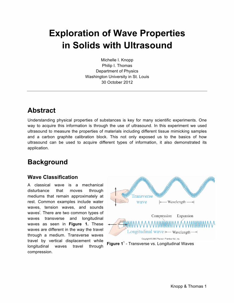
Wave Classification A classical wave is a mechanical disturbance that moves through mediums that remain approximately at rest. Common examples include water waves, tension waves, and sounds wavesi. There are two common types of waves transverse and longitudinal waves as seen in Figure 1. These waves are different in the way the travel through a medium. Transverse waves travel by vertical displacement while longitudinal waves travel through compression.
Figure 11 - Transverse vs. Longitudinal Waves
Knopp & Thomas 2
Acoustic Waves Sound waves, also known as acoustic waves, are fluctuations in the density of the medium described by a function in relationship to its equilibrium value. Ultrasound waves are a subset of acoustical waves with frequency over 20 kHz, typically less than 4-6 GHz, which exceeds the human hearing range. Acoustical waves require an elastic media to propagate because they result from the displacement of a position of an elastic medium from its normal position causing it to oscillate about an equilibrium position. Acoustic wave properties are affected by variables such as pressure, density, temperature and particle motion. ii These waves can transfer large amounts of energy in space by transmission of disturbance motion from one particle to another. Different kinds of acoustical waves are differentiated by their polarization, the motion of the particles of matter related to the direction of propagation of the wave itself. There are three modes of bulk waves possible one longitudinal (motion of particles is aligned with motion of waves) and two transverse waves (motion of particles is perpendicular to the motion of the waves). Fluids and gases can only support longitudinal propagation because they lack the restoring forces for shear deformations. The propagation speed is proportional to stiffness and inversely related to density.iii
Wave Interaction Waves exhibit many unique characteristics that are key to understanding the basic nature of how waves travel and interact with the environment and each other. The superposition model is the key to
understanding fundamental interference. This model states: if two waves are moving through a given medium, the function f(x,t) that describes the combined wave at any time t and any position x is simply the algebraic sum of the functions f1(x,t) and f2(x,t) that describe the individual waves: f(x,t)=f1(x,t)+f2(x,t). This phenomenon holds true due to the linearity of the waves.iv
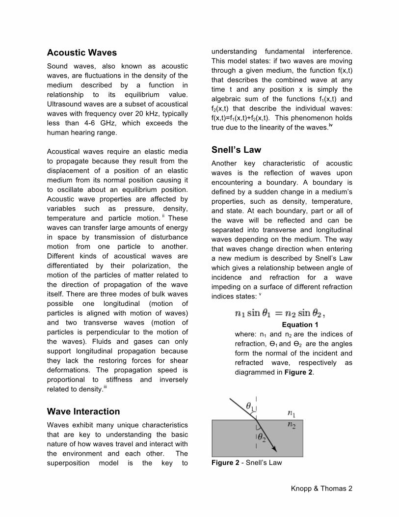
Snell’s Law Another key characteristic of acoustic waves is the reflection of waves upon encountering a boundary. A boundary is defined by a sudden change in a medium’s properties, such as density, temperature, and state. At each boundary, part or all of the wave will be reflected and can be separated into transverse and longitudinal waves depending on the medium. The way that waves change direction when entering a new medium is described by Snell’s Law which gives a relationship between angle of incidence and refraction for a wave impeding on a surface of different refraction indices states: v
Equation 1
where: n1 and n2 are the indices of refraction, ϴ1 and ϴ2 are the angles form the normal of the incident and refracted wave, respectively as diagrammed in Figure 2.
Figure 2 - Snell’s Law
Knopp & Thomas 3
Snell’s Law is derived from the Principle of Least Action which interprets Newton’s Second Law of Motion in Lagrangian mechanics by stating that the average kinetic energy less the average potential energy is as little as possible for the path of an object going from one point to another.vi This explains the changes in direction of waves as they interact over a boundary. Due to the differences of mediums at a boundary, waves become separated into different components. At the boundary between water and a plastic bar, the wave will split into longitudinal component and a transverse component. Due to the difference in the nature of these components they will travel with different velocities through the medium.
Propagation Velocity measurements seem very straightforward in principle. To find an average velocity one simple takes a measurement of the time it takes for a point to travel a certain displacement. This however assumes that this point is a part of an object whose structure does not change. Due to the interference of waves on a surface this cannot accurately be assumed for waves. For waves in the form of signals, a different technique is required. Different types of velocities such as phase velocity, group velocity, signal velocity, and wavefront velocity can be used to determine the velocity of the changing wave. A key characteristic of waves is its propagation through a medium. Just a friction in linear motion this results in a reduction of acoustic energy as the wave propagates through a medium. This is known as attenuation. This energy is
removed from the propagating wave by a variety of mediums such as absorption and scattering.
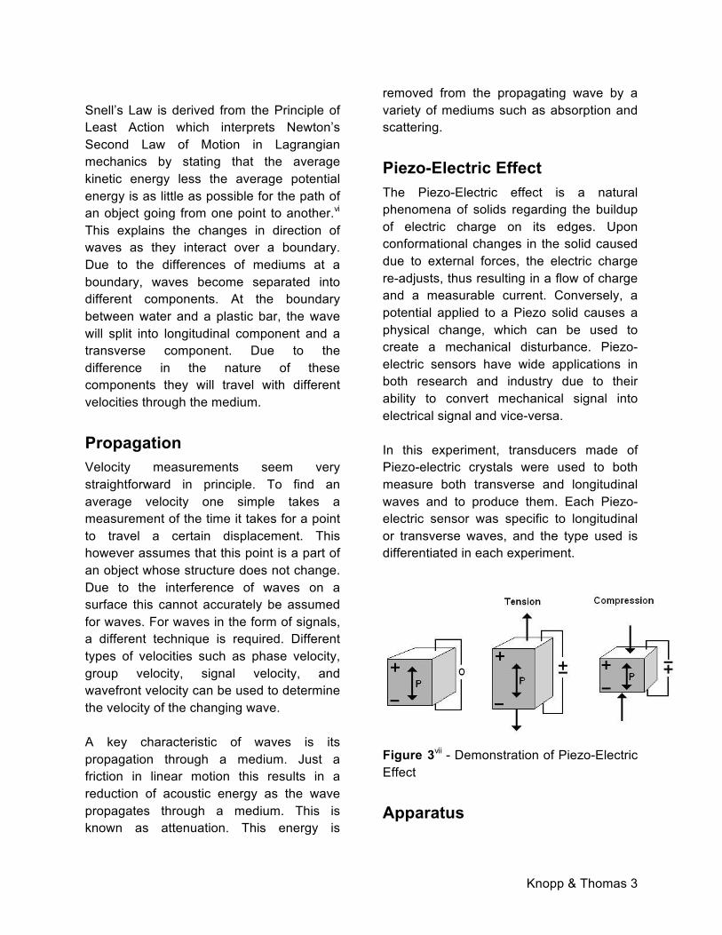
Piezo-Electric Effect The Piezo-Electric effect is a natural phenomena of solids regarding the buildup of electric charge on its edges. Upon conformational changes in the solid caused due to external forces, the electric charge re-adjusts, thus resulting in a flow of charge and a measurable current. Conversely, a potential applied to a Piezo solid causes a physical change, which can be used to create a mechanical disturbance. Piezo-electric sensors have wide applications in both research and industry due to their ability to convert mechanical signal into electrical signal and vice-versa. In this experiment, transducers made of Piezo-electric crystals were used to both measure both transverse and longitudinal waves and to produce them. Each Piezo-electric sensor was specific to longitudinal or transverse waves, and the type used is differentiated in each experiment.
Figure 3vii - Demonstration of Piezo-Electric Effect
Apparatus
Knopp & Thomas 4
Ultrasonic Pulse Receiver For this experiment we used the Metrotek MP215 to supply an electrical excitation pulse to the transmitting transducer, act as a clock to the purpose of accurate measurements, and use the MR101 receiver to provide gain to the received rf signal. For transmission the trigger unit generates a very narrow sharp negative going DC spike which causes the piezoelectric crystal in the transmitting transducer. This causes the crystal to vibrate which initiates a propagating pressure wave into the medium that the transducer is in contact with. For the reception of the signal the piezoelectric receiving transducer converts the pressure of the wave into an electrical representation of the radiofrequency wave. Since time is one of the key aspects of determining the velocity of these signals we depend on MP215 to act as a master clock and ensure proper sync between trigger and signal reception. It is possible to use this system in two different set-ups that allow for through-transmission and pulse/echo system. See Figure 9 for the wiring diagram that describes this diagram.
Oscilloscope We used a Tektronix 3000B series digital oscilloscope is used to display the received radiofrequency signal and to input this signal to the computer. The function of the oscilloscope has three basic modules: 1) vertical amplifier, 2) horizontal timing, and 3) triggering modules. The vertical scale has an 8-bit digitizer which means there are 28=256 discrete voltage levels each which has 25 levels per division. This is important because the vertical scale setting will affect
the sensitivity. The horizontal scale has ten horizontal divisions. The frequency of points depends on which mode is selected: 500 points for Fast Trig and 10,000 points for Normal. The time between each adjacent datum is:
Equation 2
where: number of points/div=record length/number of div. The oscilloscope allows us to display a delay of a fixed amount of time after the scope is triggered. This was instrumental to all our data acquisition.
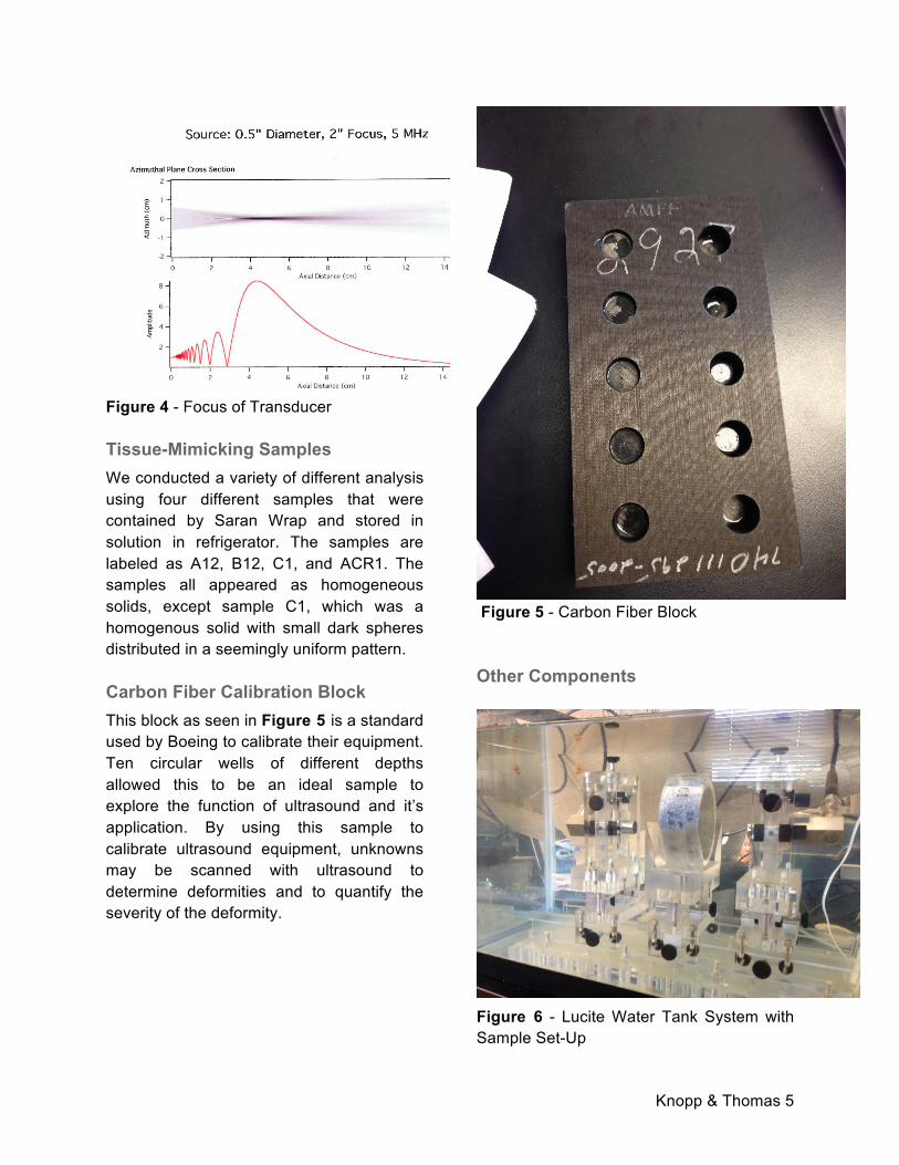
Transducers For most of this experiment we used two Panametric’s V309, .5” diameter, 2” point focal length, 5 MHz center-frequency longitudinal transducers. These transducers are manufactured to have a peak response at about 5 MHz and fall off on either side. These transducers are broadband which implies that the signal has a range of frequencies present simultaneously. This means that the usable frequency in water is 2-8 MHz. This equipment limitation is a limiting factor of results in the apparatus. These transducers were connected to the oscilloscope and pulse receiver using two BCU-58-6-W BNC to UHF waterproof cables.
Knopp & Thomas 5
Figure 4 - Focus of Transducer
Tissue-Mimicking Samples We conducted a variety of different analysis using four different samples that were contained by Saran Wrap and stored in solution in refrigerator. The samples are labeled as A12, B12, C1, and ACR1. The samples all appeared as homogeneous solids, except sample C1, which was a homogenous solid with small dark spheres distributed in a seemingly uniform pattern.
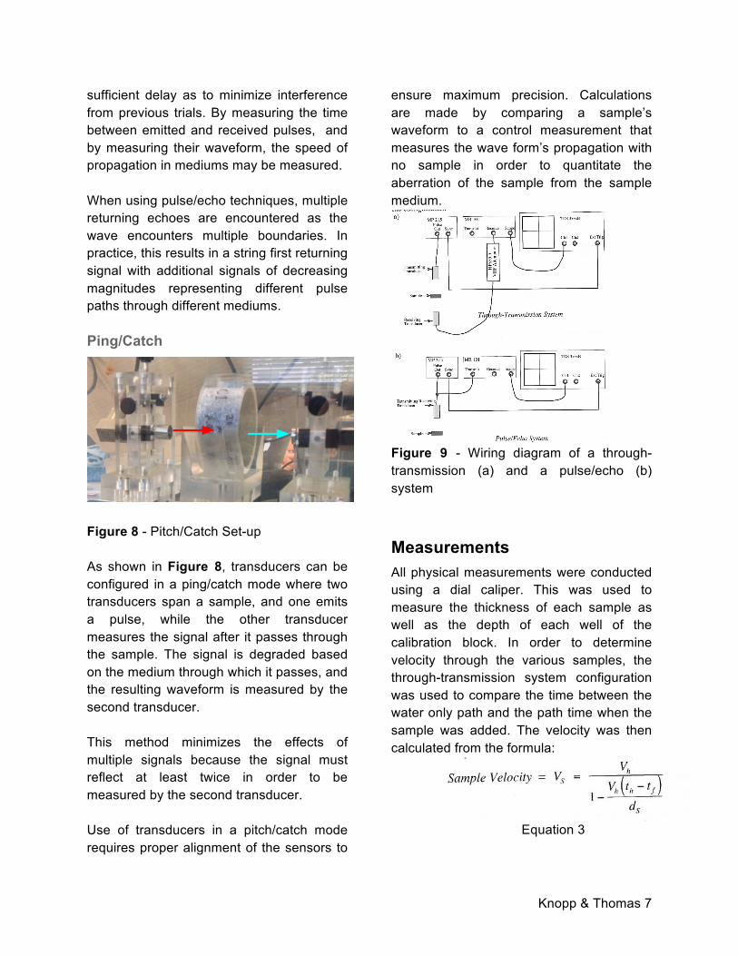
Carbon Fiber Calibration Block This block as seen in Figure 5 is a standard used by Boeing to calibrate their equipment. Ten circular wells of different depths allowed this to be an ideal sample to explore the function of ultrasound and it’s application. By using this sample to calibrate ultrasound equipment, unknowns may be scanned with ultrasound to determine deformities and to quantify the severity of the deformity.
Figure 5 - Carbon Fiber Block
Other Components
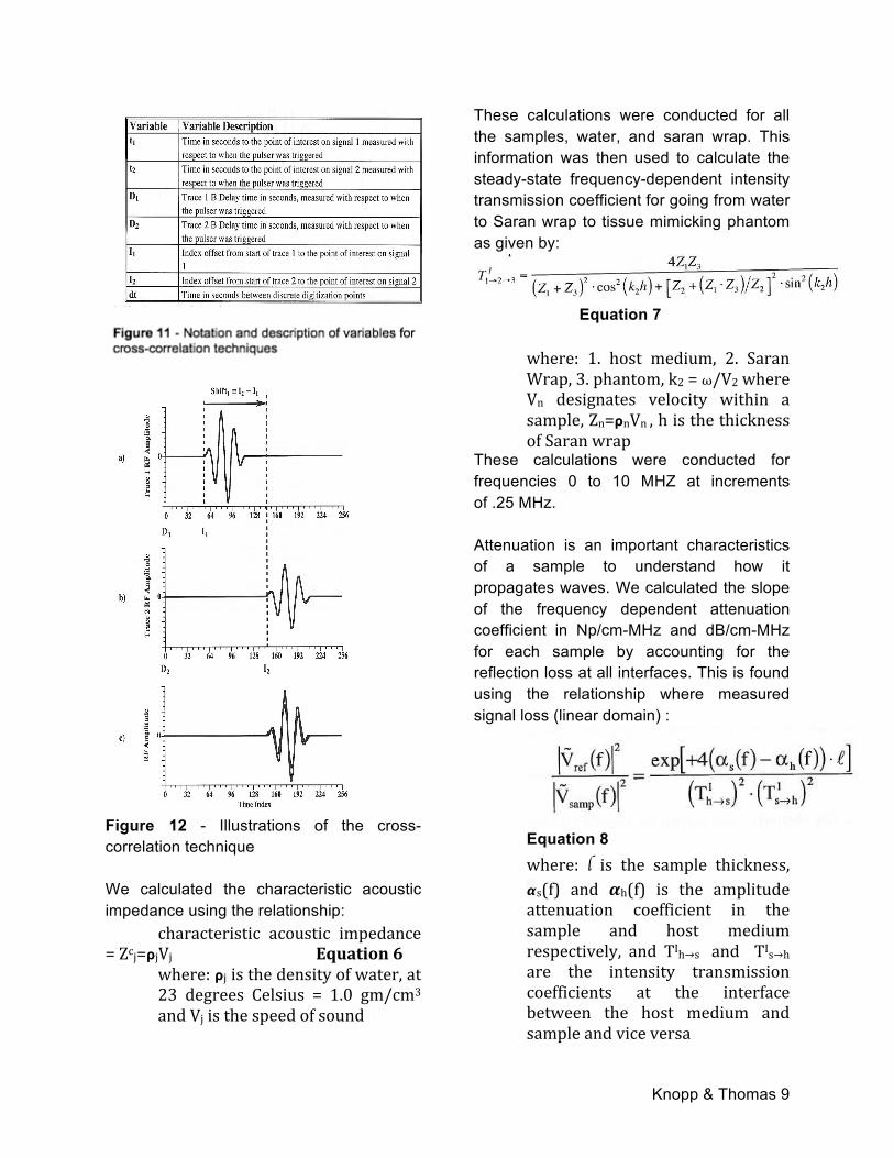
Figure 6 - Lucite Water Tank System with Sample Set-Up
Knopp & Thomas 6
See Figure 6 to see a diagram of the Lucite Water Tank System in which almost all experiments were conducted. This system holds the transducers in place in a larger water bath while allowing for two degrees of sample manipulation and five degrees of transducer manipulation: vertical movement, perpendicular horizontal movement, parallel horizontal movement, and pitch and yaw adjustment. Three 50 ohm RG-58 coaxial BNC cables were used to connect components. Two HP VHF Attenuators were used to increase the attenuation of the signal. The 355D adds up to 120 dB in 10 dB steps which the 355C adds up to 12 dB in 1 dB steps.
Methods/Procedure In this experiment we measured the longitudinal signal velocity, acoustic impedance, and frequency- dependent attenuation coefficient for four tissue-mimicking phantoms using ultrasound.
Alignment In order to obtain good data the transducer system must be properly aligned. Since the focal point of the transducer is two inches from the face, we aligned the transducer perpendicular to a stainless steel sample two inches away. Using the Pulse/Echo configuration and the delay option, the sensor was iteratively manipulated until a maximum signal was achieved. We used the temperature to determine the expected speed of sound in water and used that to calibrate the front of the steel plate to actually be two inches away. We adjusted the pitch and yaw until we achieved a power spectrum (Fourier Transform) that had a broad spectrum from 2 to 8 MHz, a smooth
spectrum with no bumps or cuts in this range, and the largest possible area under the curve since this is proportional to the energy. The range of the spectrum was determined by the hardware specifications of the transducers. This was repeated for the second transducer. Once this was done the system was rewired for align for through transmission and attempt to maximize the power spectrum as before by adjusting the receiving transducer. At this point it was important to check for system linearity. Using in house software known as DynamicRange we acquired the Fourier graph for a range of different decibels of attenuation controlled by the VHF Attenuator. This allowed us to determine for what range the system was linear. It is important that all of this analysis and alignment is conducted before any measurements are actually taken.
Ultrasound Testing Techniques
Pulse/Echo
Figure 7 - Pulse/Echo Set-up As demonstrated by Figure 7, Pulse/Echo mode utilizes one transducer to measure the properties of a material. This transducer first emits an ultrasound pulse of a known frequency. The same transducer then measure returning signals (“echoes”) caused by the reflection of the waves at boundaries. Subsequent pulses are set at a
Knopp & Thomas 7
sufficient delay as to minimize interference from previous trials. By measuring the time between emitted and received pulses, and by measuring their waveform, the speed of propagation in mediums may be measured. When using pulse/echo techniques, multiple returning echoes are encountered as the wave encounters multiple boundaries. In practice, this results in a string first returning signal with additional signals of decreasing magnitudes representing different pulse paths through different mediums.
Ping/Catch
Figure 8 - Pitch/Catch Set-up As shown in Figure 8, transducers can be configured in a ping/catch mode where two transducers span a sample, and one emits a pulse, while the other transducer measures the signal after it passes through the sample. The signal is degraded based on the medium through which it passes, and the resulting waveform is measured by the second transducer. This method minimizes the effects of multiple signals because the signal must reflect at least twice in order to be measured by the second transducer. Use of transducers in a pitch/catch mode requires proper alignment of the sensors to
ensure maximum precision. Calculations are made by comparing a sample’s waveform to a control measurement that measures the wave form’s propagation with no sample in order to quantitate the aberration of the sample from the sample medium.
Figure 9 - Wiring diagram of a through-transmission (a) and a pulse/echo (b) system
Measurements All physical measurements were conducted using a dial caliper. This was used to measure the thickness of each sample as well as the depth of each well of the calibration block. In order to determine velocity through the various samples, the through-transmission system configuration was used to compare the time between the water only path and the path time when the sample was added. The velocity was then calculated from the formula:
Equation 3
Knopp & Thomas 8
where: (th-tf) is the difference in time measured between water-path-only and with sample inserted, ds is thickness of the sample, and Vh is the velocity of the host material (in this case water, temperature dependent)
It is important to keep in mind that time between adjacent datum points is ∆t=time/div / number of points/div. The velocity of water is calculated here using a fifth order polynomial equation presented by Lovett as:
+3.0449*10-9T5 Equation 4viii where: T is degrees of water (oC) and Vh the velocity of water (m/s)
The time shift is calculated from a two step process of cross-correlation analysis. First, individual radio frequency waveforms are visually inspected to ensure quality and
maximum power spectrum. The second component uses computer analysis to determine the time shift needed to provide maximum overlap of the two signals of interest. This is done by symmetric cross-correlation technique in which:
Equation 5 where: tn=Dn+In dt, so that cross-correlation is the maximum overlap of the two traces as seen in Figure 12, other variables are defined in Figure 11.
Figure 10 - Velocity Measurement Geometry
Knopp & Thomas 9
Figure 12 - Illustrations of the cross-correlation technique We calculated the characteristic acoustic impedance using the relationship: characteristic acoustic impedance = Zcj=ρjVj Equation 6
where: ρj is the density of water, at 23 degrees Celsius = 1.0 gm/cm3 and Vj is the speed of sound
These calculations were conducted for all the samples, water, and saran wrap. This information was then used to calculate the steady-state frequency-dependent intensity transmission coefficient for going from water to Saran wrap to tissue mimicking phantom as given by:
Equation 7
where: 1. host medium, 2. Saran Wrap, 3. phantom, k2 = ω/V2 where Vn designates velocity within a sample, Zn=ρnVn , h is the thickness of Saran wrap
These calculations were conducted for frequencies 0 to 10 MHZ at increments of .25 MHz. Attenuation is an important characteristics of a sample to understand how it propagates waves. We calculated the slope of the frequency dependent attenuation coefficient in Np/cm-MHz and dB/cm-MHz for each sample by accounting for the reflection loss at all interfaces. This is found using the relationship where measured signal loss (linear domain) :
Equation 8
where: l is the sample thickness, 𝞪s(f) and 𝜶h(f) is the amplitude attenuation coefficient in the sample and host medium respectively, and TIh→s and TIs→h are the intensity transmission coefficients at the interface between the host medium and sample and vice versa
Knopp & Thomas 10
This allows us to calculate the frequency-dependent attenuation coefficient by compensating for the intensity transmission coefficient:
Equation 9 where: Ref[f]-‐Sample[f] is the time shift found from cross-‐correlation, T11→2→3 and T13→2→1 are the steady-‐state frequency-‐dependent intensity transmission coefficients and sample thickness is the thickness of the sample, and 𝞪dBsample[f] is the frequency-‐dependent attenuation coefficient
Depth Measurements We set out to measure the depths of the Carbon Fiber Calibration Block by using ultrasound in our water-filled apparatus. We accomplished this by two ways: Ping/catch and throughput. For the ping/catch technique, we aligned the diode with each hole of the block individually. Care was given to keep the face of the block a constant distance from
the diode. In addition, each hole was adjusted for maximum signal with the transducer, therefore indicating that it was perpendicular to the face of the transducer. A time shift between the measurement of each single hole relative to the solid face of the block was obtained. This time, multiplied by speed of sound in water, gave the round-trip distance that the sound traveled. By comparing the solid face distance to that of each hole, and by dividing by a factor of two to account for the time-shift measuring round-trip distance, the depth of each hole could be determined. A second measurement was taken using a throughput technique. Here, a water path between the transducers was used as a baseline, then the block is positioned between the transducers, perpendicular to the measured signal path. After aligning each hole using the same amplitude-maximization technique as the depth measurements, a path was recorded, then a time shift was calculated. By using the known thickness of the block with the full-width time shift, we were able to calculate the thickness of the carbon fiber at every single well on the block. Therefore, by subtracting that thickness from the total block thickness, the well depth was calculated.
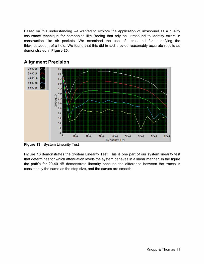
Results Overall this experiment allowed us to learn about ultrasonics and its different applications, calculations, and limitations. After aligning our system we learned about it was linear for a range of 20.00-40.00 dB. Linearity is demonstrated when the difference between the trace and the step size is the same. This is demonstrated for 20.00 to 40.00 dB range in Figure 13. We then successfully found the velocities of all the samples which revealed that the velocity was lowest in sample C1 which was not homogenous like the other samples. We successfully calculated the attenuation coefficient for all the samples and determined the best frequencies. All of this data acquisition allow us to gain a proper understand of the equipment and data analysis techniques.
Knopp & Thomas 11
Based on this understanding we wanted to explore the application of ultrasound as a quality assurance technique for companies like Boeing that rely on ultrasound to identify errors in construction like air pockets. We examined the use of ultrasound for identifying the thickness/depth of a hole. We found that this did in fact provide reasonably accurate results as demonstrated in Figure 20.
Alignment Precision
Figure 13 - System Linearity Test Figure 13 demonstrates the System Linearity Test. This is one part of our system linearity test that determines for which attenuation levels the system behaves in a linear manner. In the figure the path’s for 20-40 dB demonstrate linearity because the difference between the traces is consistently the same as the step size, and the curves are smooth.
Knopp & Thomas 12
Sample
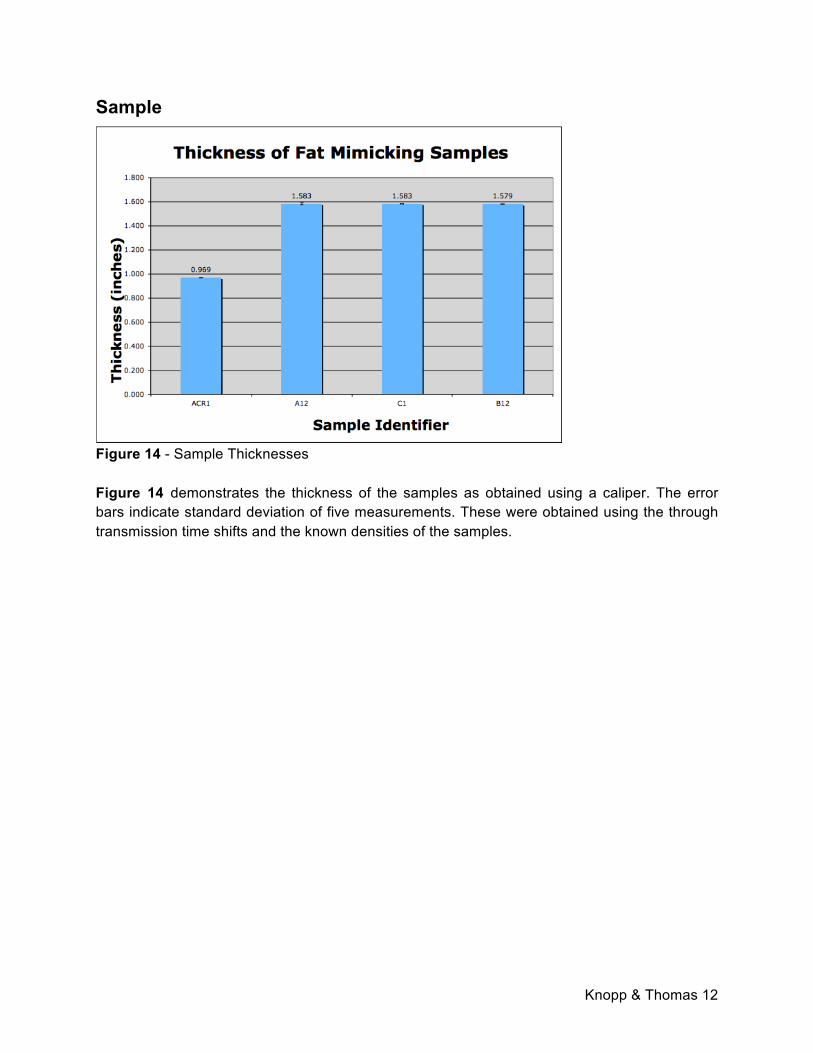
Figure 14 - Sample Thicknesses Figure 14 demonstrates the thickness of the samples as obtained using a caliper. The error bars indicate standard deviation of five measurements. These were obtained using the through transmission time shifts and the known densities of the samples.
Knopp & Thomas 13
Figure 15 - Velocities of Samples Figure 15 shows the velocity of sound in the samples as determined using ultrasound compared to water. These were calculated using a cross-correlation analysis and the thickness of the sample with comparison to the water-path. These are all dependent on temperature. The standard deviation is marked from the five different acquisitions acquired by rotating the sample.
Knopp & Thomas 14
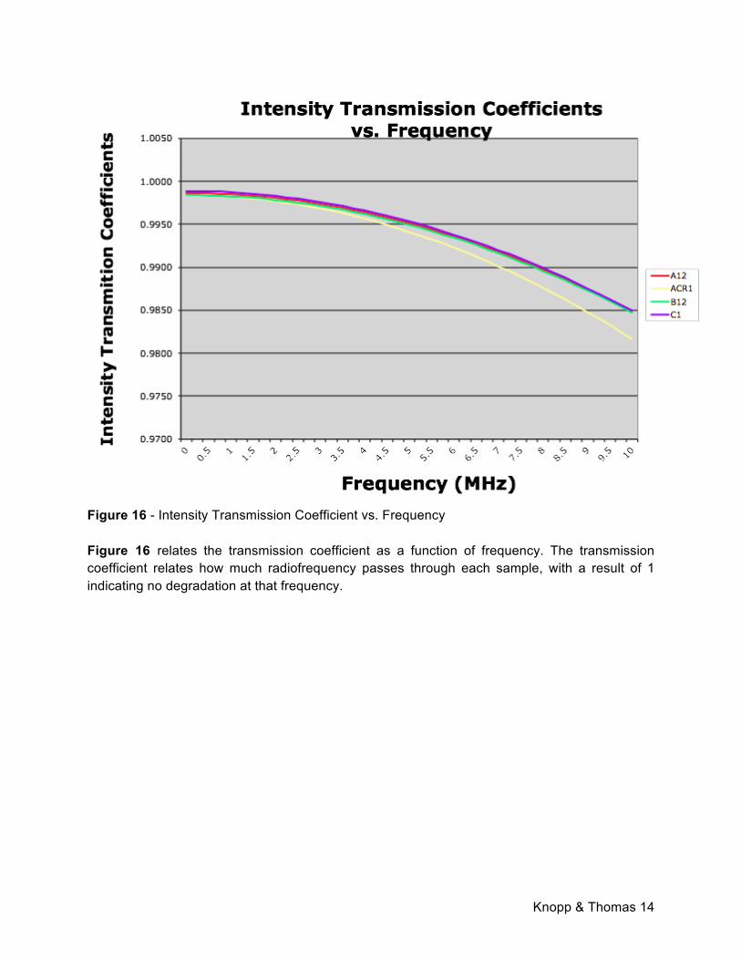
Figure 16 - Intensity Transmission Coefficient vs. Frequency Figure 16 relates the transmission coefficient as a function of frequency. The transmission coefficient relates how much radiofrequency passes through each sample, with a result of 1 indicating no degradation at that frequency.
Knopp & Thomas 15
Figure 17 - Graph of the Linear Attenuation Correction factor as calculated for all four tissue mimicking samples from the range that a linear relationship was found. This was found true for the ranges demonstrates in Figure 18. Sample Range (MHz) A12 1.5-6.5 ACR1 1-6 B12 1.25-5.5 C1 1.25-3.75 Figure 18 - Range of Frequency Used to Calculate Linear Fit: This table demonstrates the range over which the equation is Figure 17 were calculated from.
Knopp & Thomas 16
Calibration Block
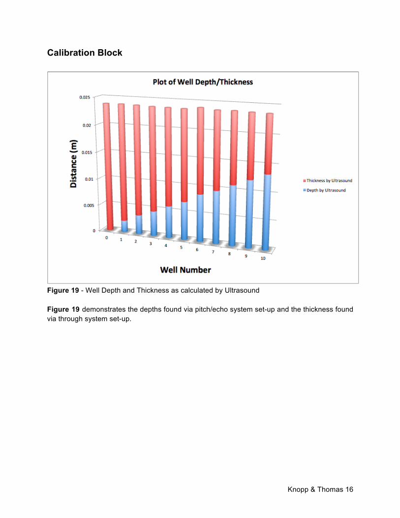
Figure 19 - Well Depth and Thickness as calculated by Ultrasound Figure 19 demonstrates the depths found via pitch/echo system set-up and the thickness found via through system set-up.
Knopp & Thomas 17
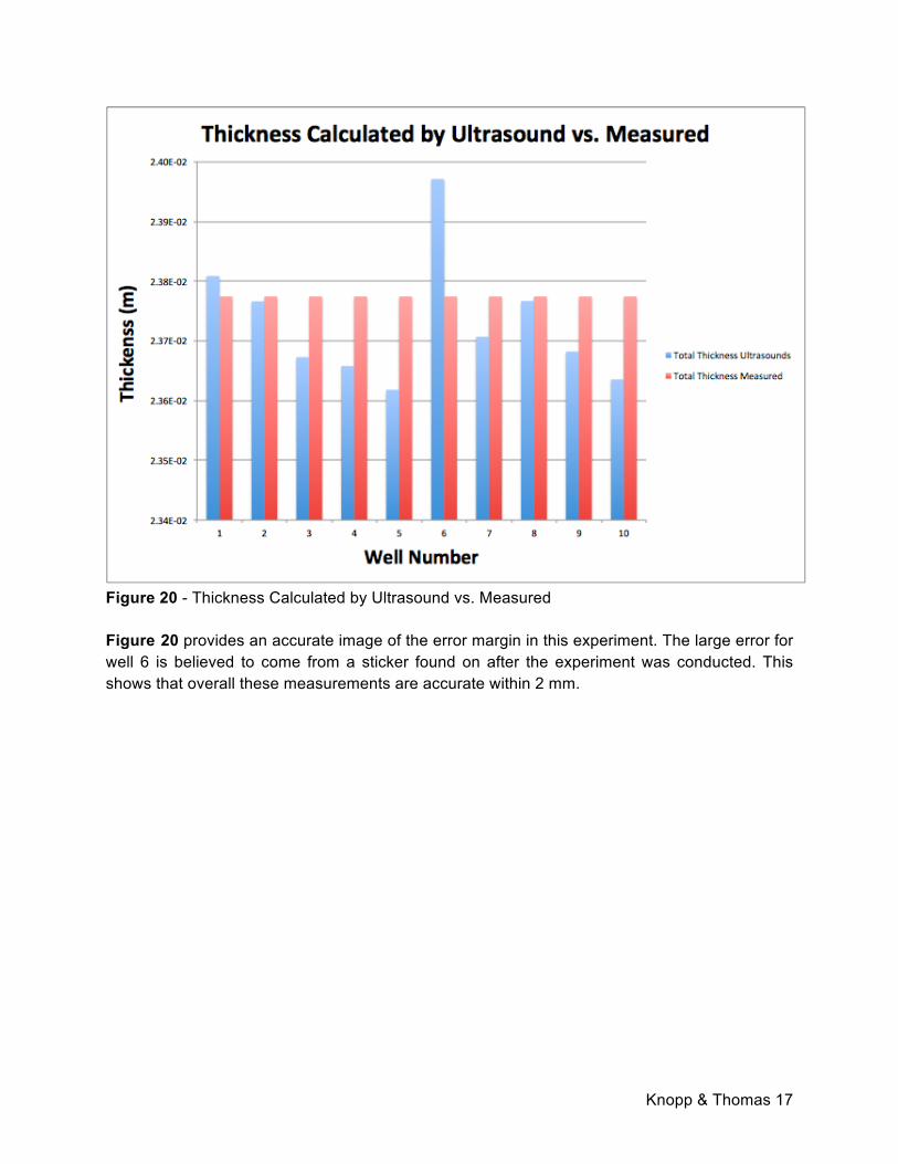
Figure 20 - Thickness Calculated by Ultrasound vs. Measured Figure 20 provides an accurate image of the error margin in this experiment. The large error for well 6 is believed to come from a sticker found on after the experiment was conducted. This shows that overall these measurements are accurate within 2 mm.
Knopp & Thomas 18
Discussion Ultrasound is typically used for qualitative data such as ultrasound images of fetal development. However, it is also used for quantitative analysis such as doppler to analyze blood flow in veins. We really enjoyed running a variety of different tests and to learn about the possible applications and limitations of this equipment. Based on Figure 13, we demonstrate that the system is linear for the range of 20-40 dB. The graph shows a smooth curve with consistent with linear systems. This allows us to conclude that the transducers are properly aligned for this range. Furthermore, we conclude that this range correlates with properties of the transducers due to the Piezo-electric effect and basic wave properties. Precise thickness measurement of the samples are a precursor to attaining precise velocity measurements. Figure 14 demonstrates that the samples are of uniform thickness. We can then conclude that the mean is sufficiently precise for use in further analysis. We expect the speed of sound in tissue to be comparable to that of water due to the high water content within tissue. Hence, the sample velocities obtained in Figure 15 are all in a range consistent with this hypothesis. The method of calculation in Equation 7 proved important because of the high velocity of sound in the encasing saran wrap, which causes high reflection and must be accounted for.
The intensity transmission coefficient shows that, for all samples, reflection increases as frequency increases. This is consistent with our understanding of ultrasound in water and water-based mediums, where signal degrades as frequency increases. Intuitively, this is why SONAR navigation uses audible mid-frequency sound waves to obtain a precision reading at distance using sound underwater. ix Figure 17 demonstrates that frequency increases correlate to attenuation correction. This conclusion is reasonable because higher frequency waves have higher energy, and hence signal degradation in an elastic medium is expected to correlate with frequency. In addition, the linear region of this graph falls within the specification range of the transducer. Furthermore, the high attenuation correction for sample C1 may be attributed to its non-homogenous medium. As the wave passes through the sample, inhomogeneities cause additional reflection and energy loss. This leads both to the higher slope of the line and the more narrow linear frequency region. Upon understanding the basics of ultrasound, we became interested in its industrial application. We therefore designed and conducted an experiment which successfully tested the depth of various wells in a standard carbon graphite calibration block. This has many exciting applications in manufacturing by providing quantifiable metrics for quality assurance. Specifically, the wavelength of ultrasound, coupled with its safety and accessibility, allows for accurate measurements of material properties that can be used to identify errors or inconsistencies. Specifically with the block used in our experiment, calibrations with the properties
Knopp & Thomas 19
of carbon fiber-based materials allows for the detection of errors in the manufacturing process, such as errant plastic or air bubbles which could threaten the structural integrity of the product. Our measurements demonstrate the precision of ultrasound for measuring sample uniformity. Specifically, the throughput method of determining the thickness of the material provided a metric with precision that would allow for the detection of anomalies in the material plus an confidence interval for the quantification of the likelihood of error. The accuracy of our measurements was in general within two millimeters of the measured thickness. One anomaly existed on the rear of the block, in the form of metallic sticker roughly 3mm in diameter. The decreased precision well 6 as demonstrated in Figure 20 may be attributed to this nonuniformity. Overall these were found to add up to be surprisingly similar to the actual thickness of the entire block. This demonstrates the feasibility of using ultrasound to test for irregularities.
Experimental Error While everything was done to limit experimental error, ultimately it is impossible to avoid. Some came about from our procedure while others are limitations of our equipment. Due to the time constraint in our lab set-up we were also limited by our understand of the equipment and the lack of time to fully test all parameters to understand the impact of various conditions. By examining the properties of the four tissue-mimicking samples we were able to
gain a decent understanding about the difference in velocity and attenuation. This helped us learn about the basic formulas and laws of physics play out behind our results. One factor that we only have limited control over was temperature. Although we conducted all scans that were compared to each other as quickly as possible at the same time point. Due to our hands being in the water tank to switch and hold the sample, the water bath temperature slightly increased during scans. We did our best to equilibrate our samples to the temperature of the water bath from the refrigerator by placing the samples in the water for approximately an hour. While we did our best to double check our results and make sure everything is reasonable it is possible that there are errors in our equations. We also needed to do a lot of conversions between inches and meters due to the measuring equipment we had access too. While all these calculations results seem reasonable there is always a possibility of error. The alignment of the transducers was determined to be of reasonable precision on the initial day of experimentation. However, as the apparatus was used in the following two weeks, it is possible that the alignment changed. With the constant agitation in the water bath and manipulation of samples on the rig, it is reasonable to assume that the alignment changed slightly. However, no inconsistencies appeared over the time period of the experiment to signal that alignment had beyond acceptable error. In addition, care was taken to not touch the transducers in order to keep the alignment as undisturbed as possible.
Knopp & Thomas 20
While the velocity sound in water as a function of temperature is a known, we were unable to control the purity of the water. Soluble substances such as salts and gases may have changed the velocity of sound and may have altered the diffraction of sound in the water. Initially, tap water was used to fill the tank, and bleach was intentionally added to prevent the growth of fungi Over the time period of the trials, it became obvious due to the smell and appearance of the water that some unknown growth was occurring in the water. As we manipulated the samples in the water, impurities were introduced by our hands. The samples themselves introduced impurities to the water. Overall, literature statesx that the speed of sound in water “[ . . . ] very sensitive to impurities.” Because we were unable to directly measure the speed of sound in a given sample of water, we conducted trials sequentially, thus minimizing the time of each experiment and allowing us to approximate the level of purity of the water as constant during the course of each experiment. The equipment was imperfect; specifically, the Piezo crystals are not ideal. In addition, ambient magnetic fields plus imperfections in the wires likely caused imperfect signal transmission.
Conclusion After examining our results, we are encouraged by the industrial applications of ultrasound. In future experimentation we seek to study known inhomogeneities in a sample to understand the precision and accuracy of ultrasound for determining size, dimension, and location. We enjoyed the opportunity to explore the application of ultrasound in this setting.
Knopp & Thomas 21
Sources i Moore, Thomas A. "Standing Waves." Six Ideas That Shaped Physics - Unit Q: Particles Behave Like Waves. Second ed. St. Louis: McGraw Hill, 2003. 2-17. Print. ii Kremkau, Frederick W. Diagnostic Ultrasound Principles and Instruments. Fourth ed. Philadelphia: W.B.Saunders, n.d. Print. iii Kremkau, Frederick W. Diagnostic Ultrasound Principles and Instruments. Fourth ed. Philadelphia: W.B.Saunders, n.d. Print iv Moore, Thomas A. "Standing Waves." Six Ideas That Shaped Physics - Unit Q: Particles Behave Like Waves. Second ed. St. Louis: McGraw Hill, 2003. 2-17. Print. v Weisstein, Eric W. "Snell's Law." Snell's Law -- from Eric Weisstein's World of Physics. Wolfram Research, 2007. Web. 23 Oct. 2012. <http://scienceworld.wolfram.com/physics/SnellsLaw.html>. vi Leighton, Robert B., and Matthew Sands. "The Principle of Least Action." The Feynman Lectures of Physics - Mainly Electromagnetism and Matter. By Richard P. Feynman. Reading, MA: Addison-Wesley Coompany, n.d. 19-1-9-7. Print. vii "Piezoelectric-based Energy Harvesting." Piezoelectric-based Energy Harvesting. Stevens Institute of Technology, n.d. Web. 28 Oct. 2012. <http://www.ece.stevens-tech.edu/sd/archive/07F-08S/websites/grp3/piezoelectric.html>. viii Lovett, J. R. "Comments Concerning the Determination of Absolute Sound Speeds in Distilled and Seawater and Pacific Sofar Speeds." The Journal of the Acoustical Society of America 45.4 (1969): 1051. Print. ix Elert, Glen. "Frequency Used In Navigational Sonar." Frequency Used In Navigational Sonar. The Physics Factbook, n.d. Web. 30 Oct. 2012. <http://hypertextbook.com/facts/2001/EmranYusufov.shtml>. x http://thermosymposium.nist.gov/archive/symp17/pdf/Abstract_404.pdf