Exploring selﬁsh reinforcement learning in … Agent Multi-Agent Syst DOI...

Auton Agent Multi-Agent SystDOI 10.1007/s10458-006-9007-0

Exploring selfish reinforcement learning in repeatedgames with stochastic rewards

Katja Verbeeck · Ann Nowé · Johan Parent ·Karl Tuyls

Springer Science+Business Media, LLC 2006

Abstract In this paper we introduce a new multi-agent reinforcement learning algo-rithm, called exploring selfish reinforcement learning (ESRL). ESRL allows agentsto reach optimal solutions in repeated non-zero sum games with stochastic rewards,by using coordinated exploration. First, two ESRL algorithms for respectively com-mon interest and conflicting interest games are presented. Both ESRL algorithms arebased on the same idea, i.e. an agent explores by temporarily excluding some of thelocal actions from its private action space, to give the team of agents the opportunityto look for better solutions in a reduced joint action space. In a latter stage these twoalgorithms are transformed into one generic algorithm which does not assume that thetype of the game is known in advance. ESRL is able to find the Pareto optimal solu-tion in common interest games without communication. In conflicting interest gamesESRL only needs limited communication to learn a fair periodical policy, resulting ina good overall policy. Important to know is that ESRL agents are independent in thesense that they only use their own action choices and rewards to base their decisionson, that ESRL agents are flexible in learning different solution concepts and they canhandle both stochastic, possible delayed rewards and asynchronous action selection.A real-life experiment, i.e. adaptive load-balancing of parallel applications is added.

K. Verbeeck (B)Computational Modeling Lab (COMO), Vrije Universiteit Brussel, Brussels, Belgiume-mail: [email protected]

A. NowéComputational Modeling Lab (COMO), Vrije Universiteit Brussel, Brussels, Belgiume-mail: [email protected]

J. ParentComputational Modeling Lab (COMO), Vrije Universiteit Brussel, Brussels, Belgiume-mail: [email protected]

K. TuylsInstitute for Knowledge and Agent Technology (IKAT), University of Maastricht,The Netherlands,e-mail: [email protected]

Auton Agent Multi-Agent Syst

Keywords Multi-agent reinforcement learning · Learning automata · Non-zero sumgames

1 Introduction

Exploring selfish reinforcement learning (ESRL) is a new approach to multi-agentreinforcement learning (MARL). It originates from the theory of learning automata(LA), an early version of reinforcement learning (RL), which has its roots in psychol-ogy [15]. The collective behavior of LA is one of the first examples of MARL thathave been studied. A learning automaton describes the internal state of an agent asa probability distribution over actions. These probabilities are adjusted based on thesuccess or failure of the actions taken. The work of [15] analytically treats learning notonly in the single automaton case, but also in the case of hierarchies and distributedinterconnections. Of special interest to MARL research is the work done within theframework of learning automata games.

Learning automata games were developed for learning repeated normal formgames, well known in game theory [18,6]. A central solution concept for these games,is that of a Nash equilibrium. Learning automata games with suitable reinforcementupdate schemes were proved to converge to one of the Nash equilibria in repeatedgames, [20,15]. However, global optimality is not guaranteed. As will be discussedlater, the same criticism holds for most work in current MARL research.

One important problem is that games can have multiple Nash equilibria and thusthe question arises which equilibrium the agents should learn. Another related issue,is how the rewards are distributed between the agents. In some systems, the overallperformance can only be as good as that of the worst performing agent. As such theagents have to learn to equalize the average reward they receive. A Nash equilibriumis not always fair in the sense that the agents’ rewards or payoffs are not necessarilydivided equally among them. Even worse, a Nash equilibrium can be dominated bya Pareto optimal solution which gives a higher payoff to all agents. So, in gameswith multiple equilibria, typically the agents have preferences toward different Nashequilibria.

In order to deal with the observations stated above, ESRL approaches not only theset of Nash equilibria, but also the set of Pareto Optimal solutions of the game. Assuch, the solution that is most suitable for the problem at hand can be selected. Forexample, an appropriate solution could be to learn what we call a periodical policy. Ina periodical policy, agents alternate between periods in which they play different pureNash equilibria, each equilibrium is preferred by one of the agents. As such, a fairsolution can be obtained for all agents in a game with conflicting interests. Note thatwe use the word fair in the sense that the solution will distribute the rewards equallyamong all agents. We call a solution optimally fair when there is no other solutionthat is also fair for the agents but gives the agents more reward on average. Periodicalpolicies were first introduced in [17].

The key feature of ESRL agents is that they use a form of coordinated explorationto reach the optimal solution in a game. ESRL is able to find attractors of the singlestage game in the same way a game of learning automata does. But, as soon as anattractor is visited, learning must continue in a subaction space from which that attrac-tor is removed. As such the team of agents gets the opportunity to look for possiblybetter solutions in a reduced space. So, ESRL searches in the joint action space of


the agents for attractors as efficiently as possible by shrinking it temporarily duringdifferent periods of play.

ESRL learning is organized in phases. Phases in which agents act independentlyand behave as selfish optimizers are alternated with phases in which agents are social,and act so as to optimize the group objective. The former phases are called explora-tion phases, while the latter phases are called synchronization phases. During thesesynchronization phases, attractors are removed from the joint action space by lettingeach agent remove one action from its private action space. For these synchronizationphases, limited communication may be necessary, however sometimes a basic signalsuffices. The name exploring selfish reinforcement learning stresses that during theexploration phases the agents behave as selfish reinforcement learners.

ESRL agents experience games either as a pure common interest game or as a con-flicting interest game. The expected rewards given in the game matrices we considerhere, represent the mean of a binomial distribution. Extensions to other continuousvalues distributions will discussed at the end. A nice property of ESRL agents is thatthey do not need to know in advance the type of the game. Also, no further restrictionsare imposed on the form of the game, for instance pure Nash equilibria may or maynot exist. In a common interest game, ESRL is able to find one of the Pareto optimalsolutions of the game. In a conflicting interest game, we show that ESRL agents learnoptimal fair, possibly periodical policies [17,26]. Important to know is that ESRLagents are independent in the sense that they only use their own action choices andrewards to base their decisions on, that ESRL agents are flexible in learning differ-ent solution concepts and they can handle both stochastic, possible delayed rewardsand asynchronous action selection. In [26] a job scheduling experiment is solved byconflicting interest ESRL agents. In this paper, we describe the problem of adaptiveload-balancing parallel applications, handled by ESRL agents as a common interestgame.

This paper is organized as follows. In the next section game theoretic terminologyis introduced. We continue with a short overview of learning automata theory inSect. 3. Next, ESRL in respectively stochastic common interest (Sect. 4) and con-flicting interest games (Sect. 5) is discussed. Testbed games are described and thebehavior of ESRL is analyzed. In Sect. 6, ESRL is generalized to stochastic non-zerosum games. In Sect. 7, the robustness of ESRL to delayed rewards and asynchronousaction selection is illustrated with the problem of adaptive load-balancing parallelapplications. Finally the last section discusses the work presented and summarizesrelated literature.

2 Game theoretic background

In this section we introduce game theoretic terminology of strategic normal formgames, see [18] for a detailed overview.

Assume a collection of n agents where each agent i has an individual finite set ofactions Ai. The number of actions in Ai is denoted by |Ai|. The agents repeatedlyplay a single stage game in which each agent i independently selects an individualaction a from its private action set Ai. The combination of actions of all agents atany time-step, constitute a joint action or action profile

→a from the joint action set

A = A1 × · · · × An. A joint action→a is thus a vector in the joint action space A, with

components ai ∈ Ai, i : 1 . . . n.


a21 a22

a11 (1,−1)

(1,−1)

(−1,1)

(−1,1)a12

Fig. 1 The Matching Pennies game: 2 children independently choose which side of a coin to show tothe other. If they both show the same side, the first child wins, otherwise child 2 wins

With each joint action→a ∈ A and agent i a distribution over possible rewards is

associated, i.e. ri : A → IR denotes agent i’s expected payoff or expected rewardfunction. The payoff function is often called the utility function of the agent, it rep-resents the preference relation each agent has on the set of action profiles. The tuple(n, A, r1...n) defines a single stage strategic game, also called a normal form game.

Usually 2 player strategic games are presented in a matrix, an example is givenin Fig. 1 and following. A row player, i.e. agent 1 and column player, i.e. agent 2are assumed. The rows and columns represent the actions for respectively the rowand column player. In the matrix the (expected) rewards for every joint action canbe found; the first(second) number in the table cell is the (expected) reward for therow(column) player.

The agents are said to be in a Nash equilibrium, when it is the case that no agentcan increase its own reward by changing its strategy when all the other agents stickto their equilibrium strategy. So, there is no incentive for the agents to play anotherstrategy than their Nash equilibrium strategy. Nash proved the following importantexistence result [16]:

Theorem 1 Every strategic game, which has finitely many actions has at least one mixedNash equilibrium.

Despite the existence theorem above, describing an optimal solution for strategicgames is not always easy. For instance an equilibrium point is not necessarily uniqueand when more than one equilibrium point exists they do not necessarily give the sameutility to the players. Even more, an equilibrium point does not take into account therelation between individual and group rationality.

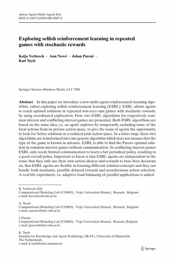
Pareto optimality is a concept introduced to account for group rationality. An out-come of a game is said to be Pareto optimal if there exists no other outcome, forwhich all players simultaneously perform better. The classical example of a situationwhere individually rationality leads to inferior results for each agent, is the Prisonner’sDilemma game, see Fig. 2. This game has just one Nash equilibrium which is pure i.e.joint action (a12, a22). However, it is the only pure strategy that is not Pareto opti-mal. Joint action (a11, a21) is obviously superior; it is the only strategy which Paretodominates the Nash equilibrium, however it is not a Nash equilibrium itself.

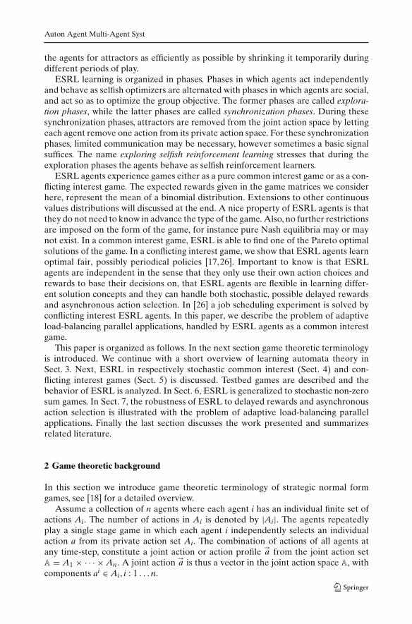
A special situation occurs when the individual utility of the agents coincides withthe joint utility of the group. These games are called common interest games. Incommon interest games the agents’ rewards are drawn from the same distribution.As a consequence, at least one Pareto optimal Nash equilibrium exists in commoninterest games and the agents’ learning objective is to coordinate on one of them. Allidentical payoff games, i.e. games that always give identical payoffs to all the agents,are common interest games. Figure 3 shows two examples of identical payoff games,that are non-trivial from a coordination point of view.


a21 a22

a11 (5,5)

a12 (10,0) (1,1)

(0,10)

Fig. 2 The Prisoner’s Dilemma Game: 2 prisoners committed a crime together. They can eitherconfess their crime (i.e. play the first action) or deny it (i.e. play the second action). When only oneprisoner confesses, he takes all the blame for the crime and receives no reward, while the other onegets the maximum reward of 10. When they both confess a reward of 5 is received, otherwise theyonly get 1

a21 a22 a23a11 11

70 0 5

630

300−

a12 −a13

a21 a22 a23a11 10

10

0

00 02

k

a12a13 k

Fig. 3 Left: The climbing game, an identical payoff game from [4]. The Pareto optimal Nash equilib-rium (a11, a21) is surrounded by heavy penalties. Right: The penalty game, an identical payoff gamefrom [4]. Mis-coordination at the Pareto optimal Nash equilibria (a11, a21) and (a13, a23) is penalizedwith k

a21 a22

a11 (2,1)

(1, 2)

0)

a12

(0,

0)(0,

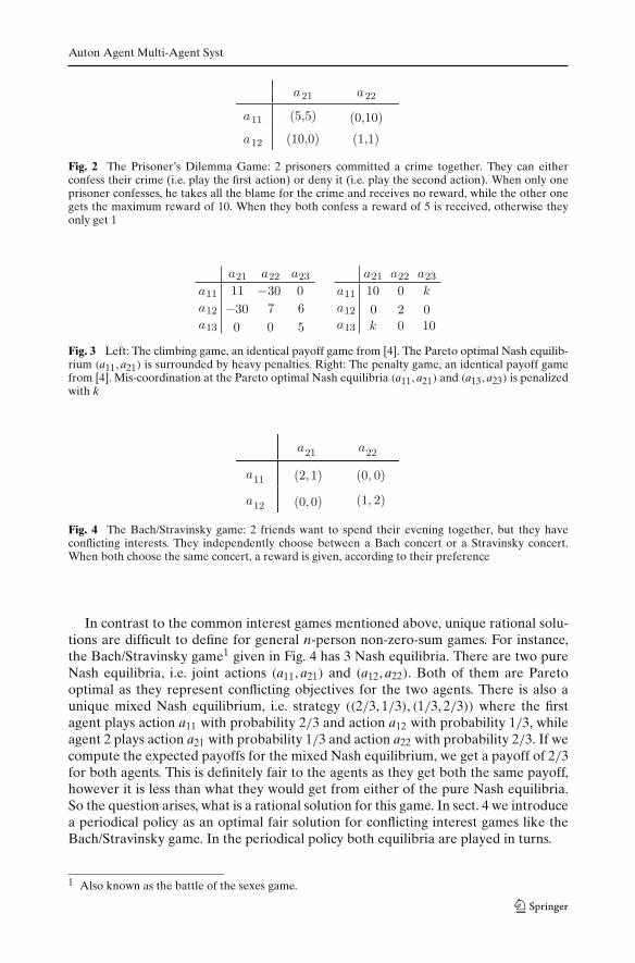
Fig. 4 The Bach/Stravinsky game: 2 friends want to spend their evening together, but they haveconflicting interests. They independently choose between a Bach concert or a Stravinsky concert.When both choose the same concert, a reward is given, according to their preference

In contrast to the common interest games mentioned above, unique rational solu-tions are difficult to define for general n-person non-zero-sum games. For instance,the Bach/Stravinsky game1 given in Fig. 4 has 3 Nash equilibria. There are two pureNash equilibria, i.e. joint actions (a11, a21) and (a12, a22). Both of them are Paretooptimal as they represent conflicting objectives for the two agents. There is also aunique mixed Nash equilibrium, i.e. strategy ((2/3, 1/3), (1/3, 2/3)) where the firstagent plays action a11 with probability 2/3 and action a12 with probability 1/3, whileagent 2 plays action a21 with probability 1/3 and action a22 with probability 2/3. If wecompute the expected payoffs for the mixed Nash equilibrium, we get a payoff of 2/3for both agents. This is definitely fair to the agents as they get both the same payoff,however it is less than what they would get from either of the pure Nash equilibria.So the question arises, what is a rational solution for this game. In sect. 4 we introducea periodical policy as an optimal fair solution for conflicting interest games like theBach/Stravinsky game. In the periodical policy both equilibria are played in turns.

1 Also known as the battle of the sexes game.


3 Learning automata

ESRL agents are simple reinforcement learners, more in particular they use a learningautomata update scheme. In this section we give an overview of learning automatatheory, in which we focus on automata games.

A learning automaton formalizes a general stochastic system in terms of states,actions, state or action probabilities and environment responses, see [15,22]. A learn-ing automaton is a precursor of a policy iteration type of reinforcement learningalgorithm [21] and has some roots in psychology and operations research. The designobjective of an automaton is to guide the action selection at any stage by past actionsand environment responses, so that some overall performance function is improved.At each stage the automaton chooses a specific action from its finite action set andthe environment provides a random response.

In its current form, a learning automaton updates the probabilities of its variousactions on the basis of the information the environment provides. Action probabilitiesare updated at every stage using a reinforcement scheme T.

Definition 1 A stochastic learning automaton is a quadruple {A, β, p, T} for which Ais the action set of the automaton, β is a random variable in the interval [0, 1] anddenotes the environment response, p is the action probability vector of the automatonand T denotes the update scheme.

A linear update scheme that behaves well in a wide range of settings2 is the linearreward-inaction scheme, denoted by (LR-I). The philosophy of this scheme is essen-tially to increase the probability of an action when it results in a success and to ignoreit when the response is a failure. The update scheme is given by:

Definition 2 The linear reward-inaction update scheme for binary environment re-sponses updates the action probabilities as follows: given that action ai is chosen attime t then if action ai was successful:

pi(t + 1) = pi(t)+ α(1− pi(t))

for action ai

pj(t + 1) = pj(t)− αpj(t)

for all actions aj �= ai

Otherwise when action ai failed, nothing happens.

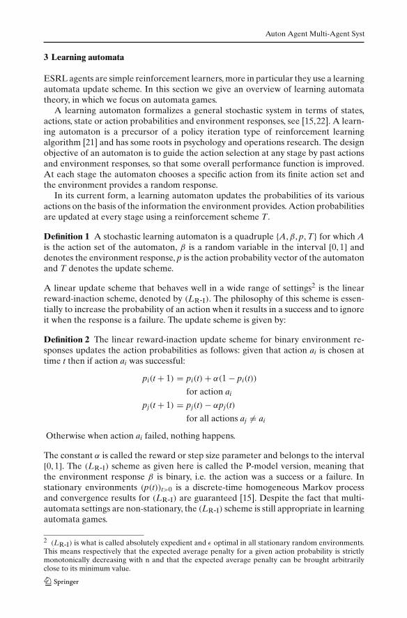
The constant α is called the reward or step size parameter and belongs to the interval[0, 1]. The (LR-I) scheme as given here is called the P-model version, meaning thatthe environment response β is binary, i.e. the action was a success or a failure. Instationary environments (p(t))t>0 is a discrete-time homogeneous Markov processand convergence results for (LR-I) are guaranteed [15]. Despite the fact that multi-automata settings are non-stationary, the (LR-I) scheme is still appropriate in learningautomata games.

2 (LR-I) is what is called absolutely expedient and ε optimal in all stationary random environments.This means respectively that the expected average penalty for a given action probability is strictlymonotonically decreasing with n and that the expected average penalty can be brought arbitrarilyclose to its minimum value.


A1

An

. . .

Environment

α β

β1α1

p1

pn

nn

...

Fig. 5 Automata game formulation

3.1 Learning automata games

Automata games were introduced to see if automata could be interconnected in use-ful ways so as to exhibit group behavior that is attractive for either modeling orcontrolling complex systems.

A play→a(t) of n automata is a set of strategies chosen by the automata at stage t,

such that aj(t) is an element of the action set of the jth automaton. Correspondingly theoutcome is now also a vector β(t) = (β1(t) · · ·βn(t)). At every time-step all automataupdate their probability distributions based on the responses of the environment.Each automaton participating in the game operates without information concerningthe number of other participants, their strategies, actions or payoffs (See Fig. 5).

The following results were tested and proved in [15]: In identical payoff games aswell as some non-zero-sum games it is shown that when the automata use a (LR-I)

scheme the overall performance improves monotonically. Moreover if the identicalpayoff game is such that a unique, pure Nash equilibrium point exists, convergenceis guaranteed. In cases were the game matrix has more than one pure equilibriumthe (LR-I) scheme will converge to one of the Nash equilibria. Which equilibrium isreached depends on the initial conditions.

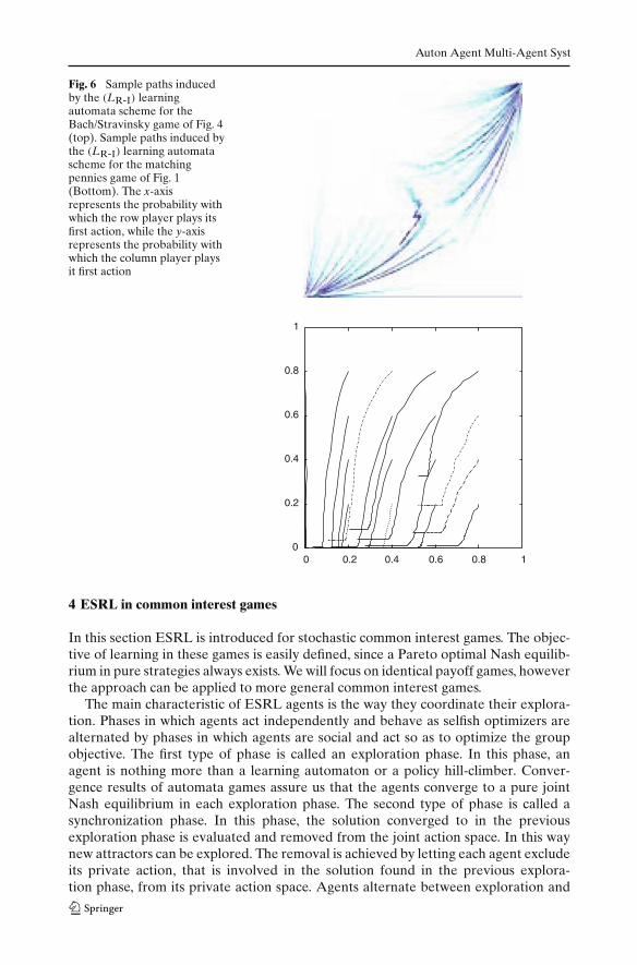
In [24] the dynamics of several reinforcement learning algorithms (including the(LR-I) scheme) is studied by mapping the algorithms into the replicator dynamicsfrom evolutionary game theory, [19]. Paths with different starting points induced bythe learning process of the (LR-I) scheme are visualized in Fig. 6 for respectively theBach/Stravinsky game of Fig. 4 and the matching pennies game of Fig. 1. The agents’probabilities of playing the first action are plotted against each other. In the first gametwo pure Nash equilibria exist, and the (LR-I) agents are able to find them. Whichequilibrium is reached depends on the initialization of the agent’s action probabilities.The last game has only one mixed equilibrium, in this case the agents converge to apure joint action, which is not Nash. In general for the (LR-I) scheme, the followingcan be proved [25].

Lemma 1 With probability 1 a team of LR-I learning automata will always converge toa limit in which all players play some pure strategy.

An important issue here is the dependence of the convergence on the size of thestep-size α. As shown in the following sections learning automata games of (LR-I)

schemes will form the basis for ESRL.


Fig. 6 Sample paths inducedby the (LR-I) learningautomata scheme for theBach/Stravinsky game of Fig. 4(top). Sample paths induced bythe (LR-I) learning automatascheme for the matchingpennies game of Fig. 1(Bottom). The x-axisrepresents the probability withwhich the row player plays itsfirst action, while the y-axisrepresents the probability withwhich the column player playsit first action

0

0.2

0.4

0.6

0.8

1

0 0.2 0.4 0.6 0.8 1

4 ESRL in common interest games

In this section ESRL is introduced for stochastic common interest games. The objec-tive of learning in these games is easily defined, since a Pareto optimal Nash equilib-rium in pure strategies always exists. We will focus on identical payoff games, howeverthe approach can be applied to more general common interest games.

The main characteristic of ESRL agents is the way they coordinate their explora-tion. Phases in which agents act independently and behave as selfish optimizers arealternated by phases in which agents are social and act so as to optimize the groupobjective. The first type of phase is called an exploration phase. In this phase, anagent is nothing more than a learning automaton or a policy hill-climber. Conver-gence results of automata games assure us that the agents converge to a pure jointNash equilibrium in each exploration phase. The second type of phase is called asynchronization phase. In this phase, the solution converged to in the previousexploration phase is evaluated and removed from the joint action space. In this waynew attractors can be explored. The removal is achieved by letting each agent excludeits private action, that is involved in the solution found in the previous explora-tion phase, from its private action space. Agents alternate between exploration and


Fig. 7 The guessing game – a diagonal game with 3 players. The Nash equilibria are located on thediagonal of the normal form matrix. The game is given in stochastic form; only expected rewards aregiven. With each joint action an expected reward is associated, which represents the probability ofsuccess (reward = 1 ) for that action

synchronization phases to efficiently search a shrinking joint action space in order tofind the Pareto optimal Nash equilibrium.

We distinguish two ESRL versions depending on the type of the game. In the firsttype, the removal of a Nash equilibrium does not cut out other Nash equilibria fromthe joint action space. These games will be referred to as diagonal games. In the secondESRL version, this diagonal property is not assumed, as such the technique will needrandom restarts. As will be shown, both ESRL variants only assume independentagents; no agent communication is necessary.

4.1 ESRL in diagonal games

Consider the following diagonal property:

Definition 3 A strategic game is called diagonal if for all pure Nash equilibria thefollowing condition holds: if

→a ∈ (A1×A2×· · ·×An) is a pure Nash equilibrium, then

the other pure Nash equilibria should be located in the action sub-space (A1\{a1} ×A2\{a2} × · · · ×An\{an})

This means that the n agents can safely exclude their action involved in the currentNash equilibrium, without losing other Nash equilibria in the reduced joint actionspace. A 3-player example is given in Fig. 7. The pure Nash equilibria are locatedon the diagonal of the matrix. For all diagonal games a suitable permutation of eachplayers’ actions exists so that the pure Nash equilibria are situated on the diagonalof the game.3 Note, however, that the actual location of the Nash equilibria is notimportant for the learning algorithm, so this permutation need not be applied.

The ESRL algorithm for diagonal games alternates between phases of independentlearning, called exploration phases and synchronization phases. During the explora-tion phase the agents use the LR-I learning automata scheme of Eq. 2. Since a team ofLR-I agents will always converge to a pure strategy; see Lemma 1, each agents’ actionprobability vector

→p will converge to a pure action, i.e. there exists an action ai in each

agents’ private action space for which pi ≈ 1. The pseudo code of the explorationphase is given in Algorithm 1. The agent keeps on selecting actions and updating itsaction probabilities until a predefined, sufficiently large number N of time steps havepassed. During this period of time, the agents should be able to approach a pure joint

3 To see this, take a joint action which constitutes a Nash equilibrium. For each agent, take the privateaction that is part of this Nash equilibrium and make it action 1. If still present, take another Nashequilibrium and again, for each agent take the agent’s private action that belongs to this second Nashequilibrium and make it action 2. Since the game is diagonal, no action can be part of more thanone Nash equilibrium, so this renumbering of actions is possible. Continue this process until all Nashequilibria are considered. Number the rest of the agents’ private actions randomly. All Nash equilibriawill now be of the form (ai, ai, . . . , ai).


action and learn its expected reward, so this number N should be chosen carefully.4

The WINDOW parameter is used for calculating a sliding average average(t) of thereward the agent collects. At the end of the exploration phase this number approachesthe expected reward of the pure joint action reached.

Algorithm 1 Exploration phase for ESRL agent j in common interest gamesInitializetime step t⇐ 0 ,average payoff average(t)⇐ 0 andfor all actions i that are not excluded:initialize action probability pi(t) :

uniformly in case of diagonal gamesrandomly in case of general games

repeatt := t + 1choose action ai from Aj probabilistically using ptexecute action ai, observe immediate reward r in {0, 1}if r = 1 (action ai was successful) then

update action probabilities p(t) as follows: LR-I

pi(t) ⇐ pi(t − 1)+ α(1− pi(t − 1))

for action ai

pi′ (t) ⇐ pi′ (t − 1)− αpi′ (t − 1)

for all actions ai′ in Aj with : ai′ �= ai

end if

set average(t)⇐ t − 1WINDOW

average(t − 1)+ rWINDOW

until t = N

When the first exploration phase is finished, the synchronization phase starts, seeAlgorithm 2. If ai is the private action agent j has converged to, the value q(ai), whichrepresents the quality of action ai, is assigned the average payoff average(N) that wascollected during the previous exploration phase. Next this value is compared to thevalue of the temporarily excluded action, which holds the best action best seen so far.

Initially, no action is excluded and best is set to the first action that is selected. Asecond exploration phase starts in the reduced action space during which the agentsconverge to a new pure Nash equilibrium. Again a synchronization phase follows.The action to which agent j converged after the second cycle can now be comparedwith action best. The one with the highest value is again temporarily excluded andbecomes action best, the inferior action is permanently excluded.

Let us assume that the agents are symmetric, that is they have the same numberof actions l in their private action space.5 Then, this idea is repeated until all actionsof all agents’ private action space have been excluded. At the end the action that ispart of the best Nash equilibrium is the one that is temporarily excluded, so this oneis made available for each agent.

In terms of speed, this means that when the individual action sets Aj have l ele-ments, exactly l alternations between exploration and synchronization should be run

4 For now, the number of iterations done before convergence is chosen in advance and is thus aconstant. We will discuss later how agents can find out by themselves that they have converged.5 This assumption can be relaxed.


before the optimal solution is found. Note that learning as well as excluding actionshappens completely independently. Only synchronization is needed so that the agentscan perform the exclusion of their actions at the same time.6

Algorithm 2 Synchronization phase for ESRL agent j in diagonal gamesif T ≤ |Aj| (T = number of exploration phases played) then

T ⇐ T + 1get action ai in Aj for which the action probability pi ≈ 1 (Lemma 1)set action value: q(ai)⇐ average(N)

if temporarily excluded action best exists and q(ai) > q(best) thenexclude action best permanently : Aj ⇐ Aj\{best} andtemporarily exclude action ai : Aj ⇐ Aj\{ai} , best⇐ ai

else if temporarily excluded action best exists andq(ai) ≤ q(best) then

exclude action ai permanently : Aj ⇐ Aj\{ai}else if temporarily excluded action best does not exists then

temporarily exclude action ai : Aj ⇐ Aj\{ai} , best⇐ aiend ifif all actions are excluded then

free temporarily excluded action best : Aj ⇐ {best}end if

end if

4.2 ESRL with random restarts

Of course in non-diagonal common interest games, a lot of Nash equilibria may becut out, because in these games it is possible that an agents’ private action belongsto more than one equilibrium point. So, when the agents have only one action left intheir private action space, there is no guarantee that the Pareto optimal joint actionwas encountered.

Therefore, for general common interest games, the ESRL synchronization phase,of which the pseudo code is given in Algorithm 3, is adopted. Now, actions canonly be temporarily excluded. When the action space has reduced to a singleton, theagent restores it, so that the exploration/synchronization alternation can be repeated.Agents take random restarts after each synchronization phase—this means that theagents put themselves at a random place in the joint action space by initializing theiraction probabilities randomly. In the exploration phase of Algorithm 1, p(t) is nowinitialized as a random vector in [0, 1]k so that �k

i=1pi(t) = 1. Here, k is the number ofnon-excluded actions in the agent j’s action space.

Because of the restarts, it is possible for agent j to reach the same private action aimore than once. Therefore, action values q(ai) (qi for short) are updated optimistically,i.e. updates for ai only happen when a better average(N) for ai is reached during thelearning process. The best action seen so far, referred to as best, is remembered. Aftera predefined number M of exploration/synchronization phases each agent selectsaction best from its private action space. As a result the agents coordinate on the firstbest joint action visited.

6 This assumption can be relaxed for asynchronous games, see Sect. 7.


Algorithm 3 Synchronization phase for ESRL agent j in common interest gamesif T ≤M (M = total number of exploration phases to be played) then

T ← T + 1get action ai from Aj for which the action probability pi ≈ 1update action values vector q as follows:

qi(T) ⇐ max{qi(T − 1), average(N)}qi′ (T) ⇐ qi′ (T − 1)


if qi(T) > qbest(T) thenset best⇐ ai {keep the best action until now in the parameter best and its value in qbest}

end ifif |Aj| > 1 then

temporarily exclude action ai : Aj ⇐ Aj\{ai}else

restore the original action set: Aj ⇐ {a1, . . . , al} with l = |Aj|end if

else if T =M thenset Aj ⇐ {best}

end if

4.3 Analytical results

In this section we analyze the above algorithms analytically. We rely on the resultof Lemma 1, which states that with α small, for any δ > 0, ε > 0 there exists T =T(δ, ε) ∈ N such that for all t ≥ T we have that

→p(t) is ε-close to an absorbing state

vector→p with a probability of at least 1 − δ. Assume for simplicity reasons, that all

players have an equal number of actions l in their private action space. Then we canstate the following result:

Theorem 2 Given ε > 0 and δ > 0, ESRL in diagonal games is able to let the agentsapproach each pure Nash equilibria ε-close with a probability bigger then 1 − δ inmaximally l exploration phases.

Proof In a diagonal game, an agents’ private action can belong to a single pure Nashequilibrium only. This means that there are maximally l pure Nash equilibria presentin the game. Furthermore a pure Nash equilibrium of the original game will still bea Nash equilibrium of the reduced game which results after all agents excluded oneaction from their private action space. This can be seen as follows; by excluding jointactions from the game matrix, the number of constraints in the definition of a Nashequilibrium [18] only reduces. As such, a pure Nash equilibrium of the original game,will still be a Nash equilibrium in the sub-game after the exclusions.

During each exploration phase i, the LR-I learning automata of the agents approacha pure joint action ε close with a probability at least 1 − δ in Ti(ε, δ) time steps, seeLemma 1. When the current joint action space has pure Nash equilibrium points, oneof those will be approached, see Sect. 3.1.

Putting this together means that during each exploration phase the agents approacha different pure joint action. Moreover, every pure Nash equilibrium of the originalgame will be reached in one of the l exploration phases. �

As the agents agree on which joint action they visited is the best one, they canjointly select it. When the length N of each exploration phase, is so that the agents are


able to find each pure Nash equilibria and approach the equilibria’s expected rewardssufficiently close, then the best joint action visited is the Pareto Optimal one. To guar-antee this, we take N bigger than each of the Ti(ε, δ). For sampling reasons a constantperiod of time could be added to N so that the agents play the equilibrium for someperiod and the expected reward is approached more accurately. As will be explainedlater, it is fairly easy to let the agents decide on the length of this exploration periodthemselves.

To analyze ESRL learning in general common interest games, we rely on theconvergence result of the Q-learning update rule in a single agent setting [21]. TheQ-learning iteration rule is an update rule for state-action pairs. In a single stagegame7 this update rule for joint actions

→a becomes:

Qt+1(→a) = Qt(

→a) if

→a was not selected at time t

Qt+1(→a) = (1− α)Qt(

→a)+ α r(

→a) otherwise. (1)

Formulating the Q-learning update rule for joint actions, is as if one single super-agentwhose action set consists of all joint actions is learning the optimal joint action. Assuch the convergence assumptions for Q-learning hold, considered that every jointaction is visited infinitely often [23]. In the following lemma, the link between qj valueupdates of Algorithm 3 and Q-value updates for joint actions is established.

Assume a time line T which counts the number of exploration/synchronizationphases played by ESRL Algorithms 1 and 3, and assume Visited to be the set of jointactions the agents converged to after T exploration/synchronization phases. Then wecan prove that the value qi ESRL agent j has learned for action ai after T explorationphases equals the Q-value that the super-agent should have learned for the best jointaction

→a that has action ai as its ith component and that was visited during the previous

t = T ×N time steps.

Theorem 3 Given the action-selection process of ESRL, for every index T, agent j andprivate action ai in action space Aj:

qi(T) = max→a∈Visited with aj=ai

Qt(→a) where t = T ×N (2)

Proof By induction on T:

– T = 0: initially all action values are initialized to 0, as such the induction holds forthe initial values.

– T− 1 � T: Assume that the following induction hypothesis holds for index T− 1,agent j and private action ai in action space Aj:

qi(T − 1) = max→a∈Visited with aj=aiQt(

→a) where t = (T − 1)×N

The induction step which is left to prove, is that the above equation also holds for T.Select agent j and assume that after exploration phase T, the agents converge to

joint action→aT = (aT

1 , . . . , aTn ).

1. For all private actions ai in action space Aj for which ai �= aTj the induction step

is trivially true since neither the value update scheme of Algorithm 3 nor theQ-learning update scheme in Eq. 1 perform an update in this case.

7 As all rewards must have an equal impact on the Q-values in a single stage game, there is no needfor a discount factor γ .


2. ai = aTj then because of the induction hypothesis we have:

qi(T) = max{qi(T − 1), average(N)}= max{max→a∈Visited with aj=ai

Q(T−1)N(→a), average(N)}

= max→a∈Visited∪{aT } with aj=ai

QTN(→a)

�

Again, when N is so that QTN(→a) ≈ Q(

→a), i.e., the length of an exploration phase

is long enough so that the agents can approximate the expected value of→a sufficiently

closely and also when M is large enough so that the set Nash of all Nash equilibria inthe game is included in Visited, i.e., Nash ⊂ Visited, then the convergence results of Q-learning (see [23]) can be used to conclude that the agents can select a solution with anexpected reward very close to that of the Pareto Optimal Nash equilibrium. Recall thatN can be chosen by the agent itself and depends on when the agents thinks it’s actionprobability vector has converged. M will depend on the learning time available to theagents. When time is up, the agents can select the best joint action visited up-till then.

4.4 Illustrations

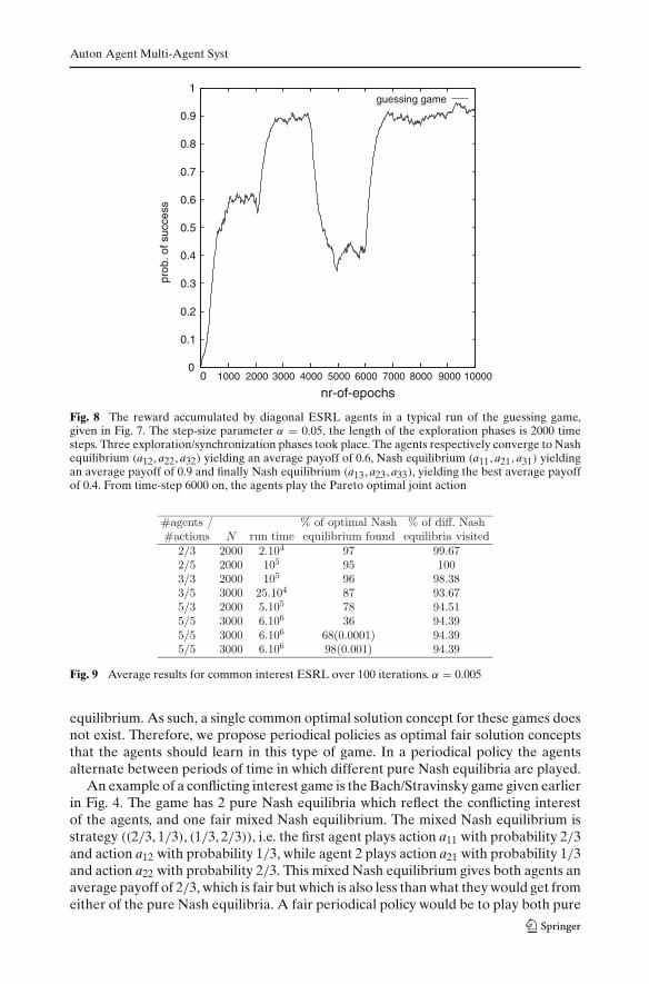
Figure 8 shows the working of ESRL for the diagonal game of Fig. 7. The plot onlygives information on one run of the algorithm. Agents can possibly find different Nashequilibria during the different phases, therefore average results do not make sensehere. In the guessing game the 3 pure Nash equilibria are located on the diagonal.These are all found during the three exploration phases of ESRL (Fig. 8). The lengthof each exploration or learning phase is fixed here on 2000 time steps. From time-step6000 on, the optimal joint Nash equilibrium is played, the agents’ private action spacesare reduced to a singleton.

In Fig. 9 average results are given for ESRL agents with random restarts learningin joint action spaces of different sizes. Random common interest games, for whichthe expected payoffs for the different joint actions are uncorrelated random numbersbetween 0 and 1 are generated. ESRL assures that an important proportion of theNash equilibria are visited. Almost 100% in small joint action spaces and still about94% in the larger ones. It may seem strange that although the optimal Nash equilibriais visited, the players sometimes do not recognize it. This is a consequence of thefact that rewards were stochastic and when payoffs are very close to each other, thesampling technique used here by the agents is not able to distinguish them. So actuallywhen convergence is not reached, agents still find extremely good solutions which arealmost as good as the optimal one. We tested this by relaxing convergence condi-tions in the last two experiments of Fig. 9. We considered the agents to be convergedwhen the difference in payoff of the joint action they recognized as the best and thetrue optimal one was no more than 0.0001 and 0.001, respectively. This increases thesuccess rate considerably as can be seen in Fig. 9.

5 ESRL in conflicting interest games

In this section, we introduce ESRL for stochastic conflicting interest games. For now,we assume that conflicting interest means that each agent prefers another pure Nash


0

0.1

0.2

0.3

0.4

0.5

0.6

0.7

0.8

0.9

1

0 1000 2000 3000 4000 5000 6000 7000 8000 9000 10000

prob

. of s

ucce

ss

nr-of-epochs

guessing game

Fig. 8 The reward accumulated by diagonal ESRL agents in a typical run of the guessing game,given in Fig. 7. The step-size parameter α = 0.05, the length of the exploration phases is 2000 timesteps. Three exploration/synchronization phases took place. The agents respectively converge to Nashequilibrium (a12, a22, a32) yielding an average payoff of 0.6, Nash equilibrium (a11, a21, a31) yieldingan average payoff of 0.9 and finally Nash equilibrium (a13, a23, a33), yielding the best average payoffof 0.4. From time-step 6000 on, the agents play the Pareto optimal joint action

Fig. 9 Average results for common interest ESRL over 100 iterations. α = 0.005

equilibrium. As such, a single common optimal solution concept for these games doesnot exist. Therefore, we propose periodical policies as optimal fair solution conceptsthat the agents should learn in this type of game. In a periodical policy the agentsalternate between periods of time in which different pure Nash equilibria are played.

An example of a conflicting interest game is the Bach/Stravinsky game given earlierin Fig. 4. The game has 2 pure Nash equilibria which reflect the conflicting interestof the agents, and one fair mixed Nash equilibrium. The mixed Nash equilibrium isstrategy ((2/3, 1/3), (1/3, 2/3)), i.e. the first agent plays action a11 with probability 2/3and action a12 with probability 1/3, while agent 2 plays action a21 with probability 1/3and action a22 with probability 2/3. This mixed Nash equilibrium gives both agents anaverage payoff of 2/3, which is fair but which is also less than what they would get fromeither of the pure Nash equilibria. A fair periodical policy would be to play both pure


Nash equilibria in turns, i.e. joint action (a11, a21) and (a12, a22). As a consequence,the average payoff for both agents will be 1.5.

The main idea of exploring selfish reinforcement learning agents is that agentsexclude actions from their private action space so as to further explore a reduced jointaction space. This idea is here used to let a group of agents learn a periodical policy.However, the agents may not have the same incentives to do this as in common inter-est games. As a result, we have to assume that agents will behave socially. Our ideasbehind the social behavior of agents were motivated by the Homo Egualis societyfrom sociology [6]. In a Homo Egualis society, agents do not only care about theirown payoff, but also about how it compares to the payoff of others. A Homo Egualisagent is displeased when it receives a lower payoff than the other group members, butit is also willing to share some of its own payoff with the others when it is winning.Very limited communication between the agents will be needed to implement theHomo Egualis idea, i.e. the comparison of payoff to decide which agent is best off.For the rest, agents remain independent.

5.1 Learning a periodical policy with ESRL

The exploration phase and synchronization phase for ESRL in conflicting interestgames is given in Algorithms 4 and 5. The exploration phase is more or less the samethan the one given in Algorithm 1. However, here we present a version with real-valued rewards instead of binary rewards. The Q-learning update rule for statelessenvironments is used to calculate the average reward of private actions. For each ac-tion ai in agent j’s action space, a Q-value vi is associated. These values are normalizedinto action probabilities pi for the action selection process. Agent j now calculates aglobal average reward average for the whole learning process.

Algorithm 4 Exploration phase for ESRL agent j in conflicting interest gamesInitializetime step t⇐ 0 ,for all actions i that are not excluded :initialize action values vi(t) and action probabilities pi(t)(assume l = |Aj| and k ≤ l is the number of not excluded actions)repeat

t := t + 1choose action ai in Aj probabilistically using p(t − 1) = (p1(t − 1), . . . , pl(t − 1))

take action ai, observe immediate reward r in [0, 1]with a given learning rate α, update the action value as follows:

vi(t) ⇐ (1− α)vi(t − 1)+ αr

for action ai

vi′ (t) ⇐ vi′ (t − 1)− αvi′ (t − 1)


normalize the action values vi(t) in probabilities pi(t)set the global average: average⇐ t−1

t average+ rt

until t = N

In ESRL the best performing agent gives the other agents the chance to increasetheir payoff. All agents broadcast their global average average as well as the average


payoff vi(N) that was collected for the private action ai to which the agent convergedduring the previous exploration phase. The agent who experienced the highest cumu-lative payoff and the highest average payoff during the last exploration phase, willexclude the action it is currently playing so as to give the other agents the opportunityto converge to a more rewarding situation. So after finding one of the Nash equilibria,all the joint actions containing the action of the best performing agent are temporarilyremoved from the joint action space. A new exploration phase is started in which theresulting action subspace is explored. During this second exploration phase the groupwill reach another Nash equilibrium and one of the other agents might have caughtup with the former best agent. At this point, communication takes place and the cur-rently “best" agent can be identified. Note that not only the reward accumulated inthe previous exploration phase is used to select the best performing player, also thecumulative payoff or global average is needed to see if an agent needs more time tocatch up with the others. Only the agent that is recognized as the best in the abovesense, has action(s) excluded in its private action space. If some other agent becomesthe best, the previous best agent can use its full original action space again.

In this ESRL version, the phases given by Algorithms 4 and 5 should alternateuntil the end of the learning process. As a result agents play a periodical policy, theyalternate between the different Nash equilibria of the game.

Algorithm 5 Synchronization phase for ESRL agent j in conflicting interest gamesT ← T + 1get action ai in Aj for which the action probability pi((T − 1)N) ≈ 1

broadcast action value vj = vi((T − 1)N) and global averagej = average to all other agentsreceive action value vb and global average averageb for all agents bif vj > vb and averagej > averageb for all b then

temporarily exclude action ai : Aj ⇐ Aj\{ai}else

restore the original action set: Aj ⇐ {a1, . . . , al} with l = |Aj|end if

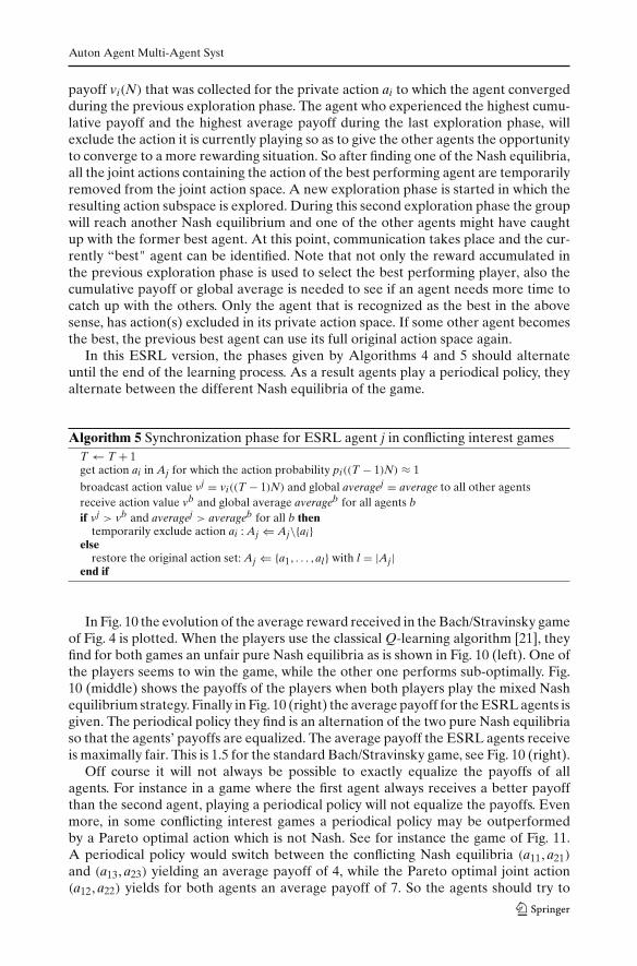
In Fig. 10 the evolution of the average reward received in the Bach/Stravinsky gameof Fig. 4 is plotted. When the players use the classical Q-learning algorithm [21], theyfind for both games an unfair pure Nash equilibria as is shown in Fig. 10 (left). One ofthe players seems to win the game, while the other one performs sub-optimally. Fig.10 (middle) shows the payoffs of the players when both players play the mixed Nashequilibrium strategy. Finally in Fig. 10 (right) the average payoff for the ESRL agents isgiven. The periodical policy they find is an alternation of the two pure Nash equilibriaso that the agents’ payoffs are equalized. The average payoff the ESRL agents receiveis maximally fair. This is 1.5 for the standard Bach/Stravinsky game, see Fig. 10 (right).

Off course it will not always be possible to exactly equalize the payoffs of allagents. For instance in a game where the first agent always receives a better payoffthan the second agent, playing a periodical policy will not equalize the payoffs. Evenmore, in some conflicting interest games a periodical policy may be outperformedby a Pareto optimal action which is not Nash. See for instance the game of Fig. 11.A periodical policy would switch between the conflicting Nash equilibria (a11, a21)

and (a13, a23) yielding an average payoff of 4, while the Pareto optimal joint action(a12, a22) yields for both agents an average payoff of 7. So the agents should try to


0.4

0.6

0.8

1

1.2

1.4

1.6

1.8

2

0 1000 2000 3000 4000 5000 6000 7000 8000 9000 10000

pay-

off

pay-

off

pay-

off

time0 1000 2000 3000 4000 5000 6000 7000 8000 9000 10000

time

player 1player 2

player 1player 2

player 1player 2

0.6

0.7

0.8

0.9

1

1.1

1.2

1.3

1.4

1.5

1.6

0.6

0.7

0.8

0.9

1

1.1

1.2

1.3

1.4

1.5

1.6

0 500 1000 1500 2000 2500 3000 3500 4000 4500 5000

time

Fig. 10 Learning in the Bach/Stravinsky game of Fig. 4. Left: the average payoff for 2 Q-learnersconverging to one of the Nash equilibria, Middle: the average payoff for 2 agents playing the mixedNash equilibrium, Right: the average payoff for 2 Homo Egualis ESRL agents playing a periodicalpolicy

a21 a22 a23

a11 (7,1) (0, 0) (0, 0)a12 (0,0) (7, 7) (0,10)a13 (0,0) (10,0) (1, 7)

Fig. 11 A 2 player with 2 conflicting Nash equilibria, (a11, a21) and (a13, a23) and a Pareto optimaljoint action (a12, a22), which is not Nash

learn, when periodical policies are interesting, i.e. optimal and fair. In the next sectionESRL agents are faced with games of which they do not know the type in advance. Thegoal of learning is to find an optimal fair solution, which may or may not be periodical.

6 Learning in non-zero sum games

In this section we generalize ESRL to general non-zero sum games, of which the agentsdo not know the type in advance, i.e. pure common interest or conflicting interest. Inthis case, the objective of the ESRL agents is to learn a good fair solution, which can


be a periodical policy when conflicting interests are present and which should be thePareto Optimal solution when the agents’ interests coincide.

6.1 The general synchronization phase

When the agents use the ESRL algorithm for learning in common-interest games, i.e.Algorithm 1 combined with Algorithm 3 they will know at the end of explorationwhether the game they are playing is pure common interest or not. Indeed, whenexploitation begins the agent will notice after a while if its performance achieves thesame level that was reached during learning. If it does, the game must be commoninterest and the agents coordinate on the same joint action that the agents recognizedas the best during learning. If not, clearly the agents did not coordinate on the samesolution and thus either conflicting interests exists or the Pareto optimal solution isnot found yet. Anyhow, in the latter situation exploration should start over again,because for now the agents only have individual information on the joint actions theyvisited, which is not enough to find an optimal fair (periodical) policy for all agents.So, preferably after every exploration phase the agents should broadcast their per-formance as in the synchronization phase of Algorithm 5, so that at the end of allexploration/synchronization phases, a fair possible (periodical) policy can be formed.The idea is to combine both previous versions of the synchronization phase. Then wecan use random restarts to move more quickly through the joint action space, togetherwith broadcasts to share the preference the agents have on the joint actions convergedto. The generalized synchronization phase is given in Algorithm 6.

Each agent keeps the payoff information from the previous exploration phase in ahistory list, called hist. An element of hist consists of the private action the agent con-verged to and a payoff vector, containing the payoff received by all the agents duringthe previous phase. So, each agent stores its own private action combined with a payoffvector

→v . This vector is the same for all agents. Important is that the list hist keeps the

original order of its elements. At the end of all phases, the Pareto optimal elementsof list hist are filtered. Since this operation only depends on the payoff vectors, eachagent filters the same elements from its list hist. With these remaining elements theagent can now build a policy. Beforehand, the system designer can specify what thispolicy should look like. He can set the policy of each agent to action amin, for which theassociated payoff vector

→v is most fair in the sense that the variation in payoff between

the players, denoted by s is minimal for→v . Since the agents have the same payoff vec-

tors in the same order in their list, they can independently set this policy that allowsthem to select the best, fair joint action they encountered together during learning.A periodical policy can also be built; for instance include in each agent’s policy thoseactions, whose associated payoff vectors have a deviation which is close to the devi-ation of the most fair payoff vector in the history list. This closeness can be set usingparameter δ. Other policies with all elements of the history list can also be defined.As such, different agents’ objectives can be specified at the beginning of learning.

A practical improvement that was added, is that the length of the explorationphase is no longer preset. Instead, the agents decide for themselves when their actionprobabilities have converged sufficiently and when this is the case, they broadcasttheir payoff. In practice this happens when an action exists, for which the probabilityof being selected is more than a predefined number 0 � ζ < 1. The synchroniza-tion phase starts when the agent received the broadcast information from all otheragents. However, not implemented here, statistical tests could be added to help the


Algorithm 6 Synchronization phase for ESRL agent j in non-zero sum games. Theagents’ objective is to find the optimal fair solution

if T ≤M (M = total number of exploration phases to be played) thenT ⇐ T + 1get action ai in Aj for which pi((T − 1)N) ≈ 1

broadcast action value vj = vi((T − 1)N) to all other agentsreceive action value vb of all agents bupdate history hist with action (ai) and payoff vector

→v = (v1, . . . , vn), i.e.:

hist(T)⇐ hist(T − 1) ∪ (ai,→v )

if |Aj| > 1 thentemporarily exclude action ai : Aj ⇐ Aj\{ai}

elserestore the original action set: Aj ⇐ {a1, . . . , al} with l = |Aj|

end ifelse if T =M then

collect Pareto optimal actions from history: PO(hist)compute for every

→v ∈ PO(hist), deviation s i.e.

s(→v ) =

∑nj (vj −

∑nj vj

n )2

n− 1

set policy : take δ ≥ 0 , set amin :

amin ⇐ {ai|(ai,→v ) ∈ PO(hist) and s(

→v ) is minimal}

if δ = 0 then

policy⇐ amin

elsemake policy periodical:

policy⇐ {ai|(ai,→v ) ∈ PO(hist) and s(

→v ) ≤ s(

→v min)+ δ}

end ifend if

agents to decide when convergence has happened and when the average reward isapproximated accurately. An example test is given in [3].

The general ESRL algorithm is demonstrated on the testbed games of Fig. 12.Important to notice is that the agents do not know the type of game beforehand. Theresults for a typical run of the games can be found in Fig. 13 (left) and (right), respec-tively. For both games the Pareto optimal equilibrium is found. The agents find allequilibria and at the end the set of Pareto optimal solutions drawn from their history isa singleton. The time steps needed before the optimum is reached, is comparable withthe earlier versions of ESRL. Off course, just as before, when different equilibria existwith payoffs very close to each other, it can be difficult for the agents to recognize thegenuine best one. In this case the agents may form a periodical policy or identify theother joint action as the best. However when this happens, all agents will decide to doso and the overall payoff information gathered will still be very close to the optimal.


Fig. 12 Stochastic versions of the climbing game and penalty game (k = −50). With each joint actionan expected reward is associated that represents the probability of success for that action

0

0.1

0.2

0.3

0.4

0.5

0.6

0.7

0.8

0.9

1

0 5000 10000 15000 20000 25000 30000

pay-

off

pay-

off

time

player 1player 2

player 1player 2

0

0.1

0.2

0.3

0.4

0.5

0.6

0.7

0.8

0.9

1

0 5000 10000 15000 20000 25000 30000

time

Fig. 13 Generalized ESRL learning in common interest games. Left: Average payoff in the climbinggame of Fig. 12. Right: Average payoff in the penalty game of Fig. 12. Step size parameter α = 0.05,while δ = 0. The agents decide for themselves when an exploration phase can be ended

The behavior of generalized ESRL in conflicting interest games is illustrated bythe results of Fig. 14. On the left side the average payoff for a typical run of the sto-chastic variant of the Bach/Stravinsky game is given, the right side gives the averagepayoff for a typical run of the stochastic version of the Prisoner’s dilemma game. Thestochastic version of both games we used, is given in Fig. 15. Again, the generalizedESRL behaves optimally. In the first game, a periodical policy consisting of the twopure Nash equilibria is found. In the second game, the best Pareto optimal Nashequilibrium is found.

How well the agents approximate the expected rewards of the joint actions influ-ences the behavior of the algorithm. For instance, in the Bach/Stravinsky game, thedeviation s of the 2 pure Nash equilibria could be seen as being different by the agentsbecause of the stochasticity. As such the agents may decide to choose one of theminstead of agreeing on a periodical policy. In this case it is a good idea to relax theassumption that only the action with the minimal deviation in the players’ payoff ischosen. Instead all the actions for which the deviation of the associated payoff vectoris close to minimal could be added to the policy.

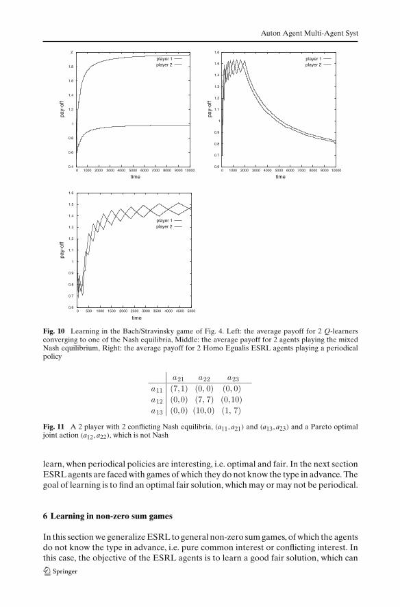
Figure 16 gives results for randomly generated non-zero sum games with a vary-ing number of agents n and actions l. The expected payoffs for the different jointactions are uncorrelated random numbers between 0 and 1. Results are averagedover 50 different games, each run 10 times. For these randomly generated games,as can be seen from Column 2 and 3 the number of Nash equilibria only slightlyincreases with enlarging joint action space, while the number of Pareto optimal jointactions increases rapidly. Columns 6 and 8 give average information on the optimal


0

0.1

0.2

0.3

0.4

0.5

0.6

0.7

0.8

0.9

1

0 5000 10000 15000 20000 25000 30000

pay-

off

pay-

off

time 0 5000 10000 15000 20000 25000 30000

time

0

0.1

0.2

0.3

0.4

0.5

0.6player 1player 2

player 1player 2

Fig. 14 Generalized ESRL learning in conflicting interest games. Left: Average payoff in a stochasticversion of the Bach/Stravinsky game. Right: Average payoff in a stochastic version of the prisoner’sdilemma. Step size parameter α = 0.05 and δ = 0. The agents end the exploration phase when theiraction probabilities have converged

Fig. 15 Stochastic versions of the Prisoner’s Dilemma Game (left) and the Bach/Stravinsky game(right). With each joint action an expected reward is associated, which represents the probability ofsuccess (reward 1) for that action

solution, i.e., the Pareto Optimal solution present in the game, with minimal deviations between the agents’ payoff. How well the agents play the game can be found inColumn 7 and 9. In all cases, the average best payoff found after learning (Column7) and the corresponding deviation between the agents for this solution (Column 9)is very close to the optimal results given in Columns 6 and 8, respectively. So, evenfor large joint action spaces, the agents are able to find interesting Pareto optimalsolutions, for which the payoff is fairly distributed between the agents in a mod-erate number of exploration/synchronization phases. For instance in the 5-player,5-actions games on average only 124.88 phases were played, while in the 7-player, 3-actions games only 175.9 phases were played on average. A typical run for a randomlygenerated 5-agent game, with each agents having 5 actions (and thus a joint actionsspace of 3125 joint actions) is given in Fig. 17. In the left experiment of Fig. 17, totallearning time, i.e. the time the agents use for playing exploration/synchronization isset to 80, 000 time steps, whereas for the experiment on the right of Fig. 17, learningtime is set to 200, 000 time steps. In the first experiment with limited exploration time,a reasonable fair solution was found. By letting the agents play more exploration/syn-chronization pairs, the average performance of all the agents increases. In fact in theexperiment on the right the agents play the optimal solution, as defined by the givenobjective.


Fig. 16 General ESRL agents in random generated non-zero sum games. αreward = 0.005, totallearning time is maximal = 400.000 time steps for the large joint action spaces, δ = 0 and the agentsdecide for themselves when their action probabilities have converged and thus when their explorationphase can be ended. The percentage of convergence to the optimal solution is 35% for the 5-player,5-action experiment and 50% for the 7-player, 3-action experiment

0

0.1

0.2

0.3

0.4

0.5

0.6

0.7

0.8

0.9

1

0 20000 40000 60000 80000 100000 120000 140000

pay-

off

pay-

off

time

player 1player 2player 3player 4player 5

player 1player 2player 3player 4player 5

0

0.1

0.2

0.3

0.4

0.5

0.6

0.7

0.8

0.9

1

0 50000 100000 150000 200000 250000 300000time

player 1

player 4

Fig. 17 Average payoff for generalized ESRL agents in a randomly generated game with 5 agents,each having 5 actions. Left: exploitation begins after 80,000 time steps. Right: exploitation begins after200,000 time steps. Step size parameter α = 0.05 and δ = 0. The agents decide for themselves whenan exploration phase can be ended

7 Adaptive load-balancing of parallel applications

In this section, the robustness of ESRL to delayed rewards and asynchronousaction selection is illustrated with the problem of adaptive load-balancing parallelapplications.

Load balancing is crucial for parallel applications since it ensures a good use of thecapacity of the parallel processing units. Here we look at applications that put highdemands on the parallel interconnect between nodes in terms of throughput. Exam-ples of such applications are compression applications which both process importantamounts of data and require a lot of computations. Data intensive applications usu-ally require a lot of communication and are therefore dreaded for most parallelarchitectures. The problem is exacerbated when working with heterogeneous parallelhardware.

A traditional architecture to use, is the master–slave software architecture, illus-trated in Fig. 18. In this architecture the slaves (one per processing unit) repeatedly re-quest a chunk of a certain size from the master. As soon as the data has been processed


SLAVE 1 SLAVE 2 SLAVE n

MASTER

...

communication bottleneck

1.request chunk

2.send chunk

3.data crunching

4.send results

Fig. 18 Master/Slave computation model

the result is transferred to the master and the slave sends a new request. This classicalapproach is called job farming. This scheme has the advantage of being both simple andefficient. Indeed, in the case of heterogeneous hardware the load (amount of processeddata) will depend on the processing speed of the different processing units. Faster pro-cessing units will more frequently request data and thus be able to process more data.

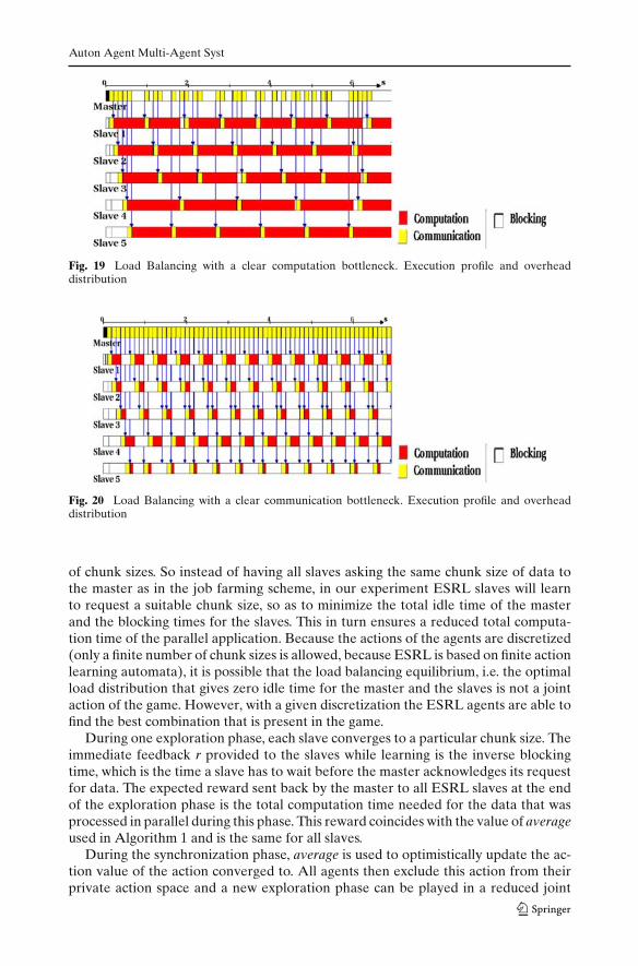
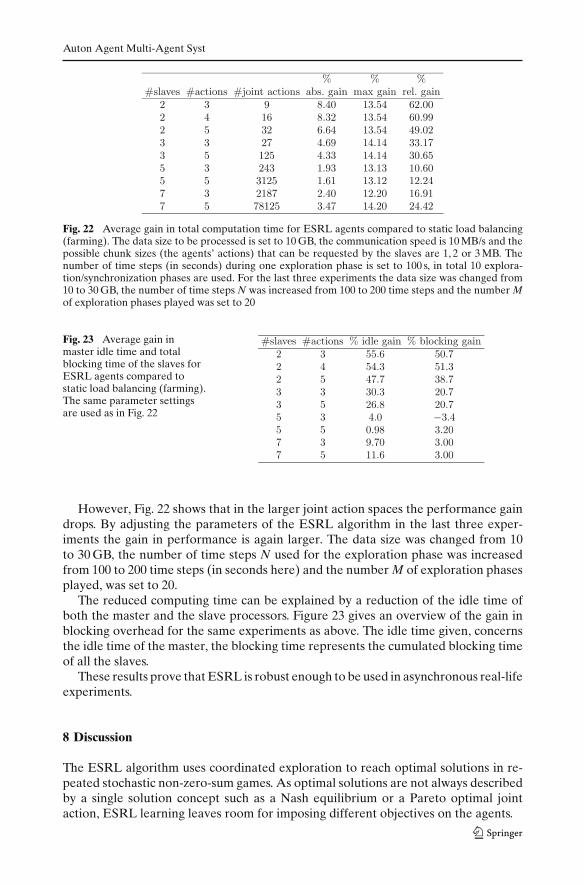
The bottleneck of data intensive applications with a master–slave architecture is thelink connecting the slaves to the master. In the presented experiments all the slavesshare a single link to their master. In an optimal load balancing setting, master andslave processors never become idle. This means that the processors are either commu-nicating or computing. The master is able to serve the slaves constantly and all pro-cessors work at 100% efficiency. One can say that in this situation, the communicationbandwidth of the master equals the computation power of the slaves. In all other cases,there will be either a clear communication or a computation bottleneck, what makesadaptive load balancing unnecessary. For instance, when the total computation powerof the slaves is lower than the master’s communication bandwidth, the master will beable to serve the slaves constantly and the slaves will work at full efficiency. However,the master has non-zero idle time and as such more slaves could be added to increasethe speedup. This situation is depicted in Fig. 19. When the total computation power ofthe slaves increases, the master will get request at a high rate and the communicationbecomes the bottleneck. The slaves will block each other because they are waiting to beserved and the total efficiency of the system drops. Figure 20 shows this latter situation.

In the following experiments we will only consider the settings in which computa-tional power and communication matches. We will assume that the slave processorsare heterogeneous and as such workload assignment and synchronization becomesnecessary. The equilibrium point represents an ideal load distribution, meaning thatthe master can serve the slaves constantly and keep them fully busy.

7.1 Learning to request data using ESRL

The problem defined above can be viewed as a single stage common interest coordi-nation problem. The actions of the agents consists of different chunk sizes the slavecan request from the master. A joint action of this game is therefore a combination


Fig. 19 Load Balancing with a clear computation bottleneck. Execution profile and overheaddistribution

Fig. 20 Load Balancing with a clear communication bottleneck. Execution profile and overheaddistribution

of chunk sizes. So instead of having all slaves asking the same chunk size of data tothe master as in the job farming scheme, in our experiment ESRL slaves will learnto request a suitable chunk size, so as to minimize the total idle time of the masterand the blocking times for the slaves. This in turn ensures a reduced total computa-tion time of the parallel application. Because the actions of the agents are discretized(only a finite number of chunk sizes is allowed, because ESRL is based on finite actionlearning automata), it is possible that the load balancing equilibrium, i.e. the optimalload distribution that gives zero idle time for the master and the slaves is not a jointaction of the game. However, with a given discretization the ESRL agents are able tofind the best combination that is present in the game.

During one exploration phase, each slave converges to a particular chunk size. Theimmediate feedback r provided to the slaves while learning is the inverse blockingtime, which is the time a slave has to wait before the master acknowledges its requestfor data. The expected reward sent back by the master to all ESRL slaves at the endof the exploration phase is the total computation time needed for the data that wasprocessed in parallel during this phase. This reward coincides with the value of averageused in Algorithm 1 and is the same for all slaves.

During the synchronization phase, average is used to optimistically update the ac-tion value of the action converged to. All agents then exclude this action from theirprivate action space and a new exploration phase can be played in a reduced joint


action space. At the end of all exploration/synchronization phases, the bestcombination found is exploited.

Note that the slaves use a real-numbered reward version of ESRL Algorithms 1and 3. Note also that since their is already communication between the master and theslaves, no extra communication overhead is created when the average reward is sendback at the end of each exploration phase. There is also no communication necessarybetween the slaves. As such ESRL can easily be implemented without introducingnew overheads in the parallel system.

This model has been simulated using the PVM [5] message-passing library toexperiment with the different dimensions of the problem. The application has beendesigned not to perform any real computation, but instead it replaces the computa-tion and communication phases by delays with equivalent duration. The global goal isminimizing the total computation time. A typical experiment consists of computation,communication and blocking phases. The data size to be processed is set to 10 GB, thecommunication speed is 10 MB/s and the possible chunk sizes (the agents’ actions)that can be requested by the slaves are 1, 2 or 3 MB. For the ESRL algorithm, thenumber of time steps during one exploration phase is set to 100 s, in total 10 explo-ration/synchronization phases are used. The hardware heterogeneity of the setup issimulated so that there is a match between the system’s communication bandwidthand total processing power. Figure 21 shows the time course of 3 ESRL slaves af-ter learning. One can observe that the slaves have learned to distribute the requestsnicely and hence use the link with the master efficiently. Slave 3 which is the fastestprocessor, with lowest granularity, is served constantly and has no idle time. Slave 2has some idle time, however it is the slowest processor.

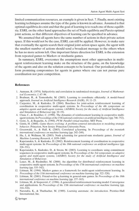
As shown in Fig. 22 we have run several experiments in different sized joint ac-tion spaces. The 4th column gives the absolute gain in total computation time for theESRL agents/slaves compared to the total computation time for the classical farmingapproach. The 5th column gives the gain in total computation time, which is maximalpossible for the given setting. The total computation time can only decrease when theidle time of the master is decreased. No gain is possible on the total communicationtime of the data. The last column gives the absolute gain compared to the gain thatwas maximally possible. In all experiments, considerable improvements were made.The ESRL agents are able to find settings in which the faster slave is blocked lessfrequently than the others.

Fig. 21 Execution profile of the exploitation phase of a typical experiment with 3 slaves


Fig. 22 Average gain in total computation time for ESRL agents compared to static load balancing(farming). The data size to be processed is set to 10 GB, the communication speed is 10 MB/s and thepossible chunk sizes (the agents’ actions) that can be requested by the slaves are 1, 2 or 3 MB. Thenumber of time steps (in seconds) during one exploration phase is set to 100 s, in total 10 explora-tion/synchronization phases are used. For the last three experiments the data size was changed from10 to 30 GB, the number of time steps N was increased from 100 to 200 time steps and the number Mof exploration phases played was set to 20

Fig. 23 Average gain inmaster idle time and totalblocking time of the slaves forESRL agents compared tostatic load balancing (farming).The same parameter settingsare used as in Fig. 22

However, Fig. 22 shows that in the larger joint action spaces the performance gaindrops. By adjusting the parameters of the ESRL algorithm in the last three exper-iments the gain in performance is again larger. The data size was changed from 10to 30 GB, the number of time steps N used for the exploration phase was increasedfrom 100 to 200 time steps (in seconds here) and the number M of exploration phasesplayed, was set to 20.

The reduced computing time can be explained by a reduction of the idle time ofboth the master and the slave processors. Figure 23 gives an overview of the gain inblocking overhead for the same experiments as above. The idle time given, concernsthe idle time of the master, the blocking time represents the cumulated blocking timeof all the slaves.

These results prove that ESRL is robust enough to be used in asynchronous real-lifeexperiments.

8 Discussion

The ESRL algorithm uses coordinated exploration to reach optimal solutions in re-peated stochastic non-zero-sum games. As optimal solutions are not always describedby a single solution concept such as a Nash equilibrium or a Pareto optimal jointaction, ESRL learning leaves room for imposing different objectives on the agents.


Different interesting efforts to augment standard RL techniques to the multi-agentcase can be found in MARL literature. They can be classified according to the typeof games they solve and the type of agents they use.

8.1 Related work

One of the first theoretical results of reinforcement learning in games, was achieved byLittman [12] . A Q-learning algorithm, called minimax-Q was developed for learningin zero-sum two-player games. The minimax of the Q-values were used in the updateof the value function. Afterward, convergence results were attained for minimax-Qin [14].

For common interest games, and in particular identical payoff games different ap-proaches exist. In [11] a convergence proof for independent optimistic Q-learnersin coordination games is given, however the algorithm is not suited for games withstochastic rewards. In [4] joint action learners are introduced. Joint action learnersexplicitly take the other agents into account, by keeping beliefs on their action selec-tion, based on procedures known as fictitious play in game theory. Assumed is thatthe actions of the others can be observed, though this is not sufficient to guaranteeconvergence to optimal equilibria.

In [3] simple joint action learning algorithms are proposed as baselines for anyfuture research on joint-action learning of coordination in cooperative MAS. Thealgorithms studied in [3] use fairly simple action selection strategies that are still guar-anteed to convergence to the optimal action choice. As the general ESRL algorithmof this paper also uses communication one could wonder why not use simple jointaction learners instead. The advantage of ESRL is that communication is only nec-essary when attractor points are reached at the end of an exploration phase. As suchcommunication only occurs for the interesting joint actions and not for all joint actionstaken, as is the case for joint action learners. This will make ESRL much more suitableto implement in a distributed setting. Moreover, the amount of communication willgrow exponentially with the number of agents and actions for joint action learners.

Several optimistic heuristic methods are proposed to guide action selection to opti-mal equilibria. In [9] the Q-value of an action in the Boltzmann exploration strategy, ischanged by an heuristic value, taking into account how frequently an action producesits maximum corresponding reward. This heuristic, which is called FMQ is suited forpure independent agents. It performs well in games with deterministic rewards. How-ever, in games with stochastic rewards the heuristic may perform poorly. Thereforethe authors propose the use of commitment sequences in [10] to allow for stochasticrewards. In a way these commitment sequences are very similar to the explorationphases of ESRL learning, however the former approach strongly depends on synchro-nous action-selection, whereas ESRL is suited for asynchronous real-life applicationsas shown in Sect. 7.

In [2] model-based algorithms are proposed for coordination in stochastic com-mon-interest games under imperfect monitoring. The learning algorithm is provedto have a polynomial-time convergence to a near-optimal value of the game. Themain difference with ESRL is that the games considered in [2] have determinis-tic rewards taken from the interval of real numbers [0, Rmax]. The transition func-tion between the stage games is stochastic, whereas in the work presented here, thereward function itself is stochastic, which makes ESRL robust to use in real-life exper-iments. The underlying idea of [2] is for the agents to find a common order over joint


actions, so that these can all be jointly executed. Since payoffs are identical for allagents, all agents build the same model and in fact what happens is a distributed coordi-nated execution of a single-agent reinforcement learning algorithm, which is R-MAXin the case of [2]. In contrast, the agents applying the ESRL algorithm do not have toexecute all joint actions together, they only need to find the interesting attractor pointsof the game, to which they will be driven by the learning automata. This makes ESRLmore scalable. Besides this, ESRL is also applicable for conflicting interest games.

As opposed to learning in non-zero sum games and common interest games, theproblem of learning in general-sum games is not well understood. Several algorithmsare proposed, however as most work focuses on learning Nash equilibria as a centralsolution concept, a general treatment does not exists. Hu and Welmann [8], extendedminimax-Q to general sum games. Their algorithm called Nash-Q developed forjoint action learners, uses a Nash equilibrium computation rule in the update of theQ-values. However, only a limited type of games satisfy the assumptions necessaryfor convergence to be guaranteed. The Friend-or-Foe Q-learning algorithm (FFQ)of [13] solves the same classes of games, however it doesn’t require Q-functions foropposing players to be optimized. Instead FFQ agents require to be told whetheran opposing agent is a friend or a foe. In the first case, FFQ results in the agentsmaximizing their own payoff and in the latter case the agents update their Q-values asin minimax-Q. Only when a coordination equilibrium or an adversarial equilibrium8

exist, convergence to a Nash equilibrium is guaranteed.We propose the use of periodical policies as optimal fair solutions in games of

conflicting interest like the Bach/Stravinsky game of Fig. 4. In [7], Correlated Q-learning (CE-Q) is proposed. Correlated Q-learning generalizes Nash-Q and FFQand is empirically demonstrated to converge to correlated equilibria. A correlatedequilibrium, a concept introduced by Aumann [1] is a generalization of a Nash equi-librium where each player may receive a private recommendation signal before thegames is played. These signals do not affect the payoff, but the players may base theirchoices on the signals received. A correlated equilibrium results if each player realizesthat the best he can do is to follow the recommendation, provided that all other play-ers will do this too. In the same way as a periodical policy, a correlated equilibrium canachieve higher rewards than a mixed Nash equilibrium by avoiding undesirable jointactions such as (Bach, Stravinsky) or (Stravinsky, Bach) in the Bach/Stravinsky gameof Fig. 4. However, to learn a correlated equilibrium in [7] Q-tables should be sharedamong the agents and thus all agents’ actions and rewards must be fully observable.In contrast, a periodical policy can be learned decentralized using ESRL which onlyrelies on a simple synchronization mechanism, whereas for correlated equilibria acentral planner is necessary.

8.2 Concluding remarks

Compared to the techniques reported in literature, ESRL agents are unique on differ-ent levels. For a start, ESRL is a technique for independent agents learning in a non-zero sum game with stochastic rewards. No beliefs are maintained about the actionsof others, which makes the algorithm simple and easy to use also in more than 2 playergames. Moreover no assumptions are made on the observability of the other agents’payoff or actions, which makes it possible to use ESRL in distributed systems with

8 An adversarial equilibrium is a Nash equilibrium with the extra property that no agent is hurt byany change in strategy by the other agents.


limited communication resources, an example is given in Sect. 7. Finally, most existinglearning techniques assume the type of the game is known in advance. Assumed is thatoptimal equilibria do exist and that the goal of learning is to reach one of those equilib-ria. ESRL on the other hand approaches the set of Nash equilibria and Pareto optimaljoint actions, so that different objectives of learning can be specified in advance.

We assumed that all agents have the same number of actions in their private actionspace. If this would not be the case, ESRL can still be applied. However, to make surethat eventually the agents search their original joint action space again, the agent withthe smallest number of actions should send a broadcast message to the others whenhe has no more actions left. One important future direction for ESRL is the extensionfrom repeated games to Markov or stochastic games.

In summary, ESRL overcomes the assumptions most other approaches in multi-agent reinforcement learning make on the structure of the game, on the knowledgeof the agents and also on the solution concepts to be learned. Our periodical policiesform promising compromises for agents in games where one can not pursue purecoordination nor pure competition.

References

1. Aumann, R. (1974). Subjectivity and correlation in randomized strategies. Journal of Mathemat-ical Economics, 1, 67–96.

2. Brafman, R., & Tennenholtz, M. (2003). Learning to coordinate efficiently: A model-basedapproach. Journal on Artificial Intelligence Research (JAIR), 19, 11–23.

3. Carpenter, M., & Kudenko, D. (2004). Baselines for joint-action reinforcement learning ofcoordination in cooperative multi-agent systems. In Proceedings of the 4th symposium onadaptive agents and multi-agent systems, (AISB04) Society for the study of Artificial Intelligenceand Simulation of Behaviour (pp. 10–19).

4. Claus, C., & Boutilier, C. (1998). The dynamics of reinforcement learning in cooperative multi-agent systems. In Proceedings of the 15th national conference on artificial intelligence (pp. 746–752).

5. Geist, A., & Beguelin, A. (1994). PVM: Parallel virtual machine. MIT Press.6. Gintis, H. (2000). Game theory evolving: A problem-centered introduction to modeling strategic

behavior. Princeton, New Jersey: Princeton University Press.7. Greenwald, A., & Hall, K. (2003). Correlated q-learning. In Proceedings of the twentieth

international conference on machine learning (pp. 242–249).8. Hu, J., & Wellman, M. (2003). Nash q-learning for general-sum stochastic games. Journal of

Machine Learning Research, 4, 1039–1069.9. Kapetanakis, S., & Kudenko, D. (2002). Reinforcement learning of coordination in cooperative

multi-agent systems. In Proceedings of the 18th national conference on artificial intelligence (pp.326–331).

10. Kapetanakis, S., Kudenko, D., & Strens, M. (2003). Learning to coordinate using commitmentsequences in cooperative multi-agent systems. In Proceedings of the 3rd symposium on adaptiveagents and multi-agent systems, (AISB03) Society for the study of Artificial Intelligence andSimulation of Behaviour.

11. Lauer, M., & Riedmiller, M. (2000). An algorithm for distributed reinforcement learning incooperative multi-agent systems. In Proceedings of the 17th international conference on machinelearning (pp. 535–542).

12. Littman, M. (1994). Markov games as a framework for multi-agent reinforcement learning. InProceedings of the 11th international conference on machine learning (pp. 322–328).

13. Littman, M. (2001). Friend-or-foe q-learning in general-sum games. In Proceedings of the 18thinternational conference on machine learning (pp. 157–163).

14. Littman, M., & Szepesvári, C. (1996). A generalized reinforcement-learning model: Convergenceand applications. In Proceedings of the 13th international conference on machine learning (pp.310–318).

15. Narendra, K., & Thathachar, M. (1989). Learning automata: An introduction. Prentice-HallInternational, Inc.


16. Nash, J. (1950). Equilibrium points in n-person games. Proceedings of the national academy ofsiences 36, 48–49.

17. Nowé, A., Parent, J., & Verbeeck, K. (2001). Social agents playing a periodical policy. InProceedings of the 12th European conference on machine learning pp. 382–393. Freiburg,Germany: Springer-Verlag LNAI2168.

18. Osborne, J., & Rubinstein, A. (1994). A course in game theory. Cambridge, MA: MIT Press.19. Samuelson, L. (1997). Evolutionary games and equilibrium selection. Cambridge, MA: MIT Press.20. Sastry, P., Phansalkar, V., & Thathachar, M. (1994). Decentralized learning of nash equilibria

in multi-person stochastic games with incomplete information. IEEE Transactions on Systems,Man, and Cybernetics, 24(5), 769–777.

21. Sutton, R., & Barto, A. (1998). Reinforcement learning: An introduction. Cambridge, MA: MITPress.

22. Thathachar, M., & Sastry, P. (2002). Varieties of learning automata: An overview. IEEETransactions on Systems, Man, and Cybernetics, Part B: Cybernetics, 32(6), 711–722.

23. Tsitsiklis, J. (1994). Asynchronous stochastic approximation and q-learning. Machine Learning,16, 185–202.

24. Tuyls, K. (2004). Multiagent reinforcement learning: A game theoretic approach. PhD Thesis,Computational Modeling Lab, Vrije Universiteit Brussel, Belgium.

25. Verbeeck, K. (2004). Coordinated exploration in multi-agent reinforcement learning. PhD Thesis,Computational Modeling Lab, Vrije Universiteit Brussel, Belgium.

26. Verbeeck, K., Nowé, A., & Parent, J. (2002). Homo egualis reinforcement learning agents forload balancing. In Proceedings of the 1st NASA workshop on radical agent concepts, pp. 81–91.Springer-Verlag LNAI 2564.

Date post:	02-Apr-2018
Category:	Documents
Upload:	doanthuy
View:	218 times
Download:	0 times

Exploring selﬁsh reinforcement learning in … Agent Multi-Agent Syst DOI...

Documents