Sushil Thapa

EXPLORING THE IMPACT OF URBAN GROWTH ON LAND

SURFACE TEMPERATURE OF KATHMANDU VALLEY, NEPAL

EXPLORING THE IMPACT OF URBAN GROWTH ON LAND

SURFACE TEMPERATURE OF KATHMANDU VALLEY,

NEPAL

Dissertation Supervised by

Filiberto Pla Bañón, PhD

Professor, Dept. Lenguajes y Sistemas Informaticos

Universitat Jaume I, Castellón, Spain

Dissertation Co-supervised by

Pedro Cabral, PhD

Professor, Instituto Superior de Estatística e Gestão de Informação

Universidade Nova de Lisboa, Lisbon, Portugal

Edzer Pebesma, PhD

Professor, Institute for Geoinformatics

Westfälische Wilhelms-Universität, Münster, Germany

February 2017

I

ACKNOWLEDGEMENTS

I am very much delighted to express my profound gratitude to all the generous

people for their help and support. My Masters endeavor has been an amazing

learning experience and this dissertation would not have been accomplished without

them.

First of all, I am very much grateful to my supervisor and co-supervisors: Prof. Dr.

Filiberto Pla Banon, Prof. Dr. Pedro Cabral and Prof. Dr. Edzer Pebesma for their

valuable suggestions and remarks.

I would like to extend my sincere gratitude to Dr. Pedro Latorre Carmona,

Department of Computer Languages and Systems, UJI for his encouragement,

guidance and constructive criticisms throughout the project.

I would also greatly acknowledge professors Joaquin Huerta, Christoph Brox, Marco

Painho, Michael Gould, Christian Kray for the excellent organization of the Master’s

Program.

I am highly obliged in taking the opportunity to sincerely thank all my professors

from UJI and ifgi who bestowed me with multidisciplinary knowledge and skills and

helped to develop professionalism in me.

I am duly grateful to European Commission for granting me with the scholarship to

pursue my study here in Europe.

Special thanks to all the administrative staffs from UJI and ifgi who were always

kind to me. Thanks to all of my friends for sharing awesome memories.

I also express my sincere gratitude to my parents and brothers for their inspirations,

unconditional love and support.

II

EXPLORING THE IMPACT OF URBAN GROWTH ON LAND

SURFACE TEMPERATURE OF KATHMANDU VALLEY,

NEPAL

ABSTRACT

Kathmandu is experiencing rapid urban growth since last few decades. Cities are

expanding across the countryside at the expense of productive land. Such urban

sprawl has incurred adverse environmental consequences affecting quality of life of

urban residents in the valley. Recently, Kathmandu has been identified to be on the

verge of climate change, especially in the context of urban warming. Thus exploring

the impact of urban growth on land surface temperature could be an effective means

to unveil environmental issues caused by anthropogenic activities. This can be useful

for the urban planners in urban planning and management as well as to raise public

awareness regarding urban warming effect. Advancement in thermal Remote

Sensing, GIS and statistical procedure has enabled monitoring land surface

temperature and its correlation to land use and land cover. To analyze such

relationship, we performed supervised classification and change detection to

determine the spatial trend of land use and land cover change. After that we obtained

the spatial pattern of LST using thermal band of Landsat images. Then we applied

regression analysis to explore the relationship between surface temperature and land

surface characteristics including both land use land cover types and land use and land

cover indices. Based upon our analysis, we found that urban area has increased

considerably by 259% during the period 1988-2014. The surface temperatures were

found to be greater for bare soil and urban land use types. The regression analysis

showed positive correlation between urban growth and LST. Finally we found LULC

indices based approach better than LULC class for LST prediction.

III

KEYWORDS

Land use land cover

Land Surface Temperature

Landsat

Regression analysis

Thermal Remote Sensing

Urban fragmentation

Urban Growth

Urban Heat Island

IV

ACRONYMS

ADB Asian Development Bank

CBS Central Bureau of Statistics

CLEAR Center for Land Use Education and Research

DEM Digital Elevation Model

DHM Department of Hydrology and Meteorology

DoR Department of Roads

GCPs Ground Control Points

GIS Geographic Information System

ICIMOD International Center for Integrated Mountain Development

KRR Kernel Ridge Regression

LST Land Surface Temperature

LULC Land use land cover

NDBI Normalized Difference Built up Index

NDVI Normalized Difference Vegetation Index

NDWI Normalized Difference Water Index

RMSE Root Mean Square Error

UHI Urban Heat Island

UNOHCHR United Nations Office of the High Commissioner for Human Rights

WGS 84 World Geodetic System 84

V

TABLE OF CONTENTS

Contents

ACKNOWLEDGEMENTS .......................................................................................... I

ABSTRACT................................................................................................................. II

KEYWORDS ............................................................................................................. III

ACRONYMS ............................................................................................................. IV

1. INTRODUCTION ................................................................................................... 1

1.1 Background & Motivation ................................................................................. 1

1.2 Aim & Objectives .............................................................................................. 6

1.3 Research Questions ............................................................................................ 7

1.4 Research Structure ............................................................................................. 7

2. DATA & STUDY AREA ........................................................................................ 9

2.1 Data .................................................................................................................... 9

2.2 Software ........................................................................................................... 10

2.3 Data Preparation ............................................................................................... 10

2.4 Study area ......................................................................................................... 11

3. RESEARCH METHODS ...................................................................................... 14

3.1 Supervised Maximum Likelihood Classification ............................................. 14

3.2 Accuracy Assessment ...................................................................................... 15

3.3 Land Surface Temperature Retrieval ............................................................... 16

3.4 Land use Land Cover Indices ........................................................................... 19

3.5 Regression Analysis ......................................................................................... 20

3.5.1 Linear Regression ...................................................................................... 20

3.5.2 Non-linear Regression ............................................................................... 21

3.5.3 Experimental setup for the appropriate approach assessment for LST

prediction ................................................................................................... 22

3.6 Hot Spot Analysis ............................................................................................ 22

3.7 Urban Fragmentation ....................................................................................... 24

4. RESULTS & DISCUSSION ................................................................................. 26

4.1 Land use land cover change in the study area .................................................. 26

VI

4.2 Spatial pattern of LST and LULC indices........................................................ 36

4.2.1 Land Surface Temperature ........................................................................ 36

4.2.2 Normalized Difference Vegetation Index ................................................. 38

4.2.3 Normalized Difference Built-up Index ...................................................... 40

4.2.4 Normalized Difference Water Index ......................................................... 42

4.3 Relationship between LST & LULC characteristics ........................................ 44

4.3.1 Linear Regression of LST and LULC indices ........................................... 44

4.3.2 Linear Regression of LST and LULC class .............................................. 48

4.3.3 Assessment of LULC indices and LULC class based approach for LST

prediction ................................................................................................... 49

4.4 Impact of urban growth on UHI effect ............................................................. 51

5. CONCLUSION ...................................................................................................... 57

REFERENCES .......................................................................................................... 59

APPENDICES ........................................................................................................... 65

VII

LIST OF TABLES

Table 1: Detail Characteristics of images .................................................................... 9

Table 2: Parameters in LST Retrieval........................................................................ 19

Table 3: Accuracy Assessment of classified images for different years ................... 26

Table 4: Area statistics of land use land cover classes for 1988 to 2014 .................. 30

Table 5: Land use land cover change during 1988 - 2014 ......................................... 31

Table 6: Proportion of various urban growth types in different periods (%) ............ 35

Table 7: Proportion of various urban landscape types in different years (%) ........... 36

Table 8: Correlations between LST and LULC indices and DEM ............................ 45

Table 9: Regression Analysis Parameters .................................................................. 46

Table 10: Regression equations for each LULC class ............................................... 48

Table 11: RMSE values for LULC indices and linear regression case ..................... 49

Table 12: RMSE values for LULC indices and KRR case ........................................ 50

Table 13: RMSE values for LULC class and KRR case ........................................... 50

Table 14: Proportion of various thermal region in different LULC in 1988 (%) ...... 53

Table 15: Proportion of various thermal region in different LULC in 2000 (%) ...... 53

Table 16: Proportion of various thermal region in different LULC in 2014 (%) ...... 54

Table 17: Mean LST by urban landscape in degree Celsius...................................... 55

Table 18: Mean LST by urban growth type in degree Celsius .................................. 56

VIII

LIST OF FIGURES

Figure 1: Structure of the thesis ................................................................................... 8

Figure 2: 3D perspective of the study area ................................................................ 12

Figure 3: Location map of the study area .................................................................. 13

Figure 4: Land use land cover map of study area in 1988 ......................................... 27

Figure 5: Land use land cover map of study area in 2000…………………………..28

Figure 6: Land use land cover map of study area in 2014…………………………..29

Figure 7: Land use land cover areas in different years .............................................. 31

Figure 8: Percentage change in LULC between 1988 and 2000 ............................... 32

Figure 9: Percentage change in LULC between 2000 and 2014 ............................... 32

Figure 10: Percentage change in LULC between 1988 and 2014 ............................. 33

Figure 11: Urban growth types in different periods .................................................. 34

Figure 12: Urban landscape classes for different years ............................................. 35

Figure 13: LST of the study area for the years 1988, 2000 and 2014 ....................... 37

Figure 14: Mean LST for each LULC class .............................................................. 38

Figure 15: NDVI within each LULC class in 1988, 2000 and 2014 ......................... 39

Figure 16: Mean NDVI values for each LULC class in 1988, 2000 and 2014 ......... 40

Figure 17: NDBI within each LULC class in 1988, 2000 and 2014 ......................... 41

Figure 18: Mean NDBI values for each LULC class in 1988, 2000 and 2014 .......... 42

Figure 19: NDWI within each LULC class in 1988, 2000 and 2014 ........................ 43

Figure 20: Mean NDWI values for each LULC class in 1988, 2000 and 2014......... 44

Figure 21: Measured LST vs. Estimated LST for developed regression models ...... 47

Figure 22: Measured LST vs. Estimated LST for LULC indices and KRR case for

2000 ......................................................................................................... 51

Figure 23: Hot Spot Analysis of LST for different years .......................................... 52

Figure 24: LULC distribution (% area) in Hot Spot area .......................................... 54

Figure 25: Linear regression between urban cover and LST .................................... 56

1

1. INTRODUCTION

1.1 Background & Motivation

Urbanization is nowadays a rising trend globally, especially in an alarming rate in

developing countries. This makes cities around the world grow both in number and

size. Urban growth is indeed a development process that occurs over some period of

time, as city and its suburbs expand into an adjoining countryside. It is primarily

accredited to the population growth, as there is a global trend of thousands of people

migrating to the cities every year (Bekele, 2005).

Urban growth is characterized by the transformation of natural land covers into built

up areas (Rimal, 2011). It causes depletion of greenery in the cities and subsequent

increase in the impervious surface. Cities experience unprecedented changes in land

use and land cover patterns due to urban growth. As urban growth persists, studies

addressing their reciprocal impacts are gaining importance (Parker, 2010). Urban

growth has adverse impact on land surface characteristics including its thermal

capacity. The increased thermal storage capacity creates so called urban heat island

(UHI) effect, observed as an elevated temperature of urban areas relative to rural

ones, and it is an important research topic related to urban climate and environmental

studies (Stewart & Oke, 2012). UHI emerges through the modification of land

surface in a way that favors heat storage and trapping (e.g. reduced vegetation), and

anthropogenic heat release from vehicles, industries, and buildings (Oke, 1982;

Sailor & Lu, 2004). It is one of the perilous environmental issues, which can cause

negative impact on human and environment (Grimmond, 2007). It degrades air,

influences local climate, increases ground level ozone production (Lo et al., 2003),

and ultimately affects our quality of life. Therefore, the subject of urban growth and

UHI has drawn attention from ecologists, urban planners, sociologists,

administrators, policy makers, and finally to the urban residents (Bekele, 2005; Li et

al., 2012).

2

Numerous studies related to UHI have been carried out so far (Chen et al., 2006;

Coseo et al., 2015; Goward, 1981; Imhoff et al., 2010; Lo et al., 2003; Mirzaei, 2015;

Rizwan et al., 2008; Saito et al., 1996; Sun et al., 2012; SRIVANIT et al., 2012; Tan

et al., 2010; Tran et al., 2006; Weng et al., 2004; Yuan & Bauer, 2007). These

studies cover a wide range of topics related to UHI such as: the influence of urban

landscapes and LULC change in UHI phenomenon, spatial-temporal variation of

UHI, relationship between UHI and LULC indices, UHI modeling and simulation,

impact of UHI effect on heat wave and human welfare, and possible measures to

mitigate UHI effect. These studies provide a remarkable contribution to researchers

and policy makers concerned with UHI phenomenon.

Land Surface Temperature (LST) is an important parameter in the UHI phenomenon,

which manifests high spatial and temporal inhomogeneity especially in urban areas

(Zaksek & Ostir, 2011). LST is actually the skin temperature of the land surface

which differs from the land surface air temperature (SRIVANIT et al., 2012). It can

be derived from freely available data sources such as Landsat, MODIS and ASTER.

The thermal band of these sensors enables data collection on thermal properties of

the land surface based on the amount of emitted energy. Besides, such data can also

be used to monitor LULC change over time. Thus these two prospects enabled

researchers to explore the link between LULC change and LST change over time. In

this way, monitoring UHI effect due to LULC change has become feasible (Fabrizi et

al., 2010).

To obtain LST from thermal images, many algorithms have been proposed such as:

Single Channel, Split window, Mono window, Radiative transfer equation etc. (Qin

et al., 2001; Yu et al., 2014). However Split window relies on two spectrally adjacent

thermal bands, but Landsat 4, 5 and even ETM+ possess only one thermal band.

Thus this method is unsuitable for those images. Similarly the problem with the

Radiative transfer equation method is that it requires in-situ radio sounding to be

launched concurrently with satellite pass. Like Radiative transfer equation method,

Mono window method also involves various parameters such as effective mean

atmospheric temperature, emissivity and transmittance to be determined, which

3

requires in-situ measurement. Single Channel method on the other hand requires high

quality atmospheric transmittance code to estimate the atmospheric features involved

in the model, and is complicated. Therefore, explicitly an image based approach

utilizing surface emissivity representing the brightness temperature only, without

requiring atmospheric profile parameters has been considered in this study.

Surface emissivity is indispensable for LST inversion, specifically for the image

based method. Basically there are three methods to determine the land surface

emissivity: Classification based emissivity method, NDVI based method and

Temperature independent spectral indices method (Yu et al., 2014). For

Classification based emissivity method, surface emissivity is obtained from

classification image, but the emissivity value should be known in advance. This

requires good knowledge of the study area and emissivity measurement on surface

representative of different classes must be coincident with satellite transit time.

Temperature independent spectral indices method is also complicated. Hence due to

simplicity NDVI based method is suitable for our purpose.

Since LST has a direct link to the land surface characteristics (Quattrochi &Luvall,

1999) and on the other hand, LULC change is strongly related to the urban growth,

the study of the relationship between LST and LULC is fundamental to explore the

impact of urban growth on land surface temperature, including the UHI effect. The

study of the relationship between LST and LULC change helps researchers to

understand the cause, spatial-temporal distribution, consequences and possible

measures to mitigate the UHI effect.

LULC indices and LULC types are two major indicators of LULC mostly used in the

study of LST and LULC relationship. There are various types of LULC indices

proposed to investigate the correlations between LULC and LST. Amongst several

indices, Normalized Difference Vegetation Index (NDVI), Normalized Difference

Built up Index (NDBI) and Normalized Difference Water Index (NDWI) strongly

correlate with LST (Chen et al., 2006). These indices are extracted using band ratios

of different bands of satellite images. Each of these indices has a unique spectral

4

response to specific LULC types (Guo et al., 2015). For instance, NDVI is used to

monitor vegetation health and predict agricultural production; NDBI is sensitive to

built-up areas; and NDWI is used to monitor the water content in vegetation. Thus

these indices can also be employed to delineate different LULC types based on

appropriate threshold values. NDVI is extensively used in relation to LST; NDBI is

used in mapping urban areas whereas NDWI is used to extract water bodies (Ahmed

et al., 2013). However, these indices cannot give detailed insight on how urban

landscape influences UHI phenomenon. The study of the relationship of LST with

the land use classes is restricted. Moreover, LULC types are comparatively more

stable than LULC indices over time. Therefore, LULC type has been also used in our

study. The combined use of both LULC types and indices is assumed to give better

understanding about the LST – LULC relationship. Regression analysis is generally

used to explore the relationship between LST and LULC (Coseo & Larsen, 2014;

Kim & Guldmann, 2014). The regression analysis and statistical measures are indeed

useful to determine the influence degrees of LST within various LULC types (Zhu &

Zhang, 2011).

This research studies urban growth in the Kathmandu valley and explores land

surface temperature variations among various land use land cover types in the valley.

Like other developing countries around the world, urbanization is rampant in Nepal

as well. According to ADB/ICIMOD (2006), the rate of urbanization in Nepal

accounted 6.6% per annum during 1990s, which was among the highest in the Asia

Pacific Region. Kathmandu is the most populated urban region in the country which

has been facing rapid urbanization over the decades. Factors responsible for rapid

urban growth in the valley are physical conditions of the valley, public service

accessibility, employment opportunities, real estate market, population growth,

political situation and government plans and policies. By physical conditions, it

means that the valley has topography suitable for the residence. Kathmandu being the

major economic hub of the country provides employment opportunities and has

accessibility to the public services. Major commercials and government agencies are

confined within the city core area of the valley. Real estate market is also flourishing

in the region whereas government plans and policies in relation to land use are not

5

much effective. Likewise political turmoil in Nepal due to armed conflict between

the state and the then Maoists rebels during the period of 1996 to 2006 caused

displacement of many people from various parts of the country to the valley, as it

was the most secure place at that time. Besides these factors, construction of

Tribhuvan Highway connecting region of India, and Araniko Highway to China

increased external influx to the valley. Nepal’s first and only international airport,

Tribhuvan International Airport, located in the valley also attracted people to the

valley (Thapa, 2009; Thapa & Murayama, 2009; DoR, 2004; Sharma, 2003; UN-

OHCHR, 2012; Ghimire & Upreti, 2008).

Thus urban growth has been identified as a critical process in the valley. It has led to

population influx, environmental deterioration, urban fragmentation, haphazard

landscape development, stress on ecosystem structure, and alteration of land use

patterns (Thapa, 2009). According to UNHABITAT (2015), Kathmandu is

vulnerable to the impact of climate change. So this research aims to investigate the

impact of urban growth on land surface temperature in the valley, since LST is an

important factor controlling urban climate. Moreover, quantifying LULC change is

also essential for monitoring spatial-temporal processes of urban growth and its

environmental consequences in the valley.

Research related to the relationship between LULC change and LST, or UHI effect

in the Kathmandu valley has been limited so far. Even though climate change has

been a hot topic, it seems like impact of urban sprawl on UHI effect has not been

paid much attention. Thus the output of this research is assumed to fill this research

gap through local scale analysis of landscape change detection and its influence on

urban climate at a micro level. Our research will use surface temperature derived

from airborne satellite image thermal band. On contrary to temperature data collected

from weather stations, the satellite image data provides wide spatial coverage and is

thus useful to reveal comprehensive spatial pattern of UHI at large scale more

accurately. In our research, we determined LULC change over time, observed

spatial-temporal pattern of urban growth through urban fragmentation, conducted hot

6

spot analysis to see the UHI formation and explored the relationship between LULC

change and UHI effect comprehensively.

This research presents a detailed study on the impact of urban growth on land surface

temperature in the Kathmandu valley. It provides evidence on the alteration of land

use and land cover due to urban growth and the existence of UHI phenomenon in the

valley. Exploring the impact of urban growth on LST can be useful for the urban

planners and decision makers for sustainable urban planning and to discover ways to

solve the urban problems. Moreover the outcome of this research will play a

prominent role in promoting awareness of not only the concerned authorities but also

to the urban residents. This will encourage them to foster effective urban

management and contribute to improve urban environment. Concerned authorities

can enforce effective plans and policies regarding land use and urban management

while general public can develop community resilience to UHI effect by taking

initiatives even from their home like installing green roofs and increasing greenery in

their premises.

1.2 Aim & Objectives

Aim

The aim of this research is to analyze the impact of urban expansion on land

surface temperature for the three year periods: 1988, 2000 and 2014, using GIS

and Remote Sensing techniques on Landsat imagery.

Objectives

To use supervised maximum likelihood classification to determine the spatial

pattern of land use land cover change and analyze the dynamics of urban land

use transformation in the study area for the given time period.

To quantify change of each land cover class and determine the rate and

spatial trend of urban growth.

7

To determine land surface temperature change on each land use land cover

type and investigate the relationship between surface temperature and land

use land cover characteristics.

To determine the appropriate approach between land use indices and land use

land cover class for the future prediction of land surface temperature pattern

in the study area based on non-parametric regression.

1.3 Research Questions

During the study period what changes have occurred in the LULC types?

How is the trend of urban growth in the study area?

How is the spatial pattern of land surface temperature in the study area?

What is the relationship between the land surface temperature and land

surface characteristics?

Is there formation of Urban Heat Island in the study area? If so, how is its

spatial-temporal pattern?

1.4 Research Structure

Figure 1 shows the brief structure of the thesis and the interconnection between its

different chapters. Chapter 1 presents the background and motivation of the research,

objectives and the research questions. Chapter 2 briefly describes about the data,

software and the study area. Chapter 3 discusses on the detailed methodology used in

this research. Chapter 4 presents the results and its discussions. Finally, Chapter 5

concludes the research with the achievements, limitations of the research and the

future works.

8

Background & Motivation

Aim & Objectives Chapter 1

Research Questions

Data

Software Chapter 2

Data Preparation

Study area

Landsat Data

1988, 2000 & 2014

Accuracy

Assessment Chapter 3

No

If valid?

LULC Maps LULC indices LST Maps

Results & Discussions

Chapter 4

Conclusion Chapter 5

Image Classification Band ratios LST Retrieval

Regression Analysis

Urban

Fragmentation

Change

Detection

Linear regression KRR

Hot Spot Analysis

Figure 1: Structure of the thesis

9

2. DATA & STUDY AREA

2.1 Data

Primary data used for this research include Landsat satellite imagery: Landsat 5

Thematic Mapper (TM) and Landsat 8 Operational Land Imager (OLI), acquired on

April 3, 1988; April 4, 2000; and April 11, 2014. These Landsat data can be freely

accessed from the USGS portal, and is processed by NASA to generate radiometric

calibration and atmospheric correction algorithms to the Level-1 products

(http://earthexplorer.usgs.gov/). To ensure better comparison of surface temperature

and UHI effect we used satellite images from the month of April for all three years,

which lies in the summer season. Further detail about the Landsat imagery has been

tabulated below, while their band designations are given in appendices section.

Table 1: Detail Characteristics of images

S.N. Satellite Sensor Bands

(no.)

Imagery Date Resolution

(meter)

Path/Row

1 Landsat 5 TM 7 1988-04-03 30 141/041

2 Landsat 5 TM 7 2000-04-04 30 141/041

3 Landsat 8 OLI_TIRS 11 2014-04-11 30 141/41

Landsat images are amongst widely used satellite remote sensing data and their

spatial, spectral and temporal resolution made them useful for mapping and planning

projects (Landsat 7, 2011). Landsat images were used to classify land use land cover

classes, retrieve LST and calculate NDVI, NDBI and NDWI indices. Besides

Landsat images, the secondary data used in this research were high resolution

IKONOS images, digital Orthophotos, digital topographic maps and different layers

of Kathmandu valley such as road networks, water bodies and designated areas

prepared by the Department of Survey, Nepal. The secondary data also included

reports, statistical data and geographical information from various organizations of

Nepal like DHM. These ancillary data were mostly used in classification and its

accuracy assessment.

10

2.2 Software

Various software tools were used for the image processing, spatial analysis and map

creation. They are as follows:

ArcGIS 10.3.1

Geomatica 2016

R software

MATLAB

MS Office packages (Word & Excel)

Most of the spatial analyses such as change detection, urban fragmentation,

determination of LST, hot spot analysis, were conducted using ArcGIS, while

Geomatica was specifically used for the data preparation – atmospheric correction of

the Landsat images, and digital image classification. Linear regression was

performed with R software whereas Kernel Ridge Regression was performed using

MATLAB. Besides, MS Office packages (Word, Excel) were used for

documentation, tabulation and graphical representation of the results.

2.3 Data Preparation

In general, raw digital images contain distortions due to variations in altitude, earth

curvature and atmospheric refraction (Kaiser et al. 2008). However, Level-1 Landsat

standard products, used in this study are free of distortions from the aforementioned

sources (http://earthexplorer.usgs.gov/). Nevertheless, as the acquired images

contained negligible amount of haze, they were subjected to haze removal within the

Atmospheric correction procedure. The spatial reference system for all the datasets

was WGS 1984, UTM zone 45 N. Therefore, data which were not in this system –

especially digital topographic maps and other layers of Kathmandu valley, were

projected to that system. Digital Orthophotos were rectified using IKONOS image

with WGS 1984, UTM zone 45 N using first order polynomial (Affine)

transformation method. A total number of 20 GCPs were used to register the

Orthophotos. In this way digital Orthophotos were georeferenced using an image to

11

image registration technique, which allowed Orthophotos to be used for direct

comparison of features with Landsat images while collecting training samples for

image classification and accuracy assessment. Finally, Landsat images were clipped

to obtain the area of interest.

2.4 Study area

The study area is the Kathmandu valley of Nepal with an area of approximately

42356 hectares. Kathmandu valley is made up of Kathmandu, Lalitpur and

Bhaktapur districts. The valley is bowl shaped and is situated between 270 32' 13" to

270 49' 10" N latitude and 85

0 11' 31" to 85

0 31' 38" E longitude. The average

elevation is 1300 meters above mean sea level (Pant & Dongol, 2009). It is

surrounded by four high hills: Shivapuri in the NW, Chandragiri in the SW, Nagarjun

in the NE and Phulchoki in the SE. Their altitude ranges from 1500 m. to 2800 m.

(Baniya, 2008). The major rivers flowing through the valley are Bagmati, Bishnumati

and Manohara.

Kathmandu valley is the most developed and populated place in Nepal. Majority of

the government offices, headquarters and commercial centers are located in the

valley, making it the economic hub of the country. The valley is historically

important as well, as it owns seven World Heritage Sites (Tourism portal, 2017).

With an area of less than one percent of the country’s total area only, Kathmandu

valley accommodates 31% of the total urban population of the country (CBS portal,

2017). Urban growth in the valley accelerated since 1980s, and the growth rate was

substantially high during the 1990 decade (Sharma, 2003).

As stated earlier, the valley is bordered by high hills and mountain ranges. They are

composed of schist, gneiss and granitic rock in the North and slightly

metamorphosed sedimentary rocks in the south, east and west. Different types of soil

are found in the valley. Lacustrine soil is common in the lowlands, as geologists

believe that Kathmandu valley was a big lake in the ancient time, while sandy soil

and red soil are prevalent in the high hills. Mixed type of vegetation is found in the

12

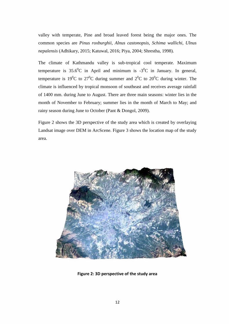
valley with temperate, Pine and broad leaved forest being the major ones. The

common species are Pinus roxburghii, Alnus castonopsis, Schima wallichi, Ulnus

nepalensis (Adhikary, 2015; Katuwal, 2016; Piya, 2004; Shrestha, 1998).

The climate of Kathmandu valley is sub-tropical cool temperate. Maximum

temperature is 35.60C in April and minimum is -3

0C in January. In general,

temperature is 190C to 27

0C during summer and 2

0C to 20

0C during winter. The

climate is influenced by tropical monsoon of southeast and receives average rainfall

of 1400 mm. during June to August. There are three main seasons: winter lies in the

month of November to February; summer lies in the month of March to May; and

rainy season during June to October (Pant & Dongol, 2009).

Figure 2 shows the 3D perspective of the study area which is created by overlaying

Landsat image over DEM in ArcScene. Figure 3 shows the location map of the study

area.

Figure 2: 3D perspective of the study area

13

Kathmandu Valley, Nepal

Study Area

Figure 3: Location map of the study area

14

3. RESEARCH METHODS

This section deals with the various approaches applied to fulfill the aforementioned

aim and objectives. These approaches illustrate the practical implications of GIS and

Remote Sensing in relation to the use of spatial-temporal datasets to address real

world problems, the UHI phenomenon in our case. The major methods used in our

research are supervised maximum likelihood classification, change detection

analysis, urban fragmentation, hot spot analysis and regression analysis.

3.1 Supervised Maximum Likelihood Classification

Supervised Maximum Likelihood Classification was used to classify the study area

into land use land cover classes. In this method, the spectral characteristics of the

classes were defined by identifying training samples. Knowledge about the area of

interest played a vital role in this process. After the collection of training samples,

image classification was carried out by applying the Maximum Likelihood

Classification algorithm. The algorithm assigns a cell to the class of the highest

probability, whereby the probability value is the statistical distance based on the

mean values and covariance matrix of the clusters (Tempfli, 2009).

At least 50 pixels in an average were taken from spectrally enhanced images for each

class as training samples. Color composites based on band combinations - 5, 4, 3 in

Landsat 8 and 4, 3, 2 in Landsat 5 TM were created to enhance image interpretation.

Likewise high resolution IKONOS images, digital Orthophotos and digital

topographic maps were also used as reference. The classification result included six

land use land cover classes: Urban, Agriculture, Forest, Bare soil, Open area and

Water. These classes were in accordance to the existing practices in the Kathmandu

valley as well as the system adopted by the Survey Department of Nepal. Urban area

covered built up areas comprising buildings, roads, airport runway and other

impervious surfaces. Agriculture represents cropland while bare soil means clear

exposed surfaces such as preconstruction areas, river banks not covered by the

vegetation etc. Lands with little vegetation cover were classified as Open area. In this

15

way the final land use land cover maps were produced for all three years 1988, 2000

and 2014 respectively. These maps enabled spatial-temporal change analysis.

3.2 Accuracy Assessment

Usually LULC maps derived from classification contain some errors due to several

factors that range from the initial data acquisition procedure to the implementation of

the classification technique. Thus accuracy assessment of classification results is

mandatory. The most common method generally used for the accuracy assessment is

the error matrix (confusion matrix). An error matrix is an arrangement of numbers

representing number of samples assigned to a specific category relative to the ground

truth, in rows and columns. The rows in the matrix represents classification derived

LULC maps while columns represent reference data collected from the field work.

This matrix enables computation of several statistical measures such as overall

classification accuracy, error of omission and commission, and kappa coefficient

(Congalton and Green, 1999).

Overall accuracy is defined as the ratio of the number of correctly classified pixels

(i.e. the sum of the diagonal elements) to the total number of pixels checked,

expressed in percentage. However, overall accuracy is an average, so it does not

reveal how error is distributed between the classes. Therefore, other measures like

error of omission and error of commission were introduced. Error of omission is the

percentage of pixels that should have been put into a given category but were not.

Error of commission is the percentage of pixels placed in a given category when they

actually belong to the other category. Error of omission corresponds to Producer’s

accuracy and error of commission corresponds to User’s accuracy. Thus Producer’s

accuracy represents the percentage of a given category correctly identified on the

map and User’s accuracy represents the probability that the given pixel will appear

on the ground as it is categorized. The kappa statistics reflects the difference between

actual agreement and the agreement expected by chance. It incorporates the off

diagonal elements of the error matrix (Foody, 2002; Lillesand et al., 2007; Tempfli,

2009).

16

The Kappa coefficient was calculated according to the equation (1) given by

Congalton and Green (1999):

∑

∑

∑

(1)

where,

r = no. of rows in the error matrix

Xii = no. of observations in row i column i (along the diagonal)

Xi+ = marginal total of row i (right of the matrix)

X+i = marginal total of column i (bottom of the matrix)

N = total no. of observations in the matrix

For the accuracy assessment of our classification results, 250 random points were

taken from the classified image to compare with high resolution IKONOS images

and digital Orthophotos. Based on this, we calculated the Overall accuracy, User’s

accuracy, Producer’s accuracy and Kappa index to evaluate the classification

accuracy.

3.3 Land Surface Temperature Retrieval

Land surface temperature was retrieved from the thermal infrared band of Landsat

images (band 6 of Landsat TM 5 and band 10 of Landsat 8). The basic steps for the

retrieval of LST given below are based on the guidelines provided in Landsat Data

Users Handbook published by USGS (Landsat 7, 2011; Landsat 8, 2015). Besides,

one of the methods discussed in the research article by Giannini et al. (2015) has

been also taken as reference.

i. Conversion of pixel values to radiance

The pixel values from digital number units were converted into radiance

using the header files parameters of Landsat images as follows:

17

For Landsat TM 5:

Lλ = Grescale * QCAL + Brescale (2)

which can be also expressed as:

Lλ =

* (QCAL - QCALMIN + LMINλ

For Landsat 8:

Lλ = ML* QCAL + AL (3)

ii. Atmospheric correction

Removal of atmospheric effects from the thermal bands is essential to

convert radiance to reflectance measures. Therefore, a specific

atmospheric correction model called DOS-1 has been considered in this

study. DOS-1 is applicable to multispectral image data only, and is

explicitly an image based procedure, which means it does not require in

situ measurements. DOS-1 model corrects for both atmospheric additive

scattering component, attributed to path radiance and solar effects - solar

irradiance and solar zenith (Chavez, 1996).

iii. Conversion of spectral radiance to at-sensor brightness temperature

TB

(4)

iv. Determination of emissivity

The correct determination of surface temperature is constrained to an

accurate knowledge of surface emissivity. The emissivity of a surface can

be determined as the contribution of the different components that belong

to the pixels according to their proportions (Synder et al., 1998). In this

study we used NDVI threshold method to determine emissivity as

proposed by Sobrino, Jiménez-Muñoz & Paolini (Sobrino et al., 2004).

However, NDVI is calculated from the reflectance values of the visible

and near infrared bands as follows:

18

NDVI

(5)

where, and are the reflectance obtained by applying the DOS-

1 method as mentioned above, at the Near Infrared band and Red band,

for atmospheric effect correction.

v. Land Surface Temperature retrieval

The land surface temperature corrected for spectral emissivity is

computed as follows (Artis & Carnahan, 1982):

LST

(

) (6)

where,

λ is the central band wavelength of emitted radiance (11.45 µm)

ρ = h * c/ σ (1.438*10-2

m*K) with: h is the Planck’s constant

(6.62* 10-34

J*s),

c is the velocity of the light (2.998*108 m/s) and

σ is the Boltzmann constant (1.38*10-23 J/K)

vi. Convert land surface temperature value from Kelvin unit to degree

Celsius

LST (0Celsius) = LST (Kelvin) – 273.15 (7)

Table 2 below defines all the parameters introduced above.

19

Table 2: Parameters in LST Retrieval

Parameters Definition

Lλ

Grescale

Brescale

QCAL

LMINλ

LMAXλ

QCALMIN

QCALMAX

ML

AL

K1, K2

the spectral radiance at the sensor’s aperture

the rescaled gain (the data product "gain" contained in the

Level 1 product header or ancillary data record)

the rescaled bias (the data product "offset" contained in the

Level 1 product header or ancillary data record )

the quantized calibrated pixel value

the spectral radiance that is scaled to QCALMIN

the spectral radiance that is scaled to QCALMAX

the minimum quantized calibrated pixel value (corresponding

to LMINλ)

the maximum quantized calibrated pixel value

(corresponding to LMAX λ)

the radiance multiplicative scaling factor for the band

(RADIANCE_MULT_BAND_n from the metadata)

the radiance additive scaling factor for the band

(RADIANCE_ADD_BAND_n from the metadata)

the calibration constants

the emissivity of the surface

3.4 Land use Land Cover Indices

NDVI (Normalized Difference Vegetation Index), NDBI (Normalized Difference

Built-up Index) and NDWI (Normalized Difference Water Index) indices were used

to determine the relationship between LULC and LST. These indices can be useful to

assess and monitor the urban thermal environment. Some of these indices were even

used to delineate LULC types based on the appropriate threshold values. Besides

LULC indices, DEM was also used in the analysis. DEM of the study area was

generated based on the contour lines available at 20 meters interval and spot heights.

LULC indices were extracted from the satellite images based on the following

expressions:

20

NDVI = (NIR – R) / (NIR + R) (Rouse et al., 1974) (8)

NDBI = (MIR – NIR) / (MIR + NIR) (Zha et al., 2003) (9)

NDWI = (G – MIR) / (G + MIR) (Xu, 2006) (10)

where, G, R, NIR, MIR are Green, Red, Near Infrared and Mid – infrared bands

respectively.

3.5 Regression Analysis

3.5.1 Linear Regression

We applied multiple linear regression analysis to determine the relationship between

LST and LULC. A multiple linear regression analysis is the statistical process useful

for estimating the relationships among multiple explanatory variables (independent

variables) and a predictor (dependent variable). It is the generalization of linear

regression to multiple variables which can be expressed as (Higgins, 2005):

Yi = β0 + β1Xi1 + β2Xi2 + ………..+ βrXir + ⋴i (11)

where, we consider n no. of observations of one predictor and r explanatory

variables.

Yi = ith

observation of the predictor

Xij = ith

observation of the jth

explanatory variable (j = 1, 2, 3…, r)

βj = parameters to be estimated

⋴i = ith

independent identically distributed normal error

We extracted LST and LULC indices – NDVI, NDBI, NDWI, and DEM for each

pixel in the study area. Three thousand random points were obtained from the LST

image and their corresponding LULC indices values were extracted in ArcGIS to use

them in the linear regression model. Such model gives us a general idea about the

relationship between LST and LULC. However we applied a non-linear regression

method called Kernel Ridge Regression (KRR) to determine the predicted value of

LST because this method is better and more flexible when many explanatory

21

variables are taken into account (Saunders et al., 1998). We used many LULC

variables which may create non-linear correlations; therefore KRR would be suitable

for our purpose.

3.5.2 Non-linear Regression

Ridge Regression technique is especially designed to deal with multi-collinearity or

non-linear dependence of regressors (Rosipal & Trejo, 2001). It is a generalization of

least square regression. For example, in case of linear regression, let us assume that

the aim is to fit the linear function to our training set {( ) (

)}

where T is the no. of examples, is a vector in Rn (n is no. of attributes) and

⋴ R, t

= 1,2,…,T. Least square recommends assessing which minimizes:

∑ ( )

(12)

and using for labeling future examples: if a new example has attributes then the

predicted label will be .

Ridge regression slightly modifies this equation to:

‖ ‖ + ∑ ( )

(13)

where, is a fixed positive constant.

There are different ways to obtain the { } parameters. One of them is applying

constrained minimization methods to the so-called “dual version” of equation (13). In

this case, the estimation depends on the dot products of the elements, i. e. .

KRR is a modification of equation (13) in such a way that non-linear functions can

be fitted implicitly. In this case the aim is related to the estimation of a mapping

function which “transforms” the training points to higher dimensional spaces

( ) whereby we can deal with the problem as a linearization of the non-

linear lower dimensional space where the points lie. It can be shown that the dot

products of the elements, i.e., are transformed into ( ) which is

known as “transformation kernel” (Saunders et al., 1998).

22

3.5.3 Experimental setup for the appropriate approach assessment

for LST prediction

In order to determine the appropriate approach between LULC indices and LULC

class for future LST prediction, first of all, we generated training sets for both LULC

indices and LULC class. In case of LULC indices, we obtained training sets as we

discussed previously for the linear regression method. But for the LULC class,

initially we calculated the proportion of each land use land cover class using three

different window sizes: 5 by 5, 10 by 10 and 20 by 20 which means 150 m, 300 m

and 600 m pixel resolution respectively. Then we obtained their corresponding mean

LST values. Zonal statistics tool was used to summarize the value of LST within

each window. After that, we selected three thousand random samples from each of

these three resolutions to generate the training sets for LULC class. Next, we trained

KRR for both LULC class and LULC indices and then validated them on the

corresponding test sets. As per our data, we used LST of 1988 and 2000, and LULC

indices of 2014 to obtain the predicted values of LST in 2014. Similarly for LULC

class, we used LST of 1988 and 2000, and LULC of 2014 for all 5*5, 10*10 and

20*20 window cases to obtain the predicted LST for 2014. Finally we computed

RMSE between measured LST values and predicted LST values in 2014 for all the

training sets of both LULC indices and LULC class to determine the suitable

approach for LST prediction.

3.6 Hot Spot Analysis

Hot Spot Analysis tool in ArcGIS was used to identify statistically significant hot

spots and cold spots from our LST datasets. This tool calculates the Getis-Ord Gi*

statistic given a set of weighted features. Thus the LST raster datasets were

converted to polygon features prior to analysis. The Getis-Ord Gi* Statistics is

defined as:

23

∑ ̅∑

√ ∑

∑

(14)

where, is the attribute value for feature , is the spatial weight between

feature and , is the equal to the total number of features and:

X̅ ∑

(15)

√∑

X̅ (16)

Note: The Gi* statistic is the z-score so no further calculations are required.

The resultant z-score tells whether the features with either high or low values cluster

spatially. A feature with high value may not be statistically significant. To be

statistically significant a feature should have a high value and be surrounded by other

features with high values as well. Besides z-score the output feature class also

contained p-value and confidence level bin (Gi_Bin). A high z-score and small p-

value for a feature would indicate spatial clustering of high values. On the other

hand, a low negative z-score and a small p-value would indicate spatial clustering of

low values (ESRI, 2016). On the basis of Gi_Bin, we categorized LST classes as

very hot spot, hot spot, warm spot, not significant, cool spot, cold spot and very cold

spot.

24

3.7 Urban Fragmentation

As our research focuses on urban growth, the study of urban fragmentation is

relevant. Urban fragmentation helps us to understand the urban landscape, so this

research analyses the spatial-temporal dynamics of urban fragmentation in the study

area. Fragmentation metrics proposed by Angel et al. (2012) have been used in our

study. They are as follows:

Infill: It is a new development that has occurred between two time periods within the

urbanized open space of the earlier period, excluding exterior open space;

Extension: A kind of development between two time periods in contiguous clusters

that contained exterior open space in the earlier period and that were not infill;

Leapfrog: All new construction that occurred between two time periods in the open

countryside, entirely outside of the exterior open space of the earlier period;

The terminologies introduced in the above metrics are defined as follows:

Fringe open space: It consists of all pixels within 100 meters of urban and sub urban

pixels;

Captured open space: It consists of all open space clusters that are fully surrounded

by built up and fringe open space pixels and are less than 200 hectares in area;

Exterior open space: It consists of all fringe open space pixels that are less than 100

meters from the open countryside;

Urbanized open space: It consists of all fringe open space, captured open space and

exterior open space pixels in the city;

Urban built-up pixels: Pixels which have more than 50 percent of built-up pixels

within their walking distance circle;

Suburban built-up pixels: Pixels which have 10-50 percent of built-up pixels within

their walking distance circle;

25

Rural built-up pixels: Pixels which have less than 10 percent of built-up pixels

within their walking distance circle;

Walking distance circle: It is a circle with an area of 1 km2 around a given built-up

pixel.

We applied Urban Landscape Analysis tool, developed by CLEAR, University of

Connecticut (http://clear.uconn.edu/tools/ugat/index.html) to determine the spatial-

temporal dynamics of urban fragmentation. The tool classifies urban area into Urban

built-up, Suburban built-up, Rural built-up, Urbanized open land, Captured open land

and Rural open land, based on spatial density of built-up area. In addition, the tool

also classifies the new development, which has occurred between two consecutive

time periods, as infill, extension and leapfrog, based upon its proximity to the

previously existing development.

26

4. RESULTS & DISCUSSION

4.1 Land use land cover change in the study area

Table 3 summarizes the overall accuracy, user’s accuracy, producer’s accuracy and

kappa coefficient of LULC classification accuracy assessment for the years 1988,

2000 and 2014.

Table 3: Accuracy Assessment of classified images for different years

LULC types

1988 2000 2014

User Ac. Pro Ac. User Ac. Pro Ac. User Ac. Pro Ac.

Urban 86.11 83.78 93.10 81.81 90.00 87.50

Agriculture 87.23 87.23 89.09 87.50 76.60 82.00

Forest 91.22 89.65 92.10 94.59 91.66 91.66

Open area 76.59 83.72 87.87 81.69 75.00 83.34

Bare soil 81.08 78.94 77.77 90.32 85.71 88.23

Water 92.30 88.88 80.76 95.45 95.00 88.36

Overall Ac. 85.60 87.20 88.00

Kappa stat. 0.82 0.84 0.85

Note: User Ac. = User’s Accuracy Pro. Ac. = Producer’s Accuracy

Overall Ac. = Overall Accuracy Kappa stat. = Kappa Coefficient

Therefore, the overall accuracies for the years 1988, 2000 and 2014 were 85.60 %,

87.20 % and 88 % respectively. Forest and Water got the maximum accuracy in all

three years. Meanwhile, Open area got the minimum accuracy. The kappa

coefficients for the classification images were 0.82, 0.84 and 0.85 respectively.

Based on the supervised maximum likelihood classification technique as discussed in

the methodology section, LULC maps were obtained for all three years and then area

estimates and change statistics were computed. Figures 4-6 show the LULC maps for

the year 1988, 2000 and 2014 respectively.

27

LAND USE MAP

Kathmandu Valley Nepal, 1988

Scale 1:180000

Figure 4: Land use land cover map of study area in 1988

28

LAND USE MAP

Kathmandu Valley Nepal, 2000

Scale 1:180000

Figure 5: Land use land cover map of study area in 2000

29

LAND USE MAP

Kathmandu Valley Nepal, 2014

Scale 1:180000

Figure 6: Land use land cover map of study area in 2014

30

Table 4 summarizes the area estimates for the land use land cover classes of the

study area derived from the classification results. Among all LULC types, Open area

constituted the predominant type of land cover in all three years occupying 42.59

percent of the total area in 1988, 45.25 in 2000 and 33.64 in 2014. Agriculture is the

second largest land use type covering 19.85 percent of the total area in 1988, 19.72 in

2000 and 21.61 in 2014. Bare soil follows Agriculture accounting for 15.38 percent

of the total area which is approximately 1 percent greater than that of Forest in 1988.

However, Forest precedes Bare soil by almost two folds in the succeeding years.

Water constitutes the lowest land cover, which is around 2 percent of the total area.

Urban shows dramatic increase in area from 5.75 percent in 1988 to 20.63 percent in

2014.

Table 4: Area statistics of land use land cover classes for 1988 to 2014

LULC 1988 2000 2014

Area (ha) % Area (ha) % Area (ha) %

Urban 2436.64

5.75 4207.63 9.93 8736.38

20.63

Agriculture 8406.26

19.85 8351.02

19.72 9154.87

21.61

Forest 6036.09

14.25 6049.84

14.28 6140.14

14.50

Open area 18040.71

42.59 19168.08

45.25 14249.17

33.64

Bare soil 6513.9

15.38 3731.98

8.81 3279.06

7.74

Water 922.16

2.18 847.21

2.00 796.14

1.88

Figure 7 is the graphical representation of area statistics of land use land cover

classes presented in the Table 4 above. The graph demonstrates that Open area is the

major LULC type. Water occupies the small proportion of the total area. There is a

significant increase in the Urban while opposite trend can be seen for Bare soil and

Open area. Water and Forest observed slight changes during the study period.

31

Figure 7: Land use land cover areas in different years

Likewise, Figures 8-10 and Table 5 illustrate the changes in all LULC types from

1988 to 2014. Table 5 shows the numerical change in area of all LULC types in

terms of hectare and percentage with respect to that of corresponding LULC types in

the previous year, whereas Figures 8-10 show the percentage change in area with

respect to that of the given year graphically.

Table 5: Land use land cover change during 1988 - 2014

LULC 1988 – 2000 2000 - 2014 1988 – 2014

Area (ha) % Area (ha) % Area (ha) %

Urban 1770.99

72.68 4528.75

107.63 6299.74

258.54

Agriculture -55.24

-0.66 803.85

9.62 748.61

8.90

Forest 13.75

0.23 90.3

1.49 104.05

1.72

Open area 1127.37

6.25 -4918.91

-25.66 -3791.54

-21.02

Bare soil -2781.92

-42.71 -452.92

-12.14 -3234.84

-49.66

Water -74.95

-8.13 -51.07

-6.01 -126.02

-13.66

32

During the first period (1988-2000) the land use change is characterized by abrupt

rise in Urban area by approximately 73%. On the other hand Bare soil decreased by

43%. Open area increased by 6% whereas Water decreased by 8%. However there is

no significant change in Forest and Agriculture.

Figure 8: Percentage change in LULC between 1988 and 2000

Figure 9: Percentage change in LULC between 2000 and 2014

33

In the second period (2000-2014), Urban increased sharply by approximately 108%.

Open area showed an opposite trend in this period as compared to the first period

with area declining by 26%. For Bare soil the declining trend reduced sharply from -

43% to -12% in this period. Forest and Water maintained the same trend as that of

the first period. Agriculture showed a sudden growth by 10%, though the changing

trend was insignificant in the first period.

This period (1988-2014) is in fact the overall change from the first and the second

period. There is extreme increment in Urban land use by approximately 259% while

Agriculture showed a nominal increment by 9%. Bare soil, Open area and Water

were reduced by 50%, 21% and 14% respectively. Forest showed negligible

increment of 2% over the period of 26 years.

Figure 11 demonstrates urban growth during different time periods: 1988 – 2000,

2000 – 2014 and 1988 – 2014. Urban growth has been categorized into three classes:

infill, extension and leapfrog. From these maps, it can be clearly seen that extension

type of growth was greater towards the north. This is due to the fact that lands on the

Figure 10: Percentage change in LULC between 1988 and 2014

34

other directions especially to the west are comparitively less accessible, undulating

and difficult to develop (Thapa, 2009). Table 6 summarizes the proportion of urban

growth types during different periods. The table shows that extension type of growth

was dominant in all periods, whereas infill and leapfrog types of growth were

comparitively low.

Figure 11: Urban growth types in different periods

35

Table 6: Proportion of various urban growth types in different periods (%)

Urban Growth type

Different Periods

1988 - 2000 2000 - 2014 1988 – 2014

Infill 18.32 10.85 8.72

Extension 67.90 82.22 84.19

Leapfrog 13.78 6.93 7.09

Apart from urban growth types, we also obtained urban landscape classes to analyze

the impact of different levels of urbanization. Five classes: urban built-up, suburban

built-up, rural built-up, urbanized open land and rural open land were mapped for

urban landscape (Figure 12). Table 7 shows the proportion of urban landscape

classes for different years. There is a gradual increment in urban built-up area at the

expense of rural open land.

Figure 12: Urban landscape classes for different years

36

Table 7: Proportion of various urban landscape types in different years (%)

Urban landscape 1988 2000 2014

Urban built-up 4.50 6.55 18.16

Suburban built-up 2.91 2.82 4.02

Rural built-up 0.54 0.55 0.37

Urbanized open land 1.58 1.86 4.23

Rural open land 90.46 88.22 73.21

4.2 Spatial pattern of LST and LULC indices

4.2.1 Land Surface Temperature

Figure 13 shows the LST maps of the study area in 1988, 2000 and 2014. LST

ranged from 13.960C to 36.77

0C in 1988, 15.84

0C to 39.17

0C in 2000 and 16

0C to

33.980C in 2014. The maximum temperature increased by around 3

0C during 1988 to

2000 and then declined sharply in the year 2014 by around 60C. However, there is a

gradual increase in the minimum temperature in the subsequent years. The sudden

fall in the maximum temperature during 2000 to 2014 can be reasonable, as some

days of the year in the past can be hotter despite of the influence of urban warming

phenomenon caused by urban growth over time. LST pattern analysis indicates low

temperature represented by blue tone at the edges in all maps that stands for the

forest area. High LST represented by a red patch in the middle represents the

impervious surface of the airport and the red patches at the edges represent bare soil

and even rocks in the high cliffs. The central yellow region represents the urban area.

At meticulous observation of the pattern, gradual removal of blue tone in the middle

and formation of uniform yellow tone can be seen, which gives the impression of the

UHI formation.

37

Figure 13: LST of the study area for the years 1988, 2000 and 2014

Figure 14 shows the mean LST within each LULC class in the study area. Forest LULC

type got the minimum mean LST values in all three years (19.910C in 1988, 21.96 in

2000 and 20.58 in 2014) which is even lower than Water (21.52 in 1988, 23.99 in 2000

and 23.56 in 2014). Bare soil got the maximum mean LST values in all three years

(29.10 in 1988, 30.84 in 2000 and 28.93 in 2014). After Bare soil, Urban area got the

highest mean LST values (26.97 in 1988, 28.63 in 2000 and 28.08 in 2014). The mean

LST for Open area is 25.16 in 1988, 27.59 in 2000 and 26.37 in 2014. Similarly the

mean LST value for Agriculture is 22.93 in 1988, 26.83 in 2000 and 25.66 in 2014. In

this way, Forest and Water received low mean LST values, Agriculture and Open area

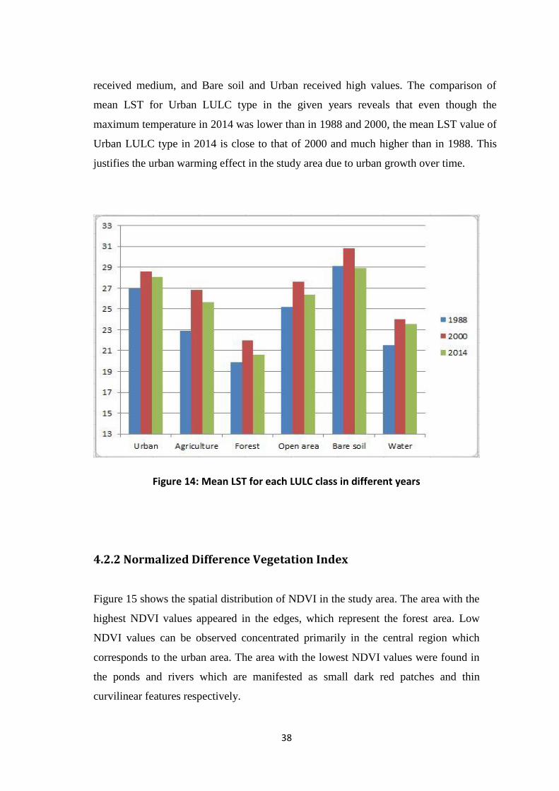
38

received medium, and Bare soil and Urban received high values. The comparison of

mean LST for Urban LULC type in the given years reveals that even though the

maximum temperature in 2014 was lower than in 1988 and 2000, the mean LST value of

Urban LULC type in 2014 is close to that of 2000 and much higher than in 1988. This

justifies the urban warming effect in the study area due to urban growth over time.

Figure 14: Mean LST for each LULC class in different years

4.2.2 Normalized Difference Vegetation Index

Figure 15 shows the spatial distribution of NDVI in the study area. The area with the

highest NDVI values appeared in the edges, which represent the forest area. Low

NDVI values can be observed concentrated primarily in the central region which

corresponds to the urban area. The area with the lowest NDVI values were found in

the ponds and rivers which are manifested as small dark red patches and thin

curvilinear features respectively.

39

Figure 15: NDVI within each LULC class in 1988, 2000 and 2014

Figure 16 shows the bar chart of Mean NDVI values for each LULC class. The

LULC class with the highest mean NDVI value is Forest with NDVI ranging from

0.45 to 0.30 for 1988 to 2014. The other LULC class with high NDVI value is

Agriculture (0.24 to 0.37). Forest and Agriculture showed high NDVI values due to

the dominance of vegetated cover. The lowest mean NDVI is for Water (-0.02 to

0.018) since water lacks vegetation. However it can be seen that its value tends to be

positive over time and the possible reason might be due to the vegetation growth in

water with increasing pollutants. NDVI value for the Open area is approximately

around 0.2 while NDVI value for both urban and Bare soil is around 0.1.

40

4.2.3 Normalized Difference Built-up Index

NDBI maps (Figure 17) revealed an opposite pattern to the NDVI maps in the sense

that Forest, Agriculture and other vegetated areas with high NDVI values received

low NDBI values. Likewise urban area with low NDVI received high NDBI value.

The lowest NDBI is possessed by Water while the highest value is possessed by Bare

soil. In general, built up areas have higher reflectance in relation to MIR band and is

thus expected to have higher NDBI but some studies show that reflectance for certain

types of vegetation increases as water content decreases (Cibula et al., 1992; Gao,

1996). The drier vegetation can even have higher reflectance to MIR resulting in

higher NDBI (Gao, 1996). Therefore, considering dry vegetation in barren land in

higher hills and possibly due to soil characteristics in low land, bare soil areas

exhibited higher NDBI values.

Figure 16: Mean NDVI values for each LULC class in 1988, 2000 and 2014

41

Figure 17: NDBI within each LULC class in 1988, 2000 and 2014

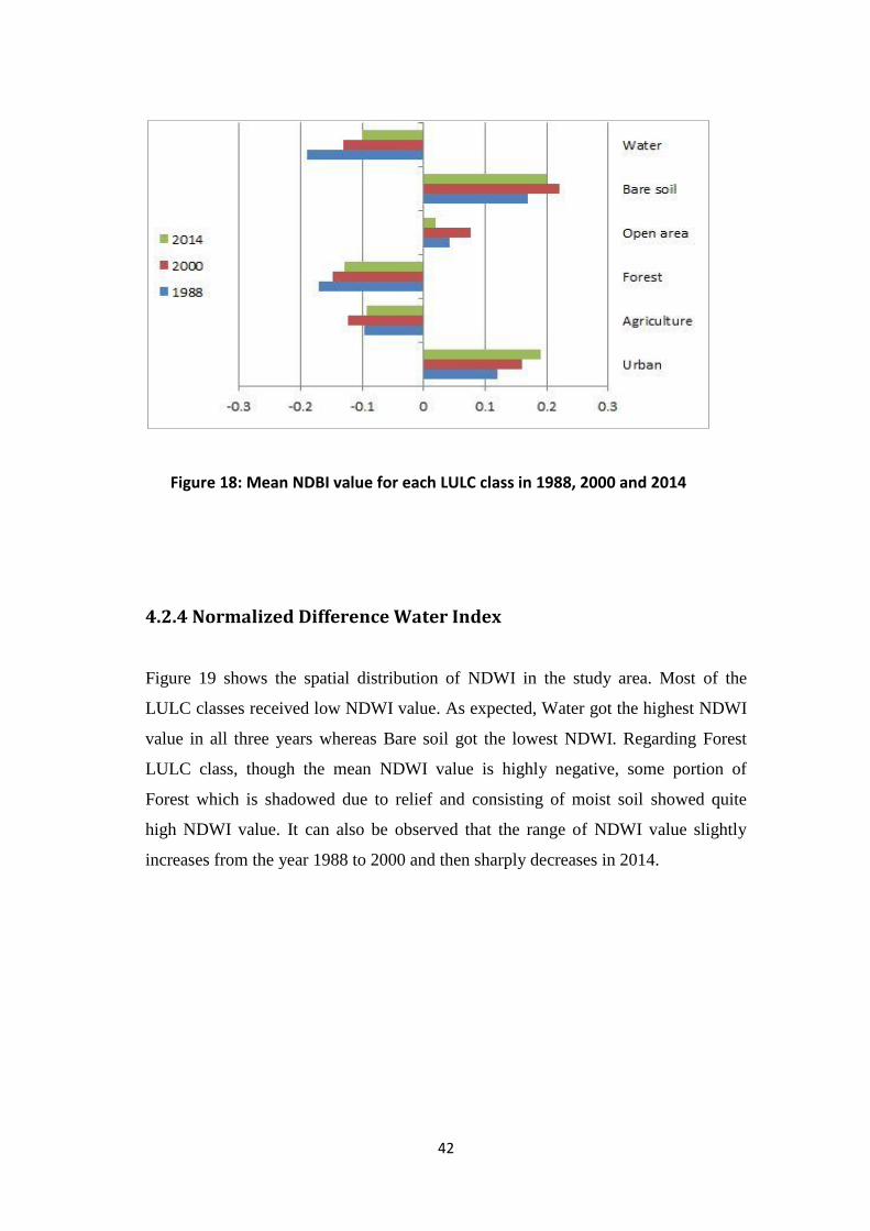
Figure 18 shows the graph of mean NDBI within each LULC class for 1988, 2000

and 2014. In general the NDBI values were low for most of the LULC classes. Water

has the lowest NDBI value (-0.10 to -0.19). After Water, Forest and Agriculture have

the low NDBI values (-0.17 to -0.09). Open area also shows quite low NDBI value

(0.01 to 0.04). On the other hand, Bare soil and Urban LULC classes have

substantially high NDBI values ranging from 0.12 to 0.22.

42

4.2.4 Normalized Difference Water Index

Figure 19 shows the spatial distribution of NDWI in the study area. Most of the

LULC classes received low NDWI value. As expected, Water got the highest NDWI

value in all three years whereas Bare soil got the lowest NDWI. Regarding Forest

LULC class, though the mean NDWI value is highly negative, some portion of

Forest which is shadowed due to relief and consisting of moist soil showed quite

high NDWI value. It can also be observed that the range of NDWI value slightly

increases from the year 1988 to 2000 and then sharply decreases in 2014.

Figure 18: Mean NDBI value for each LULC class in 1988, 2000 and 2014

43

Figure 19: NDWI within each LULC class in 1988, 2000 and 2014

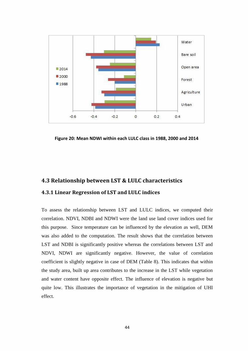
Figure 20 is a bar chart showing mean NDWI value within each LULC class for the

years 1988, 2000 and 2014. As observed, Water is the only LULC class with positive

NDWI value ranging from 0.15 to 0.22. Bare soil, Urban and Open area

demonstrated highly negative NDWI (-0.19 to -0.42). Forest and Agriculture are the

next LULC classes with lower NDWI value after them.

44

4.3 Relationship between LST & LULC characteristics

4.3.1 Linear Regression of LST and LULC indices

To assess the relationship between LST and LULC indices, we computed their

correlation. NDVI, NDBI and NDWI were the land use land cover indices used for

this purpose. Since temperature can be influenced by the elevation as well, DEM

was also added to the computation. The result shows that the correlation between

LST and NDBI is significantly positive whereas the correlations between LST and

NDVI, NDWI are significantly negative. However, the value of correlation

coefficient is slightly negative in case of DEM (Table 8). This indicates that within

the study area, built up area contributes to the increase in the LST while vegetation

and water content have opposite effect. The influence of elevation is negative but

quite low. This illustrates the importance of vegetation in the mitigation of UHI

effect.

Figure 20: Mean NDWI within each LULC class in 1988, 2000 and 2014

45

Table 8: Correlations between LST and LULC indices and DEM

April 3, 1988

LST NDVI NDBI NDWI DEM

LST 1.000 -0.716 0.822 -0.734 -0.219

NDVI -0.716 1.000 -0.897 0.502 0.279

NDBI 0.822 -0.897 1.000 -0.819 -0.169

NDWI -0.734 0.502 -0.819 1.000 -0.009

DEM -0.219 0.279 -0.169 -0.009 1.000

April 4, 2000

LST NDVI NDBI NDWI DEM

LST 1.000 -0.718 0.806 -0. 564 -0.325

NDVI -0.718 1.000 -0.884 0.278 0.459

NDBI 0.806 -0.884 1.000 -0.658 -0.301

NDWI -0.564 0.278 -0.658 1.000 -0.048

DEM -0.325 0.459 -0.301 -0.048 1.000

April 11, 2014

LST NDVI NDBI NDWI DEM

LST 1.000 -0.742 0.839 -0. 570 -0.669

NDVI -0.742 1.000 -0.805 0.238 0.533

NDBI 0.839 -0.805 1.000 -0.747 -0.485

NDWI -0.570 0.238 -0.747 1.000 0.205

DEM -0.669 0.533 -0.485 0.205 1.000

A multiple regression between LST and the indices was then generated for each year,

which is assumed to be useful for monitoring the thermal environment based on

LULC and terrain. The regression models developed in the study are defined below:

LST = -14.79NDVI + 5.40NDBI - 22.56NDWI - 0.001DEM + 22.02 (1988)

LST = -6.70NDVI + 7.47NDBI - 9.69NDWI - 0.001DEM + 24.81 (2000)

LST = -11.80NDVI + 6.99NDBI – 11.08NDWI - 0.004DEM + 33.02 (2014)

where, the unit of LST is degree Celsius, and the unit of DEM is meters.

46

Table 9 shows the coefficients, standard error, t statistic, P-value and coefficient of

determination (R2). The high value of coefficient of determination for all three years

indicates strong linear relationship of the regression models in general. Moreover, P-

value for all predictors in all cases approximately equal to zero indicates that the

predictors are meaningful additions to the generated models. In 1988, high

magnitude of coefficients of NDVI and NDWI indicates their greater contribution to

LST. In 2000, the contribution of NDVI, NDBI and NDWI are almost in the similar

magnitude. However, the contribution of NDVI and NDWI are slightly greater than

NDBI in 2014. The contribution of DEM in all three years is low in comparison to

the LULC indices.

Table 9: Regression Analysis Parameters

April 3, 1988

Estimate Std. error t value P value R2

Constant 22.02 0.24 90.01 0.00 0.71

NDVI -14.79 1.38 -10.69 0.00

NDBI -5.40 1.66 -3.25 0.00

NDWI -22.56 1.47 -15.28 0.00

DEM -0.001 0.00 -9.95 0.00

April 4, 2000

Estimate Std. error t value P value R2

Constant 24.81 0.25 98.10 0.00 0.67

NDVI -6.70 1.05 -6.35 0.00

NDBI 7.47 1.23 6.05 0.00

NDWI -9.69 1.03 -9.32 0.00

DEM -0.001 0.00 -7.94 0.00

April 11, 2014

Estimate Std. error t value P value R2

Constant 33.02 0.17 192.89 0.00 0.80

NDVI -11.80 1.35 -8.72 0.00

NDBI 6.99 1.59 4.38 0.00

NDWI -11.08 1.41 -7.84 0.00

DEM -0.004 0.00 -34.56 0.00

47

To verify the developed regression models graphically, we plotted scatterplot of the

measured (original) LST against estimated LST obtained from the model. Figure 21

shows the scatterplots for the three different years where it can be seen that the points

tend to cluster in the linear fashion in the central region of the plot. The points are

highly clustered in the year 2014 in comparison to the rest of the years. Therefore

considering determination coefficient and visual examination of the scatterplot, the

models seem to be satisfactory.

Figure 21: Measured LST vs Estimated LST for developed regression models

Measured

Esti

mat

ed

Es

tim

ate

d

Year 2014

Esti

mat

ed

Measured

Measured

Year 2000

Year 1988

48

4.3.2 Linear Regression of LST and LULC class

We further developed regression models for each LULC class to understand its

relation to LST comprehensively. Table 10 shows regression models for each LULC

class in the study area for all three years. From the table we can notice that Open area

LULC class has greater coefficient of determination in 1988, Bare soil in 2000 and

Forest in 2014. Water has the lowest coefficient of determination in the year 1988

and 2014. In 2000 Urban LULC class showed the lowest value.

Table 10: Regression equations for each LULC class

April 3, 1988

LULC Regression equations R2

Urban -0.4NDVI + 16.06NDBI + 12.85NDWI + 0.01DEM + 7.74 0.45

Agriculture 4.94NDVI + 12.57NDBI + 3.08NDWI - 0.001DEM + 22.44 0.43

Forest -7.65NDVI - 4.49NDBI - 16.10NDWI - 0.003DEM + 24.10 0.49

Open area -10.27NDVI - 4.78NDBI - 19.68NDWI + 0.004DEM + 13.31 0.59

Bare soil 0.19NDVI + 7.85NDBI - 8.50NDWI + 0.01DEM + 3.39 0.35

Water -6.05NDVI - 2.14NDBI – 3.31NDWI + 0.004DEM + 17.13 0.15

April 4, 2000

LULC Regression equations R2

Urban -16.95NDVI – 7.97NDBI – 7.74NDWI + 0.03DEM – 12.05 0.21

Agriculture 1.72NDVI + 11.49NDBI + 3.90NDWI - 0.006DEM + 16.57 0.36

Forest -13.88NDVI - 15.77NDBI - 25.28NDWI - 0.002DEM + 23.14 0.45

Open area -3.32NDVI + 2.49NDBI – 10.28NDWI + 0.001DEM + 20.76 0.31

Bare soil -10.09NDVI – 2.26NDBI - 18.20NDWI + 0.007DEM + 3.39 0.47

Water -29.44NDVI - 19.12NDBI - 22.64NDWI - 0.004DEM + 31.72 0.38

April 11, 2014

LULC Regression equations R2

Urban -3.54NDVI + 20.33NDBI + 16.58NDWI + 0.007DEM +20.48 0.44

Agriculture -10.55NDVI - 1.58NDBI - 12.10NDWI - 0.002DEM + 29.44 0.39

Forest 1.60NDVI – 1.51NDBI – 15.06NDWI - 0.004DEM + 27.17 0.66

Open area -7.33NDVI + 2.22NDBI – 17.83NDWI - 0.002DEM + 28.49 0.55

Bare soil -3.81NDVI + 4.54NDBI - 8.64NDWI - 0.001DEM + 24.20 0.19

Water -4.69NDVI + 3.90NDBI – 5.39NDWI + 0.002DEM + 23.49 0.13

49

In summary, the relationship between LST and LULC indices varies depending upon

the LULC class. The obtained results showed some anomalies in relation to the

different trends observed for the same LULC class. For instance, NDBI positively

affected LST in 1988 and 2014 for urban LULC class but its effect is negative in

2000. One possible reason might be due to the multi-collinearity effect by the use of

many predictors in the linear regression. Hence we recommend that linear regression

can be useful to explore the general relationship between LST and LULC. However

it may not be always the suitable choice particularly when we are interested to

explore the relationship in depth, considering many LULC variables. Therefore, we

decided to apply Kernel Ridge Regression for further analysis.

4.3.3 Assessment of LULC indices and LULC class based approach for

LST prediction

We commenced our assessment procedure with the linear regression models based

on LULC indices developed in the above section. We used the linear regression

model of the years 1988 and 2000 to generate estimated LST for the consecutive year

2014. Measured LST data of the year 2014 was used as test sample during the

process. Then we computed RMSE between the test sample and estimated LST

obtained from the model as shown in the following table. As the obtained RMSE

values are high, linear regression model seems to be not suitable for the purpose of

use for the LST prediction.

Table 11: RMSE values for LULC indices and linear regression case

Linear Regression Test Sample RMSE

1988 2014 5.49

2000 2014 2.27

After that we switched on to the non-linear Kernel Ridge Regression (KRR). KRR

was trained using the LULC indices and corresponding LST data of the years 1988

and 2000 to produce estimated LST for the consecutive year 2014. Then we

50

computed the RMSE between the test sample and the obtained estimated LST, as

shown in the following table. This time, the obtained RMSE values are better than

the previous ones obtained through the linear regression.

Table 12: RMSE values for LULC indices and KRR case

Training Sample Test Sample RMSE

1988 2014 1.37

2000 2014 1.26

Next we tested LULC class based approach with KRR. As mentioned earlier, we

obtained LST and corresponding LULC proportion data at different window sizes

5*5 10*10 and 20*20. Therefore we computed RMSE values for each window case.

Initially KRR was trained with 1988 and 2000 data. Then we obtained estimated LST

for the year 2014 based on the training samples of 1988 and 2000 for all 5*5, 10*10

and 20*20 window cases. The RMSE was then determined between the test samples

and obtained estimated LST for the year 2014 as follows.

Table 13: RMSE values for LULC class and KRR case

Training Sample Test Sample Window size RMSE

1988 2014 5*5 1.90

1988 2014 10*10 1.86

1988 2014 20*20 1.78

2000 2014 5*5 1.88

2000 2014 10*10 1.54 2000 2014 20*20 1.41

Comparing the RMSE values we can conclude that LULC indices based approach

using recent training sample is more suitable for the future LST prediction of the

study area. Applying KRR for LULC indices of 2000 to predict LST for the year

2014 yielded the lowest RMSE of 1.26 between the test sample and the estimated

LST for that year. Figure 22 depicts the scatterplot between measured and estimated

LST for this particular case.

51

4.4 Impact of urban growth on UHI effect

Getis-ord Gi* Statistics was applied to the LST dataset to detect the presence of hot

or cold spots over the study area. This is considered to be an effective approach to

visualize the effect of urban heat island (Goswami et al., 2013). By this method, we

are concerned with the thermal pattern rather than the absolute value of mean surface

temperature. It should also be noted that the identification of hot or cold spots by this

method does not necessarily imply the mean surface temperature being high or low.

Figure 23 shows the Hot Spot maps of the study area for the three different dates.

Figure 22: Measured LST vs. Estimated LST for LULC indices and KRR case for 2000

Measured

Est

imat

ed

52

Figure 23: Hot Spot Analysis for LST in different years

The maps for the year 1988 and 2000 primarily show heat island in the airport area

and the core urban area. However there is a dramatic change in the year 2014. There

is a formation of big heat island covering almost the whole urban area in that year.

There is a gradual removal of cold region in the central region during the period

1988-2000. The cold region is observed in the areas of high vegetation cover such as

forest, open areas and agriculture. This justifies the importance of vegetation in

minimizing the urban heat island effect.

Tables 14-16 show the percentage distribution of different thermal types over various

LULC classes. In other words, they show the contribution of various LULC types in

the spatial distribution of thermal pattern. Generally cold region is observed to

occupy the greater area than hot region. However in the year 2014, hot region

superseded cold region. Not-significant region also occupies large portion in our

53

study area. Though the contribution of urban area in the very hot region was minimal

in the year 1988 and 2000, it increased by around 8% in the year 2014. Forest and

Agriculture are the coldest LULC types. Figure 24 shows the LULC distribution

specifically in the Hot Spot area that is the area observed to be the hot spot at 99%

confidence level. Dominant land use observed in the Hot Spot area is Open area in

the first two years, but it is superseded by the Urban area in 2014. It can be stated

that the Urban area showed more impact on Hot Spot over time in the study area.

Table 14: Proportion of various thermal region in different LULC in 1988 (%)

LULC Very cold

Cold

Cool

Not Sig. Warm

Hot

Very Hot

Urban 0.328

0.398

0.291

3.913

0.162

0.210

0.447

Agriculture 15.192

1.755

0.737

2.133

0.011

0.009

0.005

Forest 12.345

0.559

0.252

0.998

0.026

0.033

0.034

Open area 5.035

3.020

1.845

20.716

1.335

2.201

8.439

Bare soil 0.305

0.292

0.224

7.206

0.859

1.644

4.844

Water 0.653 0.224 0.133 1.049 0.035 0.032 0.047

Total 33.860 6.251 3.485 36.018 2.431 4.132 13.819

Table 15: Proportion of various thermal region in different LULC in 2000 (%)

LULC Very Cold Cold Cool Not Sig. Warm Hot Very Hot

Urban 0.106 0.127 0.122 6.450 0.642 0.708 1.775

Agriculture 11.416 2.228 1.044 4.837 0.057 0.064 0.068

Forest 13.005 0.445 0.152 0.654 0.009 0.007 0.008

Open area 5.374 2.583 1.693 23.208 1.798 2.730 7.867

Bare soil 0.066 0.072 0.047 2.249 0.433 0.887 5.053

Water 0.537 0.185 0.092 0.962 0.048 0.078 0.095

Total 30.506 5.642 3.152 38.363 2.988 4.476 14.869

54

Table 16: Proportion of various thermal region in different LULC in 2014 (%)

LULC Very cold Cold Cool Not Sig. Warm Hot Very Hot

Urban 0.000 0.0003 0.001 6.129 1.987 4.031 8.475

Agriculture 1.602 2.018 1.287 15.521 0.439 0.460 0.283

Forest 13.713 0.387 0.127 0.264 0.001 0.001 0.0003

Open area 3.332 1.467 0.896 17.350 1.893 3.122 5.579

Bare soil 0.0002 0.005 0.008 1.920 0.599 1.368 3.839

Water 0.014 0.057 0.048 1.073 0.122 0.192 0.371

Total 18.663 3.937 2.370 42.259 5.043 9.175 18.549

a) Year: 1988 b) Year: 2000

c) Year: 2014

Figure 24: LULC distribution (% area) in Hot Spot area

55

We know that urban growth causes urban landscape changes. Therefore it is

important to relate urban landscape to the land surface temperature to understand

how urban fragmentation causes the UHI effect. Table 17 shows that urban built-up

is the hottest landscape type whereas rural open area is the coldest landscape type.

The spatial pattern of LST can be visualized from the table as we transit through the

different zones from the hottest urban built-up landscape type to the coldest rural

open area landscape type, which helps us to visualize the UHI formation in the study

area. Moreover, the lower LST of urbanized open area in comparison to urban built-

up and suburban built-up indicates the importance of open space such as parks and

other recreational areas to minimize the UHI effect.

Table 17: Mean LST by urban landscape in degree Celsius

Urban landscape 1988 2000 2014

Urban built-up 26.92 28.98 28.67

Suburban built-up 26.10 27.89 27.84

Rural built-up 25.90 27.13 26.95

Urbanized open land 25.90 27.56 27.11

Rural open land 24.74 26.19 25.88

Table 18 shows the mean LST for each urban growth type during different

development periods. Infill growth has the maximum mean LST whereas Leapfrog

has the minimum mean LST in all periods. This is because infill area is usually

surrounded by the built-up area itself having high LST value which positively

influences the LST of infill area, while leapfrog area is surrounded by the other

LULC types such as open area, agriculture etc. having low LST value, which

negatively influences the LST of leapfrog area.

56

Table 18: Mean LST by urban growth type in degree Celsius

Urban growth type 1988-2000 2000-2014 1988-2014

Infill 28.00 28.08 28.17

Extension 27.75 27.26 27.51

Leapfrog 27.30 27.04 27.13

To explore the impact of urban growth on land surface temperature, we applied

linear regression to analyze the relationship between urban land cover and surface

temperature. Using zonal statistics tool in ArcGIS we determined the mean LST at

each percentage of urban cover from 0% to 100%. Figure 25 shows the linear

regression models for the three different years. The regression models indicate that

for every 1% increase in urban area, there will be increase in mean LST by 0.0120C

in 1988, 0.0260C in 2000 and 0.039

0C in 2014 respectively.

Figure 25: Linear regression between urban cover and LST

57

5. CONCLUSION

The study revealed high rate of urban growth in Kathmandu valley. The main drivers

of such growth are high population influx and improper land use plan. As a result,

productive agricultural land, open area are being replaced by the concrete structures.

This trend is expected to be more severe in future unless proper land use plans and

policies are implemented. Various types of urban growth such as infill, extension and

leapfrog were found to exist in the valley. However, infill type of urban growth is

more hazardous in the sense that it fills up existing open area making cities

congested and the consequences of such growth were apparent during Nepal

Earthquake 2015, when many people lose their lives due to inaccessibility to the safe

open places for emergency evacuation.

Based on our analysis of thermal pattern of the study area over the given period of

time, we found gradual increase in temperature in urban area. There was the

formation of urban heat island in the central urban area of the valley. The study

proved that the surface temperature is influenced by the urban growth. Urban growth

not only increases the UHI effect but also affects quality of life of the people residing

in the urban area.

We also explored the relationship between LST and LULC through regression

analysis. The results indicated strong linear relationship between surface temperature

and LULC indices. We then performed regression analysis between LST and LULC

indices for each LULC class. This exhibited variations in the relationship depending

upon the LULC types. Regarding determination of the appropriate approach for LST

prediction, we compared LULC indices and LULC class based methods and found

that LULC indices method gives better prediction in comparison.

However there were some limitations in the study. The resolution of the images was

just moderate for classification and change detection purpose. Despite of massive

repository of Landsat imagery, sometimes it is difficult to get the suitable images as

per our requirement. In addition, due to spectral mixing of different land cover within

the pixels and complex landscape of the study area, pixel based classification did not

give us higher accuracy. Likewise our study focused on LST pattern rather than its

58

absolute value over the area of interest. Furthermore, our study is primarily based on

daytime LST during summer season considering only three years.

Hence we recommend that as urban growth in Kathmandu valley is in critical

condition it is high time that concerned authorities take necessary initiatives and

urban residents develop resilience to urban growth and UHI effect. We also

recommend using high resolution images and other classification method so that

more LULC classes at higher accuracy can be obtained. To obtain robust results for

LULC-LST relationship it is better to take into account both daytime and nighttime

temperature data for more years. Similarly, if absolute temperature is also to be

prioritized then atmospheric correction parameters considering local climatic

parameters has to be applied. Last but not the least we need to assess other regression

methods as well to understand the LULC-LST relationship in depth.

59

REFERENCES

ADB/ICIMOD. (2006). Environment Assessment of Nepal: Emerging Issues and

Challenges.Kathmandu: ICIMOD.

Adhikary, D. (2015). 2015 Nepal Earthquake – A Geological and Geotechnical

Perspective and Implications to Kathmandu Valley. Last visit 1/7/2017,

https://dpadhikary.wordpress.com/tag/kathmandu-soil

Ahmed, B., Kamruzzaman, M., Zhu, X., Rahman, M.S., & Choi, K. (2013).

Simulating Land Cover Changes and Their Impacts on Land Surface

Temperature in Dhaka, Bangladesh. Remote Sensing, 5, 5969-5998.

Angel, S., Parent, J., & Civco, D.L. (2012). The fragmentation of urban landscapes:

global evidence of a key attribute of the spatial structure of cities, 1990–2000.

Environment and Urbanization, 24(1), 249-283.

Artis, D.A., Carnahan, W.H. (1982). Survey of emissivity variability in

thermography of urban areas, Remote Sensing of Environment. 12(4), 313–329.

Baniya, N. (2008). Land Suitability Evaluation Using GIS for Vegetable Crops in

Kathmandu Valley/Nepal. Last visit 1/6/2017,

http://edoc.hu-berlin.de/dissertationen/baniya-nabarath-2008-10-

13/PDF/baniya.pdf

Bekele, H. (2005). Urbanization and Urban Sprawl. Master thesis, Department of

Infrastructure Section of Building and Real Estate Economics, Kungliga

Tekniska Högskolan, Stockholm, Sweden.

Central Bureau of Statistics (CBS portal, 2017). http://www.cbs.gov.np

Chavez, P.S. (1996). Image-Based Atmospheric Corrections – Revisited and

Improved, Photogrammetric Engineering & Remote Sensing. 62(9), 1025-1036. Chen, X., Zhao, H., Li, P., & Yin, Z. (2006). Remote sensing image-based analysis

of the relationship between urban heat island and land use/cover changes.

Remote Sensing of Environment, 104(2), 133-146.

Cibula, W.G., Zetka, E.F. & Rickman, D.L. (1992). Response of thematic mapper

bands to plant water stress. International Journal of Remote Sensing, 13, 1869-

1880.

Congalton, R. & Green, K. (1999). Assessing the accuracy of remotely sensed data.

Principles and practices. Lewis Publishers, Boca Raton, Florida.137p.

60

Coseo, P., & Larsen, L. (2015). Cooling the Heat Island in Compact Urban

Environments: The Effectiveness of Chicago's Green Alley Program. Procedia

Engineering, 118, 691-710.

DoR. (2004). List of Important Roads and Status. Road Statistics, Kathmandu:

Government of Nepal. Last visit 1/4/2017,

https://www.dor.gov.np/road_statistic_2004/list_of_important_roads.php

ESRI. (2016). How Hot Spot Analysis (Getis-Ord Gi*) works, Last visit 17/10/2016, http://pro.arcgis.com/en/pro-app/tool-reference/spatial-statistics/h-how-hot-

spot-analysis-getis-ord-gi-spatial-stati.html

Fabrizi, R., Bonafoni, S., & Biondi, R. (2010). Satellite and ground-based sensors for

the urban heat island analysis in the City of Rome. Remote Sensing, 2, 1400–

1415.

Foody, G. (2002). Status of land covers classification accuracy assessment, Remote

Sensing of Environment, 80, 185-201.

Gao, B.C. (1996). NDWI–A normalized difference water index for remote sensing of

vegetation liquid water from space, Remote Sensing of Environment, 58(3),

257–266.

Ghimire A.B., & Upreti, B.R. (2008). Conflict Induced Displacement: An emerging

phenomenon of Internal Migration in Nepal. In Pyakuryal, K.N., Upreti, B.R.,

& Sharma, S.R. (Eds.), Nepal: Transition to Transformation (pp. 101-140).

Kathmandu University: Human and Natural Resources Studies Center &

NCCR North South: South Asia Regional Coordination Office.

Goswami, J., Roy, S., & Sudhakar, S. (2013). A Novel Approach in Identification of

Urban Hot Spot Using Geospatial Technology: A Case Study in Kamrup Metro

District of Assam, Internation Journal of Geosciences, 4, pp. 898-903.

Goward, S.N. (1981). THERMAL BEHAVIOR OF URBAN LANDSCAPES AND

THE URBAN HEAT ISLAND. Physical Geography, 2(1), 19-33.

Grimmond, S. (2007). Urbanization and global environmental change: local effects

of urban warming. The Geographical Journal, 173(1), 83-88.

Guo, G., Wu, Z., Xiao, R., Chen, Y., Liu, X., & Zhang, X. (2015). Impacts of urban

biophysical composition on land surface temperature in urban heat island

clusters. Landscape and Urban Planning, 135, 1-10.

Higgins, J. (2005). The Radical Statistician. Last visit, 1/10/2017,

http://www.biddle.com/documents/bcg_comp_chapter4.pdf

61

Imhoff, M.L., Zhang, P., Wolfe, R.E., & Bounoua, L. (2010). Remote sensing of the

urban heat island effect across biomes in the continental USA. Remote Sensing

of Environment, 114(3), 504-513.

Kathmandu Valley in Nepal. (Tourism portal, 2017).

http://www.welcomenepal.com/places-to-see/kathmandu-valley.html

Katuwal, H.B., Bhandari, J., Thapa, V., Gurung, R., Chaudhary, R., Magar, T.G., &

Chaudhary, H. (2016). How many birds do the sacred forests hold? The Journal

of Zoology Studies, 3(4), 7-19.

Kim, J.P., & Guldmann, J.M. (2014). Land-Use Planning and the Urban Heat Island.

Environmental and Planning B: Planning and Design, 41(6), 1077-1099.

Landsat, N. A. S. A. (7). Science Data Users Handbook. 2011, Last visit 9/23/2016,

http://landsathandbook.gsfc.nasa.gov/inst_cal/prog_sect8_2.html.

Landsat, N. A. S. A. (8). Science Data Users Handbook. 2015, Last visit 10/18/2016

http://landsat.usgs.gov/l8handbook.php.

Li, K., Lin, B., Jiang, D. (2012). A New Urban Planning Approach for Studying Heat

Islands at the Community Level. Journal of Heat Island Institute, 7(2), 50-54.

Lillesand, T., Keifer, R.W., & Chipman, J. (2007). Remote Sensing and Image

Interpretation (Sixth Edition), Wiley, Hoboken, USA.

Lo, C.P., & Quattrochi, D.A. (2003). Land-Use and Land-Cover Change, Urban Heat

Island Phenomenon, and Health Implications. Photogrammetric Engineering &

Remote Sensing, 9, 1053-1063.

Mirzaei, P. A. (2015). Recent challenges in modeling of urban heat island.

Sustainable Cities and Society, 19, 200-206.

Oke, T. R. (1982). The energetic basis of the urban heat island. Quarterly Journal of

Royal Meteorological Society, 108, 1–24.

Pant, P. R., Dongol, D. (2009). Kathmandu Valley Profile, Briefing Paper. Last visit

1/6/2017,

http://www.eastwestcenter.org/fileadmin/resources/seminars/Urbanization_Sem

inar/Kathmandu_Valley_Brief_for_EWC___KMC_Workshop__Feb_2009.pdf

Parker, D. E. (2010). Urban heat island effects on estimates of observed climate

change. Wiley Interdisciplinary Reviews: Climate Change, 1(1), 123–133.

Piya, B.K. (2004). Generation of a Geological database for Liquefaction hazard

assessment in Kathmandu valley. Master thesis, International Institute for Geo-

information Science and Earth Observation, ITC, Enschede, Netherlands.

62

Qin, Z., Karnieli, A., & Berliner, P. (2001). A mono-window algorithm for retrieving

land surface temperature from Landsat TM data and its application to the

Israel-Egypt border region. International Journal of Remote Sensing, 18, 3719-

3746.

Quattrochi, D. A., & Luvall, J. C. (1999). Thermal infrared remote sensing for

analysis of landscape ecological processes: methods and

applications.Landscape ecology, 14(6), 577-598.

Rimal, B. (2011).Urban Growth and Land use/Land cover change of Pokhara Sub-

Metropolitan city, Nepal. Journal of Theoretical and Applied Information

Technology, 26(2), 118-129.

Rizwan, A.M., Dennis, L.Y.C., & Liu, C. (2008). A review on the generation,

determination and mitigation of Urban Heat Island. Journal of Environmental

Sciences, 20(1), 120-128.

Rosipal, R., & Trejo, L.J. (2001). Kernel Partial Least Squares Regression in

Reproducing Kernel Hilbert Space, Last visit 1/10/2017,

http://www.jmlr.org/papers/volume2/rosipal01a/rosipal01a.pdf

Rouse Jr, J., Haas, R. H., Schell, J. A., & Deering, D. W. (1974). Monitoring

vegetation systems in the Great Plains with ERTS. NASA special publication,

351, 309.

Sailor, D. J., & Lu, L. (2004). A top-down methodology for developing diurnal and

seasonal anthropogenic heating profiles for urban areas. Atmospheric

Environment, 38, 2737–2748. Saitoh, T.S., Shimada, T., & Hoshi, H. (1996). Modeling and simulation of the

Tokyo urban heat island. Atmospheric Environment, 30(20), 3431-3442.

Saunders, C., Gammerman, A., & Vovk, V. (1998). Ridge regression learning

algorithm in dual variables. In (ICML-1998) Proceedings of the 15th

International Conference on Machine Learning , 515-521.

Sharma, P. (2003). Urbanization and Development. In Population Monograph of

Nepal (Vol. 1, pp. 375-412). Kathmandu: Central Bureau of Statistics.

Shrestha, T.K. (1998). The Spiny Babbler, R.K Printers, Teku, Kathmandu.

Snyder, W.C., Wan, Z., Zhang, Y., & Feng, Y.Z. (1998). Classification based

emissivity for land surface temperature measurement from space, International

Journal of Remote Sensing. 19 (14), 2753–2774.

63

Sobrino, J. A., Jiménez-Muñoz, J. C., & Paolini, L. (2004). Land surface temperature

retrieval from LANDSAT TM 5. Remote Sensing of environment, 90(4), 434-

440.

SRIVANIT, M., Hokao, K., & Phonekeo, V. (2012). Assessing the Impact of

Urbanization on Urban Thermal Environment: A Case Study of Bangkok

Metropolitan, International Journal of Applied Science and Technology, 2(7),

243-256.

Stewart, I. D., & Oke, T.R. (2012). Local climate zones for urban temperature

studies. American Meteorological Society, 93, 1879–1900.

Sun, Q., Wu, Z., & Tan, J. (2012). The relationship between land surface temperature

and land use/land cover in Guangzhou, China. Environmental Earth Science,

65, 1687-1694.

Tan, J., Zheng, Y., Tang, X., Guo, C., Li, L., Song, G., Zhen, X., Yuan, D.,

Kalkstein, A.J., & Li, F. (2010). The urban heat island and its impact on heat

waves and human health in Shanghai. International Journal of Biometeorology,

54(1), 75-84.

Tempfli, K., Kerle, N., Huurneman, G.C., & Janssen, L.L.F. (2009). Principles of

Remote Sensing. An introductory textbook (ITC Educational Textbook Series

2), Enschede, ITC.

Thapa, R.B. (2009). Spatial Process of Urbanization in Kathmandu Valley, Nepal.

PhD. Thesis, Graduate School of Life and Environmental Sciences, University

of Tsukuba, Tsukuba, Japan.

Thapa, R.B., & Murayama, Y. (2009). Examining Spatiotemporal Urbanization

Patterns in Kathmandu Valley, Nepal: Remote Sensing and Spatial Metrics

Approaches. Remote Sensing, 1, 534-556.

Tran, H., Uchihama, D., Ochi, S., & Yasuoka, Y. (2006). Assessment with satellite

data of the urban heat island effects in Asian mega cities. International Journal

of Applied Earth Observation and Geoinformation, 8(1), 34-48.

UNHABITAT. (2015). Kathmandu Valley, Nepal – Climate Change Vulnerability

Assessment. Last visit 9/11/2016, http://unhabitat.org/books/kathmandu-valley-nepal-climate-change-vulnerability-assessment.

64

United Nations Office of the High Commissioner for Human Rights (UN-OHCHR).

(2012). Nepal Conflict Report. Geneva.

Weng, Q., Lu, D., & Schubring, J. (2004). Estimation of land surface temperature–

vegetation abundance relationship for urban heat island studies. Remote

Sensing of Environment, 89(4), 467-483.

Xu, H. (2006). Modification of Normalised Difference Water Index (NDWI) to

Enhance Open Water Features in Remotely Sensed Imagery. International

Journal of Remote Sensing, 27(14), 3025-3033.

Yu, X., Guo, X., & Wu, Z. (2014). Land Surface Temperature Retrieval from

Landsat 8 TIRS - Comparison between Radiative Transfer Equation-Based

Method, Split Window Algorithm and Single Channel Method. Remote

Sensing, 6, 9829-9852.

Yuan, F., & Bauer, M.E. (2007). Comparison of impervious surface area and

normalized difference vegetation index as indicators of surface urban heat

island effects in Landsat imagery. Remote Sensing of Environment, 106(3),

375-386.

Zaksek, K., & Ostir, K. (2011). Downscaling land surface temperature for urban heat

island diurnal cycle analysis. Remote Sensing of Environment, 115, 114-124.

Zha, Y., Gao, J., & Ni, S. (2003). Use of normalized difference built-up index in

automatically mapping urban areas from TM imagery, International Journal of

Remote Sensing, 24(3), 583–594.

Zhu, S., & Zhang, G. (2011, October). Analysis on Relationship between Urban

Land Surface Temperature and Landcover from Landsat Etm+ Data. In: Proc.

of Fourth International Symposium on Knowledge Acquisition and Modeling,

IEEE, Sanya, China.

65

APPENDICES

1. Band Designations for Landsat 4-5 Thematic Mapper (TM)

(Source: USGS portal)

2. Band Designations for Landsat 8 OLI (Source: USGS portal)

EXPLORING THE IMPACT OF URBAN GROWTH ON LAND SURFACE

TEMPERATURE OF KATHMANDU VALLEY, NEPAL

2017

Sushil Thapa