Exploring the Kinetics of Domain Switching in Ferroelectrics for Structural Applications Thesis by Charles Stanley Wojnar In Partial Fulfillment of the Requirements for the Degree of Doctor of Philosophy California Institute of Technology Pasadena, California 2015 (Submitted June 5, 2015)
Transcript
Exploring the Kinetics of Domain Switching inFerroelectrics for Structural Applications
A.1 Approximate properties of circuit components used and voltages applied in experiments.139
1
Chapter 1
Introduction
The multiscale nature of materials becomes evident upon their observation under the microscope.
In metals, grain and twin boundaries are seen on the micro scale while smaller defects such as dis-
locations, stacking faults, and vacancies are observed on the nano and atomic level. Microstructure
has a significant effect on the macroscopic properties of materials. For example, the interaction of
dislocations and grain boundaries influences the macroscopic yield strength of metals. In other types
of materials such as ceramics, different atomic bonding and crystal (or lack of crystal) structure
generally lead to stiffer and more brittle behavior compared to metals. Thus, tailoring materials to
exhibit desirable mechanical properties requires understanding their microstructure.
The microstructure of materials is normally unchanging. However, the evolution of microstruc-
ture over time (or kinetics) becomes important when materials are subjected to time-varying (dy-
namic) external forces including mechanical, thermal, and electrical loading. For example, cyclic
mechanical loading causes fatigue through microcracking (Alexopoulos et al., 2013), thermal cycling
changes the grain sizes in metals and effects their mechanical properties (Callister and Rethwisch,
2009), and cyclic electrical loading can degrade materials (Wang et al., 2014). The combined effects
of microstructure and dynamic thermo-electromechanical loading clearly present a difficult chal-
lenge for understanding, predicting, and utilizing materials under these conditions. Some of these
effects have been studied extensively, however, there exists a large gap in our understanding for the
case of dynamic electromechanical loading of materials with microstructure evolution. Therefore,
the goal of this thesis research is to investigate this particular piece of the puzzle.
The materials of interest are ferroelectrics. Although most materials are not affected by elec-
tric fields (at least at moderate levels), ferroelectrics are a special class of materials that exhibit
2
electromechanical coupling. Moreover, their electromechanical response is strongly influenced by
their microstructure. Therefore, ferroelectrics present themselves as an ideal material for this study.
While there are many ways dynamic loads are applied to materials, only the case of harmonic (i.e.
cyclic) electromechanical loading will be considered. The response of materials under harmonic
loading will be studied within the framework of viscoelasticity and, in particular, the dynamic stiff-
ness and damping of ferroelectrics will be characterized. Therefore, an introduction to ferroelectric
materials will first be given in Section 1.1. Then, a review of the relevant concepts from viscoelas-
ticity will be presented in Section 1.2. Finally, the motivation for studying the viscoelasticity of
ferroelectrics will be discussed in Section 1.3 and an outline of the thesis is given in Section 1.4.
1.1 Ferroelectrics
The possibility of electromechanical coupling in materials was first discovered by the Polish-French
scientists Pierre and Marie Curie (1880a; 1880b). They observed that an electric field was generated
when a stress was applied to quartz crystals. The converse is also true: application of an electric
field results in a strain. This is know as the piezoelectric effect, or piezoelectricity (the word “piezo”
hailing from the Greek word for pressure). A subset of materials that exhibit the piezoelectric
effect also exhibit the ferroelectric effect (or ferroelectricity), which is of interest in the current
study. Ferroelectricity was not discovered until later in the 1920s (for Rochelle Salt) by Valasek
(1921). Such materials exhibit a spontaneous electric polarization that can be reoriented under
application of large electric fields. The discovery of ferroelectricity occurred after the discovery
of ferromagnetism and thus similar nomenclature was adopted (even though ferroelectrics need
not be ferrous). Although technically correct but slightly misleading, ferroelectric materials are
often colloquially called piezoelectric materials since, in many applications, only their piezoelectric
property is utilized.
1.1.1 Physical properties
As mentioned previously, ferroelectrics can be classified as a subset of piezoelectrics. However a
more precise distinction is that ferroelectrics are a subset of pyroelectrics, which are a subset of
3
+
−
−
+
V V
Q
Q = CV+
−
−
+
+
−
−
+
+
−
−
+
+
−
−
+
+
−
−
+
+
−
−
+
Q
p
w
h
Figure 1.1: Illustration of a dielectric material being used as a capacitor. Applying a voltage Vcauses a polarization p to form in the material and results in a charge Q on the surface. Therelationship between applied voltage and charge is normally linear via the capacitance C.
piezoelectrics, which are a subset of dielectrics, that is,
At the highest level, dielectric materials are electrically insulating (thus eliminating metals) and
become electrically polarized upon application of an electric field. This phenomenon is used in
capacitors to store charge as shown in Fig. 1.1. Due to electric field-dipole interaction, for example
from the separation of ions in a polymer, a net electric dipole (or polarization) forms in dielectrics.
Usually, the polarization changes linearly with the applied electric field. That is, the average1
polarization per unit volume is p = κe, where κ is the dielectric constant of the material and e is
the applied electric field. The total charge on the capacitor can be computed as the polarization
multiplied by the electrode area, Q = pw, where w is the width of the capacitor (assuming unit
depth). Then, computing the electric field by dividing the applied voltage by the thickness h, the
capacitor equation is obtained as Q = CV where C = κw/h is the capacitance. From this relation,
it is clear that the polarization returns to zero if the applied voltage is removed.
A subset of dielectrics are piezoelectrics, which behave as dielectrics do in response to electric
fields but also in response to mechanical stresses. That is, in addition to the polarization being
linearly dependent on the applied electric field, it is also linearly dependent on the applied stress.
For example in the 1D case similar to Fig. 1.1, p = dσ+κe, where σ is an applied tensile/compressive
stress, and d is the piezoelectric constant. Thus, the application of stress causes a separation of
1The local polarization in a material may be homogeneous or spatially-varying. For a spatially-varying polariza-tion, experiments typically measure the apparent or effective polarization that gives rise to the total charge Q, hencethe use of the overbar on p.
4
σ
p
p = dσ + psincreasing temperature
e
ps
p
−ps
ec
a) b)
−ec
p = κe± ps
Figure 1.2: Evolution of the polarization (a) versus stress in a pyroelectric material where thereis an initial, temperature-dependent spontaneous polarization ps and (b) versus electric field in aferroelectric material where the spontaneous polarization can be reversed when an opposing electricfield exceeds the coercive field ec leading to a hysteresis loop in addition to the linear dielectricbehavior (arrows denote increasing time).
charges leading to an overall polarization.
Pyroelectric materials are piezoelectrics that exhibit a spontaneous polarization; the material is
naturally polarized before stress or electric fields are applied. The linear variation of polarization
with applied electric field and stress is then similar to Fig. 1.1 but the y-intercept of the curve
for the 1D example is shifted up or down. The spontaneous polarization is typically dependent on
temperature (hence the prefix “pyro-”) as shown in Fig. 1.2(a).
Finally, the unique property of ferroelectrics is that the spontaneous polarization arising from
pyroelectricity can be reversed by applying a sufficiently large stress and/or electric field. For exam-
ple, applying an increasing electric field as shown in Fig. 1.2(b) causes the spontaneous polarization
to reverse direction (i.e. from −ps to +ps in the 1D example). The electric field at which the
polarization reversal occurs is called the coercive field, which is denoted ec. Reversing the electric
field eventually causes the spontaneous polarization to revert to its original configuration (i.e. from
+ps to −ps in the 1D example at −ec). The process of polarization reorientation is referred to as
domain switching. Since domain switching occurs at ±ec, applying sufficiently large, cyclic electric
fields causes a hysteresis loop in the polarization.
5
1.1.2 Origins of ferroelectricity
To understand how the properties of ferroelectrics arise, we first consider piezoelectrics and py-
roelectrics. The materials that will be studied later are ceramics, in particular polycrystalline
materials, thus the following discussion focuses exclusively on ferroelectric ceramics. Polymers can
be ferroelectric but the material structure is different and they are not the focus of this study.
Ferroelectricity arises in a material due to the symmetry of (or lack of symmetry of) its crystal
lattice.
When discussing the symmetry of crystal lattices, it is useful to have an understanding of
crystallographic point groups. The online course by Wuensch (2005) provides a good introduction
to the subject. A point group is a collection of symmetry operations (e.g. translations, rotations,
mirror planes, and inversions) that can be performed about a point in space (e.g. Cartesian space);
upon applying one of the symmetry operations, the resulting space looks the same. When talking
about the symmetry of a crystal lattice, the “space” contains the lattice of atoms. By the definition
of a lattice, this space is invariant upon applying the translation operation from one lattice point to
another (i.e. crystal lattices are a regular periodic arrangement of atoms). If we require a space to
contain a lattice, then there are a finite number of other possible operations (e.g. rotations, mirror
planes, and inversions) that can be performed that are consistent with the lattice. For example,
in 2D, the only possible rotations of a lattice are 180, 90, 60, and 30 (can be shown using
geometry) referred to as 2-fold, 4-fold, 3-fold, and 6-fold symmetry, respectively. Other rotations
would violate the requirement of translational symmetry. In general, it has been shown for 3D
lattices that there are only 32 sets of possible orientations (point groups); for a general space with
no constraints there would be infinitely many possible point groups. This gives rise to the finite
number of crystallographic classes: cubic, hexagonal, trigonal, tetragonal, monoclinic, and triclinic.
Furthermore, 21 of these crystallographic point groups are non-centrosymmetric (i.e. they lack a
point of inversion symmetry). That is, if you draw a line connecting a point to an object in the
lattice (e.g. an atom), that object does not appear on the opposite side of the point at the same
distance. Crystal lattices falling into one of these point groups are piezoelectric (except for the cubic
class 432), which include the tetragonal, rhombohedral, or orthorhombic lattice structure (Jaffe
et al., 1971; Lines and Glass, 1977; Moulson and Herbert, 2003). It is the lack of centrosymmetry
that allows for a polarization in the material to form (Abrahams et al., 1968). Finally, of the 20
piezoelectric point groups, 10 can display pyroelectricity due to the presence of a polar axis. That
6
is, there exists a rotation axis whose normal plane is not a mirror plane.
The polarization of a material refers to an electric polarization (or electric dipole). Thus, the
polarization is due to the separation of positive and negative charges. For the materials of interest
we assume no free charges due to e.g. dopants such that the separation of charges is solely due
to the arrangement of the atoms. Loosely, the overall polarization p can be thought of as the
volume-averaged summation over the product of the charge qi and distance from a datum ri − r0
for all i ions,
p =1
V
∑i
qi (ri − r0) . (1.2)
Thus, for a fixed set of charges in a material, as their separation increases (due to strain or electric
field-dipole interactions) the polarization increases.
Quartz (a specific form of SiO2) was one of the first widely-used piezoelectric materials. The ionic
character of the bonding in quartz (and ceramics in general with ionic and covalent bonds) results
in the atoms being charged. The structure of quartz (point group 32) contains tetrahedrons with a
silicon atom inside and oxygen atoms on the vertices with each oxygen atom shared between two
tetrahedrons. Thus, for charge neutrality, the oxygen atoms are 2− and the silicon atoms are 4+ and
under stress free conditions, the charges balance out and do not generate a polarization. However,
due to the non-centrosymmetric distribution of charges in the tetrahedron, uniaxial stretching of
the material (e.g. due to an applied uniaxial stress) results in a loss of symmetry and gives rise to a
net polarization as shown in Fig. 1.3, which is the piezoelectric effect. Note that since the charges
balance out and the polarization becomes zero upon removing the stress, quartz is not pyroelectric.
A subset of the non-centrosymmetric point groups, called polar point groups, are those that
exhibit pyroelectricity. An example of a pyroelectric (that is not ferroelectric) is zinc sulfide (ZnS),
which is in point group 6mm as shown in Fig. 1.4. These structures have the specific characteristic
that the plane normal to their rotation axis is not a mirror plane. Thus, in terms of charged atoms,
there exists a plane where a charged atom on one side is not balanced out by a mirror-image atom
with the same charge on the opposite side. Therefore, even in the absence of stresses, the charge
imbalance gives rise to an overall polarization, ps. However, some pyroelectrics such as ZnS are not
ferroelectric as the electric field required for polarization reversal exceeds the breakdown voltage.
Therefore, domain switching is not possible in practice.
Finally, ferroelectrics are pyroelectrics that have a sufficiently low coercive field such that domain
7
a
bc
a
c
b
O2-
Si4+
+
−
σ
σ
p
Figure 1.3: Quartz is a piezoelectric material due to the lack of centrosymmetry of the crystalstructure, which causes an electric dipole, p, to form under the application of stress. That is,any reorientation of ions in a tetrahedra are not canceled out by an opposing tetrahedra. Underno applied stress, the overall electric dipole is zero due to the helical structure of oxygen-silicontetrahedra (denoted by yellow arrows).
8
a
c
ba
c
b
a
cb
Zn2+
S2-
+
−ps
Figure 1.4: ZnS in its hexagonal form (wurtzite) is in point group 6mm and has a polar axis(i.e. zinc-sulfide tetrahedrons are aligned), which gives rise to pyroelectricity (with a spontaneouspolarization ps).
9
O2− ps
a) T > TC
Ti4+, Zr4+
b) T < TC
Pb2+
O2−
Pb2+
Figure 1.5: Crystal unit cell of PZT. (a) Above the Curie temperature TC , the unit cell is cubic andnon-ferroelectric. (b) Below the Curie temperature, the unit cell is tetragonal and ferroelectric.
switching occurs before electric breakdown. Common examples are lead zirconate titanate (PZT),
which is widely used in industry and will be examined in experiments later, and barium titanate
(BaTiO3). Many other types of ferroelectric materials exist (see e.g. (Fatuzzo and Merz, 1967; Jona,
1962)) but are not of interest for the current investigation. As with ZnS, the PZT crystal has a
polar axis, as shown in Fig. 1.5. In particular, Fig. 1.5(a) shows the high-temperature cubic phase,
which is not ferroelectric and Fig. 1.5(b) shows the lower-temperature tetragonal phase, which
exhibits ferroelectricity. The temperature at which a material transitions from a non-ferroelectric
to a ferroelectric phase is called the Curie temperature TC . Lead ions are on the corners of the unit
cell with oxygen ions on the face-centered positions. Located in the center of the cubic phase is
either a titanium or zirconium atom; different forms of PZT are obtained by using different fractions
of titanium and zirconium. The ferroelectric effect can be seen by considering the charges of each
of the atoms in the unit cell and by the fact that the cubic phase is centrosymmetric (the charges
balance out), while the tetragonal phase is non-centrosymmetric and has a polar direction (the
charges do not balance out and give rise to an electric polarization, ps). One can intuitively see
why domain switching is possible for PZT and not for ZnS by comparing the two crystal structures;
in PZT, the charge imbalance is due to octahedrals, which can more easily change orientation by
the translation of the central atom while the charge imbalance in ZnS is due to tetrahedrons where
the central atom is more constrained.
10
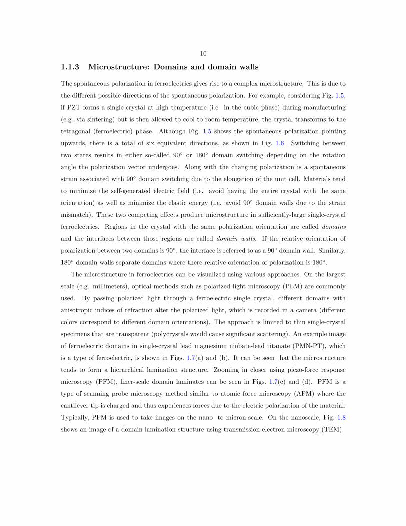
1.1.3 Microstructure: Domains and domain walls
The spontaneous polarization in ferroelectrics gives rise to a complex microstructure. This is due to
the different possible directions of the spontaneous polarization. For example, considering Fig. 1.5,
if PZT forms a single-crystal at high temperature (i.e. in the cubic phase) during manufacturing
(e.g. via sintering) but is then allowed to cool to room temperature, the crystal transforms to the
tetragonal (ferroelectric) phase. Although Fig. 1.5 shows the spontaneous polarization pointing
upwards, there is a total of six equivalent directions, as shown in Fig. 1.6. Switching between
two states results in either so-called 90 or 180 domain switching depending on the rotation
angle the polarization vector undergoes. Along with the changing polarization is a spontaneous
strain associated with 90 domain switching due to the elongation of the unit cell. Materials tend
to minimize the self-generated electric field (i.e. avoid having the entire crystal with the same
orientation) as well as minimize the elastic energy (i.e. avoid 90 domain walls due to the strain
mismatch). These two competing effects produce microstructure in sufficiently-large single-crystal
ferroelectrics. Regions in the crystal with the same polarization orientation are called domains
and the interfaces between those regions are called domain walls. If the relative orientation of
polarization between two domains is 90, the interface is referred to as a 90 domain wall. Similarly,
180 domain walls separate domains where there relative orientation of polarization is 180.
The microstructure in ferroelectrics can be visualized using various approaches. On the largest
scale (e.g. millimeters), optical methods such as polarized light microscopy (PLM) are commonly
used. By passing polarized light through a ferroelectric single crystal, different domains with
anisotropic indices of refraction alter the polarized light, which is recorded in a camera (different
colors correspond to different domain orientations). The approach is limited to thin single-crystal
specimens that are transparent (polycrystals would cause significant scattering). An example image
of ferroelectric domains in single-crystal lead magnesium niobate-lead titanate (PMN-PT), which
is a type of ferroelectric, is shown in Figs. 1.7(a) and (b). It can be seen that the microstructure
tends to form a hierarchical lamination structure. Zooming in closer using piezo-force response
microscopy (PFM), finer-scale domain laminates can be seen in Figs. 1.7(c) and (d). PFM is a
type of scanning probe microscopy method similar to atomic force microscopy (AFM) where the
cantilever tip is charged and thus experiences forces due to the electric polarization of the material.
Typically, PFM is used to take images on the nano- to micron-scale. On the nanoscale, Fig. 1.8
shows an image of a domain lamination structure using transmission electron microscopy (TEM).
11
ps
ps
180ps ps
90 domain switching
Figure 1.6: There are six equivalent directions of the spontaneous polarization in PZT: the fourshown here as well as in and out of the page.
Manufacturing large single-crystal ferroelectrics is difficult and expensive. The largest sizes that
are typically available have side lengths on the order of millimeters. Therefore, most structural
applications of ferroelectrics utilize their polycrystalline form (i.e. ferroelectric ceramics). Ferro-
electric ceramics are commonly manufactured using powder compaction and sintering processes.
Thus, the original grain size of the powder governs the resulting grain size in the material. How-
ever, in addition to grains, the microstructure of ferroelectric ceramics still contains domains within
individual grains. This can be seen in Fig. 1.9. One can see the granular structure formed through
powder compaction and sintering in Fig. 1.9(a) using Scanning Electron Microscopy (SEM), while
zooming in closer using AFM, one can see the domain lamination structure within individual grains
in Fig. 1.9(b).
The microstructure is not necessarily constant. In particular, the domain structure can be al-
tered by applying an external electric field. Applying a large electric field can cause domain switch-
ing (where the spontaneous polarization aligns with the external electric field). When multiple
domains are present, domain switching usually occurs by increasing volume fractions of favorably-
oriented domains and by a corresponding decrease of unfavorable domains through domain wall
motion. In-situ observation using PLM has shown evolution of the domain structure upon appli-
where (·) ∈ C (hats) denote complex-valued amplitudes (which contain phase-information on the
stresses and strains) and ω ∈ R is the mechanical loading frequency. Substituting (1.5) into (1.4)
18
yields
σ(t) =
[−ω
∫ t
−∞E(t− t′) sinωt′dt′ + iω
∫ t
−∞E(t− t′) cosωt′dt′
]ε(t),
τ(t) =
[−ω
∫ t
−∞G(t− t′) sinωt′dt′ + iω
∫ t
−∞G(t− t′) cosωt′dt′
]γ(t),
(1.6)
where Euler’s formula, eiωt = cosωt + i sinωt has been used. By inspection of (1.6), one can see
that the terms in brackets are the apparent complex-valued Young and shear moduli E∗ and G∗,
respectively, i.e.
σ(t) = E∗ε(t), τ(t) = G∗γ(t). (1.7)
In general, a complex number can be fully described by its magnitude and argument (i.e. z = Reiθ).
Therefore, the measurements of the dynamic moduli, |E∗| and |G∗|, and phase angles, δE and δG
describe the complex Young and shear moduli, respectively. Mathematically, these quantities are,
|E∗| =√
[Re(E∗)]2 + [Im(E∗)]2 =|σ||ε|, tan δE =
Im(E∗)
Re(E∗)= tan(arg ε− arg σ),
|G∗| =√
[Re(G∗)]2 + [Im(G∗)]2 =|τ ||γ|, tan δG =
Im(G∗)
Re(G∗)= tan(arg γ − arg τ),
(1.8)
where tan δE and tan δG are the loss tangents corresponding to the Young and shear modulus,
respectively. Thus, in experiments we measure the ratio of the amplitude of stress to strain to
obtain the dynamic moduli and compute the tangent of the phase difference between stress and
strain to obtain the loss tangent. As an example, the dynamic Young modulus and loss tangent can
be measured via application of a time-varying sinusoidal uniaxial stress using Dynamic Mechanical
Analysis (DMA) as shown in Fig. 1.11. The resulting strain lags behind the applied stress due to
the viscoelasticity of the material. The phase angle between the stress and strain is δ, thus the loss
tangent is tan δ. The dynamic Young modulus is the ratio of the amplitude of the stress to the
strain: |E∗| = σ/ε. Plotting stress versus strain reveals a hysteresis loop. The area enclosed by the
loops is related to the energy damped (absorbed) by the material. The higher the loss tangent, the
greater the hysteresis and damping.
19
σ(t)
ε(t)
σ(t)
ε(t)
ε(t)
σε
δ
t1.5
0.10.05
tan δ = 0
σ
ε
Figure 1.11: An example experiment to measure the viscoelastic properties of a material (i.e. thedynamic Young modulus and loss tangent) using harmonic loading in a DMA setup (an image of aBose Electroforce is shown here).
1.3 Motivation
With the basic concepts of ferroelectricity and viscoelasticity reviewed, the motivation for study-
ing the dynamic response of ferroelectrics is presented. The study of ferroelectric ceramics as
energy absorbing materials (in particular for reducing vibrations in structures) has been ongoing
for the past several decades. To this point, such applications can be separated into two categories,
where the material is either passively or actively controlled in order to mitigate vibrations. Within
these two categories are more specific methods to absorb energy. A typical method for creating
passively-controlled energy absorbers is to short-circuit the ferroelectric material through a shunt
resistor (Bachmann et al., 2012; Cross and Fleeter, 2002; Guyomar et al., 2008; Hagood and von
Flotow, 1991); a strain-induced voltage on the surface of the ferroelectric specimen creates a cur-
rent that dissipates energy through the resistor via heating. Similarly, others have investigated
embedding ferroelectric inclusions in a conducting metal matrix, where current generated by a
strain-induced voltage in the inclusion is dissipated in the metal matrix via Joule heating (Asare
et al., 2012; Asare, 2004, 2007; Goff, 2003; Goff et al., 2004; Kampe et al., 2006; Poquette, 2005;
Poquette et al., 2011). This type of material is difficult to manufacture due to depolarization of
inclusions at high temperature. An alternative is to actively control the ferroelectric material via
controlling an applied voltage to cancel out vibrations (Arafa and Baz, 2000; Bailey and Hubbard,
1985; Duffy et al., 2013; Fanson and Caughey, 1990; Forward, 1979; Hanagud et al., 1992; Sharma
et al., 2013; Zheng et al., 2011) and other methods (Kumar and Singh, 2009; Li et al., 2008; Lin and
20
Table 1.1: Structural damping approaches and some of the typical loss tangents achieved.
passive loss tangent
high-damping material layers in plates and beams > 1(Capps and Beumel, 1990; Wetton, 1979)tuned mass damper (Taranath, 1988) –piezoelectric damping via shunt resistor (Bachmann et al., 2012) 0.001− 1.0piezoelectric-metal matrix composites (Asare et al., 2012) 0.01
active loss tangent
vibration canceling –piezoelectrics during temperature-induced phase changes (Cheng et al., 1996) < 0.02stress induced domain switching (Chaplya and Carman, 2002a) < 0.1
Ermanni, 2004; Liu et al., 2010; Ngo et al., 2004; Richard et al., 1999; Tremaine, 2012; Trindade
and Benjeddou, 2002). Additionally, the viscoelasticity of ferroelectrics has been studied but only
under small electric fields (Budimir et al., 2004; Burianova et al., 2008) (i.e. when there is no
microstructure evolution due to domain switching). As described in Section 1.2, a common metric
for evaluating the ability of a material to absorb vibrational energy is to measure its loss tangent,
tan δ. The higher the loss tangent, the more the material reduces vibrations. The problem with
the passive methods is that they produce relatively small loss tangents (typically tan δ < 0.01)
over most mechanical frequencies while only achieving significant damping near the resonance of
the system (typically tan δ = 1.0). Furthermore, active methods add complexity and are limited
by the strains and forces achievable by piezoelectricity, which makes their application in stiff, mas-
sive structures challenging. A summary of the mechanical damping reached by the aforementioned
methods as well as others is shown in Tab. 1.1.
In order to achieve significant damping increase over many different frequencies, which is de-
sirable in aircraft applications (Simpson and Schweiger, 1998), a different mechanism must be
used. In addition, aircraft and spacecraft structures and other structural applications often require
high-stiffness materials to rigidly support heavy loads. However, the combination of high stiffness
and high damping is usually not present in common engineering materials, as shown in Fig. 1.12.
Therefore, we seek to explore new damping mechanisms in materials, in particular, the kinetics of
microstructure evolution in ferroelectrics ceramics (which already have a high stiffness). Previous
methods have focused the piezoelectric effect (only small electric fields and small stresses/strains
were applied). Instead, utilizing the full ferroelectric response of materials (i.e. including domain
21
10−8
10−7
10−6
10−5
0.0010.01
0.11.0
10−4
loss tangent (–)
den
sity
(g/c
m3)
0.5
1.0
2.0
4.0
8.0
Young
’sm
odul
us(G
Pa)
0.001
0.01
0.1
1
10
100
1000
diamondsapphire
siliconquartz
ceramics
metals
polymers
brasssteel
CuZn
aluminum
FeV
basaltcarbon fiber
granite
glass
cementmortarbone
polystyrene
epoxy acetalPMMAPTFE
wood
polyethylene
Neoprene
Figure 1.12: Plot of Young’s modulus, loss tangent, and density of common engineering materials(including ceramics, metals, and polymers). Common engineering materials lack both a high Youngmodulus and high loss tangent (denoted by the shaded area). Values were obtained from (Callisterand Rethwisch, 2009; Lakes, 1998).
22
switching) is studied. In particular we examine the viscoelastic response and compare with other
methods for vibration control. This approach was first examined about a decade ago but little has
been studied since then. In particular, Chaplya and Carman (2001a,b, 2002a,b) examined the dis-
sipation in ferroelectrics due to stress-induced domain switching while Jimenez and Vicente (1998,
2000) investigated dissipation from electric field-induced domain switching.
Exploring the viscoelastic properties of electromechanically-coupled materials such as ferro-
electrics may lead to new avenues of creating materials with controllable viscoelasticity. In a similar
manner to metallic materials, for which damping is the macroscopic manifestation of the motion of
point defects (Snoek, 1941; Zener, 1948) or dislocations (Eshelby, 1949; Granato and Lucke, 2004),
of grain boundary activities (Ke, 1947), or of heterogeneous thermoelastic mechanisms (Bishop
and Kinra, 1995; Zener, 1937, 1938), additional damping can arise from domain wall motion in
materials such as ferromagnets (Burdett and Layng, 1968; Gilbert, 2004; Wuttig et al., 1998) and
ferroelectrics (Abrahams et al., 1968; Harrison and Redfern, 2002). The motion and interaction of
domain walls in ferroelectrics with defects (Kontsos and Landis, 2009; Schrade et al., 2007) pro-
duce Debye peaks of dielectric losses (Gentner et al., 1978; Xu et al., 2001; Zhou et al., 2001) as
well as increased mechanical damping (Arlt and Dederichs, 1980; Asare et al., 2012) and hysteresis
effects (Cao and Evans, 1993; Chen and Viehland, 2000; Schmidt, 1981). This effect becomes even
more pronounced when the material is subjected to an electric field above the coercive field (Merz,
1954; Miller and Savage, 1958, 1960; Tatara and Kohno, 2004; Yin and Cao, 2001). Thus, by care-
fully controlling an applied electric field, microstructure kinetics via domain wall motion and the
resulting time-dependent response of ferroelectrics can be controlled. Therefore, the goal of the
thesis research was to fully characterize the kinetics of domain switching in ferroelectrics (through
experiments and modeling) for creating high stiffness, high damping structural materials and for
new methods of actuation.
1.4 Outline
To better understand the influence of domain switching kinetics on the overall viscoelastic response
of ferroelectrics, experiments are performed to measure the evolution of their viscoelastic stiff-
ness and damping throughout the entire electric displacement hysteresis. In particular, the effect
of different (multiaxial) mechanical and electrical loading rates on the kinetics of microstructural
23
changes, due to domain switching, are investigated. Furthermore, the influence of domain switching
on the overall structural response of ferroelectric specimens (i.e. throughout the resonance spec-
trum) is determined, which is important for understanding their impact in structural applications.
A continuum-mechanics model is also developed to capture experimental measurements and predict
the behavior of new materials to optimize their viscoelastic response. With a better understand-
ing of the viscoelastic properties of ferroelectrics, proof-of-concept experiments are performed to
demonstrate potential applications of domain switching in set-and-hold actuators and for structural
damping.
The following chapters first focus on experimental methods. As will become evident in the
following chapter, the need for new experimental techniques motivated the development of Broad-
band Electromechanical Spectroscopy (BES), which will be presented in Chapter 2. Using this new
method, the viscoelasticity of PZT under different electromechanical loading rates is presented and
discussed in Chapter 3. With the aid of a newly-developed continuum model derived in Chap-
ter 4, insight is gained on the material behavior and guidelines are provided for material design. In
Chapter 5, domain switching kinetics are exploited in PZT-based actuators to demonstrate their
set-and-hold actuation and structural damping capabilities. Finally, the main results of the thesis
research are summarized in Chapter 6.
24
Chapter 2
Broadband ElectromechanicalSpectroscopy
The following sections follow from our previously published papers 1 (le Graverend et al., 2015;
Wojnar et al., 2014), however some additional details are provided. Understanding and ultimately
technologically exploiting the electro-thermo-mechanically-coupled time-dependent properties of
materials (e.g., of ferroelectric materials or of composites containing ferroelectric phases) requires
currently-unavailable measurement capabilities. Indeed, most available experimental methods for
characterizing viscoelastic materials are commonly performed by forced and free vibration test-
ing (Zhou et al., 2005b) and are applicable over rather restricted portions of the time and frequency
by time-harmonic bending, torsion, or tension/compression. DMA apparatuses are versatile and
experiments can be performed over wide ranges of ambient conditions; temperatures ranging from
-150 to 600C can be achieved in certain DMA setups (TA Instruments, 2015). However, the
frequency range of DMA depends significantly on the sample and on the test apparatus used.
For example, state-of-the-art DMA devices (Perkin Elmer, 2014) typically cover at most 0.001 to
600 Hz, and their use is also limited to a maximum specimen stiffness of less than 1 GPa, which
1The method and experimental setup was described in le Graverend, J.B., Wojnar, C., Kochmann, D., 2015.Broadband Electromechanical Spectroscopy: Characterizing the dynamic mechanical response of viscoelastic materi-als under temperature and electric field control in a vacuum environment. Journal of Materials Science 50, 3656–3685.URL: http://dx.doi.org/10.1007/s10853-015-8928-x, doi: 10.1007/s10853-015-8928-x. Additional experimen-tal results and analysis are from Wojnar, C.S., le Graverend, J.B., Kochmann, D.M., 2014. Broadband control of theviscoelasticity of ferroelectrics via domain switching. Applied Physics Letters 105, 162912. URL: http://scitation.aip.org/content/aip/journal/apl/105/16/10.1063/1.4899055, doi: http://dx.doi.org/10.1063/1.4899055.
excludes testing of ceramics and metals in general. Usually, the inertia of the grips in contact
with specimens in DMA limits the maximum driving frequency of the apparatus. Also, gripping or
otherwise contacting stiff, brittle materials such as ferroelectrics (and ceramics) without damaging
the specimen is difficult in practice, hence a contactless measurement approach is needed.
The Inverted Torsion Pendulum (ITP) is such a method that uses contactless techniques (Ke,
1947). However, the ITP is typically used for low-frequency experiments (10−5 to 10 Hz), which
may be too slow for observing the influence of microstructural processes in ferroelectrics such as
domain wall motion (Jimenez and Vicente, 2000; Miller and Savage, 1958). Like DMA, the ITP is
also versatile and experiments have been performed over wide ranges of temperatures from cryogenic
to elevated temperatures (-285C to 1500C) under vacuum (D’Anna and Benoit, 1990; Gadaud
et al., 1990; Gribb and Cooper, 1998; Woirgard et al., 1977). The ITP has mainly been used
for characterizing metals and ceramics with Young moduli ranging from 10s to 100s of GPa. Its
contactless approach of applying forces electromagnetically to specimens makes the ITP attractive
for testing ceramics.
Although primarily used for measuring elastic moduli (Migliori et al., 1993), Resonant Ultra-
sound Spectroscopy (RUS) can determine the frequency-dependent viscoelastic moduli by scanning
the specimen’s resonance spectrum in a double-transducer actuator-sensor setup (Lee et al., 2000).
The frequency range of RUS instruments is larger than DMA as it does not require a mechanical
driver but relies upon piezoelectric actuation. However, it is affected by the piezo-cells’ resonance
frequencies and practical limitations. For typical specimen sizes, (Lee et al., 2000) and (Zadler et al.,
2004) (for example) report RUS results from about 10 kHz to 10 MHz and from 5 kHz to 100 kHz,
respectively. RUS has been performed under various ambient conditions such as temperatures rang-
ing from -193 to 247C (Kuokkala and Schwarz, 1992) and elevated pressures (Zhang et al., 1998),
but not under vacuum, which is desirable for reducing spurious damping. In addition, the specific
specimen geometry required by RUS makes applying uniform electric fields via surface electrodes
difficult. Thus, electromechanical loading in RUS has not been attempted. A similar method called
the Piezoelectric Ultrasonic Composite Oscillator Technique (PUCOT) (Daniels and Finlayson,
2006) tracks the specimen’s resonance spectrum in a forced-vibration cantilever configuration.
In a similar fashion to DMA, Broadband Viscoelastic Spectroscopy (BVS) performs bending and
torsion but uses contactless techniques (Dong et al., 2008; Lakes and Quackenbusch, 1996; Lakes,
2004): moments are applied by electromagnetism and deformation is characterized by a laser-
26
Table 2.1: Comparison of the various viscoelastic characterization methods with BES. BES isthe only method that allows for a wide range of viscoelastic materials to be tested in a contactlessfashion and in a vacuum environment while simultaneously controlling the temperature and applyingelectric fields.
DMA 10-3 to 102 Hz up to 1 GPa -150 to 600C – – –RUS 104 to 107 Hz tan δ < 10-2 -193 to 247C – – –ITP 10-5 to 10 Hz 10 to 103 GPa -268 to 1400C – X XBVS 10-6 to 105 up to 104 GPa up to 160C – – XBES 10 to 104 Hz up to 104 GPa up to 400C X X X
detector setup. Thus, BVS offers higher sensitivity and finer resolution than DMA and is capable
of scanning many decades of frequency (Brodt et al., 1995) with considerably lower compliance and
less spurious damping. Moreover, the contactless testing prevents damaging of the specimens. BVS
data has been reported for the range of roughly 10−6 to 105 Hz, i.e. covering approximately 11
decades of time and frequency (Lee et al., 2000). Of course, the exact frequency range depends on
the test instrument, the electronic function generator, the laser detector used, and on the sample.
Temperatures of up to 160C have been reached in the BVS apparatus used in (Dong et al., 2011,
2008, 2010) using convection heating via air flow, which unfortunately can lead to spurious damping.
The capabilities of the aforementioned methods are summarized in Tab. 2.1. Despite all these
techniques, electric fields and mechanical loads over significant ranges of frequency have not been in-
dependently applied before, which is necessary for fully-characterizing the thermo-electromechanical
response of ferroelectrics. Thus, a different method and setup is needed.
A new technique called Broadband Electromechanical Spectroscopy (BES) has been developed,
which measures the dynamic stiffness and damping of materials in a contactless fashion over a wide
range of frequencies while simultaneously applying an electric field in a vacuum environment. The
contactless testing allows for the characterization of brittle ceramics, the application of electric fields
allows for the electromechanical response of ferroelectrics to be measured, the vacuum environment
reduces spurious damping, and the apparatus allows for the temperature to be controlled. Thus,
BES allows for the viscoelastic characterization of ferroelectrics and other electro-active materials,
which was not possible with existing methods. The specific experimental setup used in the BES
technique will be explained in detail. The capabilities of the specific BES apparatus presented
are also given in Tab. 2.1 to compare with existing methods where it can be seen that BES can
27
test a wide range of viscoelastic materials under combined temperature and electric field control
in a vacuum environment, while still having the capability to apply a wide range of mechanical
frequencies as in BVS. A wide frequency range is important for characterizing the kinetics of
domain switching as well as understanding its impact on structural resonance. We note that the
BES method is more general than the specific apparatus presented here. In Chapter 3, using BES,
the dynamic stiffness and damping in bending and torsion of a ferroelectric ceramic, viz. PZT, are
measured during electric field-induced domain switching. Moreover, experiments performed in air
and under vacuum are compared to quantify the influence of the surrounding air on the measured
dynamic stiffness and damping.
2.1 Materials and methods used in Broadband Electrome-
chanical Spectroscopy
To study a wide range of materials with thermo-electromechanically coupled properties from soft
polymers such as PVDF (with a typical Young modulus of 3 GPa (Tamura et al., 1974)) to stiff
ferroelectric ceramics (which are studied here and have Young moduli on the order of 100 GPa) and
composites containing ferroelectrics (whose dynamic moduli can be as high as 104 GPa (Jaglinski
et al., 2007)), the specimens are tested in bending and/or torsion, as opposed to uniaxial tests.
Specimens with cantilevered beam geometry are gripped on one end and a bending and/or torsional
moment is applied to their free end, as shown in a schematic of the apparatus in Fig. 2.1. The
cantilever beam setup is best suited for testing materials under time-varying temperatures and
electric fields as both of which may cause eigenstrain in the material. The minimal grip contact
with cantilever beams (compared to 3-point or 4-point bending setups) minimizes the amount of
internal stresses arising from eigenstrain, which may influence the material response. In a similar
manner to BVS (Lakes, 2004), bending and torsional moments are applied through Helmholtz
coils via a permanent magnet attached to the specimen’s free end. Specimen deflection/twist is
captured via a laser-detector set-up as shown in 2.2(a). Adding to the capabilities of BVS, an
electric field is applied using surface electrodes on the specimen and electric displacements are
measured via a Sawyer-Tower circuit connected to the grips (Sawyer and Tower, 1930; Sinha,
1965). Furthermore, the BES apparatus comprises a vacuum chamber as shown in Fig. 2.2(a) to
reduce the influence of spurious damping. The temperature inside the chamber can be controlled
28
vertical coils used for bending
horizontal coils used for torsion
permanent magnet
grip electrode
vacuum
mirror
specimen
electrodes
grips
position sensor
laser
lock-inamplifier
waveformgeneratorin ref.
waveformgenerator
high-voltageamplifier
scope
V (t) = V cosωtu(t) = u cos(ωt+ δ)
t t Hy
Hz
Hy
Hz
My
Mz
µ
ex, dx
u, tan δ
chamber
window
Figure 2.1: Schematic of the apparatus showing the specimen gripped in the center. Above thespecimen are the two pairs of Helmholtz coils used for bending and torsion tests as in BVS. The coilsare shown in their raised position allowing for the specimen to be positioned. Once the specimenis gripped in place, the coils are lowered over the specimen such that the magnet is located at theintersection of the two coil axes. The specimen and coils are placed inside a vacuum chamber witha window for the laser beam to enter and reflect back to the position sensor outside. In the top-leftcorner appears the lock-in amplifier set-up connected to the position sensor with the applied voltageto the coils used as the reference signal. The bottom-right corner shows the Sawyer-Tower circuitused.
via radiant heating (as opposed to convective heating used in previous BVS setups, which can
effect damping measurements). However, experiments have so far all been performed at room
temperature. Electromechanical characterization of PZT at different levels of temperature would
nonetheless be a potential future direction of research. The overall size of the setup was designed for
testing polycrystalline specimens on the millimeter scale, which is the size of ferroelectrics typically
used in structural applications. The remainder of this section explains measurement techniques as
well as data acquisition and post processing in more detail.
specimen gripwith glass isolation(for application of
an electric bias field)
a)
b)
c) d)
e)
Figure 2.2: Pictures of the apparatus showing (a) the chamber in the operating position and howthe laser enters the chamber, is reflected by the mirror, and is detected by the position sensor, (b)the chamber in the raised position, (c) the coils and their support structure, (d) the specimen andattached clamp holding the permanent magnet that applies the electromagnetic force generated bythe coils to the specimen’s free end, and a mirror used to reflect the incoming laser beam to measurespecimen bending/twist, and (e) the specimen grip for the application of an electrical bias.
30
2.1.1 Force control
Due to the potentially large elastic moduli of the specimens to be tested, the compliance of the
apparatus is reduced to a minimum by utilizing contactless techniques. To this end, the apparatus
contains two pairs of Helmholtz coils (shown in Fig. 2.2(b,c)) for generating the driving magnetic
fields that produce a torque on the specimen (via a neodymium-iron-boron permanent magnet with
a maximum pull of 12 N attached to the specimen’s free end). These pairs of coils are used to apply
bending (vertical coils) and/or torsional (horizontal coils) moments to the specimen, as shown in
Fig. 2.1.
The coils are constructed by winding 32 AWG magnet wire around cylinders made of Macor
(3 cm diameter, 8 mm long, 150 turns). The coils are approximately rigidly held in place by a
supporting structure as shown in Fig. 2.2(b,c). The coils apply a moment to the magnet attached
to the specimen using a clamp also manufactured from Macor. The clamp contains one slot on each
side for attaching the specimen and magnet (Fig. 2.2(d)). For accurate thermo-electromechanical
testing, the material used for the clamp and the core of the coils must be stable over a large range
of temperatures (up to 1000 C), electrically insulating so as to not short-circuit the specimen
electrodes used to apply electric fields, non-magnetic so as to not interfere with the attached magnet
and coils, and sufficiently stiff to effectively transfer the force from the magnet to the specimen and
to minimize the compliance of the coil supports. Ceramic materials fulfill these criteria and Macor
was chosen for the ease with which it can be machined.
Current is passed through the coils by applying a time-varying voltage V (t) using a waveform
generator to produce approximately uniform magnetic fields Hz and Hy between each pair of coils.
The magnetic moment µ of the permanent magnet is oriented in such a way that the magnetic field
from the vertical and horizontal coils applies a bending moment Mz, and a twisting moment My,
respectively, to the magnet as shown in Fig. 2.1. Bending and/or torsional moments up to 10-4 Nm
can be applied with the current setup up.
2.1.2 Measuring the deflection and twist of the specimen
The total deflection and/or twist of the specimen is also measured in a contactless way using a
laser-detector setup: an incoming laser beam reflects off a mirror attached to the clamp and then
returns to a position sensor as shown in Figs. 2.1 and 2.2(a). The laser source (5 mW 633 nm
31
helium-neon laser from Research Electro-Optics, Boulder, CO, USA) and detector (SpotOn Analog
Positioning from Duma Optronics Ltd., Nesher, Israel) are placed outside the vacuum chamber.
The laser detector has a resolution of 1 µm and a response time of 60 µs. Thus, specimen deflection
must be above the detection limit of the sensor and at frequencies well below 16 kHz. Testing at
higher frequencies can be accomplished by a detector with faster response time. The chamber has
a window made of Kodial (transmission factor above 92 % for the laser wavelength) to allow for
the laser beam to be transmitted inside. Thus, the laser spot on the detector moves due to the
thermo-electromechanical response of the specimen. In particular, bending and twisting cause the
laser spot to move along the vertical and the horizontal axes of the sensor, respectively.
While applying the maximum bending or torsional moment, the maximum and minimum of
the Young and shear moduli that can be measured with the current setup is shown in Fig. 2.3 for
different specimen geometries. Fig. 2.3(a) shows the range in Young modulus (shaded region) that
can be measured versus the specimen thickness for different specimen lengths (from Euler-Bernoulli
beam theory). The maximum Young modulus that can be measured corresponds to the smallest
resolvable deflection in the laser detector, 1 µm (while applying the maximum bending moment and
for the chosen distance between the specimen and detector, 0.4 m). The minimum Young modulus
corresponds to the maximum deflection of the specimen for the same applied bending moment
before the laser beam moves off the detector (4500 µm). Similarly, the maximum and minimum
shear moduli that can be measured are shown in Fig. 2.3(b) versus specimen thickness for different
lengths.
2.1.3 Electric field control
To generate an electric field within the specimen, a voltage is applied across its thickness via
surface electrodes deposited, for example, by sputtering. To avoid connecting wires directly to
the specimen’s electrodes, the grips that hold the specimen are covered with copper tape in order
to apply a voltage, as shown in Figs. 2.1 and 2.2(e). This prevents the wires from affecting the
mechanical response of the specimen and avoids mechanical degradation of the electrical connection
when performing experiments over an extended period of time, e.g. during fatigue tests. In order to
electrically isolate the grip from the apparatus, the portion of the grip in contact with the specimen
that is covered with copper tape is fabricated from glass as shown in Fig. 2.2(e).
Under a large applied electric field, the ferroelectric materials of interest undergo microstructural
32
1 2 3 4 5 6 7 8 9 1010-3
10-2
10-1
1
10
102
103
104
105
specimen thickness (mm)
You
ng’
sm
od
ulu
s(G
Pa)
29 mm58 mm
116 mm
1 2 3 4 5 6 7 8 9 10specimen thickness (mm)
10-4
10-3
10-2
1
10
102
103
shea
rm
od
ulu
s(G
Pa)
10-129 mm
58 mm116 mm
specimen length:
specimen length:
a)
b)
Figure 2.3: Ranges of specimen (a) Young modulus and (b) shear modulus that can be tested usingthe current BES setup (shaded region) versus specimen thickness. Several regions are shown fordifferent lengths of the specimen.
33
evolution due to domain switching (i.e. reorientation of polarization through domain wall motion),
which causes the non-linear behavior of the electric displacement (Cao and Evans, 1993; Chen and
Viehland, 2000; Schmidt, 1981; Zhou et al., 2001). Changes in the macroscopic (average) electric
displacement of the specimen are measured using a Sawyer-Tower circuit (Sawyer and Tower, 1930).
In the circuit used, it was determined that a 100 µF reference capacitor was suitable for measuring
the charge accumulation on the specimen. For the electric loading rates tested (i.e. to induce domain
switching in the ferroelectric specimens, 0.01 to 1 Hz, triangle-wave voltages with amplitudes up to
±2000 V were applied), the impedance of the measuring scope (1 MΩ) was sufficient to minimize
charge leakage from the reference capacitor during experiments. An approximate calculation of the
influence of the charge leakage on the measured electric displacement is shown in Appendix A. The
high-voltage signal is provided by a waveform generator and amplified by a high-voltage amplifier
(10/10B-HS from Trek, Lockport, NY, USA), which can apply 0 to ±10 kV DC and supply 0 to
±10 mA DC as shown in Fig. 2.4(a).
2.1.4 Vacuum chamber
The apparatus is enclosed by a massive chamber (see Fig. 2.2(a)) with a vacuum seal and wall-
internal water cooling to allow for safe operation at high temperatures. The chamber also limits
environmental noise such as mechanical and thermal oscillations caused by the surrounding air. In
addition, the entire apparatus is placed upon Pneumatic Vibration Isolators (S-2000 series from
Newport, Irvine, CA, USA) to reduce vibrations from the building. The overall size of the apparatus
is determined by the specimen size to be tested (1×3×38 mm3), which itself is chosen so as to have
a sufficiently high natural frequency (130 Hz in bending, and 1300 Hz in torsion). In this way, the
mechanical loading of the specimen can be chosen well below the specimen’s structural resonance
frequency.
The vacuum is achieved after two stages of pumping: a primary pump (rotary vane pump from
Pfeiffer Vacuum, Asslar, Germany) and a secondary pump (turbomolecular pump from Pfeiffer Vac-
uum, Asslar, Germany) as shown in Fig. 2.4(b-d). These pumps allow the apparatus to reach a final
pressure of 1.9×10⁻⁶ mbar measured by a pressure gauge (active Pirani/cold cathode transmitter).
Controlling the pressure is essential when applying large voltages across the specimen. Indeed,
Paschen’s law gives the breakdown voltage between two parallel electrodes in a gas as a function of
pressure and gap length (Hourdakis et al., 2006; Paschen, 1889). This is typically modeled using
34
BES in operation
side view (left) side view (right)
venting valve
turbomolecularpump
water cooling out(obscured)
pressure measurement5× 10-9 to 1× 10³ mbar
(Active, Pirani/ColdCathode Transmitter)
feed-through4 pins, 1 kVdc, 20 A
feed-through2 pins, 5 kVdc, 30 A
and thermocouple
primary vacuum pumpon ceiling rack
ceiling mountedpulley for raisingand lowering
vibration damper
air cooling systemhigh voltage amplifier
dual-channel waveformgenerator
oscilloscope
lock-in amplifier
vacuum display
vacuum chamber
a)
b)
c)d)
Figure 2.4: Additional pictures of the apparatus: (a) shows the electronics rack containing thevarious instruments used during an experiment, (b) shows the primary pump sitting above theapparatus on a ceiling rack that is connected to the chamber via a hose, (c) shows the chamberviewed from the left hand side, and (d) shows the chamber viewed from the right hand side.
35
the equation (see e.g. (Lieberman and Lichtenberg, 2005)),
VB =Apd
ln(p d) +B, (2.1)
where p is the atmospheric pressure, d is the separation distance of the electrodes, and A and B
are constants associated with the composition of the gas and the electrode material. This behavior
has been extensively studied and characterized due to its importance for electronic packaging. See
e.g. (Cobine, 1941) for more information on this phenomenon. Fig. 2.5 contains experimental data
showing that the evolution of the breakdown voltage in air is not linear and highly depends on the
product of the pressure and the separation distance of the electrodes (approximately 1 mm for the
specimens tested). For atmospheric pressure, the voltage required for breakdown between electrodes
separated by 1 mm is 3×10³ V, and at first this decreases as the pressure decreases. However,
the voltage required for breakdown starts to increase as the pressure continues to decrease below
7×10⁻³ bar. Thus, with decreasing pressure, the risk of electrical arcing increases (in particular at
low voltages), unless the pressure is below the critical value (in which higher voltages are required
for arcing). This behavior is due to two competing effects that determine the voltage required for
electronic breakdown. On the one hand, decreasing the pressure reduces the likelihood an electron
will be scattered by a gas molecule (and thus prevent a conduction path from forming). This
gives rise to the breakdown voltage decreasing as the pressure is initially reduced from atmospheric
pressure. However, on the other hand, reducing the pressure reduces the number of gas molecules
available for ionization, which decreases the likelihood of electric breakdown. This effect dominates
at low pressures, and eventually gives rise to an increase in breakdown voltage as the pressure
is decreased further. For our purposes, voltages of up to ±2 kV were used in the experiments.
Therefore, from Fig. 2.5, a minimum vacuum pressure of 2×10⁻³ bar must be reached to prevent
electrical arcing when using the vacuum chamber. In typical vacuum experiments, pressures of
10-4 mbar or less were used.
2.1.5 Temperature control
The vacuum chamber is also used to accurately control the temperature of the specimen. Temper-
atures of up to 400C are achieved by radiant heaters placed inside of the chamber, a temperature
controller, and a 2.6 kW power supply (0-50 V-DC/0-52 A-DC from Magna Power, Flemington,
36
10-4 10-3 10-2 10-1 1 10 102102
103
104
106
105
p · d (bar-mm)
bre
akd
own
vol
tage
(V)
Figure 2.5: Evolution of the breakdown voltage in air as a function of the pressure p times theseparation distance of the specimen electrodes d (Picot, 2000).
NJ, USA). The outer walls of the chamber can also be water cooled for safe operation at elevated
temperatures.
The radiant heaters can draw a large current and generate a corresponding magnetic field which
could give rise to undesired forces on the specimen magnet. Therefore, the chamber was designed
to be large enough (0.2 m diameter) to ensure sufficient distance between radiant heaters and the
specimen. As a simple check, Ampere’s law can be applied to a disk enclosing and with normal
vector along the axis of the heaters (treated as a single infinitely long wire) as shown in Fig. 2.6.
The radius of the disk extends from the chamber wall (where the heaters are) to the center of
the chamber where the specimen is gripped; thus its radius is d/2 where d is the diameter of the
chamber. Ampere’s law then gives the magnetic field at the center of the chamber, due to one of
the heaters as
Bheat =µ0I
πd, (2.2)
where I = P/V is the current through the heaters and µ0 is the permittivity of air. The maximum
power and voltage of the power supply are P = 2.6 kW and V = 50 Vdc, respectively. The
specimen is placed at the center of the chamber, which has a diameter of roughly d = 0.207 m.
By inserting these values into (2.2) we obtain Bheat/µ0 = 80 A/m. The magnetic field generated
by the Helmholtz coils (treated as ideal, infinitely long solenoids) is Bcoil = µ0ni. There are 150
turns of wire and the solenoid is 8 mm long, thus n = 150/0.008 m-1. Typically, 7.2 V are applied
37
feed-throughs for
feed-throughs for
magnetic field line due to
Bheat
I
resistive heaters
Helmholtz coils and
current through heaters
specimen
Helmholtz coils
heaters
Sawyer-Tower circuit
Figure 2.6: Drawing showing the approximate location of the two graphite resistive heaters onopposite sides of the inside wall of the vacuum chamber. Also shown are the approximate locationsof cables for powering the Helmholtz coils, specimen surface electrodes, and heaters. It is importantthat the heater cables use a separate feed-through in the chamber wall on the opposite side to thefeed-through for the coils and specimen electrodes to prevent electromagnetic interference due tothe large heater current I creating a magnetic field Bheat.
and the resistance of the coils is roughly 30 Ω, thus i = 7.2/30 V/Ω. Therefore, the magnetic field
at the position of the specimen as generated by the coils is Bcoil/µ0 = 4500 A/m. We see the
magnetic field at the specimen due to the Helmholtz coils is two orders of magnitude higher than
the magnetic field at the specimen due to the heating elements (i.e. Bcoil Bheat). Therefore,
this effect can indeed be neglected. Furthermore, feed-through cables in the chamber wall for the
Helmholtz coils and Sawyer-Tower circuit are placed on the opposite side of those for the radiant
heaters as shown in Fig. 2.6, thus reducing interference between electrical cables.
In summary, this method improves upon currently available BVS techniques by utilizing a
radiative heating approach instead of heating by convection (which uses airflow). This enhances the
measurement accuracy of the specimen’s dynamic stiffness and damping by reducing measurement
artifacts caused by the airflow, especially at high temperatures. The addition of the Sawyer-Tower
circuit also adds the capability (beyond current devices) to apply electric fields and measure the
electric displacement of the specimens – an important addition that can be used to fully characterize
the thermo-electromechanical response of ferroelectrics and other materials whose properties can
38
be tuned by electric fields. BES can also test materials over a much larger range of mechanical
loading frequencies than DMA; in the current configuration, frequencies ranging from 1 Hz to
4 kHz can be tested directly. In general, the main limitations on the maximum frequency are due
to the waveform generator (max. 1 MHz), the lock-in amplifier bandwidth (max. 100 kHz), the
laser detector (max. 16 kHz), and the impedance of the coils (max. 4 kHz). The latter can reduce
the applied moment and decrease the signal-to-noise ratio at high frequencies. However, by using
lower impedance coils or a laser detector with a faster response, higher-frequency experiments can
be performed with this method. The lower limit on the frequency is due to temperature variations
and low-frequency noise. The apparatus is placed on an air vibration isolation table, which reduces
high-frequency noise but is susceptible to low frequency oscillations. For the current setup the most
accurate measurements were obtained above 1 Hz. To perform low-frequency tests, the isolation
table should be deflated or the apparatus placed on a more rigid support. However, all experimental
results reported in this article were obtained from frequencies not less than 25 Hz, thus the influence
of low-frequency noise was not significant.
2.2 Characterizing the material’s response
The following section explains the details of using measurements obtained from the BES setup to
compute the material properties. In particular, the data is used to infer the viscoelastic properties
(i.e. dynamic Young and shear moduli and their associated loss tangents) as well as the ferroelectric
properties (i.e. the electric displacement and thereby the state of polarization in a ferroelectric
material).
2.2.1 Measuring viscoelastic properties
A voltage, V (t) = V cos(ω t) with frequency ω, is applied to the Helmholtz coils, which results in a
current, i(t) = i cos(ω t+ φ). In a typical experiment, V ranges from 2.0 to 7.2 Vpp (peak-to-peak
voltage). The position of the laser beam in the detector, u(t) = u cos(ω t+δ+φ), is input to a lock-in
amplifier (SR830 from Stanford Research Systems, Sunnyvale, CA, USA) using the applied voltage
on the coils V (t) as the reference signal as shown in Figs. 2.1 and 2.4(a). The lock-in amplifier gives
a high-accuracy measurement of the laser spot movement at the same frequency as the reference
signal, which has a total phase shift of δ + φ, where δ is due to the viscoelasticity of the specimen
39
and φ is the phase shift associated with the frequency response of the coils. Note that the vertical
or horizontal position of the laser is selected when performing bending or torsion tests, respectively.
Noise present in the signal at different frequencies is filtered out by the lock-in amplifier. The cutoff
frequency fcutoff for the low-pass filter applied to the output of the phase-sensitive detector in the
lock-in amplifier was selected to be 5.3 Hz, which was determined to be sufficiently low to reduce
noise in the measurements but sufficiently high so that the response of the lock-in is faster than any
changes in the material response. Nominally, the cutoff frequency corresponded to a time constant
τ setting of 30 ms on the lock-in amplifier, i.e. τ = 1/(2πfcutoff). See Appendix B for a more
detailed analysis of the noise filtered by the lock-in amplifier. However, for different frequencies of
the applied electric field, a different time constant was used (see discussion in Section 3.4.3).
For experiments performed away from structural resonance, the expression for static deflec-
tion/twist at the end of the bar still applies for the dynamic case and the correspondence principle
can be applied with the elastic moduli replaced by their viscoelastic (complex-valued) ones (Lakes,
1998). When the mechanical frequencies approach the structural resonance frequencies, inertia ef-
fects become important and the static solution and the corresponding viscoelastic form obtained by
the correspondence principle no longer apply. In this case the following formulation should instead
be interpreted as the structural (i.e. geometry-dependent) response of the specimen. We proceed
to utilize the static solutions for the Euler-Bernoulli beam and uniform torsion problems with the
understanding that the solutions only give the material properties when experiments are performed
away from resonance, otherwise they result in the structural response.
For small deformations, the deflection and total twist angles at the end of the specimen are
θz =MzL
EIz, θy =
MyL
GJy, (2.3)
respectively, where Mz is the bending moment, L is the length of the specimen, E is the static
Young modulus, Iz is the bending moment of inertia along the z-axis with Iz = bh3/12 (b is the
width and h is the thickness) for rectangular cross sections, My is the torsional moment, G is the
static shear modulus, and Jy is the torsional moment of inertia along the y-axis (for rectangular
cross sections Jy = bh(b2 + h2)/12). Note that warping of the specimen’s cross section during
torsion is neglected. For a magnet with magnetic moment µ perpendicular to the axes of the coils,
the total applied bending and torsional moments on the specimen are Mz = µHy and My = µHz,
40
position sensor
mirror rotation dueto bending moment
mirror rotation dueto torsional moment
l
zy
uzuy
zy
θz
Mz
My θy
Figure 2.7: Illustration of the laser spot movement on the detector with components uz and uy dueto applied bending and torsional moments Mz and My, respectively.
respectively, where Hy and Hz are the magnetic fields generated by the vertical and horizontal
coils, respectively, as shown in Fig. 2.1. In a typical experiment, moments ranging from 10-5 to
10-4 Nm are applied. Assuming an ideal coil, the magnetic fields at the position of the magnet are
Hy = αznziz and Hz = αynyiy, where ni is the number of turns per unit length, ii is the current,
and αi is a geometric factor for the deviation of the magnetic field from the idealized infinitely
long solenoid and a subscript i = z or i = y corresponds to the respective values for the vertical
and horizontal coils. Altogether, the total bending and torsional moments, respectively, can be
expressed as
Mz = µαznziz, My = µαynyiy. (2.4)
The deflection angle and twist θz and θy are related to the directional changes in position of
the laser beam, uz and uy, in the detector by tan θz = uz/l and tan θy = uy/l, respectively, where
l is the distance between the specimen and the detector as shown in Fig. 2.7. For small deflections
and twist angles, this is approximated by θi ≈ ui/l. Combining this expression with (2.3) and (2.4)
results in the specimen’s Young and shear moduli,
E =µαznzizl
uzIz≡ Cz
izuz, G =
µαynyiyl
uyJy≡ Cy
iyuy, (2.5)
41
respectively, where the constants Cz and Cy depend on parameters associated with the apparatus
and geometry of the specimen, which were held constant for the experiments. For the dynamic
case, we use the correspondence principle, so that (2.5) still applies but with the moduli replaced
by their complex-valued counterparts, and the currents and displacements by their time-harmonic
amplitudes, i.e.
E∗ = Czizuz, G∗ = Cy
iyuy. (2.6)
Recall that the above relation holds for experiments performed away from resonance, and near
resonance the moduli are the structural ones. For the experiments shown later, we choose to report
the relative dynamic Young and shear moduli,
|E||E0|
=u0z
uz,
|G||G0|
=u0y
uy, (2.7)
respectively, where superscript 0 refers to the case with no applied electric field, and uz and uy
are the corresponding amplitudes of the laser spot motion on the position sensor (measured by the
lock-in amplifier). The loss tangents of the complex Young and shear moduli follow from (2.6)
tan δE = tan
[arg
(izuz
)], tan δG = tan
[arg
(iyuy
)]. (2.8)
In previous BVS setups, (2.8) is used where the applied current is measured as the voltage drop
across a resistor in series with the coils (Lakes, 1998). As mentioned previously, in the BES setup
the applied voltage to the coils is used as the reference signal for the lock-in amplifier instead of
the current. In this way, a resistor in series with the coils is not needed, which allows for higher
current through the coils (increasing the signal to noise ratio) and simplifies the electronic circuit.
However, the phase shift φ introduced by the coils must be accounted for in post processing the
phase signal output by the lock-in amplifier. Thus, when using the coil voltage as the reference
signal, (2.8) becomes
tan δE = tan
[arg
(Vzuz
)− φz
], tan δG = tan
[arg
(Vyuy
)− φy
], (2.9)
where Vz and Vy are the amplitudes of the applied voltages to the vertical and horizontal coils,
respectively, and φz and φy are the respective phase shifts between the voltage and resulting current.
42
non-magnetic (aluminum) pole coiled wire
scopescope resistor
a)
b)
Helmholtz coils
Figure 2.8: (a) Picture of the magnetometer made by coiling magnet wire and attaching it to theend of a pole so that it can be inserted between the Helmholtz coils. The diameter of the coiledwire was approximately 12 mm. (b) Illustrates how the magnetometer is placed in the Helmholtzcoils and the current through it is measured via a resistor.
2.2.2 Frequency response of the Helmholtz coils
To determine the specimen’s loss tangent from the lock-in amplifier output using (2.9), the phase
shifts φz and φy introduced by the coils were measured a priori. This phase difference was measured
by inserting a small solenoid (used as a magnetometer) collinear with either the horizontal or vertical
coils, see Fig. 2.8. The induced current in the small solenoid, due to the coils, was measured via a
resistor in series with the small solenoid. The frequency of the cyclically changing voltage in the
coils is small compared to the speed of light, which means the phase of the measured current is the
same as the magnetic field. Thus, the tangent of the phase difference between the applied voltage
to the Helmholtz coils and the resulting current (in phase with the magnetic field) was measured for
different frequencies and is shown in Fig. 2.9(a) for the vertical (bending) and horizontal (torsion)
coils.
To quantify the frequency response of the coils, consider an electronic circuit consisting of a
voltage source with frequency ω, coils modeled as an inductor with inductance L, and a resistor R
to account for the wire resistance. This is an RL circuit where the tangent of the phase difference
43
frequency (Hz)0 500 1000 1500 2000 2500 30000.70
0.75
0.80
0.85
0.90
0.95
1.00
bendingcoils
torsion coils
0
0.1
0.2
0.3
0.4
0.5
0.6
frequency (Hz)0 200 400 600 800 1000 1200
bending coils
torsion coils
a) b)ta
nφ
ofco
ils
(–)
M/M
0(–
)
tanφ = 4.70e-4s×f
tanφ = 4.19e-4s×f
Figure 2.9: (a) Variation of the tangent of the phase between the applied voltage and magneticfield of the Helmholtz coils (tanφ) with the frequency of the applied voltage to the bending andtorsion coils. (b) The change in the amplitude of the applied moment M relative to the amplitudeat 0 Hz (M0) versus the frequency of the applied voltage to the bending and torsion coils.
between the voltage and current and the impedance are given by
tanφ = ω L/R, Z =√R2 + (ωL)2, (2.10)
respectively, where the current amplitude through the coils is then given by i = V /Z. The resistance
of the wires R for the bending and torsion coils was measured to be 25.8 Ω and 22.4 Ω, respectively.
The inductance L can then be found from equating tanφ in (2.10) to the slopes of the trend lines
in Fig. 2.9(a). It was found that the inductances of the vertical and horizontal coils were 1.4
and 0.8 mH, respectively. Using the inductance obtained, φ can be computed for the frequency
being used in the experiment. The measured inductances of the coils can also be compared to
the theoretical result obtained by using the standard formula for a cylindrical air-core solenoid,
L = µ0K n2A/l, where µ0 = 4π × 10−7 H/m is the permeability of free space, the Nagaoka
coefficient K (Nagaoka, 1909) is a correcting factor for the non-ideal geometry of the coils (typically
1 for slender solenoids), n is the number of turns, A is the cross-sectional area of each coil, and l is
the length of each coil. For the coils used, this gives K = 0.8821 and K = 0.9183 for the vertical
and horizontal coils, respectively. For the maximum frequency used in experiments (3 to 4 kHz)
the phase difference of the coils can be as high as tanφ = 1.57. Thus, it is important to correct for
this phase shift when using the coil voltage as the reference for the lock-in amplifier.
From (2.10), the impedance of the coils is also frequency dependent. The increase in the
44
impedance of the coils with increasing frequency causes the amplitude of the applied moment on
the specimen to decrease with increasing frequency (for a constant amplitude voltage on the coils).
As shown in (2.4), the applied moment is related to the current in the coils via M = µαn i. Using
the frequency-dependent impedance of the coils, this becomes, M = µαnV /Z(ω), which is plotted
in Fig. 2.9(b) after normalizing by M0, the moment at 0 Hz. For the frequencies used, the applied
moment decreases by up to 30 %. However, the applied moments are small such that the response
of the material is in the linear viscoelastic regime. Thus, the variation of the applied moment does
not effect the viscoelastic properties measured, a result which will be confirmed in Section 3.4.4.
Although results presented here were all from tests performed at room temperature, one must
carefully correct for the phase shift due to the coil impedance when varying the temperature.
Therefore, the coil impedance should be pre-determined for the temperature(s) of interest. For
varying temperature, a more elegant and more accurate approach is to use the current in the coils
as the reference for the lock-in as described in (Lakes, 1998) for BVS.
2.2.3 Approximate methods for extracting the material properties near
resonance
The above methods yield the structural response of the specimen from measurements taken during
an experiment. To find the material response, it is best to perform the experiment away from
resonance so that inertial effects are small and the static solution for the beam deflection/twist and
the viscoelastic form obtained by the correspondence principle apply. For the specimens tested,
this applied for frequencies below 130 Hz in bending and 1300 Hz in torsion. When mechanical
loading frequencies approach the resonance frequency, a different geometry specimen can be used
with a different resonance frequency. As an alternative, an approximate correction can be applied
to the structural measurements near resonance to obtain the material properties.
The bending problem can be approximated by a spring-mass-dashpot system subjected to an
external force F as shown in Fig. 2.10, where the linear spring stiffness k and velocity proportional
damping c represent the apparent stiffness and damping of the cantilever beam. The total mass
of the attached magnet, mirror, and clamp corresponds to m. Force balance of the spring-mass-
dashpot system in terms of the deflection w yields
k w + c w +mw = F. (2.11)
45
m
w(L, t)
w(L, t)m
k c
F F
Figure 2.10: A cantilevered beam with tip deflection w(L, t) due to an applied force F and withattached mass m is approximated by a spring-mass-dashpot system with stiffness k, mass m, anddamping c.
Assuming a harmonic solution w = w eiωt due to a time-varying force F = F eiωt, the complex
modulus is
k∗ = F /w = k −mω2 + iωc. (2.12)
Thus, taking the absolute value and tangent of the argument of (2.12) yields the structural dynamic
stiffness and loss tangent as
|k∗| = k
√√√√[1−(ω
ω0
)2]2
+(ω ck
)2
, tan δk =ω c/k
1− (ω/ω0)2, (2.13)
where ω0 =√k/m is the resonance frequency. The structural loss tangent (tan δk) becomes the ma-
terial loss tangent (tan δ) when the frequency is well below the resonance frequency (i.e. ω/ω0 1)
and inertial effects are small, which yields tan δ = ωc/k. Using this result, equations (2.13) can be
solved for the material properties k and tan δ in terms of the structural properties |k∗| and tan δk,
which gives
k =|k∗|
[1− (ω/ω0)2]√
1 + (tan δk)2, tan δ = tan δk
[1− (ω/ω0)2
]. (2.14)
Finally, the spring stiffness follows from the linear elastic beam solution (i.e. k ∝ E), and normal-
ization as in (2.7) yields:
E0(ω → 0)
E(ω)=|E0|(ω → 0)
|E|(ω)
√1 + [tan δE(ω)]2
1 + [tan δE(ω → 0)]2[1− (ω/ω0)2
], (2.15)
where |E0|(ω → 0) and tan δE(ω → 0) are taken at 25 Hz where inertial effects are small (i.e.
ω/ω0 1). The ratio |E0|(ω → 0)/|E|(ω) is computed from (2.7). The material loss tangent is
46
then simply
tan δEmat = tan δE[1− (ω/ω0)2
]. (2.16)
The same result for the torsion case can be derived where the problem is approximated by a torsional
spring with damping and a mass with rotational inertia. Then, from linear elasticity, k is replaced
by the torsional stiffness of the beam and normalized to obtain
G0(ω → 0)
G(ω)=|G0|(ω → 0)
|G|(ω)
√1 + [tan δG(ω)]2
1 + [tan δG(ω → 0)]2[1− (ω/ω0)2
],
tan δGmat = tan δG[1− (ω/ω0)2
].
(2.17)
In a similar manner to the bending case, |G0|(ω → 0) and tan δG(ω → 0) are taken to be at 25 Hz
where inertial effects are small, and |G0|(ω → 0)/|G|(ω) is obtained from (2.7).
The accuracy of this approach can be seen by applying the corrections to the solution of a
dynamic cantilevered Euler-Bernoulli beam (using expressions derived in Appendix C) with known
constant compliance and loss tangent. The correction derived in equations (2.15) and (2.16) are
applied to the predicted structural dynamic response of the Euler-Bernoulli beam given by (C.6).
Both the structural and approximated material responses are shown together in Fig. 2.11. In
addition, Fig. 2.11 shows the constant material (static) compliance and loss tangent. For both the
compliance and loss tangent, Fig. 2.11 shows that while the structural response increases greatly
near the first resonance, the approximate material response remains close to the constant static
value. (Although the approximation increasingly deviates from the correct material response as the
first resonance frequency is approached and surpassed.) Nonetheless, the approximated response
still yields values for the compliance and loss tangent that are closer to the true material response
up to the first resonance frequency. In should be noted that, in practice, pure bending or torsion is
not achieved, due to small misalignments (as discussed in Section 3.4.2). Thus, when applying the
corrections in bending or torsion, the approximation may not hold at particular frequencies due to
resonance modes that are not accounted for by our analysis, which only considers the case of pure
bending and pure torsion.
Another possible way to find the material response is to assume that the response of the specimen
47
10 102 10310-2
10-1
1
10
frequency (Hz)rela
tive
com
pli
ance
inb
end
ing
(–)
10 102 103
frequency (Hz)
10-2
10-1
1
ben
din
glo
ssta
nge
nt
(–)
static value dynamic value corrected value
a) b)
Figure 2.11: Comparison of the theoretical dynamic (a) compliance and (b) loss tangent (longdashed line) with their corrected response (solid line) using (2.15) and (2.16), respectively, for anEuler-Bernoulli beam. The parameters used are given in Tab. 3.2. The material compliance andloss tangent were taken to be constant and are shown by the short dashed line.
is the same as an Euler-Bernoulli beam with complex moduli, i.e. substituting
E → E(1 + i tan δEmat), G→ G(1 + i tan δGmat) (2.18)
into the solutions derived in Appendix C for the dynamic Euler-Bernoulli beam and torsion problem.
Thus, the dynamic Young modulus and loss tangent become
|E∗| =
∣∣∣∣∣Mz
θz
∣∣∣∣∣ , tan δE =Im(Mz/θz
)Re(Mz/θz
) . (2.19)
Equating the left-hand-sides of (2.19) with the experimental measurements results in two equations
for the two unknown material properties E and tan δEmat. Similarly for the torsion case, the
dynamic shear modulus and loss tangent become,
|G∗| =
∣∣∣∣∣My
θy
∣∣∣∣∣ , tan δG =Im(My/θy
)Re(My/θy
) . (2.20)
Comparing (2.20) with experimental measurements also yields two equations for the two unknown
material properties G and tan δGmat. However the assumption that the material behaves like an
Euler-Bernoulli beam may not be accurate, especially near higher resonances where the approxima-
48
tion of the clamp as a point mass is not exact. One could also, in principle, perform a finite element
analysis, which better captures the geometry of the specimen, to find the appropriate material pa-
rameters that best reproduce the experimental measurements. In addition, resonance methods as
described by Lakes (1998) can be used to obtain a material’s loss tangent at resonance. However,
such an approach is complicated by the fact that (as observed in the experiments of Chapter 3) the
resonance frequency of the material changes due to the application of an electric field, which makes
it difficult to define a resonance peak in the structural loss tangent.
2.2.4 Measuring electric displacement and electric field
The electrical response of the material is characterized by the specimen’s macroscopic (average)
electric displacement as shown in Fig. 2.12. The electric displacement is measured by a Sawyer-
Tower circuit, as shown in Fig. 2.1. Changes in the electric displacement in the material (due
to domain switching and electric field-dipole interaction) cause a charge Q to accumulate on the
specimen’s surface electrodes. The same charge Q accumulates on the reference capacitor and
is reflected in its voltage Vcap = Q/C (here an electrolytic capacitor was used with capacitance
C = 100 µF). The macroscopic electric displacement through the specimen thickness dx is then
given by the total charge on the specimen divided by the surface area of the electrodes, i.e.
dx =C Vcap
b L. (2.21)
When applying cyclic electric fields, dielectric loss of the capacitor can lead to hysteresis in the
electric displacement. However, for characterizing the electromechanical response of ferroelectrics,
such capacitors are commonly used at frequencies of 1 Hz or less (Zhou et al., 2001) (which is the
case here as well) and thus their dielectric loss is not significant (Zhou, 2003).
The high-voltage amplifier applies a known voltage Velec to the surface electrodes of the specimen.
The applied electric field ex through the specimen thickness h is
ex =Velec
h. (2.22)
The aspect ratio of the specimen’s surface area to thickness is assumed to be sufficiently large so
that variations in the electric field near the edges are negligible. Moreover, the capacitance of the
49
p(x) p
Figure 2.12: Illustration of how a polycrystalline specimen in a Sawyer-Tower circuit has spatially-varying polarization p(x) which gives rise to an average polarization p that is reflected in the chargemeasured on the surface electrodes.
specimen is significantly smaller than the reference capacitor so that the voltage applied to the
specimen is nearly the same as that applied by the high-voltage amplifier (i.e. the voltage drop
across the reference capacitor is negligible). For a typical experiment, the high-voltage amplifier
applied 2 kV while the voltage on the reference capacitor is 1 V. Therefore, the presence of the
capacitor reduces the actual applied voltage to the specimen by 0.05 %.
2.3 Sources of error
Before performing experiments, various possible sources of error in the experimental setup were
analyzed to ensure that their influence on the measurements were negligible (at least under the
nominal conditions). In particular, the effects of laser misalignment, parasitic damping due to
support loss, and electromagnetic coupling are explained and analyzed in the following sections.
2.3.1 Resolution of the laser detector
Due to the resolution of the sensor in the laser detector, there is an uncertainty in the position of the
laser spot of 1 µm. As the position of the laser spot is used in determining the specimen’s Young
and shear moduli, the resolution of the detector causes some uncertainty in their measurement.
This uncertainty was quantified by measuring the deflection of a PZT specimen while applying
the maximum static bending moment, 10−4 Nm. For a specimen with the same geometries tested
(given in Tab. 3.2), the Young modulus was computed assuming an Euler-Bernoulli beam (i.e.,
using (2.3)) based on the laser beam position in the detector, which was 70 µm relative to its
undeformed position. The Young modulus from the Euler-Bernoulli beam changed by 1 GPa upon
50
modifying the laser position by 1 µm, the sensor resolution. Therefore, the uncertainty in the
Young modulus measured for the PZT specimens is ±1 GPa. The Young modulus (in the loading
direction) reported by the supplier in Tab. 3.1 is 66 GPa. Thus, the uncertainty in the Young
modulus is less than 2%. Using the same approach, the uncertainty for the shear modulus was also
less than 2%.
2.3.2 Effect of laser misalignment
The strain due to polarization changes (which gives rise to the well-known butterfly curve as shown
in e.g. (Zhou et al., 2001)) causes specimens to bend/twist one way or the other during a cycle of the
electric field. That is, the laser spot on the detector oscillates about a mean value (due to the applied
dynamic mechanical load), but this mean value changes slowly during the experiment due to the
spontaneous strain in the material in response to the applied electric bias, whose frequency is much
lower than the mechanical loading frequency. For the ferroelectrics tested, the spontaneous strain
was never sufficient to cause the laser spot to leave the linear range of the detector. Nonetheless, it
is important to verify that the slowly-changing mean position of the laser spot does not considerably
affect the measurement of the dynamic moduli, which is related to the inverse of the amplitude of
the laser spot movement via (2.7). For an illustration of this phenomenon, see Fig. 2.13 where it
can be seen that changes in the laser position change the apparent amplitude of the laser motion.
The problem will be analyzed in the case of bending. However, the same conclusions apply to the
case of torsion. Under an applied mechanical loading, the deflection of the end of the specimen
subtends an angle 2θ. The laser beam travels a distance l to the detector. Then, assume that the
average specimen deflection changes (due to some eigenstrain) such that the laser now travels at an
angle φ causing an average displacement ∆ on the sensor. From the geometry, the two amplitudes
can be written as
u0y = 2 l tan θ, uy = l [tan(φ+ θ)− tan(φ− θ)] . (2.23)
Using trigonometric identities and making the substitution tanφ = ∆/l, the ratio of the two
amplitudes can be written as
u0y
uy=
1− (∆/l)2 tan2 θ
1 + (∆/l)2≈ 1− (1 + tan2 θ)(∆/l)2. (2.24)
51
specimen mirror position sensor2θ
2θ φ
u0y
uy
∆
l
Figure 2.13: Illustration of the effect of the average laser position on the amplitude of the signal(not to scale).
For the stiff materials of interest, θ is small. Therefore, as long as ∆/l is small, the effects of
eigenstrains in the material during testing can be considered small. For example, as a worst-case
approximation, let ∆ be the size of the detector (1 cm), let θ = φ, and take l to be 0.29 m (the
actual distance in the apparatus), then u0y/uy = 0.999, which is much smaller than the changes in
the moduli measured (i.e. as much as 0.6 measured in the bending experiments of Section 3.2).
The measured phase lag will be unaffected by the misalignment of the laser since the mechanical
bending frequencies tested are many orders of magnitude slower than the speed of light of the laser
beam, which would have to travel slightly farther due to misalignment.
2.3.3 Parasitic damping due to support loss
The specimen grip and surrounding vacuum chamber are designed to be stiff and massive to mini-
mize the effect of the apparatus compliance on the specimen. However, the propagation of elastic
waves into the grip and support structure can increase the measured damping of the specimen. This
phenomenon has been analyzed in (Hao et al., 2003), where they compute the traction imparted by
a vibrating cantilever (assumed to be of the same material as the grip for simplicity) attached to
an elastic half-space as shown in Fig. 2.14. From the analysis in (Hao et al., 2003), the following
closed-form expression was found for the apparent quality factor Q of a perfectly elastic specimen
52
grip
specimen M(t)t
Figure 2.14: Illustration of a cantilevered beam specimen attached to a grip modeled as an elastichalf-space. Harmonic bending of the specimen generates elastic waves that travel away through thegrip and cause energy loss (or damping).
due to the energy loss through elastic waves,
Q =0.24(1− ν)L3
ψ(1 + ν)(βnχn)2h3,
ψ =
∫ ∞0
√ξ2 − (cL/cT )2
[2ξ2 − (cL/cT )2]2 − 4ξ2
√ξ2 − (cL/cT )2
√ξ2 − 1
dξ,
(2.25)
where ν is the Poisson ratio of the elastic support material, L is the length of the specimen,
h is the specimen’s thickness, and cL and cT are the longitudinal and shear wave speed of the
support, respectively. The βn and χn are shape factors for a particular resonance mode, e.g. for
the first mode, they are 0.597 and -0.734, respectively (Hao et al., 2003). For a material such
as steel Poisson’s ratio is 0.28 and ψ = 0.336. Using the closed-form result for the estimation of
the measured quality factor of the specimen Q = (tan δ)−1, the loss tangent due to loss through
the support structure is estimated to be 1.8 × 10⁻⁵ at the first resonance frequency (using the
dimensions of the specimen in Tab. 3.2). The loss tangents measured in experiments were on the
order 0.01 to 1.0 as shown later in Section 3.2; thus, the influence of support loss on the measured
loss tangent is negligible.
2.3.4 Electromagnetic coupling
Although the ferroelectric materials of interest such as PZT are not magnetostrictive (i.e. stresses
do not generate magnetic fields and vice versa), the application of large, time-varying electric fields
53
to the specimen while simultaneously applying time-varying magnetic fields via Helmholtz coils can
lead to interference between the two fields. In addition, the metallic screws used to attach the
magnet and clamp to the specimen may experience small forces due to applied magnetic fields. To
measure the incremental stiffness and damping of materials under electric fields, it is necessary to
use mechanical frequencies that are much higher than the electric field frequencies. As a result, it
is expected that there is little interference between the two. Furthermore, the dielectric response
of PZT causes electric charges to accumulate on surface electrodes, which partially shield the
surrounding space outside of the specimen from the electric field generated by the applied voltage,
which further reduces the electromagnetic coupling. Indeed, this coupling between electric and
magnetic fields was found to be negligible in experiments. Experiments in bending and torsion were
repeated after removing the attached magnet. The specimen deflection amplitudes were compared
between tests with and without the permanent magnet (at 25 Hz, well below the first resonance
frequency of the two specimens). In this case the amplitude of the signal from the laser position
sensor (due to the specimen deflection) was measured to be at least 50 mV, with the attached
magnet, for the bending experiments. Upon removing the magnet, the signal amplitude was near
the resolution of the detector, 5 mV. Therefore, the effect of electromagnetic coupling in bending
is small and can be neglected. A similar result was observed for the case of torsion. Near anti-
resonance frequencies, when the deflection amplitude is near the detection limit, electromagnetic
coupling may be important (along with noise in the system). Altogether, electromagnetic coupling
in the setup does not affect the measured results. However, this effect may become important when
testing comparable electric and magnetic field frequencies.
2.3.5 Noise measurements
To obtain an overall picture of the noise in the apparatus, the total noise floor was characterized by
computing the power spectral density of the specimen deflection (in bending) under forced vibration
at 75 Hz as shown in Fig. 2.15. The power spectral density was computed using the MATLAB
function pwelch() on the laser position sensor output voltage. The amplitude of the signal at the
driving frequency is much higher by at least four decades than noise occurring at other frequencies
due to e.g. main voltage sources at 60 Hz and higher harmonics. As mentioned before, the current
setup is susceptible to noise at low frequencies (i.e. below 1 Hz) as evident in Fig. 2.15 where the
power spectral density increases significantly. However, such low frequencies were not currently of
54
10-2 10-1 1 10 103 104-120
-100
-80
-60
-40
-20
0
frequency (Hz)
pow
ersp
ectr
ald
ensi
ty(d
B/H
z)
102
Figure 2.15: Power spectral density of the laser position sensor output when applying a mechanicalbending frequency of 75 Hz and 7.2 Vpp amplitude. The signal power at 75 Hz, due to the appliedmoment, is much higher than noise occurring at other frequencies.
interest and thus experiments were not performed at those frequencies. To reduce noise at lower
frequencies, the apparatus should be placed on a more rigid table or the isolation table should be
deflated. However, by doing so, higher-frequency noise will be increased.
2.4 Validation
To demonstrate the accuracy of BES, experiments were performed to characterize already well-
known behaviors of materials and compare them with results in the literature. The viscoelas-
tic characterization capability of BES is shown through experiments performed on polymethyl
methacrylate (PMMA), whose stiffness and damping have been well characterized (Koppelmann,
1958), as well as aluminum. Second, the Sawyer-Tower circuit is used to characterize the evolution
of the electric displacement of PZT, which has also been extensively studied in the literature (Zhou
et al., 2001). In addition, comparison of the electric displacement evolution in air and under vacuum
is discussed.
55
frequency (Hz)1 10 102 103 104
10-2
10-1
1
10
frequency (Hz)1 10 102 103 104
10
1
0.1
0.01
100
ben
din
glo
ssta
nge
nt
(–)
rela
tive
ben
din
gco
mp
lian
ce(–
)experiment theory
Figure 2.16: Viscoelastic response of a PMMA sample measured using BES with (a) showingthe relative compliance and (b) showing the loss tangent in bending versus frequency. Blue pointsrepresent experimental data and solid black lines correspond to the dynamic Euler-Bernoulli solutionusing the parameters in Tab. 2.2.
2.4.1 Viscoelastic characterization of PMMA
A specimen of PMMA was cut to a size of 63.10 × 5.44 × 2.50 mm3 and its dynamic compliance
(inverse of Young’s modulus) and loss tangent in bending were measured for frequencies from 25-
2540 Hz as shown in Fig. 2.16. The compliance shows the typical resonance and anti-resonance
behavior. That is, there is a large increase in the compliance (i.e. increase in the deflection
amplitude) at a frequency of approximately 80 Hz, corresponding to the first resonance frequency.
Then the compliance decreases significantly at 113 Hz, corresponding to the first anti-resonance
frequency where the amplitude of the deflection becomes very small. This behavior is repeated for
higher-frequency resonance modes. The behavior of the loss tangent also shows the typical large
increase at resonance and anti-resonance frequencies. Note that to obtain positive loss tangents
(physically admissible), the absolute value of the output of the lock-in amplifier phase angle is used.
To determine Young’s modulus and loss tangent from the experiments, the solution of the
dynamic Euler-Bernoulli beam in (C.6) is fit to the experimental data as shown in Fig. 2.16 by
selecting the appropriate static Young modulus and loss tangent, which are assumed to be frequency
independent (that is, by substituting E → E(1+ i tan δEmat) and comparing |E∗| and tan δE to the
experimental data). The parameters used in the Euler-Bernoulli beam model are shown in Tab. 2.2.
The value of the static Young modulus and loss tangent that best match the experimental data
56
Table 2.2: Measured and fitted parameters of the PMMA specimen.
parameter symbol value
Young’s modulus* E 3 GPabending loss tangent* tan δE 0.05density ρ 1180 kg/m3
clamp mass m 1.412 gspecimen free length L 54.92 mmspecimen width b 5.44 mmspecimen thickness h 2.50 mm
* values obtained by fitting to experimental data
were 3 GPa and 0.05, respectively, which agree well with literature values. Young’s modulus is
reported to vary between 2.24 and 3.24 GPa (Callister and Rethwisch, 2009) and a loss tangent
of 0.1 at 1.0 Hz is reported in (Koppelmann, 1958). The discrepancy in the loss tangent is likely
due to variations between specimens due to e.g. material processing and preparation. Therefore,
the BES apparatus developed minimizes sources of error and results in accurate measurements of
dynamic stiffness and damping.
2.4.2 Loss tangent of aluminum
To get an idea of the smallest loss tangents that can be resolved and measured with the current BES
setup, the loss tangent of a low-loss (aluminum) specimen was measured. The specimen dimensions
were 63.5×6.5×1.1 mm3 cut from a sheet of aluminum 6061. A loss tangent of 0.005 was measured
at a subresonance frequency of 10 Hz. A loss tangent of 0.001 was reported for aluminum in (Zener,
1948). Variations in material processing and cutting likely cause variations in the loss tangent
between specimens that account for this discrepancy. Nonetheless, BES was able to resolve loss
tangents on the order of 10−3, which is well below the loss tangents that will be reported for PZT
in Chapter 3, viz. near 0.1. Thus, in the worst case, the error in the loss tangent measured for PZT
is no greater than 1%.
2.4.3 Electric displacement evolution in PZT
A triangle-wave electric field was applied to PZT specimens and the resulting macroscopic electric
displacement was measured using the Sawyer-Tower circuit setup in BES. The electric displace-
57
ment was measured for different frequencies of applied bending/twisting moments as well as for
different frequencies of the applied electric field. First, Fig. 2.17 shows the electric displacement
versus electric field for different electric field frequencies ranging from 0.01 to 1.0 Hz while applying
a bending moment at 75 Hz, which reveals the typical hysteresis curves obtained in numerous pre-
vious (static) studies, see e.g. (Hooker, 1998; Viehland and Chen, 2000; Zhou and Kamlah, 2006;
Zhou et al., 2001). Similarly, Fig. 2.18 shows the electric displacement versus electric field for the
same frequencies but while applying a torsional moment at 75 Hz. The important result is that the
coercive field increases with electric field frequency, which is consistent with (Zhou et al., 2005a)
for PZT and (Yin and Cao, 2002) for PZN-PT. There is asymmetry in the hysteresis curves with
respect to the electric field. Such behavior has been observed for initially-poled PZT (the specimens
tested here were also initially poled), see e.g. (Arlt and Neumann, 1988; Carl and Hardtl, 1977) for
a discussion of this phenomenon. The asymmetry is due to an internal bias in the material formed
during manufacturing when specimens are initially poled. The asymmetry has been shown to vanish
after a large number of electric field cycles (Carl and Hardtl, 1977). The value of the coercive field
(where the electric displacement crosses zero) in each direction is important for determining when
domain switching occurs in order to explain the results obtained for the dynamic moduli and loss
tangents shown in later experiments. In particular, domain switching occurs around the coercive
field where there is highly non-linear behavior of the electric displacement corresponding to polar-
ization reorientation in the material. Comparing the results obtained during bending and torsion
in Figs. 2.17 and 2.18, respectively, shows slightly different coercive fields as well as spontaneous
polarization (the value of the electric displacement at zero electric field). This difference is likely
due to variation in the electrical properties of the two specimens tested.
For a fixed electric field frequency of 0.1 Hz, Fig. 2.19(a) shows the electric displacement versus
electric field for various bending frequencies, which reveals similar hysteresis behavior as observed
in Figs. 2.17 and 2.18. However, the individual curves for different mechanical bending frequencies
coincide; the mechanical loading frequencies tested had no effect on the electric displacement hys-
teresis. That is, the stresses reached during mechanical loading had no influence on the evolution of
the average polarization in the material. There is also asymmetry in the hysteresis curves. Specifi-
cally, the spontaneous polarization and coercive field for a positive electric field are 1.49 MV/m and
0.37 C/m2, respectively, while for a negative electric field, they are - 1.36 MV/m and - 0.33 C/m2,
respectively. Similarly, Fig. 2.20(a) shows the electric displacement hysteresis for different torsional
58
-2.0 -1.0 0.0 1.0 2.0
-0.4
-0.2
0.0
0.2
0.4
electric field (MV/m)
elec
tric
dis
pla
cem
ent
(C/m
2)
0.01 Hz
0.1 Hz
0.5 Hz
1.0 Hz
electric cycling frequency:
Figure 2.17: Variation of the electric displacement versus electric field for different triangle-waveelectric field frequencies ranging from 0.01 to 1.0 Hz while applying a bending moment at 75 Hz.
-2.0 -1.0 0.0 1.0 2.0
-0.4
-0.2
0.0
0.2
0.4
electric field (MV/m)
elec
tric
dis
pla
cem
ent
(C/m
2)
0.01 Hz
0.1 Hz
0.5 Hz
1.0 Hz
electric cycling frequency:
Figure 2.18: Variation of the electric displacement versus electric field for different triangle-waveelectric field frequencies ranging from 0.01 to 1.0 Hz while applying a torsional moment at 75 Hz.
59
-2.0 -1.5 -1.0 -0.5 0 1.5 2.01.00.5
-0.4
-0.2
0
0.2
0.4
electric field (MV/m)
elec
tric
dis
pla
cem
ent
(C/m
2)
-2.0 -1.5 -1.0 -0.5 0 1.5 2.01.00.5
-0.4
-0.2
0
0.2
0.4
electric field (MV/m)
elec
tric
dis
pla
cem
ent
(C/m
2)25 Hz 100 Hz 400 Hz 1000 Hz vacuum air
a) b)
Figure 2.19: Electric displacement versus an applied cyclic electric field at 0.1 Hz: (a) effect of differ-ent mechanical bending frequencies (25-1000 Hz), (b) comparison between experiments performedin air and vacuum at a fixed mechanical frequency of 100 Hz.
-2.0 -1.5 -1.0 -0.5 0 1.5 2.01.00.5
-0.4
-0.2
0
0.2
0.4
electric field (MV/m)
elec
tric
dis
pla
cem
ent
(C/m
2)
-2.0 -1.5 -1.0 -0.5 0 1.5 2.01.00.5
-0.4
-0.2
0
0.2
0.4
electric field (MV/m)
elec
tric
dis
pla
cem
ent
(C/m
2)25 Hz 100 Hz 400 Hz 1000 Hz vacuum air
a) b)
Figure 2.20: Electric displacement versus an applied cyclic electric field at 0.1 Hz: (a) effect ofdifferent torsion frequencies (25-1000 Hz), (b) comparison between experiments performed in airand under vacuum at a fixed mechanical frequency of 100 Hz.
frequencies. Again the curves coincide with each other (as was the case with the hysteresis curves
obtained during bending). Thus, not only do the mechanical loading frequencies not affect the evo-
lution of the macroscopic polarization, bending and torsional moments also do not have an impact
on the evolution of the macroscopic polarization.
Comparing the electric displacement hysteresis in air and vacuum as shown in Figs. 2.19(b)
and 2.20(b) for a mechanical bending or torsion frequency of 100 Hz reveals a slight decrease in the
coercive field when performing cyclic electrical loading in vacuum compared to air. This effect may
be due to the hydrostatic pressure applied by the surrounding air; hydrostatic pressure has been
observed to affect the electric displacement hysteresis (Valadez et al., 2013).
60
2.5 Summarizing the capabilities of BES
The BES method and apparatus have been explained in detail in the previous sections. The
relevant capabilities (i.e. bandwidth and amplitude/resolution) of the specific equipment used
in the current BES setup are summarized in Tab. 2.3 along with explanations of some of their
limitations. In particular, the equipment used in the setup for applying mechanical loads and
measuring deformation, applying electric fields and measuring polarization, controlling temperature,
and generating a vacuum are distinguished. The maximum range in mechanical loading frequencies
that can be tested (due to the combined limitations of each piece of equipment) was reported
previously in Tab. 2.1 for BES. Thus, Tab. 2.1 shows that a wide range of mechanical loading
frequencies can be tested with the current apparatus (although slightly smaller than BVS) while
controlling temperature and applying electric fields (necessary for characterizing the viscoelastic
properties of ferroelectrics), which none of the other methods are capable of. It should also be
stressed that the capabilities presented in Tab. 2.3 correspond to the specific equipment of the
apparatus that was fabricated for testing ferroelectric ceramics. However, different equipment may
be used to tailor the capabilities of the setup for testing other materials under different conditions.
61
Table 2.3: Amplitude of thermo-electromechanical loading and pressure that can be supplied by andthe resolution of the material response that can by detected by the equipment used in the currentBES apparatus and their associated bandwidths. Notes are provided that describe the particularlimiting factor on the amplitude and/or bandwidth of some of the equipment.
equipment bandwidth amplitude/ notesresolution
mechanical loadingwaveform generator 10-3 to 106 Hz up to ±10 VHelmholtz coils and magnet up to 104 Hz up to 10-4 Nm limited by coil impedancelock-in amplifier 10 to 105 Hz 10-9 to 1 V noise at low frequencies
from tablelaser detector up to 104 Hz 1 to ±4500 µm
electrical loadingwaveform generator 10-3 to 106 Hz up to ±10 Vhigh-voltage amplifier up to 105 Hz up to ±103 VSawyer-Tower circuit 10-2 to 102 Hz up to 100 µC frequency-dependent
capacitance of electrolyticcapacitor
oscilloscope up to 106 Hz 10-3 to ±20 V
temperaturepower supply (4 kW) quasistatic up to 25 Adc
at 160 Vdcgraphite resistors quasistatic r.t. to 400C
vacuum chambervacuum pump quasistatic 10-9 to 1 bar vacuum depends on
quality of o-rings
62
Chapter 3
Experiments on PolycrystallineLead Zirconate Titanate
Using BES, the dynamic Young and shear moduli as well as the loss tangent in bending and torsion
of a ferroelectric ceramic were measured while simultaneously applying a large, slowly-varying cyclic
electric field at room temperature. With the present apparatus, dynamic tests are performed at
previously unattainable mechanical and electric cycling frequencies. Furthermore, each test was
performed in air at atmospheric pressure and under vacuum to demonstrate the improvement in
accuracy of measurements by removing the effects of air. Some of the following experiments and
discussions follow from our previous papers 1 (le Graverend et al., 2015; Wojnar et al., 2014).
It should be noted that generally, the specimens tested are orthotropic and thus for our purposes,
the Young modulus corresponds to the transverse one, Eyy, and the shear modulus corresponds to
the out-of-plane one, Gxy, as shown in Fig. 3.1 (or, using typical naming conventions for transversely
isotropic piezoactuators, E1 and G13, respectively, as used by the manufacturer). Only when the
macroscopic polarization is zero (due to random orientations of the polarization within each grain),
does the material display an approximately isotropic response. Thus, the Young modulus and shear
modulus measured in the following sections follow from our naming convention.
1The experiments performed at different mechanical frequencies were shown and discussed in le Graverend,J.B., Wojnar, C., Kochmann, D., 2015. Broadband Electromechanical Spectroscopy: Characterizing the dynamicmechanical response of viscoelastic materials under temperature and electric field control in a vacuum environ-ment. Journal of Materials Science 50, 3656–3685. URL: http://dx.doi.org/10.1007/s10853-015-8928-x, doi:10.1007/s10853-015-8928-x. The effect of electrical loading frequency was presented for the bending case in Woj-nar, C.S., le Graverend, J.B., Kochmann, D.M., 2014. Broadband control of the viscoelasticity of ferroelectrics viadomain switching. Applied Physics Letters 105, 162912. URL: http://scitation.aip.org/content/aip/journal/apl/105/16/10.1063/1.4899055, doi: http://dx.doi.org/10.1063/1.4899055.
Figure 3.1: Drawing of the components of the imposed stresses and strains during bending andshearing, which are used to define the Young and shear moduli for the generally orthotropic material.
3.1 Materials
All measurements were performed using initially-poled Navy-type II lead zirconate titanate (PZT,
PSI-5A4E from Piezo Systems Inc., Woburn, MA, USA), which is polycrystalline. This material is
widely used in commercial applications, and thus is of interest in this study. The relevant material
properties are listed in Tab. 3.1. The specimens were cut to 1× 3× 38 mm3. The largest (top and
bottom) surfaces of the specimens were coated with 10 µm thick nickel electrodes by the supplier.
Typical grain sizes in the specimens were 2 µm, as observed by Scanning Electron Microscopy (see
Fig. 3.2).
3.2 Bending experiments
By activating the vertical coils in BES, bending moments are applied to the specimens and the
resulting deflection angle is measured. Using the analysis in Section 2.2.1, the dynamic Young
modulus and loss tangent are obtained. Various frequencies of the applied bending moment and of
the applied electric field were tested to characterize the effect of mechanical and electrical loading
rates.
64
Table 3.1: Physical properties of the PSI-5A4E soft PZT ceramic at room temperature (obtainedfrom Piezo Systems Inc., Woburn, MA, USA).
material property symbol value
relative dielectric constant εr 1800Curie temperature Tc 350Clongitudinal strain-electric field coupling coefficient d33 390× 10−12 m/Vtransverse strain-electric field coupling coefficient d31 −190× 10−12 m/Vlongitudinal electric field-stress coupling coefficient g33 24× 10−3 Vm/Ntransverse electric field-stress coupling coefficient g31 −11.6× 10⁻³ Vm/Nlongitudinal electromechanical coupling coefficient k33 0.72transverse electromechanical coupling coefficient k31 0.35longitudinal Young modulus E3 66 GPatransverse Young modulus E1 52 GPamechanical quality factor Q = (tan δ)−1 80
30 µm
Figure 3.2: An image of a typical PZT specimen obtained from Scanning Electron Microscopy.Image is taken of the side of the specimen without the electrode (there was no surface preparationbefore imaging). Horizontal striations are due to the blade used by the manufacturer to cut speci-mens to size. Examining the surface reveals a granular structure with grains on the order of 2 µm.The image was obtained under 20 kV with a working distance of 10.6 mm. The magnification is2500×.
Figure 3.3: Relative Young modulus measured in air and under vacuum while applying a cyclicelectric field at 0.1 Hz. Results for several mechanical frequencies are shown: (a) 25 Hz, (b) 100 Hz,(c) 400 Hz, and (d) 1000 Hz. The Young modulus during electrical cycling is normalized by theYoung modulus when no electric field is applied, as presented in equation (2.7).
3.2.1 Different mechanical frequencies
Specimens were tested in bending to obtain the relative dynamic Young modulus and loss tangent
for various mechanical loading frequencies. The relative dynamic Young modulus (normalized by
the value at zero electric field) and the loss tangent are shown in Figs. 3.3 and 3.4, respectively, at
bending frequencies of 25, 100, 400, and 1000 Hz. At each mechanical loading frequency a sinusoidal
voltage was applied to the coils, with peak-to-peak amplitude V = 7.2 V. The electric field cycling
frequency was held constant at a 0.1 Hz triangle waveform with a 1.95 MV/m amplitude. Recall
that the mechanical loading frequency did not affect the evolution of the macroscopic electric
displacement, cf. Fig. 2.19(a).
Fig. 3.3 shows the relative dynamic Young modulus for different mechanical loading frequencies
in air and under vacuum. For each mechanical frequency the modulus displays softening near
Figure 3.4: Loss tangent in bending measured in air and under vacuum while applying a cyclicelectric field at 0.1 Hz. Several mechanical frequencies have been examined: (a) 25 Hz, (b) 100 Hz,(c) 400 Hz, and (d) 1000 Hz.
the coercive field. Away from the coercive field, the modulus varies linearly, which is due to the
change of the elastic constants with applied electric field (Fu and Zhang, 2000a; Wang et al., 2003a)
in addition to changing volume fractions of differently-polarized domains with anisotropic elastic
constants (Burlage, 1965; Yin and Cao, 2001, 2002). Comparing the results obtained in air and
under vacuum, there are only marginal effects on the measured modulus. However, consistent with
observations made of the electric displacement (slightly higher coercive fields in air), the minimum
Young modulus appears at slightly higher electric fields when experiments are performed in air
compared to under vacuum, which is when domain switching occurs.
The effect of the mechanical loading frequency on the loss tangent is shown in Fig. 3.4. For each
case, the loss tangent increases substantially near the coercive field, indicating additional dissipation
caused by domain wall motion. Linear variations away from domain switching can be attributed
to the electric field dependence of the complex elastic constants, which has been measured before
in (Wang et al., 2003b). For the case of 25 Hz in Fig. 3.4(a), the loss tangent is 0.11 at zero
Figure 3.5: Transient behavior of the relative Young modulus at 25 Hz (a) versus time (along withthe electric field) and (b) versus electric field (arrows indicate increasing time). Upon switching offthe electric field, the relative dynamic Young modulus decays to a different steady-state value thanthat observed at zero electric field during electric field cycling.
electric field and becomes as large as 0.28 near the coercive field – an increase by more than 250%.
It is important to point out that the loss tangent at 0 MV/m shown here is noticeably higher
than typical values reported in the literature (e.g., 0.01 to 0.015 in (Jimenez and Vicente, 2000),
and 0.0125 reported by the supplier). This is attributed to domain wall motion as follows. Even
though the electric field passes through 0 MV/m, this does not imply that all domain walls are
in equilibrium. The plots shown in Figs. 3.3 and 3.4 are obtained after at least one cycle of the
electric field where the measured response reaches a steady behavior. However, upon switching
off the electric field permanently, as shown in Figs. 3.5(a) and 3.6(a), there is a transient time
of about 1 s during which the stiffness and loss tangent change before reaching their steady-state
equilibrium values. This can also be seen in the corresponding plots of relative Young modulus and
loss tangent vs. electric field in Figs. 3.5(b) and 3.6(b), respectively, where the modulus increases
and the damping decreases at zero electric field. In this final steady state, the relative modulus
increases by 5% and the loss tangent in bending reaches approximately 0.02, which is close to the
reported literature values. A similar behavior was observed in (Jimenez and Vicente, 2000), where
a completely different DMA-type setup was used. Therefore, this behavior is not an artifact of the
experimental setup. The phenomenon is observed across different mechanical loading frequencies.
This behavior is also observed in torsion experiments and when testing different electric cycling
frequencies, and will be discussed in Sections 3.3 and 3.2.2, respectively.
The effect of air on the measured loss tangent – in particular on the maximum damping reached –
Figure 3.6: Transient behavior of the loss tangent in bending at 25 Hz (a) versus time (along withthe electric field) and (b) versus electric field (arrows indicate increasing time). Upon switchingoff the electric field, the loss tangent decays to a different steady-state value than that observed atzero electric field during cyclic electric fields.
is more significant than the impact on the Young modulus. This is most pronounced near resonance,
when the bending amplitude is highest (as observed in (Anderson et al., 1996)), which can be
attributed to the generation of acoustic waves in the surrounding air and will be examined more
closely in Section 3.4.2. Moreover, the damping peaks for the vacuum appear for lower electric field
values for all mechanical frequencies studied here, which is again consistent with the small changes
in the coercive field between air and vacuum.
Additional mechanical frequencies beyond those shown in Figs. 3.3 and 3.4 were also tested, up
to 5 kHz. For conciseness and to more easily see their trends with mechanical bending frequency,
the variations of the compliance (inverse of Young’s modulus) and the loss tangent with mechanical
frequency are shown in Fig. 3.7 with the compliance normalized by the static value (taken at 25 Hz)
and zero electric field. Experimental data points illustrate the compliance at zero electric field
(ex = 0) and the maximum compliance occurring near the coercive field (ex = ec). The compliance
shows the structural response, increasing up to the first resonance frequency at approximately
120 Hz and then decreasing significantly up to the first anti-resonance frequency at approximately
250 Hz. The behavior is repeated for the second resonance and anti-resonance frequencies occurring
at approximately 1200 Hz and 3000 Hz, respectively. The curve of the compliance near the coercive
field exhibits the same behavior but is shifted to lower frequencies. This is due to the softening in
the modulus seen in Fig. 3.3, near the coercive field, which causes a decrease in each (anti-)resonance
frequency. The loss tangent in Fig. 3.7(b) also shows the structural response, viz. increased damping
near resonance and anti-resonance frequencies. In addition, the damping measurements at the
69
coercive field are higher than at zero electric field due to the increase in domain wall motion near
the coercive field.
For frequencies below resonance, both the measured dynamic Young modulus and the loss
tangent showed small variations with mechanical frequency, in particular their respective minimum
and maximum values achieved during domain switching, as shown by the red curve in Fig. 3.7
(or in Fig. 4.3). Damping increases slightly with frequency and at high mechanical frequencies it
is ultimately assisted by the structural resonance of the specimen (occurring at 147 Hz under no
electric field and decreasing during switching due to reduction in the elastic modulus (Wang et al.,
2003b)). Previous experiments showed a damping decrease with increasing frequency (Jimenez
and Vicente, 2000); however, those experiments were performed at elevated temperatures, which
is expected to decrease the relaxation time associated with domain switching (Savage and Miller,
1960). Experiments at ultrasonic frequencies (10 MHz) also revealed significant damping in single
crystals (Yin and Cao, 2001); yet, those primarily exploited the elastic anisotropy, to be controlled
by electric fields that affect the volume fractions of differently-polarized domains. Here, the kinetics
of the domain switching process itself produces remarkable variations in stiffness and damping.
Fig. 3.7 compares the solution of the dynamic Euler-Bernoulli beam with an attached end mass
(representing the clamp), as derived in Appendix C, to the experimental results. The two curves
were obtained by using the material’s static Young modulus and 65% of the static Young modulus
(which corresponds to the softened value near the coercive field). Also, the loss tangents were
selected to be 0.09 and 0.28 (three times higher) for the two cases (assumed to be constant with
frequency). The Young modulus was also assumed to be frequency independent and was fit to the
experimental results, which resulted in the specimen parameters of Tab. 3.2. The fitted Young
modulus was less than the modulus reported by the supplier in Tab. 3.1. This discrepancy may be
due to variation of material properties between particular specimens as well as approximations of
the Euler-Beroulli model and clamp. A more sophisticated model will be developed in Chapter 4.
Nonetheless, one can see that the Euler-Bernoulli solution agrees well with the behavior around
the first (anti-)resonance frequency, but starts to deviate at higher frequencies likely due to the
approximation of the clamp as a point mass. In particular, by decreasing Young’s modulus in
the Euler-Bernoulli solution, the resonance behavior shifts to lower frequencies, as observed in the
experiments.
Near resonance frequencies, the experimental results presented correspond to the structural
70
10 102 103 10410-3
10-2
10-1
1
10
102
frequency (Hz)
rela
tive
ben
din
gco
mp
lian
ce(–
)
10 102 103 104
frequency (Hz)
10-3
10-2
10-1
1
10
ben
din
glo
ssta
nge
nt
(–)
experiment: theory:ex = 0 ex = ec ex = 0 ex = ec
a) b)
Figure 3.7: The compliance (a) and the loss tangent (b) in bending are shown vs. mechanicalfrequency for two different values of the applied electric field (red and blue points) and are comparedto the theoretical Euler-Bernoulli solution (red and blue dashed lines).
Table 3.2: Measured and fitted parameters of the specimen.
parameter symbol value
Young’s modulus* E 35 GPashear modulus* G 10 GPabending loss tangent* tan δE 0.09torsion loss tangent* tan δG 0.1density ρ 6776 kg/m3
clamp mass m 1.594 gclamp moment of inertia Im 2.14× 10⁻⁸ kg m4
specimen free length L 30.46 mmspecimen width b 3.62 mmspecimen thickness h 1.04 mmapplied moment M 6× 10⁻⁵ Nm
* values obtained by fitting to experimental data
71
10 102 10310-1
1
10
102
frequency (Hz)
rela
tive
ben
din
gco
mp
lian
ce(–
)
102 103
frequency (Hz)
10-2
10-1
1
ben
din
glo
ssta
nge
nt
(–)
corrected:experiment: ex = ecex = 0
10a) b)
ex = 0 ex = ec
10
Figure 3.8: Summary of the results from Fig. 3.7 after applying the corrections in (2.15) and (2.16)to obtain the material response up to the first resonance frequency.
Young modulus and loss tangent. To obtain the material properties near resonance, the corrections
derived in (2.15) and (2.16) were applied to the results in Fig. 3.7 to obtain the approximate
material response shown in Fig. 3.8. In particular, the first resonance frequencies, ω0, for the
bending case used in (2.15) were 123 and 101 Hz for the measurements at zero electric field and
at the coercive field, respectively. There are much smaller variations in the material compliance
and loss tangent compared to the structural one (i.e. they do not increase sharply close to the
first resonance frequency). Thus, the approximate method for finding the material response gives
a more accurate value than when using the structural response.
3.2.2 Effect of electrical loading frequency
Fig. 3.9 illustrates the variations of stiffness and damping for electric field cycling frequencies of
0.01, 0.1, 0.5, and 1 Hz at a constant mechanical bending frequency of 75 Hz and amplitude of
7.2 Vpp. Recall that the corresponding electric displacement measurements were already shown in
Fig. 2.17, which in particular shows how the coercive field increases with electric field frequency.
After the onset of domain switching (near the coercive field when the polarization is changing the
most), the dynamic Young modulus softens significantly, to below 70% of its original value without
electric fields, see Fig. 3.9(b). The faster the electric field cycling, the greater the softening effect.
As observed in single-crystalline PZN-PT (Yin and Cao, 2001), the modulus variation is partly
due to elastic anisotropy: 90-switched domains, observed in polycrystals under cyclic electric
72
fields (Tsurumi et al., 1997), reduce the apparent modulus in the loading direction. This effect
is more gradual in polycrystals (Burlage, 1965) due to the distributed grain orientations. Linear
variation of the modulus with electric field before and after switching was also observed in PZT
polycrystals in (Wang et al., 2003b).
The loss tangent shown in Fig. 3.9(c) exhibits peaks during domain switching, which become
more pronounced with increasing electric field frequency. Like the dynamic Young modulus, the
loss tangent varies linearly with the electric field before and after domain switching (as observed
previously (Wang et al., 2003b)). The remarkable damping seen during domain switching with
tan δ > 0.4 is commonly found in polymers, rarely in ceramics. Its physical origin is similar to that
found in single crystals (Yin and Cao, 2001) but the polycrystalline orientation distribution leads
to a more gradual evolution of the macroscopic viscoelastic properties.
The rate-dependent stiffness and damping variations have been attributed to 90-domain switch-
ing (Arlt and Dederichs, 1980; Chaplya and Carman, 2002a). For higher electric field frequencies,
the domain wall velocity increases (Merz, 1956; Miller, 1958; Miller and Savage, 1958, 1959a,b, 1960,
1961; Tatara and Kohno, 2004), which leads to an accelerated repoling process, see Fig. 3.9(a). This
in turn results in larger spontaneous longitudinal strains during each mechanical cycle, thereby de-
creasing the apparent modulus. Also, the increases in domain wall velocity and apparent coercive
field (which increases the domain-wall driving force) together increase the dissipated energy. Owing
to the analogous thermodynamic driving force (or energy momentum tensor) arising from surfaces of
discontinuities (Abeyaratne and Knowles, 1990; Eshelby, 1975), similar phenomena can be expected
from domain wall motion in ferromagnetic materials (James, 2002; Wuttig et al., 1998).
3.3 Torsion experiments
The previous tests in bending generally gave rise to states of uniaxial stress and strain for small
amplitudes, which allowed for the apparent Young modulus to be measured. BES also has the
capability to apply torsional moments in order to measure the specimen’s response in shear and
characterize the apparent shear modulus. Here, similar experiments to those in bending are per-
formed where the torsional frequency and electric field frequency are varied independently.
Figure 3.9: Experimental data of (a) relative Young modulus (normalized by the modulus with-out electric bias) and (b) loss tangent in bending vs. electric field for triangle-wave electric field(1.8 MV/m amplitude) frequencies of 0.01, 0.1, 0.5, and 1.0 Hz, and constant bending vibration at75 Hz.
3.3.1 Different mechanical frequencies
Specimens were characterized in torsion with the same experimental conditions as in bending. The
effect of torsional mechanical frequencies of 25, 100, 400, and 1000 Hz on the relative dynamic
shear modulus (normalized by the value at zero electric field) and loss tangent were measured in
air and under vacuum as shown in Figs. 3.10 and 3.11, respectively. The torsional moment was
generated by applying a sinusoidal voltage, with peak-to-peak amplitude V = 6.0 V, to the coils.
Recall that the different torsional frequencies did not affect the evolution of the macroscopic electric
displacement as shown in Fig. 2.20.
The qualitative nature of the curves for the normalized dynamic shear modulus (Fig. 3.10) are
similar to those observed in bending; the modulus changes linearly away from the coercive field
(due to the change of the elastic constants with electric field and anisotropy of changing volume
fractions of differently-polarized domains) but exhibits less softening at the coercive field during
domain switching than in bending for all the mechanical frequencies tested. For example, at 25 Hz
during bending, Young’s modulus decreases to approximately 60% of its value at zero electric field,
while the shear modulus only decreases to approximately 70% of its value at zero electric field (and
it should be noted that experiments for determining the effect of mechanical loading frequencies in
bending and torsion were all performed using the same PZT specimen). This seems to indicate that
domain reorientation has more of an effect on the Young modulus than the shear modulus. This is
Figure 3.10: Relative shear modulus measured in air and under vacuum in torsion while applyinga cyclic electric field at 0.1 Hz. Several mechanical frequencies are shown: (a) 25 Hz, (b) 100 Hz,(c) 400 Hz, and (d) 1000 Hz. The shear modulus during electrical cycling is normalized by theshear modulus when no electric field is applied, as presented in (2.7).
theorized to stem from the effect of changing volume fractions of anisotropic phases on the Young
modulus is larger than on the shear modulus (which involves volume-preserving deformations). The
loss tangent in torsion for different mechanical frequencies is shown in Fig. 3.11. As in bending,
there is a large increase in damping near the coercive field due to domain switching (an increase
by nearly a factor of three) and a linear variation away from the coercive field due to the electric
field dependence and anisotropy of the complex elastic constants. As was the case in bending,
the measured loss tangent at 0 MV/m is noticeably higher than typical values of PZT without
applied electric fields (e.g. up to 0.02 in (Mason, 2013)), which can, again, be attributed to domain
wall motion. That is, similar behavior to that seen in Figs. 3.5 and 3.6 was obtained in torsion
experiments.
In addition, by comparing the response at 25 Hz in Figs. 3.4(a) and 3.11(a), respectively, we
find similar values for the loss tangents in bending and torsion (0.11 and 0.12 at 0 MV/m, and 0.27
Figure 3.11: Loss tangent in torsion measured in air and under vacuum while applying a cyclicelectric field at 0.1 Hz. Several mechanical frequencies are shown: (a) 25 Hz, (b) 100 Hz, (c) 400 Hz,and (d) 1000 Hz.
and 0.28 at the coercive field, both in bending and torsion, respectively). These values give rise to
similar fitted loss tangents obtained using an Euler-Bernoulli model and torsion model as shown in
Tab. 3.2, and they suggest viscoelastic isotropy. Viscoelastic isotropy was also shown for another
ferroelectric perovskite, viz. barium titanate (Dong et al., 2008) (there, loss tangents in bending
and torsion were both approximately 0.025).
The effect of the air on the measured dynamic shear modulus is small (similar to bending).
However, dissimilar to bending, the effect of the air on the loss tangent is also small, even when
approaching the torsional resonance frequency as shown in Fig. 3.11(d). This can be expected
since the displacements of the specimen in torsion are significantly smaller than in bending, which
decreases the amplitude of acoustic waves produced and thus causes less dissipation. Recall that
the specimens, as well as the clamp and magnet, are of rectangular cross section such that torsion
results in air movement due to specimen rotation.
The compliance and loss tangent of the specimen under torsional moments have been tested
76
10 102 103 10410-2
10-1
1
10
102
frequency (Hz)
rela
tive
tors
ion
alco
mp
lian
ce(–
)
10 102 103 104
frequency (Hz)
10-3
10-2
10-1
1
10
tors
ion
allo
ssta
nge
nt
(–)
experiment: theory:ex = 0 ex = ec
a) b)
ex = 0 ex = ec
Figure 3.12: The compliance (a) and the loss tangent (b) in torsion are shown vs. mechanicalfrequency with and without an applied electric field (red and blue points) and are compared to thetheoretical prediction (red and blue dashed lines).
at many additional frequencies beyond those shown in Figs. 3.10 and 3.11. Compliance and loss
tangent for torsional frequencies up to 2.5 kHz are shown in Fig. 3.12. The first resonance of the
specimen in torsion occurred at a much higher frequency (approximately 1300 Hz) than in bending
(approximately 130 Hz). The first resonance frequency in torsion is close to the second resonance
frequency in bending. This can be seen by the large increase in the torsional compliance and
damping at 1300 Hz in Fig. 3.12, which is analogous to Fig. 3.7. As with the bending case, the
modulus decreases near the coercive field and thereby also decreases the resonance frequency. The
solution to the dynamic torsion response (as derived in Appendix C and in e.g. (Gottenberg and
Christensen, 1964)) is included in Fig. 3.12 using the parameters in Tab. 3.2 for the data at ex = 0,
and using 80% of the static shear modulus and a loss tangent of 0.2 for the data at ex = ec. The
softening in shear during domain switching becomes less pronounced at low frequencies; the gap
between the two curves in Fig. 3.12 decreases from 25 Hz to approximately 300 Hz (where structural
effects begin to cause the compliance to increase). This decrease can be attributed to Debye peak
behavior associated with the relaxation time of polarization switching. As the mechanical frequency
increases, the polarization configuration has less time to change during one mechanical cycle, which
leads to reduced softening in the dynamic shear modulus.
Since the first resonance frequency in torsion is much higher than in bending, there is a larger
range of frequencies where the effects of inertia are small and the measured structural response can
be interpreted as the material response. Nonetheless, as with the bending experiments, we can apply
77
10 102 10310-1
1
10
frequency (Hz)rela
tive
com
pli
ance
into
rsio
n(–
)
10 102 103
frequency (Hz)
10-2
10-1
1
tors
ion
allo
ssta
nge
nt
(–)
corrected:experiment: ex = ecex = 0
104104
ex = 0 ex = ec
b)a)
Figure 3.13: Results from Fig. 3.12 after applying the correction in (2.17) to obtain the materialresponse.
the correction derived in (2.17) to the measured response in Fig. 3.12 to obtain an approximation for
the material properties, which are shown in Fig. 3.13. The approximation was computed by taking
ω0 in (2.17) as 1300 Hz and 1270 Hz at zero electric field and at the coercive field, respectively. As
was the case in bending, the approximated material response is more accurate than the structural
response since the compliance and loss tangent do not increase sharply near resonance.
3.3.2 Effect of electrical loading frequency
The electric displacement hysteresis for different electric field frequencies while applying torsional
moments was shown previously in Fig. 2.18. There, it was observed that the coercive field increases
with electric field frequency (similar to bending) while the mechanical loading frequency did not
have an effect. With these results in mind, Fig. 3.14(a) and (b) shows the effect of electric field
frequencies of 0.01, 0.1, 0.5, and 1.0 Hz on the relative shear modulus and loss tangent in torsion,
respectively. The amplitude of the electric field was 2 MV/m while the mechanical bending was
fixed by applying 6.0 Vpp to the horizontal Helmholtz coils at a frequency of 75 Hz. The behavior
of the shear modulus and torsional loss tangent are the same as in bending. The softening in
the shear modulus during domain switching (around the coercive field) becomes more pronounced
for increasing electric field frequency while away from domain switching, the shear modulus varies
linearly with the electric field. The increased loss tangent during domain switching also becomes
more pronounced with increasing electric field frequency while varying linearly with electric field
Figure 3.14: Experimental data of (a) relative shear modulus (normalized by the modulus with-out electric bias) and (b) loss tangent in torsion vs. electric field for triangle-wave electric field(2.0 MV/m amplitude) frequencies of 0.01, 0.1, 0.5, and 1.0 Hz and constant torsional vibration at75 Hz.
away from domain switching. Although the behavior of the incremental complex shear modulus
during domain switching has not been reported in the literature, the mechanisms giving rise to
variations in the moduli and loss tangents are likely the same since the behavior is the same.
Therefore, the softening in shear modulus can be attributed to domain wall motion (which increases
for higher electric field cycling frequencies) as well as different overall elastic moduli due to changing
volume fractions of differently-polarized domains. Likewise, the increased damping during domain
switching can be attributed to the dissipation caused by domain wall motion. Increasing the electric
field frequency increases the velocity and driving force on domain walls, which increases dissipation.
The linear behavior in both the shear modulus and loss tangent can be attributed to the electric
field dependence of the the elastic constants.
Comparing the effect of electrical frequency in bending and torsion (in Figs. 3.9 and 3.14)
quantitatively, the relative Young modulus varies from 0.6 to 1.2 and the relative shear modulus
varies from 0.5 to 1.2 for an electric field frequency of 1.0 Hz. The loss tangent in bending is as high
as 0.45 and the loss tangent in torsion is as high as 0.47. Thus, the difference in the response of
PZT in bending and torsion for different electric field frequencies is not large and likely only due to
variation in material properties between specimens – Figs. 3.9 and 3.14 were obtained from different
specimens from the same supplier. This also explains why the softening in the shear modulus and
the increased loss tangent in torsion appear at higher electric fields than the corresponding values
79
in bending; the coercive field shown in Fig. 2.18 for the specimen tested in torsion was higher than
that seen in Fig. 2.17 for the specimen tested in bending. The average coercive field was 1.3 MV/m
for the bending specimen and 1.5 MV/m for the torsion specimen.
3.4 Discussion
The new capabilities brought by BES allowed for the determination of the dynamic Young and
shear moduli and their associated loss tangents of PZT. Such experiments give insight into how the
kinetics of domain switching affect the material’s viscoelastic response. Also, improved accuracy
was observed when performing experiments in vacuum compared to air (current methods such as
BVS have only tested materials in air), especially for the loss tangent near resonance. This will
be confirmed by examining the energy dissipation by acoustic waves. Possible sources of error
including the frequency response of the coils will be quantified.
3.4.1 Viscoelasticity of ferroelectrics
Damping in ferroelectric ceramics due to domain switching was previously investigated in the sub
resonance, low-frequency regime (Chaplya and Carman, 2001b, 2002a,b; Jimenez and Vicente,
2000). For example, the damping of PZT at frequencies up to 40 Hz was studied by DMA (Jimenez
and Vicente, 2000) while quasistatically varying the electric bias (at approximately 2 mHz). The
combination of mechanical compression and electric fields also led to increased damping and vari-
ations of the effective Young modulus (Chaplya and Carman, 2002a), yet these effects were far
less pronounced than those in (Jimenez and Vicente, 2000). Indeed, applying compressive stresses
(on the order of 1-100 MPa) can align domains (Chaplya and Carman, 2001a) and thereby yield
significant damping by promoting non-180 domain wall motion, as observed in (Asare et al., 2012;
Carman and McKnight, 2002) for PZT. Our results show that the observed damping and soften-
ing occur across wide ranges of mechanical frequencies and alter the specimen’s (anti-)resonance
frequencies.
The variations of the viscoelastic properties can be attributed to domain wall motion and, more
specifically, their interactions with lattice defects. These interactions dissipate energy (Kontsos and
Landis, 2009; Schrade et al., 2007) and offer stress relaxation mechanisms through microstructural
domain reconfiguration (Ahluwalia and Cao, 2001; Arlt and Sasko, 1980; Cheng et al., 1996; Little,
80
1955; Merz, 1954). As shown for single-crystalline PZN-PT (Yin and Cao, 2001), the modulus
variations are partly due to elastic anisotropy, since 90-switched domains reduce the apparent
modulus in the loading direction. The distributed grain orientations in the investigated polycrystals
lead to more gradual moduli and damping changes (Burlage, 1965).
The methods presented here allow for mechanical testing over a significantly wider frequency
range in bending and torsion compared to previous studies (Chaplya and Carman, 2001b, 2002a,b;
Jimenez and Vicente, 2000), as shown in Figs. 3.7 and 3.12. Our results show that stiffness and
damping in bending and torsion vary in a highly-nonlinear fashion during domain switching near
the coercive field, resulting in considerable dynamic moduli softening and large increases of the loss
tangent over the full range of frequencies investigated. In contrast to the equilibrium viscoelastic
properties at low electric field frequencies (Yin and Cao, 2002), our results at higher frequencies
display a clear dependence on the rate of the electric field, as shown in Figs. 3.9 and 3.14, for both
bending and torsion experiments, respectively. The viscoelastic relaxation mechanisms become
more pronounced (i.e., they result in larger damping) when the electric field frequency increases.
In addition, by comparing results in bending and shearing, the relative changes in moduli and their
associated loss tangents are comparable, which indicates viscoelastic isotropy. Going beyond all
previous studies, we have shown that these effects persist throughout the full structural resonance
spectrum of the specimen with maximal damping increases close to resonance, which hints at new
opportunities for ferroelectric active damping technologies.
3.4.2 Parasitic damping due to surrounding air
Figs. 3.4 and 3.11 show that the damping is slightly higher in air than under vacuum (becoming
more noticeable near resonance), as shown previously for quartz tuning forks at 32 kHz (Christen,
1983) and for various geometries of vibrating plates in (Stephens and Scavullo, 1965). Moreover,
the difference between air and vacuum is higher for bending tests due to the larger deflection am-
plitude of the specimen (the amplitude dependence of parasitic air damping has also been observed
previously (Adams and Bacon, 1973; Stephens and Scavullo, 1965)). For the frequencies tested and
the small amplitude deflection of the specimen (viz. at high Reynolds number), it is assumed that
the viscous effects of the air are small and, instead, the generation of acoustic waves due to speci-
men motion is the primary damping mechanism. Thus, the specimen, in bending, transmits more
energy into the environment by acoustic waves, causing a larger discrepancy between the damping
81
measured in air and under vacuum as illustrated in Fig. 3.15. The loss tangent is a measure of the
apparent energy dissipated by the specimen: the more energy carried away by acoustic waves, the
higher the loss tangent measured. Fig. 3.16 summarizes this result by plotting the relative error
between the average maximum damping (during one cycle of the electric field) obtained in air and
vacuum for both the loss tangent in bending and in torsion versus the mechanical loading frequency.
From Figs. 3.4 and 3.11, as well as from results from further experiments, the average maximum
damping values were obtained by computing the average of the two damping peaks (between the
negative and positive electric field peaks). The electric cycling frequency was constant at 0.1 Hz.
As seen in Fig. 3.16(a), the error increases substantially close to certain frequencies: approximately
130 Hz and 1200 Hz. These frequencies correspond to the resonance frequencies of the specimen,
leading to large vibration amplitudes which in turn dissipate more energy by acoustic waves. Al-
though the first resonance in torsion is at 1300 Hz, there is still an increase in the torsional loss
tangent error around 130 Hz due to the resonance in bending as seen in Fig. 3.16(b); in practice
pure bending or torsion is not achieved. Thus, small misalignments between the magnet clamp
and coils can lead to bending motion when attempting to apply torsional moments and vice versa.
Since the second bending resonance frequency is near the first torsional resonance frequency, the
loss tangent error in bending and torsion both start to increase at 1200 Hz. One can quantitatively
compare Figs. 3.16(a) and 3.16(b) to see that the loss tangent error in bending is approximately an
order of magnitude larger than that of the torsional loss tangent.
The results given in Fig. 3.16 are also consistent with the following results, obtained by fixing
the mechanical frequency at 75 Hz and by only modifying the electric field frequency from 0.01 Hz
to 1.5 Hz, as shown in Fig. 3.17. In both bending and torsion, the higher the electric field frequency
is, the higher the error is. The value of the error may rise up to 129% and 48% for the bending
and torsion experiments, respectively. The reason for this growing difference is due to the increased
softening in the elastic moduli for higher electric field frequencies and resulting polarization evo-
lution, as shown in Figs. 3.9(a) and 3.14(a). The higher the softening, the larger the deflection
amplitude, which increases the dissipation by acoustic waves. Furthermore, for a fixed mechanical
bending frequency, a decrease in the modulus due to domain switching brings the specimen slightly
closer to resonance, which also causes an increase in the deflection amplitude.
The parasitic damping of air has been documented e.g. in (Adams and Bacon, 1973; Stephens
and Scavullo, 1965) and is oftentimes modeled by the introduction of a velocity-dependent damping
82
M(t)
y
x V (t)
oscillating surface
energy transportvia acoustic waves
E
Figure 3.15: Illustration of how the bending vibration of the specimen generates acoustic wavesat the surface that propagate and thus transmit energy into the surrounding air causing parasiticdamping. 1D acoustic wave theory is applied to quantify this effect using the geometry shown;each point on the surface of the specimen approximately oscillates in the x-direction giving rise toacoustic waves propagating in the same direction. The surface also oscillates in the normal directionduring torsion due to the rectangular cross section of the specimens. Energy dissipated due to thegeneration of vortices from the edges of the specimen is neglected.
force into the governing equation for beam bending or torsion (Hosaka et al., 1995; Meirovitch,
1997). Typically (see e.g. (Anderson et al., 1996)), that damping force is taken to be linear or
quadratic in velocity, and parameters are obtained by fitting to experimental data. Here, instead of
assuming a particular form of the damping force due to the surrounding air, the increased energy
dissipation seen in experiments can be quantified by considering 1D inviscid acoustic wave theory
(e.g. see (Liepmann and Roshko, 1957)) applied to the problem illustrated in Fig. 3.15, since
specimen deflections are small (and neglecting energy dissipation due to vortex generation on the
edges of the specimen). The governing wave equations for the density perturbation and velocity
are, respectively,∂2ρ′
∂t2− a2 ∂
2ρ′
∂x2= 0,
∂2v
∂t2− a2 ∂
2v
∂x2= 0, (3.1)
where ρ′ denotes the relative perturbation of the density, ρ0 is the ambient density, a is the wave
speed, x stands for the 1D spatial coordinate, and t denotes time. Considering only the forward
propagating wave generated by the moving specimen surface, the general solution for the velocity is
v(x, t) = f(x/a− t) for a function f that satisfies the boundary conditions. The beam deflection is
of the form w(t) = w sinω t, so that the velocity boundary condition is v(0, t) = w(t) = w ω cosω t.
83
0
5
10
15
20
25
30
35
0 200 400 600 800 1000 1200
0.1
0.2
0.4
0.5
relative error between air and vacuum experiments
predicted energy dissipation by acoustic waves
frequency (Hz)
loss
tan
gent
erro
r(%
)
rela
tive
ener
gyd
issi
pat
ed(–
)
0
0.5
1.0
1.5
2.0
2.5
0 200 400 600 800 1000 1200frequency (Hz)
loss
tan
gent
erro
r(%
)
rela
tive
ener
gyd
issi
pat
ed(–
)
0
0.002
0.004
0.006
0.008
0.010
rela
tive
tors
ional
0
0.3
0.6
0.7
0.8
0.9
1.0a)
b)
rela
tive
ben
din
g
Figure 3.16: Relative damping error of the average maximum loss tangent in air compared to undervacuum as a function of the mechanical loading frequency of (a) bending and (b) torsion testsperformed under cyclic electric fields with a frequency of 0.1 Hz. The theoretical relative error inbending and torsion is given by Dbending/D
0bending, and Dtorsion/D
0torsion, respectively.
84
0
20
40
60
80
100
120
140
0 0.2 0.4 0.6 0.8 1.0 1.6frequency (Hz)
loss
tan
gent
erro
r(%
)
0
10
20
40
30
50
frequency (Hz)
rela
tive
tors
ion
al
60
loss
tan
gent
erro
r(%
) b)a)
1.2 1.4 0 0.2 0.4 0.6 0.8 1.0 1.61.2 1.4
rela
tive
ben
din
g
Figure 3.17: Relative damping error of the average maximum loss tangent in air compared to undervacuum as a function of the applied electric field frequency for (a) bending and (b) torsion testsperformed with a mechanical loading at 75 Hz.
Therefore, the solution for the velocity can be found and substituted into the continuity equation
∂ρ′/∂t = −∂v/∂x to obtain the density perturbation, which yields
ρ′(x, t) = (w ω/a) cos(ω(x/a− t)
),
v(x, t) = w ω cos(ω(x/a− t)
).
(3.2)
Finally, the pressure distribution p about the ambient pressure p0 is related to the density change
by an isentropic process p/p0 = (ρ/ρ0)γ , where ρ = ρ0(1 + ρ′) is the total density distribution and
γ is the ratio of specific heats. The pressure for small density perturbations is then
p = p0 (1 + ρ′)γ ≈ p0(1 + γρ′). (3.3)
The energy flux E of the acoustic waves is the product of the velocity and the pressure shown
in (3.2) and (3.3), respectively (Rayleigh, 1945). The dissipation of the acoustic waves per unit
area is related to the root mean square (RMS) value of the energy flux, viz.
ERMS = (ω/2π)
∫ 2π/ω
0
p(x, t)v(x, t)d t =p0γ w
2ω2
2a. (3.4)
To compute the total dissipation from acoustic waves in the experiment, we solve for the deflection
of the specimen, assuming a dynamic Euler-Bernoulli beam whose amplitude of deflection w(y) is
derived in Appendix C. Using this expression, the total dissipation in bending, Dbending, is found
85
Table 3.3: Numerical values for STP air (Liepmann and Roshko, 1957).
parameter symbol value
ambient pressure p0 100 kPaspeed of sound a 348 m/sratio of specific heats γ 1.4
by integration of ERMS over the two opposite faces of the specimen S,
Dbending = 2
∫S
ERMS d s =p0γ b ω
2
a
∫ L
0
w(y)2 d y. (3.5)
To gain a better qualitative impression of (3.5), examine the case of small ω √EI/(ρAL4) (i.e.,
for mechanical frequencies well below the first resonance frequency), then (3.5) reduces to
Dbending =36L5M2p γ
5 a b h6E2ω2 +O(ω4), (3.6)
where M is the amplitude of the applied moment. This result agrees with the damping error in
bending for different mechanical frequencies (shown in Fig. 3.16(a)) where below the first resonance
frequency, the error has a square dependence on ω. Looking at the entire range of frequencies,
equation (3.5) is plotted in Fig. 3.16(a) using the specimen’s physical parameters in Tab. 3.2 and the
parameters for air at standard temperature and pressure (STP) given in Tab. 3.3. The dissipation
plotted is normalized by the reference value
D0bending =
pγ M2L
ahρE Iz. (3.7)
The dissipation by acoustic waves shows the same behavior as observed in experiments: the air
dissipation increases as the mechanical bending frequency increases, and it increases greatly near
the specimen’s resonance frequencies (where the specimen deflection is largest). The observation
that the damping error increases with increasing electric cycling frequency, shown in Fig. 3.17(a),
can also be seen by examining (3.6), which shows that the dissipation increases as the Young
modulus E decreases (causing larger deflections). This is consistent with experiments of varying
electric cycling frequency, where the corresponding Young modulus at maximum damping decreases
with increasing electric field frequency due to increased domain wall motion as described previously.
86
The same expression in (3.5) can be used to compute the dissipation due to air in the torsional
case,
Dtorsion = 2
∫S
ERMS d s =p0γ ω
2
a
∫ L
0
∫ b/2
−b/2(α(y)z)
2d zd y
=p0γ b
3ω2
12 a
∫ L
0
α(y)2 d y,
(3.8)
where the deflection of the specimen in torsion is due to the twisting angle along the length of
the specimen w(y, z) = α(y)z. The twisting angle per unit length is given in Appendix C. The
predicted dissipation from (3.8) is also plotted in Fig. 3.16(b) using parameters in Tabs. 3.2 and 3.3
and is normalized by the reference value
D0torsion =
2pγ b3LM2
3a J2yGρ
. (3.9)
The solution in torsion shows a similar result to the bending case where the dissipation caused
by the air increases near resonance (1200 Hz in the torsional case). However, the solution fails to
capture the increase in damping near 130 Hz in Fig. 3.16(b). Indeed, the torsion solution assumes
pure twisting and thus does not account for the actual multiaxial response of the specimen near the
bending resonance frequency at 130 Hz. Well below resonance, i.e. ω √G/ρ/L, (3.8) reduces to
Dtorsion =6 b L3M2p γ
a h2 (b2 + h2)2G2
ω2 +O(ω4). (3.10)
Thus, as in bending, due to the increased softening in the modulus as the frequency of the ap-
plied electric field on the specimen increases, the damping due to the generation of acoustic waves
increases quadratically, as seen in Fig. 3.17(b).
By accounting for the energy flux due to acoustic waves generated by the vibrating specimen,
the overall behavior of the damping error for varying mechanical and electrical loading frequencies
was well described. Therefore, it can be concluded that the difference in damping measured in air
and under vacuum is due to the generation of acoustic waves. This error is small (e.g. at 50 Hz in
bending, the difference is 0.5 % compared to vacuum measurements) for low cyclic electric field fre-
quencies and mechanical frequencies away from resonance. Instead, the use of the vacuum chamber
is essential for taking high-accuracy measurements of the specimen’s damping near resonance and
87
for soft materials (either low static moduli or moduli that are reduced by e.g. an applied electric
field), which both increase the deflection amplitude of the specimen.
3.4.3 Selecting the time constant of the lock-in amplifier
The lock-in amplifier time constant setting was nominally chosen to be 30 ms since it minimized
noise in the measured output and allowed the lock-in to respond sufficiently fast to capture changes
in the specimen’s response. To demonstrate this behavior, the effect of the time constant setting on
the measured viscoelastic properties in bending at 50 Hz and and electric field frequency of 0.1 Hz
is shown in Fig. 3.18 (the same result holds for the torsion case but is not shown for brevity).
Decreasing the time constant to 10 ms (which results in a faster response of the lock-in) only
caused small variations, as shown in Fig. 3.18. However, this gave rise to increased noise in the
output at 25 Hz. Increasing the time constant to 100 ms (also shown in Fig. 3.18) caused significant
smearing of the measured response. Thus, it was concluded that a time constant of 30 ms was ideal
for minimizing the effect of the lock-in amplifier on the results obtained for an applied electric field
frequency of 0.1 Hz. However, for higher electric field frequencies of 0.5 and 1.0 Hz, which were used
to obtain Figs. 3.9 and 3.14, a time constant setting of 30 ms caused smearing of the lock-in output.
Therefore, the time constant was decreased to 10 ms for experiments with electric field frequencies
of 0.5 and 1.0 Hz. A mechanical frequency of 75 Hz was sufficiently high to allow low-frequency noise
to be filtered by the lock-in amplifier (as opposed to e.g. 25 Hz mentioned previously, which resulted
in noisy measurements). However, there may still be some smearing of the lock-in output for 1.0 Hz
electric field frequencies even with a time constant of 10 ms. Unfortunately, further reduction of
the time constant to 3 ms gave rise to a significant amount of noise. Generally, measuring the
dynamic stiffness and loss tangent using a lock-in amplifier is difficult in the current setup (or any
other setup) when mechanical and electrical frequencies are comparable (i.e. mechanical frequencies
below 25 Hz and electrical frequencies above 1.0 Hz). Besides, in this situation, the dynamic moduli
and loss tangents would no longer correspond to the incremental response and would need to be
interpreted differently. Therefore, the case of comparable mechanical and electrical frequencies goes
beyond our scope but may be of interest in future work.
Figure 3.18: The effect of different lock-in amplifier time constants (10, 30, and 100 ms) on themeasured viscoelastic stiffness (a) and damping (b). Results are shown for a bending frequency of50 Hz and a cyclic electric field frequency of 0.1 Hz.
3.4.4 Frequency response of the Helmholtz coils
To compute the loss tangent using (2.9), the phase shift of the coils was measured a priori and
subtracted from the lock-in output. To check the accuracy of this correction, experiments were per-
formed using the current as the reference signal for the lock-in using the circuit described in (Lakes,
1998) for BVS (with a 3 Ω resistor in series with the coils). Fig. 3.19 shows the loss tangent com-
puted using (2.8) with the current as the reference, the loss tangent measured using the voltage as
the reference before removing the phase shift due to the coils, and after correcting for the phase
shift using (2.9). The correction collapses the measured data using the voltage reference onto the
data taken using the current as a reference (i.e. the loss tangent difference between the two is solely
due to the phase shift of the coils and can be measured a priori). Thus, using either (2.8) or (2.9)
yields the same result.
When measuring the dynamic moduli, it was assumed previously that the specimen’s viscoelas-
tic response was linear. In this way, the reduction in the applied moment amplitude due to the
frequency-dependent impedance of the coils in (2.10) does not affect the measured moduli and
loss tangents. To check this assumption, both dynamic moduli and their associated loss tangents
were measured for different amplitudes of the applied voltage on the coils (and thus different mo-
ment amplitudes) and for different frequencies. The effect of a voltage amplitude varying from 2.0
to 7.2 Vpp on the dynamic Young modulus and on the loss tangent is shown in Figs. 3.20(a,b)
and 3.20(c,d), respectively. An amplitude of 7.2 Vpp was used in the previous experiments. Sim-
ilarly, the effect of different amplitudes of the applied voltage to the torsion coils (2.0 to 6.0 Vpp)
89
0
0.2
0.4
0.6
0.8
1.0
1.2
1.4
1.6
0 0.5 1.0 1.5 2.0-0.5-1.0-1.5-2.0electric field (MV/m)
ben
din
glo
ssta
ngen
t(–
)voltage reference
current reference
voltage reference (corrected)
Figure 3.19: Comparison between the loss tangent in bending obtained using the applied voltage tothe Helmholtz coils and the resulting current as the reference for the lock-in amplifier. By applyingthe phase correction measured beforehand, the results collapse.
on the dynamic shear modulus and on the loss tangent is shown in Figs. 3.21(a,b) and 3.21(c,d),
respectively, where 6.0 Vpp was used in the previous experiments. For both the bending and torsion
experiments, for each frequency, the variation of both the moduli and damping with electric field are
mainly unchanged for different voltage amplitudes. However, for low applied voltage amplitudes,
the deflection/twist of the specimen becomes smaller (decreasing the signal to noise ratio) thereby
causing oscillations in the measurements (e.g. for 2.0 Vpp and 25 Hz in the torsional case shown in
Fig. 3.21(a,c)). Since there were only small variations in the moduli and damping between differ-
ent applied voltage amplitudes, the deformation of the material is indeed in the linear viscoelastic
regime and the measured quantities are unaffected by variations in the amplitude of the applied
moment arising from the frequency response of the Helmholtz coils.
Figure 3.20: Effect of different amplitudes of the applied voltage to the (bending) Helmholtz coilson the measured viscoelastic response. (a) and (b) show the relative Young modulus for mechanicalfrequencies of 25 and 1000 Hz, respectively. (c) and (d) show the bending loss tangent for mechanicalfrequencies of 25 and 1000 Hz, respectively. Each experiment was performed for a fixed electricfield cycling frequency of 0.1 Hz.
Figure 3.21: Effect of different amplitudes of the applied voltage to the (torsion) Helmholtz coilson the measured viscoelastic response. (a) and (b) show the relative shear modulus for mechanicalfrequencies of 25 and 1000 Hz, respectively. (c) and (d) show the torsional loss tangent for mechan-ical frequencies of 25 and 1000 Hz, respectively. Each experiment was performed for a fixed electricfield cycling frequency of 0.1 Hz.
92
Chapter 4
A Continuum Model of theViscoelasticity of Ferroelectrics
The BES method has allowed, for the first time, the viscoelastic response of ferroelectrics to be
measured throughout the entire electric displacement hysteresis loop. Moreover, the influence
of both electric field and mechanical cycling frequencies was characterized. Based upon current
understanding of domain walls, the measured increase in damping and decrease in stiffness near the
coercive field were attributed to domain switching. Using guidance from experiments, a model was
developed to predict the viscoelastic response. By incorporating various material properties into
the model and simulating their influence on the viscoelastic response, guidelines for creating new
materials with optimal properties (such as large damping increases during domain switching) were
determined.
4.1 Background and motivation
The equilibrium response of ferroelectrics has been extensively studied, beginning with the theories
of Landau (1937) and Devonshire (1949, 1951). They postulated a multi-well energy landscape
for ferroelectric materials with different local minima corresponding to different possible orienta-
tions of spontaneous polarization. The various temperature-dependent parameters of the energy
landscape can be appropriately chosen for different materials to predict experimentally-observed
phase transformations (i.e. ferroelectric to non-ferroelectric phases) as well as different types of
experimentally-observed transformations including first-order or second-order transitions (Fatuzzo
93
and Merz, 1967). However, in those examples the proposed energy landscape was mainly used
to gain insight into the behavior of single-domain single crystals. Alternatively, starting from an
atomistic point of view, the dielectric properties of piezoelectrics and ferroelectrics at different
temperatures have been predicted by Cochran (1959, 1961) and Takashige et al. (1982) through
analyzing crystal lattice dynamics and as well by Chen (2011) and Zhang (2004) using atomistic
simulations. More recently, predicting full-field behavior in ferroelectric polydomain single-crystals
has been accomplished using microscopic phase field models (Su and Landis, 2007; Xu et al., 2010;
Zhang and Bhattacharya, 2005a,b), which typically utilize a Landau Devonshire-type energy but
allow for microstructure evolution through a kinetic relation. Finally, on the continuum level, the
relaxation-based approaches of (Kinderlehrer, 1987; Shu and Bhattacharya, 2001) compute the in-
fluence of ferroelectric domains through the effective behavior of lamination-type microstructure.
These methods have been applied in numerous previous studies (Arockiarajan and Sansour, 2008;
Chen and Lynch, 1998; Elhadrouz et al., 2005; Huber, 2005; Huber and Fleck, 2001; Hwang et al.,
1995; Iwata et al., 2007; Xu et al., 2010). For polycrystalline materials, there are many existing
phenomenological models (Arlt, 1996; Cocks and McMeeking, 1999; Landis, 2002; Ooi et al., 2007;
Pasco and Berry, 2004; Yu et al., 2002) and thermodynamics-based models (Arockiarajan et al.,
2006; Bassiouny et al., 1988a,b; Bassiouny and Maugin, 1989; Hwang et al., 1998; Kim, 2011; Miehe
and Rosato, 2011). For an overview of such methods, the reader may refer to the review papers
by Kamlah (2001) and Landis (2004). These various modeling approaches have been able to show
how the electrical hysteresis depends on material microstructure (Ahluwalia and Cao, 2001; Arlt
and Sasko, 1980; Cheng et al., 1996; Little, 1955; Merz, 1954) and on free charges (Kanata et al.,
1987; Setter et al., 2006; Takeuchi et al., 1994, 1997), which both give rise to size effects (Gaynut-
dinov et al., 2013; Lee and Aksay, 2001; Lu et al., 2000; Merz, 1956; Miller and Savage, 1960; Ng
et al., 2009; Shih et al., 1994; Tura et al., 1997).
While many models have been developed to predict the time-dependent dielectric response of
ferroelectrics (in particular for applications in electronics), the development of models to predict
their viscoelastic response is more limited, in particular during domain switching. Predicting the
viscoelastic response under low electric fields (below the coercive field in the linear regime) is
typically accomplished by introducing complex elastic and piezoelectric constants (Herbiet et al.,
1989; Holland, 1967; Robels et al., 1989). In addition, the variation of other mechanical properties
such as strength with applied electric fields have been modeled by Fu and Zhang (2000b). For large
94
electric fields it has been shown experimentally that the piezoelectric constants change (Kamiya
et al., 1997; Yang et al., 2000) and that during during domain switching, the elastic constants
change (Burlage, 1965). Therefore, it becomes difficult to capture the nonlinear behavior of the
viscoelastic response through electric field-, stress-, and temperature-dependent complex elastic
and piezoelectric constants. Alternatively, incorporating microstructural evolution into the elastic
moduli enables a more physics-based approach.
As the viscoelastic response of ferroelectrics during domain switching observed in experiments
has been attributed to microstructural processes such as domain switching and domain wall motion,
we seek to create a model that incorporates such phenomena. There exist many approaches to
describing the properties and kinetics of domain walls (Genenko et al., 2013; Ishibashi, 1989, 1990;
Ishibashi and Salje, 2004; Kliem and Kuehn, 2011; Kruger, 1976; Schmidt, 1981; Song and Yang,
2009; Viehland and Chen, 2000) such as domain wall size, domain wall energy, and driving force,
which are used to predict the macroscopic electric displacement hysteresis. Incorporating domain
wall motion (due to thermal oscillations) to predict viscoelastic properties was explored by Arlt et al.
(1987) and Gridnev (2007). Modeling the viscoelastic properties during domain switching has only
been of interest in (Jimenez and Vicente, 2000), where the analysis was mainly qualitative and only
applied during domain switching. Nonetheless, predicting the viscoelastic response of ferroelectrics
throughout the entire electric displacement hysteresis for arbitrary electrical and mechanical loading
histories is still an open challenge. A thermodynamics-based continuum model that incorporates
microstructure evolution along with a method for extracting the viscoelastic response of the material
is presented.
4.2 Review of electrostatics in a continuum
Before developing a model of ferroelectricity, the basic equations of electrostatics in polarizable
materials are reviewed (see e.g. (Grindlay and Haar, 2013; Landau et al., 1984) for more details).
First, Maxwell’s equation is
div e =q
ε0, (4.1)
where e = − gradφ is the electric field (and φ is the electric potential), q is the total charge, and
ε0 = 8.854 × 10⁻¹² F/m is the vacuum permittivity. The total charge is due to so-called “free”
and “bound” charges corresponding to macroscopically-applied charges (due to e.g. electrodes) and
95
d1d2
n
σ
divd = qf
Figure 4.1: Illustration of a volume enclosing an interface with charge per unit area σ and unitnormal n pointing from side 2 to side 1 with electric displacements d2 and d1, respectively.
microscopic charges (e.g. due to ions), respectively. On the macroscale, instead of resolving the
microscopic charges, only the apparent electric dipole per unit volume formed by those charges is
important. This apparent electric dipole is characterized by the material’s polarization p, such that
qb = −div p is the bound charge. Then, the total charge is q = qf + qb, where qf are the free
charges. Consequently, (4.1) becomes
div(ε0e+ p) ≡ divd = qf , (4.2)
where we define the electric displacement d = ε0e + p. It will be useful later to find the form
of (4.2) applied to a boundary, which can be found by considering (4.2) inside a volume enclosing
an interface with surface charge density σ as shown in Fig. 4.1. Using the divergence theorem and
taking the limit as the volume shrinks to zero about the interface gives the condition
σ = JdK · n = (d1 − d2) · n. (4.3)
A collection of free charges can be placed into an electric field and arranged by an external
mechanism that performs work on the charges. The force on a charge q is F = −q gradφ. The
work required to move a charge to a position x in an electric field from infinity is
Wq(x) = lim|x0|→∞
∫ x
x0
F dx′ = lim|x0|→∞
∫ x
x0
−q gradφdx′ = lim|x0|→∞
−q [φ(x)− φ(x0)]
=− qφ(x),
(4.4)
96
where we assume the potential decays to zero at infinity. A useful quantity that will appear later
is the power expended (or the rate of work done on the charge) due to a changing electric field,
Pq = Wq = −qφ. (4.5)
The minus sign is due to the convention that positive charges are attracted by negative electric
potentials and vice versa. Thus moving a positive charge from infinity to a position with positive
potential will do negative work since the charge is being moved in the direction of the force on it
from the electric field.
4.3 Constitutive equations
We begin developing a model of ferroelectricity by considering the constitutive equations. In par-
ticular, we choose the primal variables to be the stress σ and electric field e with dual variables
of strain ε and electric displacement d, respectively. It is noted that for the ferroelectric ceramics
studied in experiments, the mechanical deformations are assumed to be small due to the large stiff-
ness of the materials. Therefore, the deformation of the material is assumed to be characterized by
the small-strain tensor ε = sym(gradu), where u is the displacement field.
First, the general equations of piezoelectricity for the electric displacement and strain are given
by (Uchino, 1997)
d = εe+ hσ, ε = Sσ + hTe,
di = εei + hijkσjk, εjk = Sjklmσlm + hjkiei,(4.6)
respectively, where h is the third-order piezoelectric tensor and S is the fourth-order compliance
tensor. In piezoelectricity, the total polarization in the material is the dielectric and piezoelectric
response such that p = ε0χe + hσ in equation (4.2) and ε = ε0(1 + χ) is the permittivity, where
χ is the relative permittivity. In ferroelectricity, the material exhibits a spontaneous (average)
polarization ps and corresponding eigenstrain εr(ps) (in the following, we drop the subscript s
for brevity such that ps → p). Then, the equations of piezoelectricity in (4.6) are extended to
where the elasticity tensor is the inverse of the compliance tensor, S−1 = C. The dual variables are
computed from the transformed energy function as
∂ψ∗
∂e= ε · ∂σ
∗
∂e− ∂ψ
∂e− ∂ψ
∂σ∗· ∂σ
∗
∂e,
∂ψ∗
∂ε= σ∗ + ε · ∂σ
∗
∂ε− ∂ψ
∂σ∗· ∂σ
∗
∂ε. (4.19)
Using the fact that ε = ∂ψ/∂σ and d = ∂ψ/∂e, the derivatives of the transformed energy become
d = −∂ψ∗
∂e, σ =
∂ψ∗
∂ε. (4.20)
Thus, the constitutive equations in terms of the transformed energy are given by (4.20).
To enforce admissible values of the spontaneous polarization, we introduce an energy penalty
term ψr(p), which will be referred to as the remnant energy, such that |p| ≤ ps. Usually ψr can be
thought of as the relaxation of the Landau-Devonshire theory for the energy of ferroelectrics. Thus
the total energy is
Ψ(ε, e,p) =1
2εe(e,p) · C(e,p)εe(e,p)− 1
2εe · e− e · p+ ψr(p). (4.21)
Since ψr(p) does not depend on strain or electric field, it does not affect the expressions for their
dual variables, which are simply
d = −∂Ψ
∂e, σ =
∂Ψ
∂ε. (4.22)
4.4 Kinetic relation
We treat the spontaneous polarization as an internal variable and thus, to close the system, we
need to specify a kinetic relation for its evolution. Following the ideas of Coleman and Noll (1963),
100
we postulate that the above energy is the internal energy density of a thermodynamic system
(consisting of the space Ω occupied by the material) such that the total internal energy is
U =
∫Ω
Ψ(ε, e,p)dx, (4.23)
where x is the spatial coordinate. For a particular thermodynamic process, power can be supplied
to the system by the rate of work done by external forces and electric fields, viz.
P =
∫Ω
[ρ b · u− qf φ
]dx+
∫∂Ω
[t · u− σφ
]ds, (4.24)
consisting of the typical mechanical work components as well the work done on distributed free
internal charges qf and surface charges σ (cf. (4.5)). In addition, the total kinetic energy is
T =
∫Ω
1
2ρ u · udx. (4.25)
Then, the Clausius-Duhem inequality requires the total dissipation D to be greater than or equal
to zero for any process. That is,
D = P − d
dt[T + U ] ≥ 0 ∀ processes. (4.26)
Using the divergence theorem on the power and the fact that t = σn and σ = −d · n where n is
the outward pointing normal vector from the body (in the region Ω),
P =
∫Ω
[(divσ + ρ b) · u+ σ · grad u+ (divd− qf ) φ+ d · grad φ
]dx. (4.27)
Recall that σ = −d · n comes from (4.3) where we assume the electric displacement outside the
specimen is zero. Taking the time derivative of the sum of (4.25) and (4.23) yields
d
dt(T + U) =
∫Ω
[ρ u · u+
∂Ψ
∂ε· ε+
∂Ψ
∂e· e+
∂Ψ
∂p· p]
dx. (4.28)
Then, substituting (4.27) and (4.28) into (4.26), the total dissipation becomes
D =
∫Ω
[(σ − ∂Ψ
∂ε
)· ε−
(d+
∂Ψ
∂e
)· e− ∂Ψ
∂p· p]
dx ≥ 0 ∀ processes, (4.29)
101
where we have substituted the balance of linear momentum and Maxwell’s equation (4.2). In
addition, we substituted ε = sym(gradu) and e = − gradφ. The inequality is satisfied due to our
definitions in (4.22) so long as y · p ≥ 0, where the driving force on the polarization is defined as
y = −∂Ψ/∂p. A common form for the kinetic relation (cf. (Miehe and Rosato, 2011)), which will
be used here, is a power law,
p =1
η
⟨|y|ec− 1
⟩my
|y|, (4.30)
where the angular brackets are Macaulay brackets. That is, the bracketed term is zero when the
quantity inside is negative and is equal to the value inside when it is positive, i.e. 〈·〉 ≡ [(·) + | · |]/2.
The variables η, m, and ec denote material parameters. It can be verified that equation (4.30) is
thermodynamically admissible as y · p ≥ 0 for any p.
4.5 Variational principle
Although current applications of the developed model can be reduced to material point calculations
due to the simple geometry of the experiments, a useful form that can be used in Finite Element
implementations is derived. The stationarity conditions are shown to satisfy the governing equations
and stability conditions are derived for the material parameters.
4.5.1 Potential energy of the electromechanical system
When deriving the constitutive equations from an energy, it is useful to cast the energy function
back in terms of stresses and apply balance of linear momentum. To this end we write in integral
form ∫Ω
ψ(σ, e,p)dx = supu
[∫Ω
σ · εdx−∫
Ω
Ψ(ε, e,p)dx
]. (4.31)
Applying the divergence theorem and changing the problem to minimization yields
∫Ω
ψ(σ, e,p)dx = − infu
[∫Ω
Ψ(ε, e,p)dx+
∫Ω
(divσ) · udx−∫∂Ω
(σn) · uds
]. (4.32)
When solving solid mechanics problems, we usually know the body force b being applied, as well
as the surface traction t. Therefore, in equilibrium, divσ = −ρ b and σn = t. This stress state in
102
equilibrium is denoted as σ∗. Then (4.32) can be written in the form
∫Ω
ψ(σ∗, e,p)dx = − infu
[∫Ω
Ψ(ε, e,p)dx−∫
Ω
ρ b · udx−∫∂Ω
t · uds
], (4.33)
where the right-hand-side corresponds to applying the Principle of Minimum Potential Energy (for
the mechanical problem), which is commonly used in the Finite Element Method. That is, when
performing the Legendre transform to stresses and imposing the balance of linear momentum, the
minimizer u∗ corresponds to the equilibrium displacement field. In this case the potential energy
is the quantity being minimized,
Imech[u, e,p] =
∫Ω
Ψ(ε, e,p)dx−∫
Ω
ρ b · udx−∫∂Ω
t · uds. (4.34)
Then, the displacement field that satisfies equilibrium and the boundary conditions is the one
satisfying stationarity of the potential energy, i.e. δuImech[u, e,p] = 0. The same procedure can be
applied for the electrical quantities. Since in experiments we normally know the charge distribution,
it is convenient to perform a Legendre transform from electric fields to electric displacements,
∫Ω
ψ∗∗(σ,d,p)dx = supφ
[∫Ω
d · eds−∫
Ω
ψ(σ, e,p)dx
]= sup
φ
[∫Ω
(divd)φdx−∫∂Ω
d · nφds−∫
Ω
ψ(σ, e,p)dx
],
(4.35)
where the divergence theorem was applied. Then, from experiments, we can typically apply the
distributed charges and surface charges such that divd = qf and −d · n = σ. The electric dis-
placement field corresponding to the equilibrium state is denoted d∗. Plugging these conditions
into (4.35) gives
∫Ω
ψ∗∗(σ∗,d∗,p)dx = supφ
[∫Ω
qfφdx+
∫∂Ω
σφ−∫
Ω
ψ(σ∗, e,p)dx
]. (4.36)
Substituting the Legendre transform of ψ(σ∗, e,p) in (4.33) into (4.36) yields∫Ω
ψ∗∗(σ∗,d∗,p)dx = supφ
[ ∫Ω
qfφdx+
∫∂Ω
σφds
+ infu
(∫Ω
Ψ(ε, e,p)dx−∫
Ω
ρ b · udx−∫∂Ω
t · uds
)].
(4.37)
103
Factoring out the minimization part (since the external forces applied do not depend on φ), the
previous expression can be written as
∫Ω
ψ∗∗dx = supφ
infu
[∫Ω
Ψ(ε, e,p)dx−∫
Ω
ρ b · udx−∫∂Ω
t · uds+
∫Ω
qfφdx+
∫∂Ω
σφds
],
(4.38)
where the potential energy functional is
I[u, φ,p] =
∫Ω
Ψ(ε, e,p)dx−∫
Ω
ρ b · udx−∫∂Ω
t · uds+
∫Ω
qfφdx+
∫∂Ω
σφds. (4.39)
This is consistent with the general idea of the potential energy being of the form I = U − V where
U is the internal energy and V is the work done by external forces (i.e. with (4.23) and (4.24)),
which in this case are,
U =
∫Ω
Ψdx,
V =
∫Ω
ρ b · udx+
∫∂Ω
t · uds−∫
Ω
qfφdx−∫∂Ω
σφds.
(4.40)
In summary, solving the Euler-Lagrange equations of I corresponds to finding the equilibrium
solutions of u and φ, i.e. solving δuI = 0 and δφI = 0 for u and φ.
4.5.2 Euler-Lagrange equation
We can verify that equilibrium is satisfied by minimizing the potential energy in (4.39). The first
variation with respect to displacements is
δuI =
∫Ω
[∂Ψ
∂ε· grad δu− ρ b · δu
]dx−
∫∂Ω
t · δuds
= −∫
Ω
[divσ + ρ b] · δudx+
∫∂Ω
[σn− t] · δuds = 0 ∀ δu,
⇒ divσ + ρ b = 0 in Ω, σn = t on ∂Ω.
(4.41)
104
Similarly, the first variation with respect to the electric potential is,
δφI =
∫Ω
[−∂Ψ
∂e· grad δφ+ qfδφ
]dx+
∫∂Ω
σδφds
=
∫Ω
[−divd+ qf ] δφdx+
∫∂Ω
[d · n+ σ] δφds = 0 ∀ δφ,
⇒ divd = qf in Ω, −d · n = σ on ∂Ω.
(4.42)
Therefore, by minimizing the potential energy, we solve the balance of linear momentum and
Maxwell’s equation in the domain, subject to the traction and charge boundary conditions.
4.5.3 Uniqueness
The second variations of the potential energy can be computed to find conditions for the stability
and uniqueness of solutions. Taking the second variation of the potential energy in (4.39) with
respect to displacement gives
δ2uuI =
∫Ω
grad δu · ∂2Ψ
∂ε2grad δudx ≥ 0 ∀ grad δu, (4.43)
which is satisfied by requiring ∂2Ψ/∂ε2 = C to be positive definite (i.e. for isotropic materials, the
bulk and shear moduli must be positive for a unique solution). Similarly for the electric potential,
δ2φφI =
∫Ω
grad δφ · ∂2Ψ
∂φ2grad δφdx ≤ 0 ∀ grad δφ, (4.44)
which is satisfied by requiring ∂2Ψ/∂φ2 = −ε to be negative, or that ε ≥ 0 for a unique solution.
Recall that the solution for φ is the one that maximizes the potential energy in (4.38), hence the
requirement of negative-definiteness of ∂2Ψ/∂φ2.
4.6 Incremental complex moduli
Although the material model presented above is based upon previous thermodynamic models of
ferroelectricity, a new approach is presented that allows for the viscoelastic properties to be de-
termined from the material model. Our method for extracting the incremental complex moduli
(i.e. dynamic stiffness and damping in bending or torsion) follows from linearization. In particular,
105
we assume that the applied electric field is uniform through the specimen. However, the stress,
strain, and polarization are decomposed into a quasistatic value, plus a small perturbation due
to the mechanical loading (e.g. bending or torsional moments). That is, their quasistatic values
evolve slowly due to the slowly-varying electric field, while the small perturbations occur much
faster due to the mechanical loading frequency being much greater than the applied electric field
frequency. In addition, it is assumed that the resulting deformation is in the linear regime (which
was demonstrated experimentally) such that the linearization is accurate. Thus, we write
σ = σ + ∆σ, ε = ε+ ∆ε, p = p+ ∆p, (4.45)
where the the overbar denotes the quasistatic value and the delta denotes the perturbation due to
the mechanical loading. Expanding to first order the increment in stress yields
∆σ = σ(ε+ ∆ε, e, p+ ∆p)− σ =∂σ
∂ε(·)∆ε+
∂σ
∂p(·)∆p, (4.46)
where (·) = (ε, e, p) denotes that the quantity is evaluated at the quasistatic state. Similarly, the
kinetic relation is linearized as
∆(p) = p(ε+ ∆ε, e, p+ ∆p)− ¯p =∂p
∂ε(·)∆ε+
∂p
∂p(·)∆p. (4.47)
Assuming harmonic motion, the polarization increment can be written as ∆p ∼ exp(iωt), where ω
is the frequency of the mechanical loading. Then, (4.47) can be written as
iω∆p =∂p
∂ε(·)∆ε+
∂p
∂p(·)∆p, ⇒ ∆p =
[iωI − ∂p
∂p(·)]−1
∂p
∂ε(·)∆ε, (4.48)
where I is the identity matrix. Now substituting (4.48) into (4.46) yields
∆σ =∂σ
∂ε(·)∆ε+
∂σ
∂p(·)[iωI − ∂p
∂p(·)]−1
∂p
∂ε(·)∆ε
=C∗∆ε,(4.49)
106
where the incremental complex modulus is defined as
C∗(·) ≡ ∂σ
∂ε(·) +
∂σ
∂p(·)[iωI − ∂p
∂p(·)]−1
∂p
∂ε(·). (4.50)
By using the constitutive equations, the incremental modulus can be rewritten as
C∗(·) = C0 −∂y
∂ε(·)[iωI − ∂p
∂p(·)]−1
∂p
∂y(·)∂y∂ε
(·), (4.51)
where the static incremental stiffness is defined as ∂2Ψ/∂ε2 ≡ C0 and we assume that the kinetic
relation is purely a function of the driving force, p = p(y). Then, the dynamic stiffness of each
elastic constant and its associated loss tangent are given by
|C∗ijkl| =√
[Re(C∗ijkl)]2 + [Im(C∗ijkl)]2, tan δijkl =Im(C∗ijkl)Re(C∗ijkl)
no sum. (4.52)
Thus, for a given state of stress, electric field, and polarization, the instantaneous dynamic elastic
constants and their loss tangents (in response to a mechanical loading at frequency ω) can be
computed via (4.52).
4.7 Material model
The potential energy of (4.39) can be used to solve general problems using Finite Element Analysis
and has been implemented based on the parameters of (Miehe and Rosato, 2011). However, due
to the simplicity of the geometry in experiments, the general 3D model can be reduced to a 1D
material point calculation, which is presented in the following section. In particular, the bending
model presented next corresponds to the model proposed in our previous paper 1 (Wojnar et al.,
2014).
4.7.1 Pure bending
From the experiments, the electromechanical problem becomes 1D and each material point can
be approximated as being subjected to a uniaxial tension/compression stress σ, which results in a
1Wojnar, C.S., le Graverend, J.B., Kochmann, D.M., 2014. Broadband control of the viscoelasticity of ferro-electrics via domain switching. Applied Physics Letters 105, 162912. URL: http://scitation.aip.org/content/aip/journal/apl/105/16/10.1063/1.4899055, doi: http://dx.doi.org/10.1063/1.4899055.
uniaxial strain ε. In addition, in experiments, the average polarization and electric field have one
non-zero component through the thickness, p, and e, respectively, as shown in Fig. 4.2. Therefore,
we write the elastic energy in quadratic form using the longitudinal Young modulus E and transverse
elastic strain εe and the electric field energy terms together as
Ψ1D(ε, e, p) =E(e, p)
2(εe)2 − ε
2e2 − e p+ ψr(p). (4.53)
Then the constitutive equations follow as,
σ =∂Ψ1D
∂ε, d = −∂Ψ1D
∂e. (4.54)
For the 1D case, the elastic strain can be simplified from the 3D version as,
εe = ε− d31(p)e− (εs/ps)|p|, (4.55)
where d31 is the corresponding coefficient of the h-tensor, and we assume the longitudinal strain due
to the polarization is linear and varies from zero to εs (the longitudinal spontaneous strain) as the
polarization varies from zero to ps (the spontaneous polarization). Both terms are negative as the
transverse electric field and polarization tend to cause longitudinal shrinkage (due to the Poisson
effect and geometry of the crystal unit cell). Regarding the electric field- and polarization-dependent
Young modulus, we assume a form that satisfies material frame indifference,
E(e, p) =E′(e, p)[1 + i tan δE(e, p)], where
E′(e, p) =E0
[1 + c1
e p
ecps+ c2
|p|ps
]and
tan δE(e, p) = tan δ0 + c3e p
ecps+ c4ω
[1−
(|p|ps
)2]2
.
(4.56)
Furthermore, we use a logarithmic form of the remnant energy term along the lines of (Miehe and
Rosato, 2011),
ψr(p) = −h[log
(1− |p|
ps
)+|p|ps
]. (4.57)
108
M(t) σ
ε
e
p
y
x V (t) σ
Figure 4.2: Longitudinal stress σ (arising from an applied moment M) and transverse electric fielde give rise to changes in the transverse component of the macroscopic polarization p and strain ε.
Constant c1 characterizes the approximately linear variation of the Young modulus with electric
field and constant c2 the polarization dependence (due to anisotropy). The loss tangent depends
linearly on the electric bias through c3 and on the mechanical frequency through c4; the latter
dependence peaks during domain switching (experimentally observed near p = 0). E0 and tan δ0
are, respectively, the Young modulus and loss tangent without an applied electric field. Experiments
show no variation in the electric displacement with ω. Thus, the increasing loss tangent with
mechanical frequency seen in experiments in the subresonance regime (cf. Fig. 4.3) is included in
the complex modulus instead of the kinetic relation (microscale oscillations of domain walls are not
captured in the evolution of the macroscopic polarization). The 1D form of the kinetic relation
in (4.30) is
p =1
η
⟨|y|ec− 1
⟩msign(y), (4.58)
where y = −∂Ψ1D/∂p and ec is a parameter corresponding to the coercive field (the magnitude
of the electric field required for domain switching). That is, from (4.58) the polarization does not
begin evolving until the driving force on the polarization exceeds the coercive field.
By assuming pure bending, the problem is reduced to a material point calculation, where in the
quasistatic state, the electric field is a known triangle wave and and the material is in a stress-free
state (i.e. the total strain is found by enforcing σ = 0). The kinetic relation was integrated in time
using a forward-Euler time-stepping scheme with a time step ∆t that varied from 0.2 to 0.002 s
for electric field frequencies increasing from 0.01 Hz to 1.0 Hz, respectively. The forward-Euler
method was used for simplicity. However, one may use an implicit variational constitutive update
along the lines of (Miehe and Rosato, 2011; Ortiz and Stainier, 1999). Material parameters (unless
109
0.6
0.8
1.0
1.2
1.4
-2.0 -1.0 0.0 1.0 2.0
-0.4
-0.2
0.0
0.2
0.4
0.0
0.1
0.2
0.3
0.4
-2.0 -1.0 0.0 1.0 2.0 -2.0 -1.0 0.0 1.0 2.0
electric field (MV/m)
rela
tive
You
ng
mod
ulu
s(–
)
electric field (MV/m)
ben
din
glo
ssta
nge
nt
(–)
electric field (MV/m)
elec
tric
dis
pla
cem
ent
(C/m
2)
c)
25 Hz 50 Hz 75 Hz
90 Hz 100 Hz
a)
mechanical loading frequency:
b)
Figure 4.3: Results of bending experiments showing (a) the evolution of the electric displacement,(b) relative Young modulus, and (c) loss tangent versus applied electric field for different mechanicalbending frequencies from 25-100 Hz and a fixed electric field frequency of 0.1 Hz.
Table 4.1: Material parameters for polycrystalline PZT.
known from the supplier) were obtained by fitting to experimental data (see Tab. 4.1). Note that
for simplicity, the piezoelectric contribution to the strain is neglected (i.e. d31 = 0).
The model predictions shown in Fig. 4.4 agree well with the experimental data in Figs. 3.9,
2.17, and 4.3. We see qualitatively the same behavior: linear variations of stiffness and damping
with electric field away from domain switching as well as pronounced softening and damping during
domain switching that increase with electric field frequency. The model also captures an increase
of the damping peaks during domain switching with increasing mechanical frequency. Decreasing
the viscosity η, increasing the spontaneous strain εs, or increasing the modulus E0 were observed
to promote higher damping and stronger softening during switching.
4.7.2 Qualitative interpretation of stiffness and damping during domain
switching
To gain qualitative insight into the behavior of the viscoelastic response of ferroelectrics during
domain switching, we can apply a few assumptions to the form of the complex modulus in (4.51).
For the 1D bending problem, (4.51) becomes
E∗ = E − ∂p
∂y
(∂y
∂ε
)2/[
iω +∂p
∂y
∂2Ψ1D
∂p2
], (4.59)
using the fact that ∂p/∂p = (∂p/∂y)(∂y/∂p) = −(∂p/∂y)(∂2Ψ1D/∂p2). Next, we can consider
several further simplifications of the 1D bending model. In particular if we assume the static Young
modulus is real-valued (i.e. neglecting intrinsic nominal damping), is independent of electric field
and polarization, and if we let the local curvature of the remnant energy ψr(p) be κ, the curvature
of the total energy is
∂2Ψ1D
∂p2=
(εsps
)2
E + κ (4.60)
and∂y
∂ε= −εs
psE sign p. (4.61)
Furthermore, we let p = y/η (e.g. equation (4.58) with m = 1 after the onset of domain switching
(|y| > ec)) such that ∂p/∂y = 1/η. Then, substituting (4.60) and (4.61) into (4.59), the expression
111
0.6
0.8
1.0
1.2
1.4
-2.0 -1.0 0.0 1.0 2.0
-0.4
-0.2
0.0
0.2
0.4
0.0
0.1
0.2
0.3
0.4
0.5
-2.0 -1.0 0.0 1.0 2.0
-2.0 -1.0 0.0 1.0 2.0
electric field (MV/m)
electric field (MV/m)
electric field (MV/m)
elec
tric
dis
pla
cem
ent
(C/m
2)
b)
c)
0.01 Hz 0.1 Hz
0.5 Hz 1 Hz
rela
tive
You
ng
mod
ulu
s(–
)b
end
ing
loss
tan
gent
(–)
a)
electric field frequency: mechanical bending frequency:
0.6
0.8
1.0
1.2
1.4
-2.0 -1.0 0.0 1.0 2.0
-0.4
-0.2
0.0
0.2
0.4
0.0
0.1
0.2
0.3
0.4
-2.0 -1.0 0.0 1.0 2.0
-2.0 -1.0 0.0 1.0 2.0
electric field (MV/m)
electric field (MV/m)
electric field (MV/m)
elec
tric
dis
pla
cem
ent
(C/m
2)
rela
tive
You
ng
mod
ulu
s(–
)b
end
ing
loss
tan
gent
(–)
e)
25 Hz 50 Hz 75 Hz
100 Hz90 Hz
d)
f)
Figure 4.4: Results of bending simulations showing the evolution of the electric displacement,relative Young modulus, and loss tangent versus applied electric field. The effect of differenttriangle-wave electric field frequencies from 0.01-1.0 Hz is shown in (a-c) while the effect of dif-ferent mechanical bending frequencies from 25-100 Hz is shown in (d-f).
112
for the complex Young modulus becomes
E∗ = E − ξE2/η
iω + (ξE + κ)/η, ξ ≡
√εsps. (4.62)
The dynamic stiffness and loss tangent can be computed as
|E∗| = E
√1 + [ωη/κ]2
[1 + Eξ/κ]2 + [ωη/κ]2, tan δ =
(Eξ/κ)[ωη/κ]
1 + Eξ/κ+ [ωη/κ]2. (4.63)
In general, we see that at low frequencies, the loss tangent decays to zero while the dynamic stiffness
approaches a value less than the static Young modulus. At very high frequencies, the loss tangent
again decays to zero and the dynamic stiffness approaches the static Young modulus. We can
compute the frequency of maximum loss tangent (and its value) as,
ω0 = (κ/η)√
1 + Eξ/κ, tan δmax =Eξ/κ
2√
1 + Eξ/κ. (4.64)
By examining (4.64), we can qualitatively see that the frequency at which maximum damping occurs
increases as the viscosity decreases, as the local curvature of the remnant energy increases, or as
the product Eξ increases, which corresponds to increasing the static Young modulus, increasing
the spontaneous strain, and decreasing the spontaneous polarization. Also, the maximum value of
the loss tangent increases as the product Eξ/κ increases. For small values of this term, the loss
tangent increases linearly with a slope of one half. For large values, it increases with a square-root
dependence. A similar analysis of the dynamic Young modulus shows that its minimum value
occurs at ω = 0, and corresponds to |E∗| = E/(1 + Eξ/κ).
To observe these trends, the variation of the dynamic Young modulus and loss tangent for the
simplified 1D case given in (4.63) (for different material parameters that result in easily-noticeable
trends) are plotted versus mechanical bending frequency ω = 2πf in Figs. 4.5 and 4.6, respectively.
Each figure shows the influence of various material parameters. This serves as a starting point for
identifying optimized ferroelectric materials by experimentally fine-tuning material properties (e.g.
composition and microstructure). Possible future directions will be to examine the effect of these
parameters experimentally. That is, performing experiments with different materials and observing
the resulting change in behavior of the dynamic stiffness and loss tangent.
113
frequency (Hz)
0.01 0.1 1 100.2
0.4
0.6
0.8
1.0
1.2
|E∗ |/E
(–)
frequency (Hz)
0.01 0.1 1 10
frequency (Hz)
0.01 0.1 1 10
frequency (Hz)
0.01 0.1 1 10
0.2
0.4
0.6
0.8
1.0
1.2
|E∗ |/E
(–)
0.2
0.4
0.6
0.8
1.0
1.2
|E∗ |/E
(–)
0.2
0.4
0.6
0.8
1.0
1.2
|E∗ |/E
(–)
E = 1/2
E = 1
E = 2
E = 4
increasing Young modulus E
ξ = 1/2
ξ = 1
ξ = 2
ξ = 4
increasing ratio ξ
κ = 4
κ = 2
κ = 1
κ = 1/2 increasing curvature κ
increasing viscosity ηη = 4
η = 2
η = 1η = 1/2
a) b)
c) d)
Figure 4.5: Relative dynamic Young modulus during domain switching versus mechanical frequencyshowing the affect of (a) increasing static Young modulus, (b) increasing ratio ξ = εs/ps, (c) in-creasing parameter κ, and (d) increasing viscosity parameter η. Unless specified in the figure, theparameters used were η = 1, ξ = 1, E = 1, and κ = 1.
114
frequency (Hz)
0.01 0.1 1 100.01
0.1
1
loss
tan
gent
(–)
frequency (Hz)
0.01 0.1 1 10
frequency (Hz)
0.01 0.1 1 10
frequency (Hz)
0.01 0.1 1 10
E = 1/2
E = 1
E = 2E = 4
increasing Young modulus E
κ = 1/2
increasing curvature κ
increasing viscosity η
η = 2
a) b)
c) d)
0.01
0.1
1
loss
tan
gent
(–)
0.01
0.1
1
loss
tan
gent
(–)
0.01
0.1
1
loss
tan
gent
(–)
increasing ratio ξ
ξ = 1/2
ξ = 1
ξ = 2ξ = 4
κ = 1
κ = 2
κ = 4
η = 4
η = 1η = 1/2
Figure 4.6: Loss tangent in bending during domain switching versus mechanical frequency showingthe affect of (a) increasing static Young modulus, (b) increasing ratio ξ = εs/ps, (c) increasingparameter κ, and (d) increasing viscosity parameter η. Unless specified in the figure, the parametersused were η = 1, ξ = 1, E = 1, and κ = 1.
115
Chapter 5
Set-and-Hold Actuation andStructural Damping via DomainSwitching
The previous experiments on PZT coupled with the model that was developed provided insight into
how the time-dependent mechanical response of ferroelectrics is affected by the kinetics of domain
switching. Using this new understanding, domain switching kinetics are taken advantage of in
two particular structural applications. First, utilizing the microstructural changes associated with
domain switching is demonstrated as a means of creating set-and-hold actuators. Then, motivated
by experiments on PZT where the loss tangent (or damping) was observed to increase during domain
switching, ferroelectric actuators attached to structures are shown to increase the damping of the
entire structure when domain switching is controlled in the attached actuators.
5.1 Motivation
The piezoelectric effect in materials is commonly used in sensors and actuators (Uchino, 1997; Xu,
2013). In ferroelectric materials, this behavior is restricted to small electric fields well below the
coercive field before the onset of domain switching, which occurs at approximately 1.2 MV/m for
PZT. The maximum strain that can typically be achieved from piezoelectricity is on the order of
0.1 % (Park and Shrout, 1997). The fast response of piezoelectricity makes the approach desirable
for ultrasonics and precise displacement control. In addition, ferroelectric ceramics such as PZT do
not exhibit as much creep as, for example, ferroelectric polymers (Vinogradov and Holloway, 2000).
116
However, using piezoelectricity in applications requiring larger actuation requires larger specimens,
which increases cost. To bypass this limitation, piezoelectrics have been used to activate control
surfaces in structures to achieve larger displacements (e.g. by beam or plate bending). Furthermore,
carefully designed systems can amplify strains, examples include stack actuators (Pasco and Berry,
2004), rainbow actuators (Chandran et al., 1996; Haertling, 1999), and hierarchically designed
structures (Conway et al., 2007; Newnham et al., 1993; Seffen and Toews, 2004; Ueda et al., 2008,
2010; Wood et al., 2005). However many of these examples have the drawback of reducing the
force applied by the actuator when connected to a structural member, which reduces the achievable
maximum strain. Taking a different approach, new materials have been manufactured that give rise
to higher maximum strain. For example, materials utilizing (anti-)ferroelectric phase transitions
can reach strains of 0.2-0.9 % (Pan et al., 1989). Lead magnesium niobate-lead titanate (PMN-PT)
and lead zinc niobate-lead titanate (PZN-PT) materials have been developed that generate up to
1.7 % strain (Luo et al., 2006; Park and Shrout, 1997). As shown in Fig. 5.1, higher strains for the
same electric field are reached by the specially-designed compositions of PMN-PT and PZN-PT.
In addition, large strains can be reached by ferroelectric polymer actuators albeit with lower force,
which makes their application in stiff or massive structures difficult.
A new method of generating large strains using stress and electric field-induced domain switch-
ing was demonstrated using single-crystal barium titanate by Burcsu and coworkers (2000; 2004).
Maximum strains of 1.1% were achieved. Larger strains of 5% were predicted by Shu and Bhat-
tacharya (2001) for other materials. This method and other approaches for large strain actuation
are described in (Bhattacharya and Ravichandran, 2003). However, the approach of Burcsu et al.
utilized single-crystal ferroelectrics and required a large compressive stress to induce 90 domain
switching, which gave rise to large actuation strain. As an alternative, domain switching in poly-
crystalline materials, which already have an abundance of 90 domain walls, can be controlled
solely via electric fields. Besides, the goal of Burcsu et al. was to generate large, reversible elec-
trostriction instead of permanent deformation for set-and-hold actuators, which would be useful
in e.g. deformable mirrors for space telescopes (see the work by Patterson (2014) for details on
this concept). In particular, set-and-hold actuators would not require a continuous power supply
to maintain their deformed shape, which is advantageous in space applications. Therefore, our
demonstration of domain switching as a means of controlling set-and-hold actuators will utilize a
ferroelectric ceramic. In particular, to apply the large electric fields required for domain switching
117
electric field (MV/m)
stra
in(%
)
0 2 4 6 8 100
0.2
0.4
0.6
0.8
single crystalPZN-8% PT
single crystalPZN-4.5% PT
single crystalPZN
single crystalPMN-24% PT
ceramics, PZT-5H
ceramics, PMN-PT
ceramics, PZT-8
Figure 5.1: Piezoelectric strain versus applied electric field shown for common piezoelectric ceram-ics (PZT and PMN-PT) as well as various single crystal compositions of PZN-PT demonstratingincreased actuation. Experimental data was adapted from (Park and Shrout, 1997).
using smaller, more practical voltages, a type of stack actuator will be used as an example, namely
the Macro Fiber Composite (MFC) actuator.
Furthermore, the viability of using such MFC actuators in structures for vibration damping will
be investigated. Although large increases in loss tangent were observed in previous experiments
on pure PZT cantilevers and gave insight into domain switching kinetics, structures constructed
solely from PZT are not practical in many applications due to their brittleness. Alternatively, it
is more feasible to attach MFC actuators (or other types of piezoelectric actuators) to existing
structures. Therefore, the influence of domain switching in MFC actuators attached to cantilevers
on the overall structural loss tangent will be characterized.
5.2 Materials
Due to its use in the aerospace industry, the MFC actuator was chosen to demonstrate the con-
cept of set-and-hold actuation via domain switching. MFC actuators were originally developed by
NASA (Wilkie et al., 2003) and are currently manufactured by Smart Material Corp. FL, USA,
118
+ −
+
− −
+
−−
p
p
PZT fibers support material electrodes
Figure 5.2: Illustration of the design of a MFC actuator. Planar view is shown on the left where thePZT fibers are covered by alternating positive and negative electrodes. A zoomed-in cross-sectionalview is shown on the right revealing the electrodes on the reverse side. The electric field betweenpositive and negative electrodes is nominally in the direction of the macroscopic polarization p.
which is where the actuators being used were obtained from. In particular, the MFC P1 type
specimens were tested, which are used for longitudinal actuation. Their size is 37× 20 mm2.
MFC actuators are manufactured from individual piezoceramic fibers. The fibers form a single
layer and are aligned in the longitudinal direction. The fibers are embedded in an epoxy matrix and
electrodes are applied to the surface. One of the major advantages of MFC actuators over normal
piezoceramics is that the fiber construction and epoxy matrix makes MFC actuators flexible and
damage resistant (against mechanical and electrical loading) so they can easily be used in a myriad
of structural applications. The ceramic fibers for the longitudinal actuators are poled in the longi-
tudinal direction (and alternating) as shown in Fig. 5.2. Therefore, applying a small voltage across
the positive and negative terminals gives rise to a longitudinal strain via the piezoelectric effect.
The behavior of MFC actuators in various applications has been studied extensively by Sodano
(2003). However, their nonlinear behavior during electric field-induced domain switching has not
been characterized nor has the nonlinear response been utilized for set-and-hold actuation or for
mechanical damping. In the following sections, experiments are performed that demonstrate the
set-and-hold actuation and mechanical damping capabilities of MFC actuators.
119
5.3 Quasistatic electromechanical testing
Large cyclic voltages (exceeding the manufacturer-specified operational range) at different frequen-
cies were applied to the MFC actuators. The resulting longitudinal strain and polarization were
measured for various frequencies of the applied voltage. Then, by applying a particular domain
switching-inducing voltage history to an MFC actuator attached to a cantilever, permanent deflec-
tion (i.e. set-and-hold actuation) of the cantilever was observed.
5.3.1 Experimental methods
The electric field was applied and the resulting polarization of the actuator was measured using the
same Sawyer-Tower circuit constructed for the BES apparatus (cf. Section 2.1.3). In particular, the
same 100 µF electrolytic capacitor was used to measure the charge accumulation on the specimen.
As the geometry of the electrodes and PZT material in the actuators is complex, it cannot be
approximated as 1D, where the average electric displacement is given by the total charge divided
by the surface area of the electrodes. Thus, (2.21) cannot be applied. Instead, the total charge
is reported. Nonetheless, measuring the charge reveals a hysteresis loop similar to the electric
displacement due to domain switching. However, the charge is scaled depending on the size and
geometry of the actuator, which was held constant in the following experiments.
The longitudinal strain of the actuator was measured simultaneously using Digital Image Cor-
relation (DIC), which is an optical method of tracking 2D displacements of a surface (DIC was first
used in experimental mechanics by Chu et al. (1985) and Peters and Ranson (1982)). The resulting
displacement field is used to compute the strain. By recording images of the specimen’s surface
while applying a voltage, the evolution of longitudinal strain was determined by DIC using the
commercial software, VIC-2D (Correlated Solutions, Inc. SC, USA). The basic experimental setup
will be described below; however, the VIC-2D program is treated as a black box and the reader
is referred to e.g. (Sutton et al., 2009) for an introduction to the mathematical analysis used by
commercial programs such as VIC-2D.
To track the deformation of the actuator optically, speckle patterns were applied to the MFC
actuator surface using spray paint. First, Kapton tape was used to cover the electrode terminals
during painting. Then, Krylon flat white paint was applied uniformly and allowed to dry. The
white spray paint was applied by aiming the paint jet at the specimen while holding the spray can
120
approximately 12 cm from the surface. Moving the can side to side while spraying was determined
to give a smooth and uniform coating. Finally, Krylon flat black paint was applied to create the
speckles. To obtain a fine speckle pattern, the spray paint jet was aimed over the specimen while
holding the spray can approximately 0.6 m away from the surface and moving the can side to
side. This approach allowed for smaller and fewer paint particles to fall down onto the specimen,
which generated the speckle pattern. Speckles were continuously applied until the surface appeared
to have equal areas of white and black paint. Spray painting was performed in a fume hood for
ventilation. After the paint dried, the Kapton tape was removed and wires were soldered to the
electrode terminals, which were then connected to the Sawyer-Tower circuit.
To hold the MFC actuators in place during the experiment, specimens were gripped at the
bottom (at the lower edge of the actuator illustrated in Fig. 5.2) below the electrical terminals. To
record images for DIC, a camera (EO-1312M 1/2” CMOS Monochrome USB Camera – stock No. 59-
365 – Edmund Optics Inc. NJ, USA) was mounted to the table in front of the specimen. Images
were recorded at 10 fps while applying a cyclic voltage to the actuator. The same oscilloscope used
for the BES setup was used to record the applied voltage and the charge from the Sawyer-Tower
circuit. The sampling rate of the scope was also held constant at 10 samples/s. Since the frame rate
of the camera was limited to 5-15 fps, the maximum frequency of the applied voltage was limited
to 0.1 Hz. Therefore, strain measurements were only measured for voltage frequencies of 0.1 and
0.01 Hz. The charge hysteresis curves were obtained at the same frequencies as well as at the higher
frequencies of 1 and 10 Hz.
An example image recorded by the camera during an experiment is shown in Fig. 5.3 with the
displacement field computed from VIC-2D overlaid upon it. A lens was attached to the camera
such that its field of view captured the entire width of the actuator’s surface. The resolution of the
camera (1280× 1024 pixels2) resulted in a scaling of 62 pixels/mm and typical speckle diameters of
10 pixels. While the entire width of the specimen was visible, the area of interest used for DIC was
taken only over the PZT part of the actuator (i.e. not the surrounding support material) as shown
in Figs. 5.2 and 5.3. The subset size and spacing used in VIC-2D were 21 and 5 pixels, respectively.
The strain of the actuator was expected to be uniform (within the resolution of the camera), which
can be seen in the displacement field data of Fig. 5.3; contour lines in the displacement field are
nearly straight. Therefore, the strain of the actuator was computed by spatially averaging the
strain field computed by VIC-2D, which reduces noise. Also, before computing the strain field,
121
longitudinal (vertical)
-0.13
-0.43
-0.74
-1.03
-1.34
-1.64
-1.95
-2.24
-2.54
15 mm 62 pixels/mm
≈ 10 pixels/speckle
displacement in 10-2 mmdirection of extension
Figure 5.3: Images showing (left) an MFC actuator with an applied speckle pattern and (right)full-field displacement measurements obtained from VIC-2D overlaid on the corresponding imagetaken by the camera. The dark and light vertical bands appearing in the camera image correspondto the slight protrusion of the PZT layer in the MFC actuator. The PZT layer was used as the areaof interest for DIC.
the displacement field was sent through a low-pass filter in the VIC-2D software (using the default
settings), which also reduced noise.
5.3.2 Measuring longitudinal strain and charge
The average longitudinal strain versus an applied triangle-wave voltage is shown in Fig. 5.4 for
different voltage frequencies and amplitudes. The strain is measured relative to its minimum value
achieved during domain switching near the coercive field. For large voltage amplitudes (5 kVpp), the
strain hysteresis partially resembles that of pure PZT ceramics (see e.g. (Zhou et al., 2001)). There
are, however, noticeable differences. For example, the residual strain (the strain at zero electric
122
field) in (Zhou et al., 2001) was 0.25%, while for the actuators, the residual strain was lower and
the hysteresis was highly asymmetric. Depending on the poling direction, residual strains of 0.04%
or 0.11% can be seen in Fig. 5.4. The discrepancy is possibly due to different material compositions
and poling directions as well as the influence of the actuator’s support material. That is, the
support material causes internal compressive stresses as the actuator elongates during electrical
loading, which does not occur when the PZT material is free-standing as in (Zhou et al., 2001).
Also, the MFC actuators are thin (0.25 mm), therefore the spray paint layer may be of comparable
thickness and have the same influence as the support material. A similar effect of compressive
stress on the strain hysteresis was observed for PLZT by Lynch (1996). Another explanation is
that the geometry of the actuators reduces the electric field in certain parts of the PZT layer (i.e.
between the top and bottom electrodes of the same sign as shown in Fig. 5.2). Therefore, domain
switching may not occur throughout the entire material, which reduces the total strain achievable.
However, comparing Fig. 5.4 with the results in (Zhou et al., 2001), similar trends can be seen
with increasing electric field (or voltage) frequency. As the voltage cycling frequency increases,
the area of the strain hysteresis increases, which is due to the inherent time required for domain
switching. Also shown in Fig. 5.4 is the evolution of the longitudinal strain while applying a lower
amplitude cyclic voltage of 1 kVpp – within the manufacturer specifications where there is no
significant domain switching. The variation of strain is nearly linear since domain switching is not
occurring. In many applications of MFC actuators, domain switching is not desirable as it alters
(and can reduce) the piezoelectric constants. In summary, the longitudinal strain hysteresis due to
electric field-induced domain switching indicates that permanent strains and thereby set-and-hold
actuators can be realized by using MFC actuators.
The charge accumulation on the MFC actuators was also measured for different electric field
frequencies and different voltage amplitudes as shown in Fig. 5.5, which reveals the typical hys-
teresis loops as seen by Zhou et al. (2001). The coercive field and spontaneous polarization vary
significantly for different frequencies of the applied voltage. The coercive voltage increases from
1.00 kV to 1.22 kV for positive voltages and from 0.77 kV to 1.24 kV for negative voltages as the
frequency increases from 0.01 to 10 Hz. The spontaneous charge decreases from 44 to 28 µC (when
poled in the positive direction) and decreases from 40 to 25 µC (when poled in the negative direc-
tion) as the frequency increases from 0.01 to 10 Hz. In a manner similar to the PZT experiments
in Fig. 2.17, the hysteresis asymmetry is due to an internal bias in the material formed during
123
voltage (kV)
lon
gitu
din
alst
rain
(%)
0.01 Hz, 5 kVpp
0
0.05
0.10
0.15
0.20
0.30
0.35
-3 -2 -1 0 1 2 3
0.1 Hz, 5 kVpp
0.25
0.40
0.1 Hz, 1 kVpp
Figure 5.4: Average longitudinal strain measured using DIC versus applied voltage. Differentfrequencies of 0.01 and 0.1 Hz as well as different peak-to-peak amplitudes of the applied voltageare shown.
manufacturing. Indeed, the maximum voltages specified by the manufacturer are not symmetric
since the onset of domain switching occurs at different voltages depending on the sign. For a smaller
voltage amplitude of 1 kVpp at 0.1 Hz, which is within the manufacturer specifications, there is only
a small hysteresis seen in Fig. 5.5 because there is no significant domain switching in the material.
Comparing the strain measured in Fig. 5.4 with the charge measured in Fig. 5.5, the minimum
strain does not occur at the coercive field. This is because of internal stresses arising from the
support material and spray paint; at the coercive field when the average polarization is zero, which
is normally taken as the zero strain datum, the strain will not be a minimum due to stretching
induced by the support material and spray paint. This behavior is important to characterize if one
seeks to control the permanent strain of the MFC actuator as the response differs from pure PZT.
In addition, bonding the actuator to a structure will similarly affect the evolution of strain.
An additional experiment was performed to observe any effect of the spray paint on the strain
and charge evolution. On a different MFC actuator, the white paint used for the initial coating
was applied similarly to the black paint by spraying the jet over the specimen while holding the
can approximately 0.6 m away. In this way, paint particles fell more gently and did not bond as
well to the MFC surface as before (while more paint was sprayed in order to fully coat the surface).
124
voltage (kV)
char
ge(µ
C)
0.01 Hz
-60
-40
-20
0
20
40
60
-2.5 -1.5 -1.0 0 1.0 2.0 2.5
0.1 Hz
1 Hz
10 Hz0.1 Hz
(small amplitude)
-0.5-2.0 0.5 1.5
Figure 5.5: Total charge accumulation on an MFC actuator versus an applied triangle-wave voltagewith frequencies ranging from 0.01 to 10 Hz. To demonstrate the difference in response when oper-ating the actuator within the manufacturer specifications and when going beyond the specifications,different voltage amplitudes of 1 kVpp and 5 kVpp, respectively, were applied.
Therefore, stretching of the paint due to the actuator does not generate as much stress as before.
A 4 kVpp amplitude triangle-wave voltage was applied at 0.1 Hz and the resulting charge and
strain were measured as shown in Fig. 5.6. The charge hysteresis is different from that shown in
Fig. 5.5 where a higher coercive voltage of 1.2 kV was observed for the specimen with well-bonded
paint, as compared to the 1.0 kV coercive voltage observed for the specimen with weakly-bonded
paint. This points to domain switching occurring at lower voltages because of reduced internal
stresses from the paint. Thus, as shown in Fig. 5.6, the minimum strain reached by the specimen
with weakly-bonded paint occurs closer to the coercive field, which is closer to the behavior of
pure PZT. Furthermore, the residual strain is higher for the specimen with weakly-bonded paint,
which is also because of reduced internal stress. Therefore, it is important to characterize the strain
behavior of the actuators as they vary significantly from that of pure PZT specimens.
It should be noted that small misalignment between the specimen surface and camera may arise
when griping two different specimens, which can contribute to the differences in strain between
Figs. 5.4 and 5.6. In particular, both in-plane and out-of-plane misalignment can affect the measured
displacement fields. However, perfectly aligning the specimens and camera is difficult with the
current setup. To quantify the error due to misalignment, images obtained of the specimen before
125
voltage (kV)
lon
gitu
din
alst
rain
(%)
0
0.05
0.10
0.15
0.20
0.30
0.35
-2.0 -1.0 0 1.0 2.0
0.25
0.40
0.45
-1.5 -0.5 0.5 1.5
60
40
20
0
-20
-40
-60
char
ge(µ
C)
strain
charge
Figure 5.6: Average longitudinal strain and total charge versus an applied triangle-wave voltagewith a frequency of 0.1 Hz for a specimen with weakly-bonded paint. The specimens used inFigs. 5.4 and 5.5 had well-bonded paint.
and after rigidly translating the camera were correlated. With perfect alignment, the displacement
fields are constant. However, with the current setup, variations in displacement on the order of
2 pixels were observed. For typical experiments, the maximum displacements observed were also
on the order of 2 pixels. This discrepancy may also be because the camera was moved by hand,
which likely did not result in perfectly in-plane translation. Therefore, a more sophisticated setup
should be used in the future where the camera alignment and position can be carefully controlled.
5.3.3 Demonstration of a set-and-hold actuator
To demonstrate the set-and-hold capability of MFC actuators via electric field-induced domain
switching, an MFC actuator was bonded to a substrate material; longitudinal extension of the
actuator results in curvature of the substrate. A 25 × 93 mm2, 1.5 mm thick piece of plexiglass
was used as the substrate shown in Fig. 5.7(a) with an MFC actuator adhered to the surface. The
particular geometry shown in Fig. 5.7(a) was chosen such that the specimen fits within the BES
apparatus, which will be used in later experiments. To demonstrate a set-and-hold actuator, the
specimen was gripped (on the end closest to the actuator) using a vise. The experimental setup is
shown in Fig. 5.7(b) and (c). In particular, Fig. 5.7(b) shows the entire setup where the specimen
126
is gripped in the center of the image and the MFC actuator electrode terminals are connected to
the high-voltage amplifier. To observe the deflection of the specimen, a camera views the specimen
from the side as shown in Fig. 5.7(b); deflection of the specimen is viewed as sideways motion in
the camera’s field of view. A lamp shines on the plexiglass specimen and scatters such that the
normally-transparent material can be seen by the camera. Behind the specimen (from the point of
view of the camera) is grid paper (3 mm spacing), which allows for the specimen’s deflection to be
quantified. Fig. 5.7(c) shows a close-up of the specimen griped in the vise.
The deflection of the specimen was recorded using the camera while applying 0.1 Hz triangle-
wave voltages at different amplitudes. Applying a 1 kVpp voltage resulted in a maximum tip
deflection of approximately 1 mm. Upon turning off the applied voltage, the specimen returned
to its initial position, which is the piezoelectric response. Applying 5 kVpp and thereby going
beyond the linear response showed maximum deflections of up to 3 mm. Most importantly, turning
off the applied voltage upon reaching 1.8 kV resulted in a permanent deflection of approximately
1 mm as shown in Fig. 5.8. Applying large, domain switching-inducing voltages resulted in a
permanent deformation that was on the order of the maximum reversible deformation reached
under small voltages. This not only demonstrates the possible use of domain switching in set-and-
hold actuators, but also shows that the achievable permanent deformations are on the order of those
achieved via piezoelectricity for the specimen tested. Furthermore, additional adjustments can be
made by applying small voltages on top of the permanent deformation to fine-tune the deflection.
From the strain hysteresis curves, measured using DIC, that were shown in Figs. 5.4 and 5.6, it
is apparent that the achievable permanent strain is highly dependent on the voltage applied (both
magnitude and rate) due to the kinetics of domain switching. Therefore, additional experiments
should be performed to measure how the permanent strain reached depends on the voltage load-
ing history. In addition, further experiments can test specimens where the actuator is attached
in different locations to find the optimal overall design of the structure. Various MFC actuator
geometries are also expected to exhibit a different strain hysteresis due to different internal stresses
arising from the support material. Therefore, understanding the influence of residual stress and
electrical loading history on domain switching for each MFC configuration is required before cre-
ating different designs of set-and-hold actuators. Future work is also needed to study the stability
of set-and-hold actuators. In particular, large, cyclic electric fields applied to ferroelectric ceramics
can lead to electrical fatigue, which is a poorly-understood phenomenon (Lupascu, 2004).
127
93 mm
25m
m
specimen
camera
light
grip high-voltage
grid paper
specimen
MFC actuator
grid paper
grip
high-voltagewires
b) c)
plexiglass substratethickness = 1.5 mm
a)
wires
MFC actuator
Figure 5.7: Experimental setup used for demonstrating a set-and-hold actuator. An MFC actuatoris adhered to a plexiglass substrate (a) and a voltage is applied causing the plexiglass to bend,which is observed by a camera (b). The plexiglass is held in place using a vise (c).
128
initial deflection final (permanent)
3 mm
1 mm
deflection
Figure 5.8: Before (left) and after (right) image of the free end of the specimen shown in Fig. 5.7(a)after applying a large voltage exceeding the normal operational range (i.e. ramping to 1800 V) andsuddenly turning off the voltage. Applying a large voltage results in domain switching in the MFCactuator, which causes a permanent deflection of the specimen of 1 mm.
5.4 Dynamic electromechanical testing
A substantial increase in the loss tangent of PZT during electric field-induced domain switching
was observed in the experiments of Chapter 3. To understand this phenomenon in structural
applications, the overall loss tangent of a cantilever, with an attached PZT actuator undergoing
domain switching, was characterized. In particular, the overall loss tangent in bending was measured
using BES on specimens similar to that shown in Fig. 5.7(a) (i.e. a plexiglass substrate with an
attached MFC actuator). However, a second MFC actuator was attached to the reverse side of the
plexiglass substrate (opposite the first MFC actuator). In this way, the extension of the actuators
is symmetric, which reduces the overall deflection of the specimen. This was necessary because
the deflection of the specimens used to demonstrate set-and-hold actuators was sufficiently large to
cause the reflected laser ray in the BES setup to move out of the position sensor.
A cyclic, triangle-wave voltage was applied to both MFC actuators simultaneously (and sym-
metrically) at different frequencies with an amplitude of 5 kVpp. A mechanical bending moment
was applied at 25 Hz with an amplitude of 7.2 Vpp. The loss tangent in bending and charge accu-
mulation were measured throughout the electric hysteresis for each frequency as shown in Fig. 5.9.
129
First, Fig. 5.9(a) shows the charge hysteresis. One can see that the spontaneous charge is approx-
imately twice that seen in the experiments performed on specimens with a single MFC actuator
as shown in Fig. 5.5 for comparable frequencies. This is because of the contribution to the total
charge from both MFC actuators, which are connected in parallel. The coercive voltages for the
specimens with two MFC actuators are approximately the same as those with one actuator.
The bending loss tangent versus applied voltage is shown in Fig. 5.9(b) for electric field frequen-
cies of 0.01 and 1 Hz. The bending loss tangent of the MFC actuator specimen is both qualitatively
and quantitatively different than that observed in the experiments on PZT shown in Fig. 3.9(b). For
the case of 0.01 Hz, the loss tangent variation is substantially reduced from that seen in Fig. 3.9(b),
where the loss tangent increases from 0.048 at zero electric field to only 0.054 during domain switch-
ing. However, there is still a rate dependence as the damping variation is more substantial for 1 Hz,
where the loss tangent increases from 0.054 at zero electric field to as much as 0.081 during domain
switching. Unlike PZT, two peaks appear in the loss tangent (for the 1 Hz case) as the electric
field increases from zero and passes through the coercive field and as the voltage decreases back
to zero (the former is more pronounced than the latter). This could be attributed to domain wall
motion occurring while the electric field is being reduced. Since internal stresses are present in
the actuators, domains may “un-switch” to reduce stress, which does not occur in free-standing
PZT. Finally, the magnitudes of the loss tangent during domain switching for the MFC actuators
is much smaller than that of pure PZT. This is due to the geometry of the actuators. For the
specimens tested, which are similar to the one shown in Fig. 5.7, the mechanical bending applies
a tensile/compressive stress along the poling direction of the attached actuators. Therefore, 90
domain switching caused by the mechanical loading is significantly reduced compared to the ex-
periments shown in Fig. 3.9(b) where the mechanical loading was applied transverse to the poling
direction; mechanically induced strains along the poling direction can be accommodated through
180 domain switching, which results in less dissipation than 90 domain switching.
These experiments demonstrated that electric field-induced domain switching in attached actu-
ators can increase damping in structures. However, the increased loss tangent is only marginally
higher than the base loss tangent of the plexiglass substrate, which is approximately 0.05. The
greatest increase was observed when applying a 1 Hz cyclic voltage where the loss tangent in-
creased by 50 % (compared to nearly 500% for pure PZT from Fig. 3.9). Therefore, further studies
should investigate potential ways of increasing the damping in the actuator, for example, by test-
130
0.01 Hz 1 Hz
-2.0 -1.0 0 1.0 2.00.04
0.05
0.06
0.07
0.08
0.09
voltage (kV)
ben
din
glo
ssta
nge
nt
(–) b)
-2.0 -1.0 0 1.0 2.0-100-80-60
-40-20
0204060
80100
voltage (kV)
char
ge(µ
C)
a)
Figure 5.9: Evolution of the (a) charge accumulation and (b) bending loss tangent versus ap-plied voltage for the double-sided actuator specimen. Different triangle-wave voltage frequenciesof 0.01 Hz and 1 Hz were tested. The mechanical bending frequency was held constant at 25 Hz.Arrows indicate increasing time.
ing specimens with differently oriented MFC actuators such that mechanical stresses are applied
transverse to their poling direction and cause more 90 domain switching. In addition, different
types of MFC actuators, or other actuators in general, should be tested for their damping capacity.
Characterization of the influence of domain switching in attached actuators on the full resonance
spectrum of structures is also needed. Finally, different types of substrate material should be tested
to see, for example, how the damping changes for stiffer or softer substrates.
131
Chapter 6
Conclusions
The goal of the research in this thesis was to gain a better understanding of the kinetics of domain
switching in ferroelectric ceramics and how it influences their dynamic mechanical response. To this
end, the experimental method and setup of BES was designed and built to characterize the dynamic
mechanical response of ferroelectrics during electric field-induced domain switching. Using BES,
the viscoelastic response of polycrystalline PZT was characterized and a model was developed that
accurately predicts experimentally-observed behavior. The experiments and model gave insight into
the kinetics of domain switching, which was then applied to demonstrate potential applications
in set-and-hold actuators and structural damping. The main results from each of these thesis
components are summarized below and are followed by recommendations for future work.
6.1 Broadband Electromechanical Spectroscopy
Previous research into domain switching effects on the mechanical response of ferroelectrics was
rather limited. This was mainly because of a lack of experimental methodology. Therefore, to
characterize the dynamic electromechanical response of ferroelectrics (and electro-active materials
in general), an apparatus and method called Broadband Electromechanical Spectroscopy (BES)
was developed. Using BES, the dynamic stiffness and damping of PZT were measured throughout
the electric displacement hysteresis for a wide range of cyclic mechanical and electrical loading
frequencies (beyond the capabilities of experimental setups used by, e.g., Chaplya and Carman
(2002a) and Jimenez and Vicente (2000)). Going beyond all previous studies, the electromechanical
response under torsional loading was also characterized for the first time using BES. The contactless
132
methods used to apply forces and measure deformation reduce the potential for damaging the
brittle specimens. Moreover, the vacuum chamber in BES allowed for high-accuracy measurements
of the specimen’s loss tangent, which become strongly influenced by surrounding air when testing
mechanical frequencies near resonance and for high electric field frequencies when the specimen
deflection increases significantly. Error analysis and validation experiments of well-characterized
materials showed that, indeed, high-accuracy measurements are obtained using BES. The main
take-away points on BES as shown in this thesis are:
• BES allows for previously-unattainable combinations of electrical and multi-axial mechanical
loading frequencies to be applied simultaneously to a wide range of materials,
• the vacuum chamber allows for high-accuracy damping measurements,
• the BES apparatus design incorporates features for future high-temperature experiments.
6.2 Viscoelastic characterization and modeling of PZT
Using BES, the dynamic stiffness and loss tangent in bending and torsion of a particular ferroelectric,
polycrystalline lead zirconate titanate (PZT), were measured. In particular, the effect of different
cyclic mechanical and electric field frequencies was characterized. Substantial softening in the
stiffness and a corresponding large increase in the loss tangent were measured during electric field-
induced domain switching. Particular experiments showed a decrease in the dynamic shear modulus
of one-half and an increase in the loss tangent by almost an order of magnitude (i.e. increasing from
0.05 when no electric field was applied to almost 0.5 during domain switching). The remarkable
loss tangent of 0.5 is typically observed in polymer materials and not ceramics and was attributed
to 90 domain wall motion along the lines of (Arlt and Dederichs, 1980; Chaplya and Carman,
2002a). The dynamic stiffness and loss tangent during domain switching was highly-dependent on
the frequency of the applied electric field. For higher frequencies, the increase in compliance and loss
tangent during domain switching became more pronounced. The behavior of the dynamic stiffness
and damping throughout the electric displacement hysteresis was also characterized throughout the
full resonance spectrum of the specimen. The increased compliance and loss tangent during domain
switching occurred for a wide range of mechanical frequencies and also resulted in a decrease in the
specimen’s (anti-)resonance frequencies. Therefore, domain switching not only results in temporary
133
large, broadband increases in damping, but also changes the resonance spectrum of the specimen,
which is useful in structural applications for reducing vibrations.
Predicting the viscoelastic response of ferroelectrics during domain switching promises the de-
sign of materials and structures that yield the optimal dynamic mechanical response. Therefore, a
continuum model similar to that of (Miehe and Rosato, 2011) was developed. A new linearization
approach was used to extract the incremental complex moduli and compute the dynamic stiffness
and loss tangent (as opposed to directly simulating the dynamic response due to oscillating mechan-
ical loads using a time-stepping scheme). Excellent agreement between the model and experiments
was achieved by selecting the appropriate parameters of the kinetic relation. In addition, the in-
fluence of the various static material properties and domain switching parameters (through the
kinetic relation) was determined. Thus, guidelines were obtained on various ways of selecting or
designing materials to obtain optimal viscoelastic performance. The main take-away points of the
new physical understanding gained on domain switching kinetics are:
• the model predictions of the evolution of electric displacement, dynamic stiffness, and loss
tangent agreed with experimental measurements for a wide range of mechanical and electric
field cycling frequencies,
• domain switching decreases the incremental stiffness and increases the loss tangent,
• the influence of domain switching is more pronounced as the electrical loading rate increases,
• the effect of domain switching on viscoelastic properties occurs over a wide range of mechanical
loading frequencies and shifts the specimen’s (anti-)resonance to lower frequencies,
• using the newly-developed model, various material properties are predicted to increase the
damping during domain switching: increasing static moduli, increasing spontaneous strain,
decreasing spontaneous polarization, and increasing domain-wall mobility.
6.3 Structural applications
Towards taking advantage of the new understanding gained on the kinetics of domain switching,
a proof-of-concept set-and-hold actuator was demonstrated. By controlling the evolution of the
microstructure through electric field-induced domain switching, the macroscopic deformation of
134
ferroelectrics can be permanently altered and was measured using Digital Image Correlation (DIC).
As an example, Macro Fiber Composite (MFC) actuators were attached to cantilevers such that
their overall deflection was controlled by applying a voltage to the actuators. While applying
small-amplitude voltages, the piezoelectric response of the actuators resulted in small, reversible
deflections. However, going beyond piezoelectricity by applying large cyclic voltages resulted in
larger amplitude deflections. In particular, turning off the applied voltage in the middle of domain
switching resulted in a permanent deflection of the cantilever. This set-and-hold capability arising
from domain switching has many applications where continuously applying a voltage to maintain a
particular deformation is undesirable. For example, using active, deformable mirrors for telescopes
in space normally requires continuous powering of piezoelectric actuators to alter the mirror’s
surface and correct for any errors. Alternatively, a larger voltage applied over a short period of
time could be used to permanently deform the actuators, thus reducing the power requirements
of the spacecraft. If power consumption is not a problem, additional small electric fields can be
applied on top of the permanent deformed configuration to fine-tune the deformed shape.
In addition, the increased damping during domain switching in ferroelectrics was shown to
control the overall damping in structures. Again, MFC actuators were attached to cantilevers
and the overall damping of the specimen was characterized using BES while applying large, cyclic
voltages. As in the experiments on free-standing PZT, increases in loss tangent were observed for
the cantilevers when domain switching was occurring in the attached actuators. However, the effect
was much less pronounced than in free-standing PZT due to internal stresses present in the actuators
as well as the different orientation of the poling direction in the MFC actuators. Nonetheless, the
increased damping of the cantilever during domain switching is useful for controlling the vibration
of structures. The main results obtained from the structural application experiments are:
• permanent deflection and overall damping of cantilevers can be controlled via electric field-
induced domain switching in attached MFC actuators,
• permanent deflections are on the order of the reversible deflections reached via piezoelectricity
in the specimens tested,
• the increased overall damping of cantilevers was less pronounced than that observed in free-
standing ferroelectrics due to coupling between the structure and actuator as well as the
particular orientation of the actuators used.
135
6.4 Future work
Although new understanding was gained on how domain switching kinetics affects the time-dependent
mechanical response of ferroelectrics, there remain many unexplored effects, the study of which
presents possible directions of future work. The various topics of potential future studies are de-
scribed below.
1. So far, the temperature-control capabilities of BES have not been utilized. Nonetheless, the
effect of temperature on the kinetics of domain switching and domain wall motion is signif-
icant (Savage and Miller, 1960). Therefore, it is expected that the viscoelastic properties of
ferroelectrics during domain switching are temperature dependent. Studying the fully-coupled
thermo-electromechanical response is necessary for potential applications such as the set-and-
hold actuators presented in Section 5.3.3. In particular, when controlling deformable mirrors
in space applications, the material will be subjected to wide ranges of temperature. Although
the current setup allows for increased temperature (above room temperature), adding the
capability to lower the temperature would also be beneficial; ferroelectric materials can tran-
sition to different ferroelectric phases at reduced temperature, which changes their viscoelastic
response. For example, PZT with zirconium levels above the morphotropic phase boundary
can transform from a high-temperature rhombohedral form to a low-temperature form near
0 C – the exact temperature depends on composition (Jaffe et al., 1971).
2. PZT was investigated due to its wide use in industry. However, similar experiments should
be performed on different ferroelectric ceramics such as (lead-free) barium titanate (BaTiO3),
which exhibits different spontaneous strains and will therefore exhibit a different viscoelastic
response during domain switching. Also, the effect of different microstructures (e.g. grain
and domain size and orientation) that can arise from different manufacturing processes needs
further study. Testing composites of ferroelectric materials may lead to interesting behavior
due to unstable phases, where large increases in dynamic stiffness and damping have been
predicted (Fritzen and Kochmann, 2014; Lakes et al., 2001; Wojnar and Kochmann, 2014a,b);
temperature-induced phase-transforming inclusions in composites were observed by Jaglinski
et al. (2007) to cause large increases in stiffness and damping. A similar behavior is expected
for electric field-induced eigenstrain in composites with ferroelectric inclusions.
136
3. To characterize the viscoelastic Young and shear moduli, separate bending and torsional
moments were applied to PZT specimens. However, possible coupling between bending and
torsional moments may be studied by applying different combinations of bending and torsional
moments simultaneously, resulting in complex, multiaxial loading.
4. Incremental viscoelastic properties were determined by applying mechanical loads at frequen-
cies much higher than the cyclic electric field frequency. Nonetheless, potential structural ap-
plications may be subjected comparable mechanical and electrical loading frequencies, which
should be investigated.
5. To further expand on ways of controlling domain switching kinetics, different electrical loading
histories, such as set-and-hold and ramp-and-hold histories, should be investigated. That is,
in order to answer the question: to reach a certain permanent strain from a certain initial
state, what voltage history should be applied?
6. For long-term applications of domain switching in e.g. set-and-hold actuators, the mechanical
and electric fatigue behavior of ferroelectrics and actuators must be characterized. This can
be done using BES by applying long-duration mechanical and electrical loading, and initial
studies have been conducted in our group showing interesting long-term characteristics with
a Hill-type fatigue evolution.
7. Further investigation of domain switching kinetics in different types of actuators and struc-
tures is needed to be able to select the optimal type of actuator for a given application.
8. Although not reported here, the continuum-mechanics model presented in Chapter 4 has been
implemented in a Finite Element framework where it can be beneficially exploited to simulate
structures with attached ferroelectric actuators (e.g. for the set-and-hold actuator concept or
for structural damping). A detailed validation and verification study is required to assess the
accuracy of the constitutive model and make it available for structural applications.
9. Exploring domain wall kinetics on the micro level and how it affects macroscopic viscoelasticity
is warranted. For example, performing experiments where the evolution of domains is observed
in-situ under dynamic electromechanical loading would give insight into the mobility of domain
walls. In addition, the development of microstructure-sensitive models can reveal ways of
controlling microstructure to give the optimal viscoelastic response.
137
Appendix A
Estimating Current Leakage
A schematic of the Sawyer-Tower circuit used in BES experiments is shown in Fig. A.1. Due to
the time-dependent response of the circuit, accurate measurements can only be taken for certain
triangle-wave voltage V (t) frequencies, f , applied to the specimen. We assume that the response
time of the circuit is much faster than the applied voltage frequencies. Indeed, the response of the
specimen limits the maximum applied voltage frequency to below 10 Hz, which is much slower than
the response of the circuit. However, the well-known problem of charge leakage off the reference
capacitor C0 through the scope (with finite impedance Rs) limits the minimum frequency that can
be used. For slow frequencies, there is more time for charge to leak off the capacitor during one
cycle, which alters the inferred electric displacement of the specimen. Different circuit elements can
be chosen to reduce this effect. In this section, a lower bound on the frequency for a given set-up
is derived to determine appropriate circuit components.
waveformgenerator
×1000
GNDV (t)
scope
Rs
R
C0
Cxε(V )h
A
a
ix
is
ic
Figure A.1: Sawyer-Tower circuit.
138
First, apply Kirchhoff’s current law at point a in Fig. A.1,
ix = ic + is = C0dVadt
+Va
R+Rs. (A.1)
In order to assume the charge on the two capacitors is nearly the same, which is done when inferring
the electric displacement on the specimen, the leakage current (at any given time) should be a small
fraction of the total current going onto the capacitor, that is
ic is ⇒ C0dVadt Va
R+Rs. (A.2)
The electric displacement of the specimen through the thickness is d = εe + p. The charge on the
surface of the specimen is the electric displacement times the area,
Q = Ad = Aεe+Ap = AεV/h+Ap, (A.3)
where the electric field is given by e = V/h (neglecting the voltage drop across the reference
capacitor). The current through the specimen is
ix =dQ
dt=Aε
h
dV
dt+A
dp
dt=Aε
h
(dV
dt− dVa
dt
)+A
dp
dt. (A.4)
Inserting (A.4) into (A.1) yields
Aε
h
(dV
dt− dVa
dt
)+A
dp
dt= C0
dVadt
+Va
R+Rs,
⇒ dVadt
=
(Adp
dt+Aε
h
dV
dt− VaR+Rs
)/(C0 +Aε/h) .
(A.5)
Now the system is solved so we can substitute (A.5) into the condition in (A.2),
C0
C0 +Aε/h
(Adp
dt+Aε
h
dV
dt− VaR+Rs
) Va
R+Rs,
⇒ C0
C0 +Aε/h
(Adp
dt+Aε
h
dV
dt
) Va
R+Rs
(1 +
C0
C0 +Aε/h
).
(A.6)
The dp/dt and dV/dt terms have the same sign since the polarization changes in the same direction
as the changing electric field. Then the left hand side of (A.6) can be bounded from below by
139
Table A.1: Approximate properties of circuit components used and voltages applied in experiments.
parameter symbol value
voltage measured by oscilloscope Vs 1 Vvoltage amplitude applied to specimens V0 103 Vimpedance of oscilloscope Rs 106 Ωlinear capacitance of specimen Cx 5× 10⁻⁸ C/V
neglecting the dp/dt term,
C0Aε/h
C0 +Aε/h
dV
dt Va
R+Rs
(1 +
C0
C0 +Aε/h
)C0(Cx/C0)
2 + Cx/C0
dV
dt Va
R+Rs,
(A.7)
where the linear capacitance of the specimen is Cx = Aε/d. The voltage across the capacitor should
be much less than that across the specimen, i.e. Cx/C0 1. Thus, (A.7) becomes
Cx2
dV
dt Va
R+Rs. (A.8)
For a triangle-wave input |dV/dt| = 4V0f , where V0 is the amplitude of the applied voltage V (t).
Also, Va can be written in terms of Vs so that
2CxV0f Vs/Rs ⇒ f Vs/V0
2RsCx. (A.9)
Using comparable order of magnitudes for the components and applied voltages used in experiments
(shown in Tab. A.1) results in the condition: f 10−2 Hz. Thus, for the circuit used, the
frequency of the applied electric field should be higher than 0.01 Hz, which is the case in most
of the experiments performed. However, when testing the effect of electric fields at 0.01 Hz, the
Sawyer-Tower circuit had to be modified by adding a 48 MΩ resistance between the reference
capacitor and the scope to reduce the charge leakage (effectively increasing Rs). By doing so, the
voltage on the reference capacitor is not what is measured by the oscilloscope as the additional
resistor acts as a voltage divider. Thus the voltage on the capacitor must be computed.
140
Appendix B
Selecting the Time Constant of theLock-In Amplifier
The purpose of the lock-in amplifier is to extract the amplitude and phase of the laser position due
to the deflection/twist of the specimen during the experiment. The driving voltage on the coils is
used as the reference signal:
Vref(t) = Vref sin(ωreft+ φref), (B.1)
where Vref, ωref, and φref are its amplitude, frequency, and phase shift, respectively. The response
of the specimen causes the laser position to move in the detector resulting in a voltage signal that
where trigonometric identities have been used. Next, Vpsd(t) is input to a low-pass filter. Ideally,
the low-pass filter removes any time-varying component of the signal. At steady-state, the response
of the specimen is at the driving frequency (i.e. ωsig−ωref = 0), which gives rise to a DC component
of the signal,
X(t) =1
2VrefVsig cos(φsig − φref) (B.3)
assuming the noise is different from the driving frequency. Then, the process is repeated where
the lock-in multiplies the input signal with the reference signal phase shifted by 90, i.e. replacing
φref → φref + 90. The low-pass filter then produces the second signal
Y (t) =1
2VrefVsig cos(φsig − φref − 90) =
1
2VrefVsig sin(φsig − φref). (B.4)
Finally, taking the magnitude of (B.3) and (B.4) (denoted by R) results in a signal proportional to
the signal amplitude Vsig, i.e.
R =√X2 + Y 2 =
1
2VrefVsig. (B.5)
In addition, the tangent of the phase difference between the driving signal and response signal is
found byY
X=
sin(φsig − φref)
cos(φsig − φref)= tan δ, (B.6)
where δ ≡ φsig−φref is the phase shift. Normally, tan δ is the loss tangent (damping) of the material.
In addition, the results in Chapter 3 report the relative moduli (or ratio of deflection/twist amplitude
to a reference value). Thus, for the same reference signal, Vref is constant and drops out upon taking
the ratio of R for e.g. different frequencies or applied electric fields, which was used in (2.7).
The above analysis applies for an ideal filter and no noise. To account for and mitigate these
effects, it is important to select an appropriate time constant setting for the lock-in amplifier. The
roll-off behavior or slope of the cutoff can also be selected on the lock-in amplifier, however, the
greatest slope (of -24 dB/dec) was always used. The time constant setting τ ≡ 2π/fcutoff controls
the cutoff frequency fcutoff for the low-pass filter applied to Vpsd. A typical Bode magnitude plot
is shown in Fig. B.1. The cutoff frequency is defined as the frequency where the output signal
is reduced by 3 dB (or approximately half of the input amplitude). Recall that the signal being
filtered, Vpsd(t), contains four time-varying components due to the ωsig±ωref and ωnoise±ωref terms.
As before, ωsig−ωref = 0. Therefore, the low-pass filter should remove the other three terms. Since
142
relative frequency (−)
rela
tive
outp
ut
(−)
0.01 0.1 1 10 1000.01
0.1
1
0.5-3 dB cutoff
-10 dB/dec roll-off
Figure B.1: Example Bode magnitude plot of a (first order) low-pass filter. The relative magnitudeof the output to the input is plotted versus the relative frequency (relative to the cutoff frequency).
|ωnoise − ωref| < ωnoise + ωref, we only need consider the former; if the ωnoise − ωref term is filtered
out, then so will be the ωnoise + ωref term. Furthermore, we know that ωsig + ωref = 2ωref. Thus,
to remove the two terms in Vpsd(t) with ωnoise − ωref and 2ωref, we should choose
fcutoff < min2fref, |fnoise − fref|, (B.7)
where fref and fnoise are the respective frequencies in Hertz of the angular frequencies ωref and
ωnoise. Alternatively, the condition on the time constant is
τ > 2πmax
1
2fref,
1
|fnoise − fref|
. (B.8)
Thus, to obtain a pure DC output from the lock-in amplifier (if noise is not significant), the time
constant should be greater than 0.13 s for the minimum frequency tested in experiments (i.e. 25 Hz).
However, a 30 ms time constant was required to reduce smearing of the output due to its variation
with the applied electric field. Therefore, for low frequencies such as 25 Hz, the lock-in output
was more noisy compared to higher frequencies that were used. For frequencies above 100 Hz, the
condition of (B.8) was satisfied.
143
Appendix C
Bending and Torsion Problems
The experiments of Chapter 3 were modeled using the dynamic Euler-Bernoulli beam as well as
the dynamic torsion of a bar. The solutions to the two cases are give in the following sections.
In particular, the effect of the specimen clamp, which holds the magnet, is accounted for in the
boundary-value problem.
C.1 Solution of the dynamic Euler-Bernoulli beam
For bending experiments, the beam deflection w(y, t) can be approximated by a dynamic Euler-
Bernoulli beam with the governing equation
EIz∂4w
∂y4(y, t) = −ρAw(y, t) (C.1)
and boundary conditions
w(0, t) = 0,∂w
∂y(0, t) = 0, EIz
∂3w
∂y3(L, t) = mw(L, t),
EIz∂2w
∂y2(L, t) = Mz(t),
(C.2)
where E is Young’s modulus, Iz is the bending moment of inertia, ρ is the mass density, A denotes
the cross-sectional area, m represents the end mass due to the clamped magnet, Mz(t) is the
applied moment, and L is the free length of the specimen. Assuming harmonic motion of the beam
at steady-state (i.e. w(y, t) = w(y)eiωt and Mz(t) = Mzeiωt) with frequency ω, (C.1) and (C.2)
144
become
EIz∂4w
∂y4(y) = ρω2Aw(y) (C.3)
and
w(0) = 0,∂w
∂y(0) = 0, EIz
∂3w
∂y3(L) = −mω2w(L),
EIz∂2w
∂y2(L) = Mz,
(C.4)
respectively. The solution of (C.3) with boundary conditions (C.4) yields the amplitude of the
beam deflection as
w(y) =Mz
2EIzλ2[cosh (ξ(1− y′)) + rξ sinh (ξ(1− y′))
+ cosh (y′ξ)(cos ξ − rξ sin ξ)
+ sinh (y′ξ)(sin ξ + rξ cos ξ)
− cos (y′ξ)(cos ξ + cosh ξ − rξ(sin ξ − sinh ξ))
− sin (y′ξ)(sin ξ − sinh ξ + rξ(cos ξ − cosh ξ))]
/ [1 + cos ξ cosh ξ + rξ (cos ξ sinh ξ − sin ξ cosh ξ)] ,
(C.5)
where λ4 = ρAω2/(EIz), y′ = y/L, ξ = λL, and r = m/(ρAL). Using this result, the angle at the
end of the beam θz = (∂w/∂y)(L) is,
θz =Mz [cosh ξ (rξ cos ξ + sin ξ) + cos ξ sinh ξ − rξ]
EIzλ [cosh ξ (cos ξ − rξ sin ξ) + rξ cos ξ sinh ξ + 1]. (C.6)
C.2 Solution of the dynamic torsion of a bar
The derivation for the solution of the dynamic torsion of a bar with an attached end mass with
rotational inertia Im is given in (Gottenberg and Christensen, 1964) and is repeated here for con-
venience. The governing equation for the twisting angle α(y, t) along the bar is
G∂2α
∂y2(y, t) = −ρ α(y, t) (C.7)
145
with boundary conditions
α(0, t) = 0, GJy∂α
∂y(L, t) = My(t)− Imα(L, t). (C.8)
Assuming harmonic motion at steady-state (α(y, t) = α(y)eiωt and My(t) = Myeiωt), the governing
equation and boundary conditions become
G∂2α
∂y2(y) = ρω2α(y) (C.9)
and
α(0) = 0, GJy∂α
∂y(L) = My + Imω
2α(L), (C.10)
respectively. Solving equation (C.9) with boundary conditions (C.10) gives the twisting angle
α(y) =My sin(Λy)
GJyΛ cos(ΛL)− Imω2 sin(ΛL). (C.11)
Finally, evaluating (C.11) at the free end yields the twisting angle θy = α(L) to be
θy =My
GJyΛ [cot(ΛL)− (Im/Jy)Λ/ρ], (C.12)
where Λ = ω/√G/ρ.
146
Bibliography
Abeyaratne, R., Knowles, J.K., 1990. On the driving traction acting on a surface of strain
discontinuity in a continuum. Journal of the Mechanics and Physics of Solids 38, 345–360.