EXPLORING THE LINKS BETWEEN TRADE REFORMS AND …

77

EXPLORING THE LINKS BETWEEN TRADE

REFORMS AND HOUSEHOLD INCOME

DISTRIBUTION IN SOUTH ASIA:

A GENERAL EQUILIBRIUM APPROACH

Sumudu Perera10

Abstract

Trade reforms in South Asia have been often associated in the popular debate with

increases in income inequality and poverty. This creates a growing interest to investigate

the link between trade liberalization, poverty and income distribution. This paper

provides a quantitative assessment of the likely implications of trade liberalisation in

South Asian economies, and in particular the impacts on the household sector. A multi-

country computable general equilibrium model (CGE) was constructed by incorporating

a multiple household framework into the Global Trade Analysis Project (GTAP) model.

The database consists of household survey data of the respective South Asian economies

and the version seven of the GTAP database which reflects the 2004 world economy. The

study examines the effects of reductions in import tariffs under the SAFTA on the welfare

and the income distribution of socio-economic household groups and the implications for

government revenue in the respective South Asian economies. The results indicate that

although the short-run household gains are limited, in the long-run there is a reallocation

of resources from manufacturing to agricultural sectors. Benefits accrue to unskilled

rural household labour and to skilled labour in urban households. However, trade

liberalisation would lead to reductions in government revenue in all South Asian

countries, which in turn may affect the overall welfare of the citizens in those economies.

Keywords: Multi-Country Computable General Equilibrium (CGE) model, Poverty,

Trade liberalization.

JEL Classifications: F15, F 13, F47, H31, H60.

Sumudu Perera

Department of Business Economics, Faculty of Management Studies and Commerce, University of Sri

Jayewardenepura, Sri Lanka.

E-mail: [email protected]

Sri Lanka Journal of

Economic Research

Volume 6(1) November 2018

SLJER.06.01.04:

pp.77-110.

Sri Lanka Forum of

University Economists

S L J E R

mailto:[email protected]

Sri Lanka Journal of Economic Research Volume 6(1) November 2018

78

INTRODUCTION

The South Asian Association for Regional Cooperation (SAARC) was established in

1985 by seven countries, viz. Bangladesh, Bhutan, India, Maldives, Nepal, Pakistan and

Sri Lanka, Afghanistan became the eighth member in 2005. In 1993, the member

countries decided to liberalise trade under successive rounds of tariff concessions with

the ultimate objective of establishing a free trade agreement (FTA). The launch of South

Asian Preferential Trade Agreement (SAPTA) in 1995 was the first major political

breakthrough for the SAARC as it was the initial regional agreement on economic

cooperation in South Asia (Sawhney & Kumar, 2008). The SAPTA was replaced by the

South Asian Free Trade Agreement (SAFTA) which was signed on January 6, 2004 at the

12th SAARC Summit held in Islamabad. The treaty came into force on January 1, 2006,

with expectations of be full implementation of the treaty by December 31, 2015. One of

the main objectives of forming SAFTA is to strengthen intra-SAARC economic

cooperation by decreasing tariff and nontariff barriers (NTBs) and structural impediments

to free trade. The agreement binds all contracting states to reduce tariffs to 0-5 per cent

by December 31, 2015.

However, the progress of cooperative efforts among the South Asian nations has been

rather slow and South Asia’s intra-regional trade as a share of regional Gross Domestic

Product (GDP) has remained low in comparison with the other regions (see Figure 1

below).

Figure 1: Intra-regional Trade as a Share of Regional GDP

Source: World Bank. (2018). A Glass Half Full: The Promise of Regional Trade in South Asia, South

Asia Development Forum.

0

2

4

6

8

10

12

14

19

90

19

91

19

92

19

93

19

94

19

95

19

96

19

97

19

98

19

99

20

00

20

01

20

02

20

03

20

04

20

05

20

06

20

07

20

08

20

09

20

10

20

11

20

12

20

13

20

14

20

15

Per

cen

tage

YearEast Asia and Pacific South Asia

Latin America and the Caribbean Middle East and North Africa

Sub-Saharan Africa

Exploring the Links between Trade Reforms and Household Income Distribution

in South Asia: A General Equilibrium Approach

79

The failure of SAFTA to date to raise the level of intra-regional trade to a satisfactory

level may be attributable to numerous reasons such as; imposing restrictive rules of origin,

the inclusion of long sensitive-item lists, poor trade facilitation and, political conflicts

between India and Pakistan. The extensive sensitive item lists declared by the member

countries raise the question as to whether countries are really concerned about free trade.

Almost all of the South Asian countries (except Afghanistan and Bhutan) are members of

the World Trade Organisation (WTO) which requires that preferential trading agreements

free “substantially all trade” between member states where “substantially all” is

interpreted as 85% (United States Agency for International Development Research

Group, 2005). Therefore, it seems the South Asian countries should initiate steps to

minimise their impediments to free trade.

South Asia is one of the poorest regions in the world. Hence, an important question is

whether full implementation of the SAFTA would enhance the level of welfare and

improve household income distribution in the region. In considering the economic

impacts of the FTA, this paper examines how SAFTA may affect broader socio-economic

groups in the region, particularly with regard to household income distribution in both the

short run and the long run. This will provide policymakers with information on the overall

costs and benefits of full SAFTA implementation and on the areas where appropriate

policy interventions may be required. In recent years Computable General Equilibrium

(CGE) models have been widely used to address the impacts of trade liberalisation in

developing economies as they are able to incorporate various channels through which

trade reforms affect different groups in society (Gilbert, 2008). In this paper a multi-

country CGE model, for South Asia is formulated, based on the Global Trading Analysis

Project (GTAP), which links the major South Asia trading partners with the rest of the

world.

The structure of the paper is as follows. Section two reviews the existing CGE studies

relating to trade liberalisation and poverty. A brief overview of the South Asian

economies is presented in Section three. The structure of the model and the database

development and experimental design are illustrated in Section four. Section five presents

the results and the discussion. Concluding comments are provided in Section six.

TRADE LIBERALISATION AND POVERTY: A SURVEY OF LITERATURE

The correlation between trade liberalisation and poverty has received considerable

attention in recent years. However, there have been difficulties in establishing precise

links between trade reforms and their impacts on poverty. One reason is that trade reforms

affect individuals in diverse ways including employment, redistribution of resources,

change in prices of consumer goods, and changes in government revenues and

expenditure (Winters, 2004). The neoclassical theoretical models on international trade

support the argument that trade liberalisation stimulates long run growth and reduces

income disparities across countries. There is no suggestion that trade liberalisation is

harmful for growth (Fiestas, 2005). The classic link between trade and income

distribution was put forward by the Heckscher-Ohlin (H-O) model in the 1930s and the


80

Stolper-Samuelson theorem (S-S) in the 1940s. The H-O theory predicts that trade will

increase the returns to the abundant factors in an economy (Gerber, 1999). The

implication of this is that for unskilled-labour-abundant countries such as South Asia,

trade should raise the incomes of low-skilled workers, thus leading to poverty reduction.

It is, however, argued that the benefits of trade may not be uniformly spread across

different groups in the economy for a number of practical reasons.

Different empirical approaches, using single country and cross country data, have been

undertaken to gain greater insights into the relationship between trade liberalisation and

poverty. Reimer (2002) noted that much of the research on trade liberalisation and poverty

focused on the consumption side of the trade-poverty relationship. Reimer proposed four

main approaches that could be used to analyse the trade-poverty relationship namely;

cross country regression, partial equilibrium or cost of living analysis, general equilibrium

models based on Social Accounting Matrix (SAM) and micro-macro synthesis.

Dollar and Kraay (2004) used cross country regression analysis to determine if free trade

accelerates economic growth. They were able to establish a positive link between changes

in trade volume and growth rates. Partial equilibrium analysis can be used to obtain an

estimate of the impact of a change in the economy and does not require the complete

solution of a new equilibrium system (Whalley, 1975b). These models use household

expenditure data to measure poverty and most of the studies are regarded as micro-

simulation models where analysis is based on the behaviour of individual households, as

opposed to representative households. The partial equilibrium approach is limited to a

particular industry or to a single factor, such as labour. Hence, the approach is limited in

its scope to analyse the economy wide impacts of trade liberalisation on poverty and

income distribution. For this reason most economists favour general equilibrium analysis

in addressing poverty issues in developing countries.

CGE models are generally based on neoclassical theories where households, firms and

the other economic agents behave optimally to achieve equilibrium in the economy. For

instance, the models can be built as single country or multi-country models, based on a

geographical focus (global or regional), sectoral focus (single sector/multiple sectors) and

can be static (counterfactual analysis) or dynamic (models that allow the determination

of a time path by which a new equilibrium is reached). Models can also be built according

to the level of household disaggregation required for analysis. Applications of CGE

models in poverty analysis can be classified into three main categories, depending on how

households are integrated into the CGE model (Sothea, 2009). They are; the standard

Representative Household (RH) approach, the Extended Representative Household

approach (ERH), and the Micro-Simulation (MS) approach.

CGE models with RH approach are designed by disaggregating the household sector into

several groups assuming that a representative agent from a particular group will constitute

the behaviour of the whole group (Naranpanawa, 2005). Accordingly, in the RH

approach, poverty analysis is undertaken by using the fluctuations in expenditure or

income levels of the RH, which are generated by the model in conjunction with the

household survey data. Sothea (2009) pointed out that the RH approach is a traditional



81

method and easy to implement. However, the main limitation of this model for income

distribution and poverty analysis is that there are no intra-group income distribution

changes because of the single-representative household aggregation.

According to the ERH approach, distributive impacts are easily captured by extending the

disaggregation of the representative households in order to identify as many household

categories as possible corresponding to different socio-economic groups. For the past 20

years, MS models have been increasingly applied in qualitative and quantitative analyses

of economic policies. Bourguignon and Spadaro (2006) point out that the MS technique

is useful in analysing economic policies in two ways. Firstly, this method fully takes into

account the heterogeneity of the economic behaviour agents (e.g. households) observed

in micro data unlike RH or ERH methods which only work with typical households

(actual/real households) or typical economic agents. Dixon et al. (1995) and Meagher

(1996) incorporated a MS model with a partial equilibrium framework in the 1980s and

others have subsequently attempted to use MS models by fully integrating households

into a CGE model (Cogneau & Robilliard, 2001; Decaluwé et al., 1999; Cockburn, 2001;

Savard, 2004; Bourguignon & Spadaro, 2006). The use of CGE models, complemented

with household survey data, is now recognised as well-suited to identifying the

mechanisms by which macro-economic shocks affect poverty and income distribution

(Winters et al., 2004; Hertel & Reimer 2005). While most authors have attempted to

develop static MS models, a few have developed dynamic MS models (e.g. Selim, 2010).

The majority of multi-country CGE models have used well known databases and

modelling software for developing global multilateral general equilibrium trade models

through the GTAP. However, the GTAP database is limited to one representative

household and therefore its use for poverty impact analysis is crucially dependent on the

quality of the database extension for such analysis (Evans, 2001). Hertel et al. (2003)

used the GTAP model to analyse the impact of multilateral trade liberalisation on

household earnings in developing countries by integrating household strata according to

income specialisation. By stratifying households according to earnings specialisation,

they were able to capture the diverse trade policy impacts while maintaining the analytical

flexibility and comparability across countries.

In addition to the approaches mentioned above, multi-country models have been

developed to analyse the links between trade reforms and household income distribution.

One such example is the global model developed by Ezaki and Nguyen (2008) to

investigate the impact of regional economic integration in East Asia on household income

and poverty. The results indicate that East Asian Free Trade Agreements (FTAs) have

positive effects on growth with improvements in income distribution and poverty

reduction (the results for China were exceptional). Gilbert and Oladi (2010) formulated a

CGE model to assess the potential impact of trade reforms under the Doha Development

Agenda on the economies of South Asia, and compared the results with a potential

regional trade agreement (SAFTA). The structure of the model they built is similar in

many respects to the GTAP model. The results suggest that the distributional impacts of


82

trade reforms in South Asia are not likely to be biased against the rural poor in many of

the economies.

Based on the review above it is clear that multi-country or global CGE models are the

most favoured approach to analyse the issue of trade liberalisation on household income

distribution and poverty. This is because these types of models offer a complete structure

in which to simulate the general impact of trade liberalisation on a national economy in

both short run and long run perspectives. These models are also more suitable for

analysing the impacts of multilateral trade liberalisation, or the formation of custom

unions etc., on a particular country as the model can link major trading partners with the

rest of the world (Naranpanawa, 2005). Hence, multi-country models are able to provide

a more realistic assessment of the impacts of trade liberalisation than single country

models. Therefore, in this paper a multi-country CGE model for South Asia (SAMGEM)

is formulated, based on the GTAP model and by disaggregating the household sector in

the South Asian economies.

South Asian Output, Trade and Poverty Patterns: Key Characteristics of the South

Asian Economies

The World Development Report in 2017 indicated that the region has about 23% of the

world’s population and 15% of the world’s arable land, but only about 2.7% of global

Gross Domestic Product (GDP), 1.8% of world trade, and less than 4% of world foreign

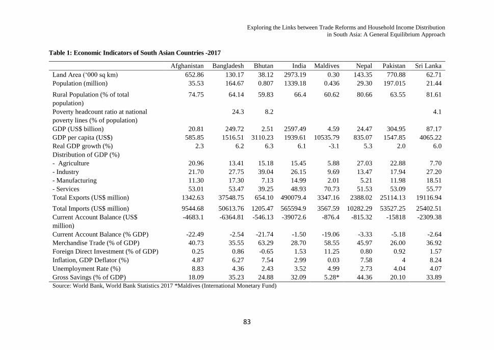
investment flows. Table 1 displays the key economic indicators of the South Asian

Economies. The South Asian region is tremendously diverse in terms of country size,

economic and social development, geography, political systems, languages, and cultures.

The region consists of a single large country, India, surrounded by a number of medium

and small nations including Pakistan, Afghanistan, Bangladesh, Nepal, Bhutan, Sri Lanka

and Maldives. India’s dominance is obvious, accounting for more than 79% of the

region’s GDP and 73%of its population in 2017. It also commands a leading position in

international trade while having relatively low trade openness (35.5%) with the rest of the

world. The World Bank classifies India, Sri Lanka, Maldives and Bhutan as lower middle-

income countries (LMC) and the other four South Asian countries as low-income

countries (LIC).

Among the member countries, Bangladesh, India, and Pakistan, which account for 95%

of the region’s population, the range of per capita income was narrower: US$ 585 in

Afghanistan, US$ 1547 in Pakistan, US$ 4065 in Sri Lanka and US$ 1939 in India.

Today, South Asia as a region is generally characterised by low per capita incomes, a

high incidence of poverty and poor infrastructure.

Trends in Economic Growth and Sectoral Composition of GDP

According to the Asian Development Outlook, 2017 it is noticed that, despite the slight

fall in developing Asia’s growth forecast overall, the South Asia’s economic growth

remains impressive over the period of 2000-2017.



83

Table 1: Economic Indicators of South Asian Countries -2017

Afghanistan Bangladesh Bhutan India Maldives Nepal Pakistan Sri Lanka

Land Area (‘000 sq km) 652.86 130.17 38.12 2973.19 0.30 143.35 770.88 62.71

Population (million) 35.53 164.67 0.807 1339.18 0.436 29.30 197.015 21.44

Rural Population (% of total

population)

74.75 64.14 59.83 66.4 60.62 80.66 63.55 81.61

Poverty headcount ratio at national

poverty lines (% of population)

24.3 8.2 4.1

GDP (US$ billion) 20.81 249.72 2.51 2597.49 4.59 24.47 304.95 87.17

GDP per capita (US$) 585.85 1516.51 3110.23 1939.61 10535.79 835.07 1547.85 4065.22

Real GDP growth (%) 2.3 6.2 6.3 6.1 -3.1 5.3 2.0 6.0

Distribution of GDP (%)

- Agriculture

- Industry

- Manufacturing

- Services

20.96

21.70

11.30

53.01

13.41

27.75

17.30

53.47

15.18

39.04

7.13

39.25

15.45

26.15

14.99

48.93

5.88

9.69

2.01

70.73

27.03

13.47

5.21

51.53

22.88

17.94

11.98

53.09

7.70

27.20

18.51

55.77

Total Exports (US$ million) 1342.63 37548.75 654.10 490079.4 3347.16 2388.02 25114.13 19116.94

Total Imports (US$ million) 9544.68 50613.76 1205.47 565594.9 3567.59 10282.29 53527.25 25402.51

Current Account Balance (US$

million)

-4683.1 -6364.81 -546.13 -39072.6 -876.4 -815.32 -15818 -2309.38

Current Account Balance (% GDP) -22.49 -2.54 -21.74 -1.50 -19.06 -3.33 -5.18 -2.64

Merchandise Trade (% of GDP) 40.73 35.55 63.29 28.70 58.55 45.97 26.00 36.92

Foreign Direct Investment (% of GDP) 0.25 0.86 -0.65 1.53 11.25 0.80 0.92 1.57

Inflation, GDP Deflator (%) 4.87 6.27 7.54 2.99 0.03 7.58 4 8.24

Unemployment Rate (%) 8.83 4.36 2.43 3.52 4.99 2.73 4.04 4.07

Gross Savings (% of GDP) 18.09 35.23 24.88 32.09 5.28* 44.36 20.10 33.89

Source: World Bank, World Bank Statistics 2017 *Maldives (International Monetary Fund)


84

From 2000 to 2017, the region’s GDP grew at about 6% annually – nearly twice the rate of the

world economy (World Trade Organisation, 2017). Increased globalisation and the opening up

of South Asian markets to the rest of the world were important features, particularly since

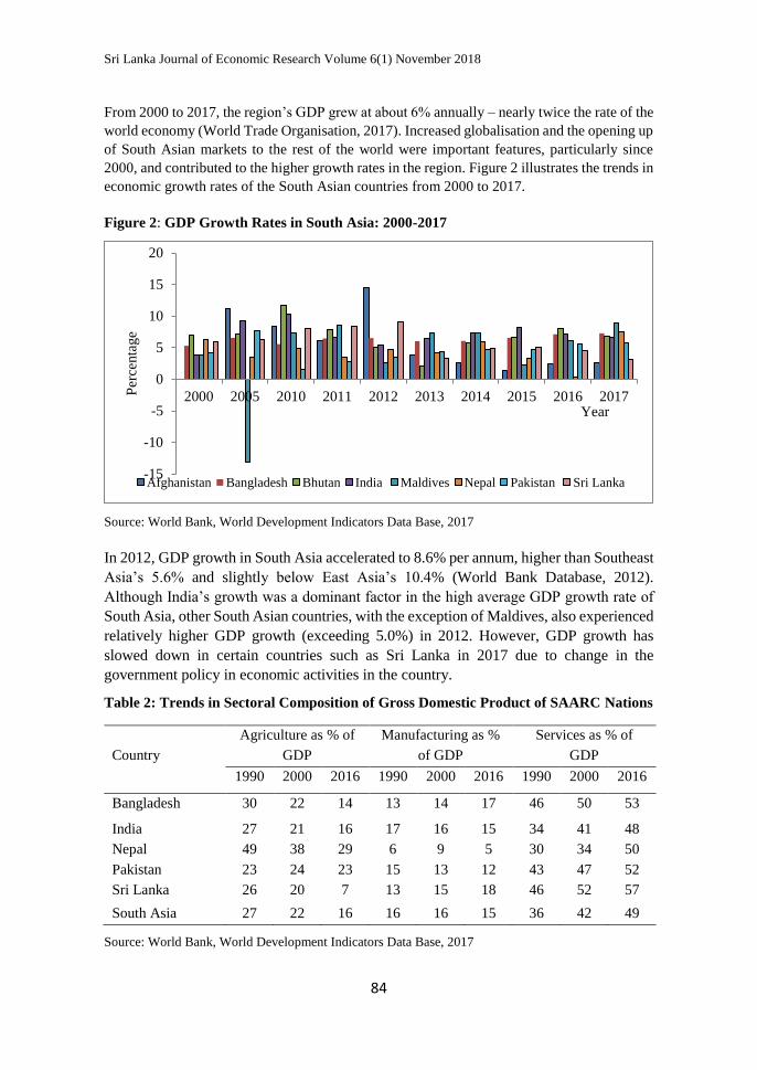
2000, and contributed to the higher growth rates in the region. Figure 2 illustrates the trends in

economic growth rates of the South Asian countries from 2000 to 2017.

Figure 2: GDP Growth Rates in South Asia: 2000-2017

Source: World Bank, World Development Indicators Data Base, 2017

In 2012, GDP growth in South Asia accelerated to 8.6% per annum, higher than Southeast

Asia’s 5.6% and slightly below East Asia’s 10.4% (World Bank Database, 2012).

Although India’s growth was a dominant factor in the high average GDP growth rate of

South Asia, other South Asian countries, with the exception of Maldives, also experienced

relatively higher GDP growth (exceeding 5.0%) in 2012. However, GDP growth has

slowed down in certain countries such as Sri Lanka in 2017 due to change in the

government policy in economic activities in the country.

Table 2: Trends in Sectoral Composition of Gross Domestic Product of SAARC Nations

Country

Agriculture as % of

GDP

Manufacturing as %

of GDP

Services as % of

GDP

1990 2000 2016 1990 2000 2016 1990 2000 2016

Bangladesh 30 22 14 13 14 17 46 50 53

India 27 21 16 17 16 15 34 41 48

Nepal 49 38 29 6 9 5 30 34 50

Pakistan 23 24 23 15 13 12 43 47 52

Sri Lanka 26 20 7 13 15 18 46 52 57

South Asia 27 22 16 16 16 15 36 42 49


-15

-10

-5

0

5

10

15

20

2000 2005 2010 2011 2012 2013 2014 2015 2016 2017Per

centa

ge

Year

Afghanistan Bangladesh Bhutan India Maldives Nepal Pakistan Sri Lanka



85

Table 2 above illustrates the trends in sectoral composition of GDP in South Asia from

1990-2016. What is immediately noticeable is the remarkable increase in the service

sector in all South Asian economies over the period. Although the share of agriculture to

GDP declined from 27% in 1990 to 16% in 2016, it is worth noting that the agricultural

sector continues to play a very important role in South Asia as nearly 55% of the labour

force is engaged in this sector in South Asia (World Bank, 2017).

Trends in External Trade and Average Tariff in South Asia

South Asia was a relatively protected region in the 1950s, with countries imposing high

tariff barriers to foster industrial development through import-substitution policies. By the

early 1990s, however, all of the countries within the region had begun implementing

liberalisation policies, and six of the South Asian countries namely; Bangladesh, India,

Maldives, Nepal, Pakistan and Sri Lanka remain committed to freer multilateral trade as

World Trade Organisation (WTO) members. Consequently, South Asian international

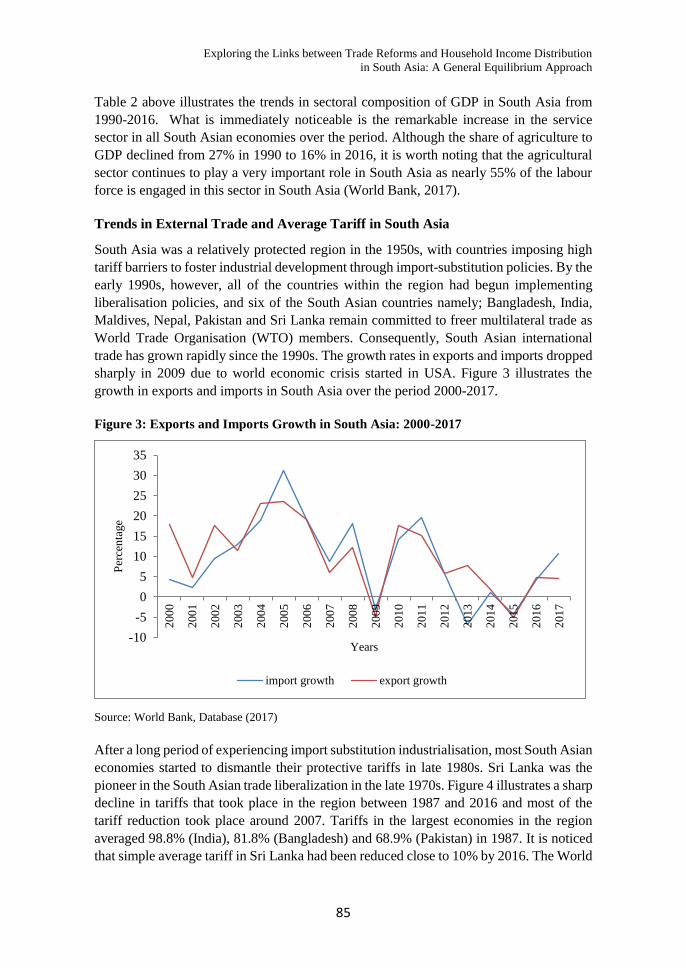
trade has grown rapidly since the 1990s. The growth rates in exports and imports dropped

sharply in 2009 due to world economic crisis started in USA. Figure 3 illustrates the

growth in exports and imports in South Asia over the period 2000-2017.

Figure 3: Exports and Imports Growth in South Asia: 2000-2017

Source: World Bank, Database (2017)

After a long period of experiencing import substitution industrialisation, most South Asian

economies started to dismantle their protective tariffs in late 1980s. Sri Lanka was the

pioneer in the South Asian trade liberalization in the late 1970s. Figure 4 illustrates a sharp

decline in tariffs that took place in the region between 1987 and 2016 and most of the

tariff reduction took place around 2007. Tariffs in the largest economies in the region

averaged 98.8% (India), 81.8% (Bangladesh) and 68.9% (Pakistan) in 1987. It is noticed

that simple average tariff in Sri Lanka had been reduced close to 10% by 2016. The World

-10

-5

0

5

10

15

20

25

30

35

200

0

200

1

200

2

200

3

200

4

200

5

200

6

200

7

200

8

200

9

201

0

201

1

201

2

201

3

201

4

201

5

201

6

201

7

Per

cen

tage

Years

import growth export growth


86

Bank (2018) pointed out that trade liberalisation in South Asia has not been smooth.

Several countries in South Asia have implemented trade reforms over the last two decades;

Bangladesh in the late 1990s and Pakistan and Sri Lanka after the global financial crisis

in the late 2000s. The World Bank (2018) indicates that, despite the trade reforms, tariffs

in South Asian economies are still higher compared with those in other regions. In 2016,

the simple average tariffs in South Asia was 13.6%, which is more than double the world

average (6.3%) and the highest among major regions in the world. For instance, the simple

average tariffs in North America is 2.7%; Europe and Central Asia, 4.3%; East Asia and

Pacific, 7.3%; Latin America and Caribbean, 7.4% and Sub-Saharan Africa, 11.4%. This

clearly demonstrates that, it is important for South Asian economies to initiate steps to

further liberalise their economies.

Figure 4: Simple Average Tariffs in South Asia: 1987-2016

Source: World Trade Organisation (WTO), United Nation Conference on Trade and Development

(UNCTAD) database (2017).

Poverty and Income Distribution in South Asia

South Asia is one of the poorest regions in the world and, after Sub-Saharan Africa, is

home to the largest concentration of the world population living in poverty. Despite more

rapid economic growth in South Asia in the recent years, the region is still home to about

596 million of the 912 million poor living in the Asia and Pacific region (The World Bank,

2010). Figure 5 illustrates that South Asia has experienced a substantial reduction in both

the incidence of poverty and the absolute number of poor over the period 2005 to 2016.

Poverty in the South Asian region has fallen from 33.6% in 2005 to about 15.1% in 2016.

Most countries have made progress in poverty reduction following trade liberalisation in

the region in the 1990s.

0

20

40

60

80

100

120

Per

cen

tage

Country

1987 1997 2007 2016



87

Figure 5: The Share of Working Poor Living on less than US$ 1.90 per Day by Region


Figure 6 (a) and 6(b) below depict the patterns of income distribution in South Asia.

Figures 6(a) demonstrates the income share held by the richest 20% and the poorest 20%

of the total working population while Figure 6(b) illustrates the income share held by the

richest 10% and the poorest 10% of the total working population in the South Asian

countries.

Figure 6 (a): Income Share held by Poorest and the Richest 20% of the total Population

18.4

5

10.8

3

33.6

50

3.5 2.25.4

15.1

41

0

10

20

30

40

50

60

East Asia and

Pacific

Europe and

Central Asia

Latin America

and caribbean

Middle East

and North

Africa

South Asia Sub-Saharan

Africa

Per

cen

tage

Region

2005 2016


88

Figure 6(b): Income Share held by Poorest and the Richest 10% of the Population


Survey Years: Sri Lanka 2007, Pakistan 2006, India 2005, Nepal 2004 and Bangladesh 2005,

Bhutan 2003 and Afghanistan 2008.

Under both circumstances, the gap is the largest in Nepal followed by Bhutan, Sri Lanka

and India. In examining Figures 6(a) and 6(b) it is evident that even though there has been

a decline in overall poverty in the South Asian region, income inequality between the rich

and poor has widened among the countries in the region.

The Model and Data

To analyse the effects of trade liberalisation in South Asia, a static multi-country CGE

model for South Asia (SAMGEM) is formulated which links country or regional models

all over the world through trade and investment. Its framework and database are basically

the same as the GTAP (Global Trading Analysis Project) model. An important feature of

the SAMGEM, which makes it different from the ‘standard’ GTAP model is that it

attempts to incorporate a multi-household11 dimension into the model. Accordingly, the

household sector is disaggregated based on different income groups in different

geographical regions of four countries in South Asia (India, Sri Lanka, Bangladesh and

Pakistan). The equations in SAMGEM are written using the TABLO language in the

GEMPACK (General Equilibrium Modelling Package) software. The principal

programming language for GTAP data and modelling work is based on the GEMPACK

software which is capable of handling complex linear, nonlinear and mixed integer

optimization problems (Harrison & Pearson, 1996).

11 In the standard GTAP model each region has a single representative household (Hertel & Tsigas,

1997).



89

Database

The data for SAMGEM are mainly taken from the GTAP database version 7, which

reflects the world economy in 2004 (Narayanan & Walmsley, 2008). The data are

aggregated into sixteen regions, thirty sectors and three primary factors. The GTAP

version 7 contains 113 countries/regions and in designing the model 113 countries/regions

have been aggregated into 16 countries/regions (Appendix A.1). In formulating the model,

57 GTAP sectors have been aggregated into 30 sectors (Appendix A.2). The five factors

in the GTAP model have been aggregated into the three factors, namely; skilled labour,

unskilled labour and capital (including land and natural resources) with each group

assumed to be homogeneous. The factor aggregation of the model is presented in

Appendix A.3. In SAMGEM one representative household is specified for the rest of the

world other than the above mentioned four South Asian countries. For these four South

Asian countries, the household sector is disaggregated according to different income

classes based on different geographical classifications. For instance, in the case of Sri

Lanka the household sector is disaggregated into 30 household groups according to

income deciles and geographical regions consisting of 10 rural groups, 10 urban groups

and 10 estate sector12 groups. In India, the household sector is disaggregated into 24

household groups according to monthly per capita consumer expenditure (MPCE) classes

consisting of 12 rural groups and 12 urban groups. In Pakistan, the household sector is

disaggregated into 10 household groups according to income quintiles consisting of 5 rural

groups and 5 urban groups. In the case of Bangladesh, the household sector is

disaggregated based on MPCE. Accordingly, the household sector includes a total of 38

groups, consisting of 19 rural and 19 urban groups.

To evaluate the economic impacts of trade liberalisation in South Asia on household

income distribution, additional data on household income and expenditure are used for the

four South Asian countries. These data are compiled by the Central Bank of Sri Lanka

(which conducted the Consumer Finances and Socio Economic Survey in 2003/2004), the

National Sample Survey Organisation (NSSO) of India (which conducted the Household

Expenditure Survey in 2004), the Federal Bureau of Statistics of Pakistan (which

conducted the Household Income and Expenditure Survey in 2004/2005) and Bangladesh

Bureau of Statistics (which conducted the Household Income and Expenditure Survey in

2004/2005). The household data for 2003/2004 and 2004/2005 for the South Asian

countries are used as it is consistent with the 2004 base year in version 7 of the GTAP

database. The commodity groups in the household survey data of each of the South Asian

countries are matched and categorised under the 30 industries aggregated from the GTAP

database. Further, the household income is proportionally allocated among different

factors of the GTAP based on the proportions calculated from the household survey data

12 The estate sector is considered to be part of the rural sector. Large plantations growing tea, rubber and

coconut were introduced in Sri Lanka during the British colonial period and labour was imported from

South India to work on these plantations. These are included in the estate sector which comprises 5 per

cent of the total population in Sri Lanka (World Bank, 2009).


90

of the respective South Asian economies depending on the sources of income received by

the households.

In modelling the government sectors the data for government budget deficits/surpluses

and net foreign transfers were obtained from the International Financial Statistics Year

Book (2004), for all the countries presented in Appendix A.1. In addition, it should be

noted that the choice of elasticity values critically affects the results of policy simulations

generated by the model and hence, it is important to select appropriate values for these

parameters. Most of the elasticity values applied in the model were directly taken from

version 7 of the GTAP database. Moreover, the income or expenditure elasticity values

for different household groups have been obtained from previous studies undertaken for

South Asian countries (Rajapakse, 2011; Majumder, 1986; Yen & Roe, 1986; Burney &

Khan, 1991).

Construction of the Model

The modelling of each region in the standard GTAP is based on the ORANI model (Dixon

et al., 1982) and imposes the assumptions of constant returns to scale in production and

perfect competition in commodity and factor markets.

In SAMGEM each regional household (private household and the government) owns the

factors of production. Private household income consists of labour and capital income,

and income is allocated to savings and consumption using exogenous shares. Households

of the four South Asian countries receive fixed proportions of sectoral capital income

based on their initial supplies of capital services. Labour income is defined as wages and

salaries, whereas capital income is profit from household investment and income from

land and natural resources. Labour income is determined by the household supply of

labour in each industry and the corresponding wage rates. The household composition of

sectoral labour income would change as labour moves between industries during the trade

liberalisation.

Household disposable income is total income less income taxes and private household

savings. The household consumption demand is determined using the Linear Expenditure

System (LES) function. This is one of the key differences between GTAP and SAMGEM,

as in the GTAP model household consumption is determined using a Constant Difference

Elasticity (CDE) function. In modelling the household consumption equations, the

ORANI-G multi-household framework has been followed (Centre of Policy Studies, of

the Monash University, 2004). The LES function is used in the SAMGEM because it can

measure the effect of a change in income on the structure of the consumption. In the model,

households make the optimal allocation between consumption of commodities by

maximisation of the Stone Geary Utility function or LES function subject to its budget

constraint, which is the disposable income spent on consumption.

The government in each region is an institutional sector and acts as a consumer. It receives

revenue from taxes and tariffs. Eight kinds of taxes and subsidies were specified in each

country model consisting of tariffs, export duties, production taxes and output subsidies,

taxes on intermediate inputs, sales taxes imposed on consumer goods and public goods,



91

factor taxes and income taxes. Government revenue consists of revenues from all taxes,

foreign grants and transfers from households, and is allocated among consumption and

government savings. All the equations relating to production, investment, transportation

and trade in SAMGEM are based on the standard GTAP model.

Policy Experiment and Model Closure

The policy simulation mentioned below is analysed in both short run and long run

frameworks. In the short run real wages are held fixed, with employment adjusting in each

industry. In the capital market the capital stock in each sector is held fixed, with rates of

return to capital adjusting endogenously. Further, the trade balance is fixed, with real

consumption, investment and government spending moving together to accommodate it

(Horridge, 2000).

However, if the time frame under consideration is deemed to be long run in nature, capital

stock is allowed to vary while labour supply is assumed to be fixed. This reflects that

capital can adjust over time with the natural rate of unemployment. Under this scenario

the price of labour is allowed to vary while the price of capital remains fixed. In addition,

the trade balance, real consumption, government consumption and investments become

endogenous in the model. Since the model can only be solved for (n-1) prices, one price

is set exogenously, and all other prices are evaluated relative to this numéraire

(Brockmeier, 2001). Accordingly, as in the standard GTAP the global average return to

primary factors is used as the numéraire in the model.

South Asia Free Trade Area (SAFTA)

Since, all South Asian economies are committed to reduce all tariff barriers by at the

implementation of SAFTA, this simulation considers full implementation of the SAFTA

in its originally proposed form where all SAARC countries reduce their existing tariff

rates to 0% among all members in South Asia while maintaining the existing tariffs

barriers with the rest of the world.

Furthermore, in undertaking the above mentioned simulations it is assumed that non-tariff

barriers are absent. This is a realistic assumption as the WTO notified that all the

developing countries are required to eliminate their non-tariff barriers post 2005.

Simulation Results

Trade policy analysts are concerned with the overall economic benefits that the country

will receive in the event that free trade treaties are successfully negotiated (Siriwardana &

Yang, 2007). On the basis of model simulation this section reports the results of the

estimated short run and long run impacts of trade liberalisation on the important

macroeconomic variables, trade, household income, government revenue and the

economic welfare of the South Asian economies. The level of welfare is determined based

on the equivalent variation (EV) that arises under the policy simulation.


92

Impact of Trade Liberalisation on Macroeconomic Variables

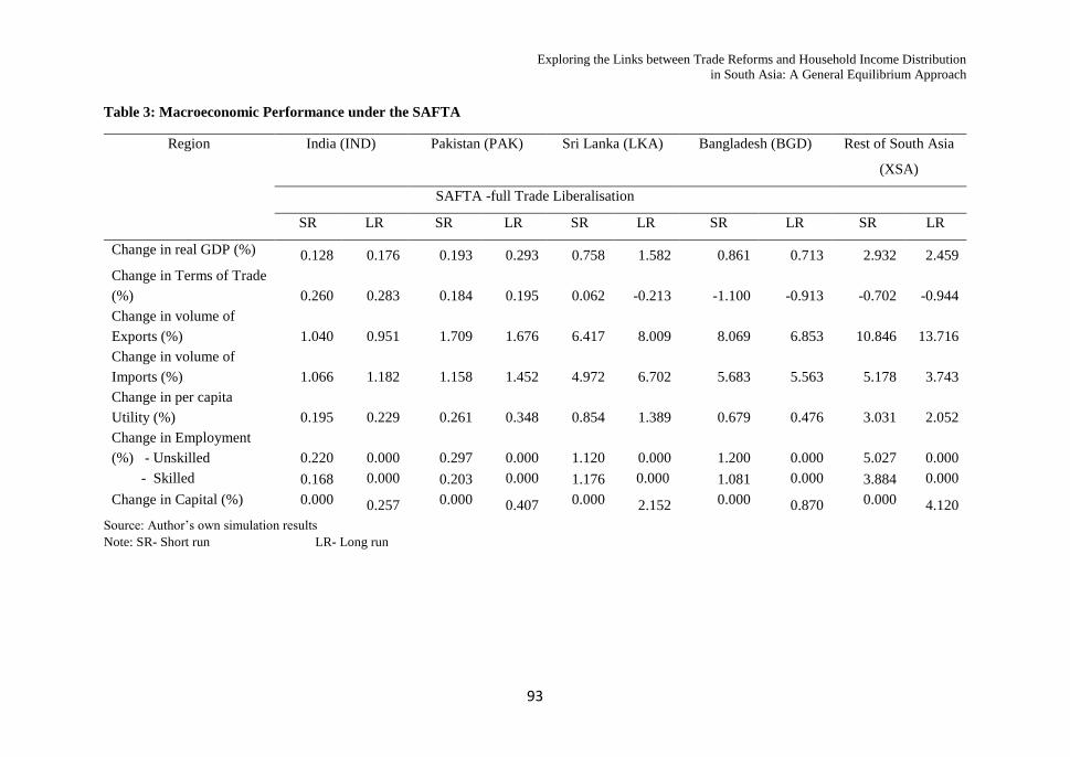
The macroeconomic effects of trade liberalisation in South Asia are illustrated in the Table

3 below. The table compares both short run and long run macroeconomic implications of

the implementing SAFTA. Several important points emerged from these projections. The

results indicate that under the SAFTA there are positive impacts on real GDP in all South

Asian economies in the short run as well as in the long run. Another point to be noted is

that the gains in GDP are higher in the long run for each South Asian economy, except in

the Rest of South Asia and Bangladesh, as a result of better utilisation of capital. Further,

the results illustrate that there is higher increase in employment in labour (especially

unskilled labour) with the implementation of the SAFTA. Hence, liberalisation labour

intensive industries such as agriculture is important for South Asia as the agricultural

sector continues to play a significant role in terms of employment to a vast majority of the

labour force in the region.

There is an improvement in the terms of trade in all countries, except in Bangladesh and

the Rest of South Asia in the short run. However, Sri Lanka’s terms of trade deteriorates

in the long run under the SAFTA as result of a decrease in export prices relative to import

prices. It seems that in the long run trade liberalisation would result in Sri Lanka losing

export competitiveness in the international market, as Sri Lanka competes with larger

economies in the region such India and Pakistan. Since, all South Asian economies export

and import similar products, for example textiles and wearing apparel, larger economies

gain greater competitive power than the smaller economies in the region.

Impact of Trade Liberalisation on Sectoral Trade

Table A.4 in the appendix illustrates the percentage changes in total sectoral exports and

imports of the South Asian countries under the SAFTA. Under the SAFTA when all tariffs

have been eliminated, exports and imports of agricultural products increase more than

manufacturing goods in all South Asian countries both in the short run and in the long run.

The results suggest that under this policy option there is an increase in the exports of

textiles from all South Asian countries in the short run and the long run. This is because

South Asia has a natural advantage in the production of textile yarn and fabric, producing

the bulk of the world’s cotton which is the most important raw material for the industry.

Since, the region also has an abundance of cheap labour to work in this industry, it is

advantageous for textile entrepreneurs in South Asia to modernise their plants to be

competitive with the other textile manufacturers in the world. It seems that in most of the

South Asian economies the wearing apparel sector is not benefiting from the phasing out

of the quota regime in 2005. Yet, the results suggest that in Bangladesh there is a rise in

exports of wearing apparel (9.42% in the short run 8.23% in the long run) and being a

least developed country in the region Bangladesh still continues to enjoy tariff preferences

in major markets (United States Agency for International Development Research Group,

2005).



93

Table 3: Macroeconomic Performance under the SAFTA

Source: Author’s own simulation results

Note: SR- Short run LR- Long run

Region India (IND) Pakistan (PAK) Sri Lanka (LKA) Bangladesh (BGD) Rest of South Asia

(XSA)

SAFTA -full Trade Liberalisation

SR LR SR LR SR LR SR LR SR LR

Change in real GDP (%) 0.128 0.176 0.193 0.293 0.758 1.582 0.861 0.713 2.932 2.459

Change in Terms of Trade

(%) 0.260 0.283 0.184 0.195 0.062 -0.213 -1.100 -0.913 -0.702 -0.944

Change in volume of

Exports (%) 1.040 0.951 1.709 1.676 6.417 8.009 8.069 6.853 10.846 13.716

Change in volume of

Imports (%) 1.066 1.182 1.158 1.452 4.972 6.702 5.683 5.563 5.178 3.743

Change in per capita

Utility (%) 0.195 0.229 0.261 0.348 0.854 1.389 0.679 0.476 3.031 2.052

Change in Employment

(%) - Unskilled 0.220

0.000 0.297

0.000 1.120

0.000 1.200

0.000 5.027

0.000

- Skilled 0.168 0.000 0.203 0.000 1.176 0.000 1.081 0.000 3.884 0.000

Change in Capital (%) 0.000 0.257 0.000 0.407 0.000 2.152 0.000 0.870 0.000 4.120


94

It is noticed that the member countries of the SAFTA agreement retain Most Favoured

Nation (MFN) tariff rates for the items included in their sensitive lists which mostly

contain agricultural goods.

Since agricultural goods dominate intra-regional trade in South Asia, the members should

imitate steps to remove such products from the sensitive list as higher tariffs on

agricultural products might seriously inhibit intra-regional trade in the region.

Impact on Household Income

The percentage changes in unskilled labour income, skilled labour income, capital income

(including income on land and natural resources) and government transfers that accrue to

households located in different geographical areas in the respective South Asian countries

are presented in figures A.5 to A.8 in the appendix under the SAFTA. It is noticed that

household income increases in all South Asian countries in the short run as well as in the

long run. However, it should be noted that the long run gains are higher than those of the

short run due to efficient allocation of resources and the creation of more investment

opportunities in the long run.

Under the SAFTA, unskilled labour income in rural households increases proportionately

in all South Asian countries whereas income of skilled labour and capital increase more

in urban households as predicted by the Heckscher-Ohlin (H-O) model. On the other hand

transfers from government to households decline in smaller economies, except in India

and Pakistan, under the SAFTA with zero tariff agreement. In overall it is interesting to

notice that in the long run trade liberalisation would result in a larger narrowing of income

disparities in all South Asian economies than in the short run.

Figure 7: Percentage Change in Government Revenue and Budget Deficit: SAFTA


0.30 0.02 -2.35 -1.67 -3.85 0.38 0.24-1.46 -1.66 -5.52

0.76 2.434.94

16.74

61.75

0.79 1.703.31

19.40

99.03

-20.00

0.00

20.00

40.00

60.00

80.00

100.00

IND PAK LKA BGD XSA IND PAK LKABGD XSA

Short run Long run

Per

cen

tage

Country/Region

Govt. Revenue

Budget Deficit



95

Impact on Government Revenue

The percentage change in total government revenues in the South Asian economies under

the SAFTA is illustrated in Figure 7. The results suggest that elimination of import tariffs

would result in reductions in government revenue in all South Asian economies, except in

India and Pakistan, both in the short run and the long run. There is marginal increase in

total government revenue in India (0.30% in short run and 0.38% in the long run) and in

Pakistan (0.02% in short run and 0.24% in long run). Table A.9 in the appendix explains

in detail the composition of the sources of government revenue and their change (in US$

million) due to trade liberalisation. From the table it is evident that India’s total

government revenue increases as a result of an increase in both indirect taxes as well as

direct taxes. It is interesting to note that under the SAFTA zero tariff agreement there is

still an increase in the revenue from import tariffs in India, as India trades heavily with

other countries outside the region.

Table 4: Equivalent Variation under the SAFTA

Region

SAFTA: full Trade Liberalisation

Short Run

(US$ Million)

Long Run

(US$ Million)

1 IND 1146.579 1344.943

2 PAK 226.940 302.786

3 LKA 152.438 247.888

4 BGD 344.994 241.720

5 XSA 386.156 261.350

6 USA -95.656 -25.371

7 CAN -5.868 -3.294

8 EU -175.055 -43.706

9 ASE -80.309 -39.184

10 HIA -74.300 -36.695

11 JPN -111.382 -28.494

12 CHN -108.980 -60.864

13 XME -75.717 -33.670

14 AUS_NZL -29.773 -11.209

15 RUS_XSU -7.186 -6.521

16 ROW -128.952 -21.140

Total 1363.928 2088.539



96

Welfare impacts of Trade Liberalisation

Equivalent variation (EV) is used to determine the overall level of welfare under each

policy option (Table 4). EV is an absolute monetary measure of welfare improvement in

terms of income that results from the fall in import prices when tariffs are reduced or

eliminated.

The welfare projections indicate that in both the short run and the long run all economies

gain under the SAFTA. Further, it is important to note that although welfare improves in

India, Pakistan, and Sri Lanka in the long run, Bangladesh and Rest of South Asia gain

more in the short run under both policy options. Hence, the long run welfare gains are

lower for least developed economies in the region under the SAFTA.

CONCLUDING REMARKS

This paper analysed the impact of the SAFTA with full trade liberalisation using a multi-

country CGE model formulated for South Asia based on the GTAP model. It is noticed

that the real GDP improves in all South Asian economies under the SAFTA zero tariff

agreement. It is apparent that the gains in real GDP are proportionately higher in the long

run than in the short run in all South Asian economies with the exception of Bangladesh

and Rest of South Asia which are the least developed economies in the region. Although,

it seems that welfare gains for India, Pakistan, and Sri Lanka are likely to increase in the

long run, there are less welfare gains for Bangladesh and the Rest of South Asia in the

long run under the SAFTA.

Industry level results indicate that South Asian countries can encourage trade among

SAFTA members by eliminating barriers, particularly eliminating the products included

in the sensitive lists. The results suggest that there are substantial increases in exports of

agricultural products such as wheat, grains, vegetables and oil seeds, especially in

Bangladesh and Rest of South Asia both in the short run and in the long run. This implies

the member countries should remove both tariff and non-tariff barriers especially in the

agricultural sector by revising their sensitive product lists, as substantial development of

agricultural trade in the region cannot be otherwise envisaged. The World Bank (2018)

noted that in 2015, nine years after implementation of SAFTA had come into force in

2006, about 43.7% of intra-SAARC imports were still restricted under the sensitive list,

which becomes a barrier to boost the intra regional trade in South Asia. The model results

support the view that the trade liberalisation would enhance economic growth which is

the most powerful instrument for reducing poverty and improving the quality of life in

South Asian economies.

Two general qualifications need to be kept in mind when interpreting the results presented

from this analysis. Firstly, the multi-country CGE model used to undertake the

simulations is a static model and hence the dynamic effects of the trade liberalisation are

not captured. Secondly, issues such as bilateral investments and service trade

liberalisation are not considered under the present analysis which can be important areas

for future research concern.



97

REFERENCES

Bourguignon, F., & Spadaro, A. (2006). Microsimulation as a Tool for Evaluating

Redistribution Policies. Journal of Economic Inequality, 4, 77-106.

Narayanan, B. G. & Walmsley, T. L. E. (2008). Global Trade, Assistance, and Production: The

GTAP 7 Data Base. Center for Global Trade Analysis, Purdue University.

Bangladesh Bureau of Statistics. (2004/2005). Household Income and Expenditure Survey.

Brockmeier, M. (2001). A Graphical Exposition of the GTAP Model, GTAP Technical Paper

No. 8, Center for Global Trade Analysis, Purdue University, West Lafayette, Indiana.

Retrieved from www.gtap.org

Burney, N. A., & Khan, A. H. (1991). Household Consumption Pattern in Pakistan: An Urban

Rural Comparison Using Micro Data. The Pakistan Development Review, 30(2), 145-

171.

Centre of Policy Studies, Monash University web page [http//www.monash.edu.au/policy/]

Cockburn, J. (2001). Trade Liberalisation and Poverty in Nepal A Computable General

Equilibrium Micro Simulation Analysis. Retrieved from

[http://www.crefa.ecn.ulaval.ca]

Cogneau, D., & Robilliard, A. S. (2001), Growth Distribution and Poverty in Madagascar:

Learning from a Microsimulation Model in a General Equilibrium Framework, TMD

Discussion Paper 61. In International Food Policy Research Institute, Washington

DC, 2000.

Decaluwé, B., Dumont, J. C., & Savard, L. (1999). Measuring Poverty and Inequality in a

Computable General Equilibrium Model. Québec, Canada: Université Laval.

Dixon, P., Malakellis, M., & Meagher, T. (1995). A Microsimulation/Applied General

Equilibrium Approach to Analysing Income Distribution in Australia: Plans and

Preliminary Illustration. Paper presented at the Industry Commission Conference on

Equity, Efficiency and Welfare, Melbourne.

Dixon, P.B., Parmenter, B. R., Sutton, J. & Vincent, D. P. (1982). ORANI: A Multisectoral

Model of the Australian Economy, Contributions to Economic Analysis 142, North-

Holland Publishing Company.

Dollar, D., & Kraay, A. (2004). Trade, Growth and Poverty. The Economic Journal, 114, F22-

F49.

Evans, D. (June 2001). Identifying Winners and Losers in Southern Africa from Global Trade

Policy Reform: Integrating Findings from GTAP and Poverty Case Studies. Paper

presented at the Fourth Annual Conference on Global Economic Analysis, Purdue

University, West Lafayette.

Ezaki, M., & Nguyen, T. D. (April 2008). Regional Economic Integration and Its impact on

growth, income distribution and Poverty in East-Asia Nagoya: Graduate School of

International Development, Nagoya University, Japan.

http://www.gtap.org/

http://www.crefa.ecn.ulaval.ca/


98

Fiestas, I. (2005). The effects of trade liberalization on growth, poverty and inequality. CILAE

Nota técnica NT/04, 5.

Gerber, J. (1999). International Economics. Addison Wesley Educational Publishers Inc.

Gilbert, J. (2008). Trade policy, poverty, and income distribution in CGE models: an application

to SAFTA. Emerging Trade Issues for Policymakers in Developing Countries in Asia

and the Pacific, UNESCAP: Bangkok.

Gilbert, J., & Oladi, R. (2010). Regional Trade Reform Under SAFTA and Income Distribution

in South Asia. Frontiers of Economics and Globalization: New Developments in

Computable General Equilibrium Analysis of Trade Policy 7.

Harrison, W. J., & Pearson, K. R. (1996). Computing solutions for large general equilibrium

models using GEMPACK. Computational Economics, 9(2), 83-127.

Hertel, T. W., & Reimer, J. (2005). Predicting the Poverty Impacts of Trade Reform. Journal of

International Trade & Economic Development, 14(4), 377 – 405.

Hertel, T. W., & Tsigas, M. E. (1997). Global Trade Analysis: Modelling and Applications:

Cambridge University Press.Ianchovichina, E., Nicita, A., & Soloaga, I. (2002).

Trade Reform and Poverty: The Case of Mexico. The World Economy, 25(7), 945–

972.

Hertel, T. W., Ivanic, M., Preckel, P. V., & Cranfield, J. A. (2003). The earnings effects of

multilateral trade liberalization: implications for poverty. The World Bank Economic

Review, 18(2), 205-236.

Horridge, M. (2000). ORANI-G: A generic single-country computable general equilibrium

model. CoPS Working. Paper OP-93, Centre of Policy Studies, Monash University

Majumder, A. (April, 1986). Consumer Expenditure Pattern in India: A Comparison of the

Almost Ideal Demand Systemand the Linear Expenditure System. The Indian Journal

of Statistics, 48 (1), 115-143.

Meagher, G. A. (1996). Forecasting changes in the distribution of income: an applied general

equilibrium approach, in Harding, A. Microsimulation and Public Policy, 361–384.

Naranpanawa, R. M. A. K. B. (2005). Trade liberalization and poverty in a computable general

equilibrium (CGE) model: the Sri Lankan case. Unpublished PhD Thesis. Griffith

Business School, Griffith University.

Rajapakse, S. (February 2011). Estimation of a complete system of nonlinear Engel curves:

further evidence from Box–Cox Engel curves for Sri Lanka. Applied Economics, 43,

371–385.

Reimer, J. (2002). Estimating the Poverty Impacts of Trade Liberalization: Center for Global

Trade Analysis and Department of Agricultural Economics, Purdue University,

U.S.A.

Savard, L. (2004). Poverty and inequality analysis within a CGE framework: A comparative

analysis of the representative agent and microsimulation approaches. Development

Policy Review, 23(3), 313-331.



99

Sawhney, A., & Kumar, R. (2008). Rejuvenating SAARC: The strategic payoffs for

India. Global Economy Journal, 8(2).

Selim, R. (2010). Welfare and Poverty Impacts of Trade Liberalization: A Dynamic CGE

Microsimulation Analysis. International Journal of Microsimulation, 3(1), 123-126.

Siriwardana, M., & Yang, J. (2007). Economic effects of the proposed Australia-China free

trade agreement. Center for Contemporary Asian Studies, Doshisha University

Working Paper, (4).

Sothea, O. (2009). Income Distribution and Poverty in a CGE Framework: A Proposed

Methodology. PhD, Monash University, Melbourne, Australia.

The Central Bank of Sri Lanka. (2003/2004). Consumer Finance and Socio-Economic Survey

Colombo: The Central Bank of Sri Lanka.

The Federal Bureau of Statistics of Pakistan, Household Income and Expenditure Survey

(2004/2005)

The National Sample Survey Organisation (NSSO) of India, Household Expenditure Survey

(2004)

The World Bank. (2005, 2008, 2009, 2010 & 2017). The World Bank World Development

Report Washington DC: The World Bank.

United States Agency for International Development Research Group. (2005). South Asian Free

Trade Area, Opportunities and Challenges. Retrieved from [http://pdf.usaid.gov]

Whalley, J. (1975). How reliable is partial equilibrium analysis? The Review of Economics and

Statistics, 299-310.

Winters, L. A. (2004). Trade liberalisation and economic performance: An overview. The

Economic Journal, 114(493), F4-F21.

Winters, A. L., McCulloch, N., & Mckay, A. (2004). Trade Liberalization and Poverty: The

Evidence so. Journal of Economic Literature, 42(1), 72-115.

World Trade Organisation (2017). United Nation Conference on Trade and Development

(UNCTAD) Database.

World Trade Organisation. (2017). World Trade Report.

Yen, T., & Roe, T. L. (July, 1986). Determinants of Rural and Urban Household Demand: An

Analysis of Dominican Household Consumption (Vol. 86): Economic Development

Center Department of Economics, Minneapolis.

http://pdf.usaid.gov/


100

Appendix

Table A.1: Regional Aggregation of the GTAP Database

No GTAP

Code

Aggregated

Region

Member Regions

1 IND India India (IND)

2 LKA Sri Lanka Sri Lanka (LKA)

3 PAK Pakistan Pakistan (PAK)

4 BGD Bangladesh Bangladesh (BGD)

5 XSA Rest of South

Asia

Bhutan, Maldives ,Nepal and Afghanistan (XSA)

6 USA United States

of America

United States of America (USA)

7 CAN Canada Canada (CAN)

8 EU European

Union

Austria (AUT) ,Belgium (BEL) ,Denmark (DNK) ,

Finland (FIN) ,France (FRA) ,Germany (DEU) ,United

Kingdom (GBR) ,Greece (GRC) ,Ireland (IRL) ,Italy

(ITA) ,Luxembourg (LUX) ,Netherlands (NLD) ,

Hungary (HUN), Portugal (PRT) ,Spain (ESP) ,Sweden

(SWE), Cyprus(CYP), Czech Republic (CZE),

Estonia(EST), Latvia (LVA), Lithuania (LTU), Malta

(MLT), Poland (POL), Slovakia (SVK) and Slovenia

(SVN).

9 ASE ASEAN Indonesia(IDN),Malaysia (MYS) ,Philippines (PHL) ,

Singapore (SGP) ,Thailand (THA), Vietnam (VNM),

Cambodia (KHM), Lao People's Democratic Republic

(LAO), Myanmar (MMR), Rest of Southeast Asia

(XSE).

10 HIA High Income

Asia

Hong Kong (HKG) ,Korea (KOR) and Taiwan (TWN)

11 JPN Japan Japan(JPN)

12 CHN China China (CHN)

13 XME Rest of

Middle East

Bahrain ,Iran (IRN), Islamic Republic of Iraq, Israel,

Jordan, Kuwait, Lebanon, Oman, Qatar, Saudi Arabia,

Syrian Arab Republic, United Arab Emirates and

Yemen

14 AUS_

NZL

Australia &

New Zealand

Australia(AUS) and New Zealand (NZL)

https://www.gtap.agecon.purdue.edu/databases/IO/table_display.asp?IO_ID=165














101

Table A.1 (Continued….)

No GTAP

Code

Aggregated

Region

Member Regions

15 RUS_

XSU

Russian

Federation

and Rest of

Soviet

Union

Russian Federation (RUS) and Rest of Former Soviet

Union(XSU)

16 ROW Rest of the

World

Rest of Oceania(XOC) , Rest of East Asia (XEA), Mexico

(MEX), Rest of North America (XNA), Argentina (ARG),

Bolivia (BOL), Brazil (BRA), Chile (CHL), Colombia

(COL), Ecuador (ECU), Paraguay (PRY), Peru (PER),

Uruguay (URY), Venezuela (VEN), Rest of South

America (XSM), Costa Rica (CRI), Guatemala (GTM),

Nicaragua (NIC), Panama (PAN), Rest of Central America

(XCA), Caribbean (XCB), Switzerland(CHE), Norway

(NOR), Albania (ALB), Bulgaria (BGR), Rest of EFTA

(XEF), Belarus (BLR), Croatia (HRV), Romania (ROU),

Ukraine (UKR), Rest of Eastern Europe (XEE), Rest of

Europe (XER), Kazakhstan (KAZ), Kyrgyzstan (KGZ),

Armenia (ARM), Azerbaijan (AZE), Georgia (GEO),

Turkey (TUR), Rest of Western Asia (XWE), Egypt

(EGY), Morocco (MAR), Tunisia (TUN), Rest of North

Africa (XNF), Nigeria (NGA), Senegal (SEN), Rest of

Western Africa (XWF), Rest of Central Africa (XCF),

Rest of South Central Africa (XAC), Ethiopia (ETH),

Madagascar (MDG), Malawi (MWI), Mauritius (MUS),

Mozambique (MOZ), Tanzania (TZA), Uganda (UGA),

Zambia (ZMB), Zimbabwe (ZWE), Rest of Eastern Africa

(XEC), Botswana (BWA), South Africa (ZAF) and Rest

of South African Customs Union (XSC).

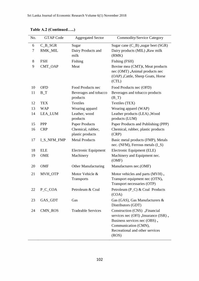
Table A.2: Commodity Aggregation of the GTAP database

No. GTAP Code Aggregated Sector Commodity/Service Category

1 PDR_ PCR Rice; Paddy and

Processed

Paddy rice (PDR) ,Processed rice

(PCR)

2 WHT_GRO Wheat, Cereal Grains Wheat (WHT), Cereal Grains nec

(GRO)

3 V_F Vegetables and fruits Vegetables, fruit, nuts (V_F)

4 OSD_VOL Oil seeds and

vegetable oil

Oil seeds (OSD) ,Vegetable oils and

fats (VOL)

5 PFB_OCR Plant based fibers and

crops

Plant-based fibers (PFB) ,Crops nec

(OCR)








































102

Table A.2 (Continued…..)


6 C_B_SGR Sugar Sugar cane (C_B) ,sugar beet (SGR)

7 RMK_MIL Dairy Products and

milk

Dairy products (MIL) ,Raw milk

(RMK)

8 FSH Fishing Fishing (FSH)

9 CMT_OAP Meat Bovine mea (CMT)t, Meat products

nec (OMT) ,Animal products nec

(OAP) ,Cattle, Sheep Goats, Horse

(CTL)

10 OFD Food Products nec Food Products nec (OFD)

11 B_T Beverages and tobacco

products

Beverages and tobacco products

(B_T)

12 TEX Textiles Textiles (TEX)

13 WAP Wearing apparel Wearing apparel (WAP)

14 LEA_LUM Leather, wood

products

Leather products (LEA) ,Wood

products (LUM)

15 PPP Paper Products Paper Products and Publishing (PPP)

16 CRP Chemical, rubber,

plastic products

Chemical, rubber, plastic products

(CRP)

17 I_S_NFM_FMP Metal Products Basic metal products (FMP), Metals

nec. (NFM), Ferrous metals (I_S)

18 ELE Electronic Equipment Electronic Equipment (ELE)

19 OME Machinery Machinery and Equipment nec.

(OMF)

20 OMF Other Manufacturing Manufactures nec.(OMF)

21 MVH_OTP Motor Vehicle &

Transports

Motor vehicles and parts (MVH) ,

Transport equipment nec (OTN),

Transport necessaries (OTP)

22 P_C_COA Petroleum & Coal Petroleum (P_C) & Coal Products

(COA)

23 GAS_GDT Gas Gas (GAS), Gas Manufacturers &

Distributors (GDT)

24 CMN_ROS Tradeable Services Construction (CNS) ,Financial

services nec (OFI) ,Insurance (ISR) ,

Business services nec (OBS) ,

Communication (CMN),

Recreational and other services

(ROS)



103

Table A.2 (Continued…..)


25 OSG_DWE Non Tradeable

Services

Public Administration, Defense,

Education, Health (OSG) and

Dwellings (DWE)

26 WOL_ NMM Other Primary

products

Wool, Silk worm, cocoons (WOL),

Minerals nec. (OMN), Mineral

product necessaries

27 TRD_CNS Trade & Construction Trade (TRD) & Construction

28 ELY_WTR Electricity, water and

air transport

Electricity (ELY), Water (WTR),

Water transport (WTP), and Air

transport (ATP)

29 OIL Oil Oil (OIL)

30 FRS Natural Resources and

Extracts

Forestry (FRS)

Table A.3: Factor Aggregation

No GTAP Code Description Aggregated Factors

1 UnSkLab Unskilled Labour Unskilled Labour (UnSkLab)

2 SkLab Skilled Labour Skilled Labour (SkLab)

3 Capital Capital Capital (Capital), Land (Land), and

Natural Resources (NatlRes)


104

Table A.4: Change in Sectoral Exports and Imports under the SAFTA

Sector

Exports (% Change) Imports (% Change)

Short Run (% Change) Long Run (% Change) Short Run (% Change) Long Run (% Change)

IND

PAK LKA BGD XSA IND PAK LKA BGD XSA IND PAK LKA BGD XSA IND PAK LKA BGD XSA

1 pdr_pcr 11.79 1.51 -1.50 3.44 1.19 11.47 1.59 0.60 3.55 4.73 1.62 21.52 72.99 56.73 0.13 11.47 1.59 0.60 3.55 4.73

2 wht_gro 1.95 9.41 -0.92 116.35 7.27 2.11 9.30 1.00 116.04 8.27 1.12 0.94 3.55 3.49 3.26 2.11 9.30 1.00 116.04 8.27

3 v_f 5.21 18.27 20.49 5.54 68.15 5.15 18.12 21.55 5.40 68.92 4.26 3.82 17.37 11.74 1.99 5.15 18.12 21.55 5.40 68.92

4 osd_vol 2.63 -0.20 117.30 120.17 100.36 2.58 -0.58 120.43 119.87 102.63 2.68 2.21 7.39 4.04 4.43 2.58 -0.58 120.43 119.87 102.63

5 pfb_ocr 6.17 4.37 6.33 27.31 44.17 5.99 4.13 8.05 27.01 45.22 8.27 4.51 18.30 4.45 5.38 5.99 4.13 8.05 27.01 45.22

6 c_b_sgr 25.23 11.36 1.59 4.97 15.71 25.30 11.38 3.17 3.55 14.07 7.93 2.76 0.74 0.08 -0.04 25.30 11.38 3.17 3.55 14.07

7 rmk_mil 24.25 35.38 23.10 33.80 9.34 23.98 34.40 26.15 32.59 11.08 1.58 2.27 1.02 14.70 5.25 23.98 34.40 26.15 32.59 11.08

8 fsh 0.16 -0.49 -0.49 1.10 -0.01 0.17 -0.37 1.28 1.41 2.76 2.14 1.11 2.03 22.28 1.88 0.17 -0.37 1.28 1.41 2.76

9 cmt_oap -1.57 5.73 39.85 10.28 9.33 -1.68 5.50 43.79 10.02 11.41 1.60 1.15 0.42 -0.72 3.26 -1.68 5.50 43.79 10.02 11.41

10 ofd -0.08 8.67 1.03 3.12 17.08 -0.23 8.47 2.98 3.28 19.95 4.49 4.36 1.37 4.60 3.57 -0.23 8.47 2.98 3.28 19.95

11 b_t 7.69 -2.53 3.15 3.62 57.55 7.65 -2.56 5.17 3.65 59.24 3.99 0.71 1.71 6.09 -2.94 7.65 -2.56 5.17 3.65 59.24

12 tex 1.31 2.59 6.61 7.58 12.55 0.89 2.69 9.22 5.99 11.28 2.58 1.87 -0.06 10.75 6.62 0.89 2.69 9.22 5.99 11.28

13 wap -1.12 -1.31 -1.18 9.42 12.56 -1.69 -1.18 0.70 8.23 12.31 5.01 0.95 6.13 16.79 -0.23 -1.69 -1.18 0.70 8.23 12.31

14 lea_lum -1.55 1.15 25.19 6.03 23.82 -1.92 1.04 27.48 4.32 23.08 2.92 2.18 4.64 3.20 4.78 -1.92 1.04 27.48 4.32 23.08

15 ppp 11.10 5.39 33.40 6.19 10.36 11.01 4.95 33.67 5.36 11.02 1.86 0.86 4.78 4.04 7.20 11.01 4.95 33.67 5.36 11.02

16 crp 2.41 6.45 10.15 20.40 34.56 2.48 5.69 12.69 20.10 36.77 1.18 2.04 1.81 3.78 6.64 2.48 5.69 12.69 20.10 36.77

17 i_s_nfm_fmp 1.42 0.34 87.16 31.70 49.18 1.46 -0.57 88.10 30.15 49.22 0.91 1.00 13.75 4.19 11.07 1.46 -0.57 88.10 30.15 49.22

18 ele 1.87 -0.63 7.56 6.04 10.41 1.84 -0.67 8.84 5.96 14.24 0.99 0.61 1.66 3.84 5.92 1.84 -0.67 8.84 5.96 14.24

19 ome 2.12 9.38 27.43 14.13 11.09 2.19 9.06 28.06 13.59 14.90 0.67 1.02 1.46 1.27 6.72 2.19 9.06 28.06 13.59 14.90



105

Table A.4: (Continued….)

Source: Author’s own Simulation Results

Sector

Exports (% Change) Imports (% Change)

Short Run (% Change) Long Run (% Change) Short Run (% Change) Long Run (% Change)

IND

PAK LKA BGD XSA IND PAK LKA BGD XSA IND PAK LKA BGD XSA IND PAK LKA BGD XSA

20 omf -1.27 1.06 4.52 8.06 20.07 -1.43 0.84 5.70 6.95 21.45 0.79 2.00 3.80 5.03 8.01 -1.43 0.84 5.70 6.95 21.45

21 mvh_otn_otp 3.64 -0.12 0.50 4.62 6.62 3.37 -0.14 2.14 1.83 2.17 0.67 0.16 3.46 0.94 6.22 3.37 -0.14 2.14 1.83 2.17

22 p_c_coa 7.76 -2.20 1.90 29.58 2.84 8.84 -2.44 2.59 31.91 5.80 0.77 1.03 24.25 5.38 2.16 8.84 -2.44 2.59 31.91 5.80

23 gas_gdt 7.04 -7.27 -19.93 13.47 5.75 8.40 -17.99 6.51 14.76 2.39 4.86 2.18 5.63 -4.48 18.36 8.40

-

17.99 6.51 14.76 2.39

24 cmn_ros -1.23 -1.26 -0.37 2.82 2.77 -1.26 -0.93 -1.86 0.64 -0.40 0.53 0.60 0.28 -0.67 0.49 -1.26 -0.93 -1.86 0.64 -0.40

25 osg_dwe -1.29 -0.91 0.72 1.75 0.52 -1.51 -1.53 -3.38 1.52 1.85 0.34 0.56 -0.24 -0.38 -0.89 -1.51 -1.53 -3.38 1.52 1.85

26 wol_omn_nmm 0.32 7.84 3.60 2.97 5.96 0.30 7.35 5.57 2.98 9.04 0.49 1.26 4.91 4.16 14.27 0.30 7.35 5.57 2.98 9.04

27 trd_cns -1.18 -0.81 -1.32 2.28 2.46 -1.31 -1.48 -0.47 1.67 3.15 0.67 0.65 0.65 0.14 0.53 -1.31 -1.48 -0.47 1.67 3.15

28 ely_wtr -0.38 -0.80 -0.47 2.17 2.35 -0.40 -0.85 0.84 1.25 2.74 0.61 0.46 0.30 -1.21 1.10 -0.40 -0.85 0.84 1.25 2.74

29 oil -2.26 -3.53 41.14 6.71 -17.31 -1.16 -2.07 41.57 5.00 12.47 1.22 0.06 0.71 1.85 7.35 -1.16 -2.07 41.57 5.00 12.47

30 frs 4.05 -0.21 37.29 58.11 35.98 3.83 0.30 38.31 58.37 42.81 1.70 17.99 17.45 0.73 4.58 3.83 0.30 38.31 58.37 42.81


106

Appendix A.5: Impact on Household Income under the SAFTA: Sri Lanka


Urban Sector

Rural Sector

Estate Sector



107

Appendix A.6: Impact on Household Income under the SAFTA: India



Rural Sector

Urban Sector


108

Appendix A.7: Impact on Household Income under the SAFTA: Pakistan



Rural Sector

Urban Sector



109

Appendix A.8: Impact on Household Income under the SAFTA: Bangladesh



Rural Sector

Urban Sector


110

Table A.9 Change in Tax Revenue from different Sources under the SAFTA

Note: TPC – Consumer tax TGC – Tax on Public Goods

TIU – Tax on Intermediate Inputs TFU – Factor Tax

TOUT- Output Taxes TEX – Export Taxes

TIM- Import Taxes INCT-Income Tax

IDTX- Total Indirect Taxes


Short Run (US$ millions) Long Run (US$ millions)

IND PAK LKA BGD XSA IND PAK LKA BGD XSA

TPC 6871.45 1742.77 -0.01 1716.09 2012.81 8056.22 2420.57 12.74 1599.79 1896.28

TGC 0.00 0.02 -0.03 0.00 -4.49 0.00 0.02 -0.05 0.00 -4.37

TIU 6524.41 64.80 -49.34 -107.51 695.58 7194.82 515.47 -38.00 23.38 -45.95

TFU 154.11 28.13 161.66 150.59 873.18 181.38 36.65 257.45 203.71 597.56

TOUT 4137.67 7.65 574.71 -1444.29 1623.14 5743.88 8.63 1708.37 -1149.83 1221.31

TEX -782.94 794.86 518.55 0.61 251.12 -1000.73 756.93 666.10 0.48 158.14

TIM 161.41 -4120.06 -8451.04 -19139.24 -17680.26 1894.15 -2899.09 -7524.26 -19433.06 -19202.36

TDTX 17066.11 -1481.83 -7245.50 -18823.76 -12228.92 22069.72 839.19 -4917.66 -18755.53 -15379.38

INCT 8804.63 1675.37 435.48 1295.58 2919.89 10369.90 2072.71 693.25 1244.58 2050.23

TOTAL 25870.74 193.54 -6810.02 -17528.19 -9309.03 32439.62 2911.90 -4224.41 -17510.96 -13329.15

Date post:	28-Feb-2022
Category:	Documents
Upload:	others
View:	2 times
Download:	0 times

EXPLORING THE LINKS BETWEEN TRADE REFORMS AND …

Documents