Exploring Therapy Options with the Interactive Simulation

of Intra-Aneurysmal Blood Flow on the GPU

Lars Walczak, Denis Fisseler, Frank Weichert

TU Dortmund, Computer Science VII, Otto-Hahn-Str. 16, 44149 Dortmund

{lars.walczak, denis.fisseler, frank.weichert}@tu-dortmund.de

Abstract: Occlusional performance of sole endoluminal stenting of intracranial aneu-rysms is controversially discussed in literature. Simulation of blood flow has beenstudied to shed light on possible causal attributions. The outcome however largelydepends on various free parameters which all have considerable impact on simulationresults. The current study is therefore conducted to find ways to define parametersand efficiently explore the huge parameter space with Lattice Boltzmann Methods onthe GPU. A interactive simulation to assess flow and aneurysmal vorticity may resultin a deeper understanding of blood flow and may also lead to more accurate informa-tion about factors that influence conditions for stenting of intracranial aneurysms. Toanalyse initial simulation results, simplifying models based on key features of MRIgeometry and medical expert knowledge are used.

1 Introduction

The accurate incidence and prevalence of unruptured non-aortic aneurysms of 0.03cm

or less in diameter is controversially discussed as the likelihood of detection is increas-

ing with improved imaging techniques [JLN+09, LLW+11]. Size and perhaps geometry

of the aneurysm are contributing to the risk of rupture (which may be less than 5% per

year, [CSV11]). In the case of intracranial appearance, such rupture can cause devastat-

ing subarachnoid hemorrhage with high morbidity and mortality [MKS+10]. Unruptured

aneurysms are therefore treated according to their location and patient’s age. There is a

selection of endovascular and surgery-based treatment modalities [Rin08].

During the last few years endovascular treatment of intracranial aneurysms was estab-

lished as a possible minimal invasive alternative to neurosurgical therapy which was un-

til then unequalled. The aneurysm is treated with electrolytically detachable coils, the

use of which is limited for wide-necked aneurysms. Often it is not possible to coil an

aneurysm after stent placement, so it would be preferable to treat the aneurysm with a

covered or small-cell-designed stent that would permit an immediate occlusion. Quan-

titative approaches however applied to learn more about how specific design features of

endovascular stents such as porosity, struts and mesh design affect intra-aneurysmal hemo-

dynamics have mainly provided inconsistent results [KTTM08]. In some cases, stenting

alone has been suggested to promote thrombogenic conditions such as reduced flow activ-

ity and prolonged stasis, and thereby occlude aneurysms simply by thrombosis.

1745

But the selection of the preferred therapy is still controversially discussed, also in view of

novel therapies, e.g. using flow dividers [KYGB11]. For this reason blood flow simula-

tions in the context of aneurysms of elastotypic and/or mixtotypic arteries have been pro-

posed [GJMS11, Yos06, Cha06], also in different studies, e.g. the ISAT study [MKS+02].

One of the most prominent ones is certainly the European Commission funded Aneurist

Project1. Their results [AML+09, CMWP11] state that a single simulation takes about 10

to 24 hours to complete. Imagine to test different stents models, different placements and

orientations of the stent in the vessel. In a clinical situation, running times like these are

of no direct use. Computer simulation-based therapy appears to be gaining acceptance in

healthcare as several technical problems can be solved and facts be learnt away without

animal experimentation or by working with actual patients. The speed with which con-

siderable quantities of simulations can be performed may reduce the number of animal

experiments and identify new issues to be covered.

The Lattice Boltzmann Method (LBM) is a popular mesoscopic method in computational

fluid dynamics. It has been applied to a number of interesting flow problems including

multi-phase and multi-component fluid flows [IOTK04, YS06, SC93]. A relatively simple

single-phase, single-component flow represents a good candidate for exploring medical

data sets. Fast execution times can be provided by using new programming paradigms

for massively parallel processors like graphics processing units (GPUs) available in most

medical workstations.

2 Simulation of Blood Flow

Among many different models a rather simple single-phase LBM is used to simulate blood

flow. The following introduction to the method is very brief and the interested reader is

referred to literature for further details. The monographs of [Suc01] or [ST06] are well

known starting points.

2.1 Lattice Boltzmann Method

In continuum mechanics, fluid behaviour is described by time-varying density, velocity or

pressure fields which corresponds to a macroscopic point of view. A microscopic point of

view on the other hand would be to describe the motion of each atom or molecule. The

LBM takes a mesoscopic approach: The (macroscopic) density ρ of a fluid is represented

by multiple particle distribution functions (PDF). Each of these PDFs represent fluid parti-

cles which move in the same direction. The larger a PDF the more particles move into this

direction. In the LBM, the continuous Boltzmann equation is discretised onto a regular

three-dimensional lattice with a finite number of directions

ei =

{

c(±1, 0, 0), c(0,±1, 0), c(0, 0,±1) i = 1, ..., 6c(±1,±1, 0), c(±1, 0,±1), c(0,±1,±1) i = 7, ...18

(1)

1aneurist project: www.aneurist.org

1746

at each lattice node with corresponding PDFs fi. The scalar value c = δxδt

denotes the

lattice speed and is based on grid (δx) and time (δt) resolution. The direction e0 is the

zero-vector which represents particles at rest. Consequently, the model is called D3Q19.

In two dimensions a D2Q9 model with 9 discrete directions is used (details omitted). The

evolution of the PDFs at each lattice node with regard to collisions between fluid parti-

cles is described by equation 2, which can be constructed by discretising the Boltzmann

equation in time and space. It holds:

fi(x+ ei, t+ dt)− fi(x, t) = −fi(x,t)−f

eq

i(x,t)

τ, i = 0, 1, ..., 18 (2)

in which

feqi = wiρ

(

1 +3

c2ei · u+

9

2c4(ei · u)

2−

3

2c2u · u

)

(3)

are the 19 equilibrium distribution functions and w0 = 13 , w1,..,6 = 1

18 , w7,..,18 = 136 are

appropriate weighting factors. The evolution of the directional densities can be understood

as a relaxation towards local equilibrium which is a function of the local density ρ, the

current velocity u and the relaxation time τ which is connected to the liquid viscosity

ν = 13

(

τ −12

)

. The equilibrium distribution functions feqi have the property to conserve

mass. The density and velocity can be computed from the PDFs:

ρ(x) =18∑

i=0

fi(x), u(x) =1

ρ

18∑

i=0

fi(x) · ei. (4)

Solid boundaries can relatively easy be incorporated by swapping opposite PDFs at solid

nodes instead of performing the evolution based on equation 2. The evolution on solid

nodes thus becomes fi(x + ei, t + dt) = foppi (x, t), i = 0, 1, ..., 18 with f

oppi being the

PDF in the opposite direction of ei. This technique known as bounce-back is one way

of simulating the no-slip-condition at solid boundaries. Bounce-back is used at the blood

vessel boundaries and the stents. The structures themselves are defined by multiple level

sets.

A steady blood flow through the vessel is initiated by introducing pressure or velocity

boundaries at the ends of the vessel. Here, velocity Dirichlet conditions at the inflow and

velocity Neumann conditions at the outflow are applied. Those boundary conditions are

applied on a macroscopic level (e.g. setting u) as well as on a microscopic level (e.g.

depending on u ρ and some of the fi pointing into the fluid are set). See e.g. [ZH95] for

further details. Pulsatile flows can be induced in a simular way by manipulating u during

the simulation. The compressibility error depends on the Mach number. With a Mach

number ≪ 1, the method is quasi incompressible. It has been shown in literature that

the LBM approximates the time-dependent isothermal and incompressible Navier-Stokes

Equations under this circumstance [JY03].

Due to the inherent parallelism of the LBM, where computation in each lattice node is only

dependent on a local neighbourhood, the algorithm can be performed on highly-parallel

computing architectures such as graphics processors and as such is suitable for interactive

expoloring of medical data sets. This approach has been taken in the reference imple-

mentation which uses OpenCL for computation. The two- or three-dimensional level set

aneurysm and stent models can directly be used in both the CPU and GPU implementation.

1747

2.2 Data Sets

For evaluation and comparison purposes a set of basic conditions are defined. These condi-

tions have to be simple enough to allow the use of simplifying simulation models for faster

access to initial simulation results, yet complex enough to model most aspects required for

simulation of blood flow. Consequently our model consists of an incompressible fluid

modelling and a suitable viscosity model. In addition, no-slip boundary conditions and an

inflow velocity magnitude of 50mms

that is suitable for a small artery with a diameter of

1mm are applied. For the purpose of comparing the different simulation scenarios to each

other an appropriate testing environment is needed. In addition to simulation domains

generated directly from the MRI datasets, which sometimes suffer from irregularities and

which are by concept limited to one stage in the formation process of an aneurysm, a

synthetic aneurysm model, arbitrarily assumed to be similar to the terminal-type C mor-

phology of unruptured aneurysms [OMH+08], was designed based on available MRI data

and medical expert knowledge. As aneurysm development is currently not addressed in

literature, three stages of aneurysm growth for the synthetic model are included in this

study. The synthetic mesh facilitates the analysis of our physical modelling by providing

level set volumes based on well structured 3D meshes for all required simulation domains.

The cylindrical cross section of our synthetic model additionally simplifies the process of

fitting experimental stents into the blood vessel and includes multiple stages in the for-

mation process of the modelled aneurysm to allow further examination of the formation

process.

3 Results

Based on available real geometry data of blood vessels featuring an aneurysm and our syn-

thetic aneurysm models, some basic simulations are performed to compare the simulation

scenarios. Lattice sizes are 272× 384 and 1283 respectively.

3.1 Aneurysm growth

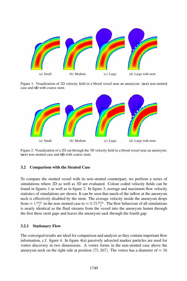
To analyse aneurysm growth and its influence on flow dynamics, we perform some basic

tests using the three stages of our synthetic aneurysm model. The velocity fields obtained

with the models are shown in figures 1 and 2. The results from all simulation models share

a parabolic velocity profile throughout the blood vessel, a drop in velocity magnitude near

the opening of the aneurysm and a significant velocity magnitude at the aneurysm neck.

The larger the aneurysm the higher the drop in magnitude in the vessel at the neck, cf.

isoline velocity plot in figure 1. Comparing the converged results no such high velocity

magnitudes do occur inside the aneurysm. On average the velocity magnitude is only

≈ 1mms

whereas in aneurysm neck the velocity is ≈ 14−20mms

depending on the scenario

used (c.f. figure 3(c)).

1748

(a) Small (b) Medium (c) Large (d) Large with stent

Figure 1: Visualization of 2D velocity field in a blood vessel near an aneurysm: (a-c) non-stentedcase and (d) with coarse stent.

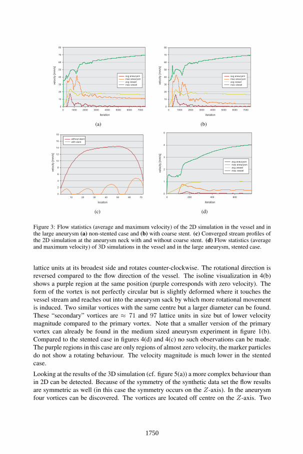
(a) Small (b) Medium (c) Large (d) Large with stent

Figure 2: Visualization of a 2D cut through the 3D velocity field in a blood vessel near an aneurysm:(a-c) non-stented case and (d) with coarse stent.

3.2 Comparison with the Stented Case

To compare the stented vessel with its non-stented counterpart, we perform a series of

simulations where 2D as well as 3D are evaluated. Colour coded velocity fields can be

found in figures 1 as well as in figure 2. In figure 3, average and maximum flow velocity

statistics of simulations are shown. It can be seen that much of the inflow at the aneurysm

neck is effectively disabled by the stent. The average velocity inside the aneurysm drops

from ≈ 1mms

in the non-stented case to ≈ 0.75mms

. The flow behaviour of all simulations

is nearly identical as the fluid streams from the vessel into the aneurysm lumen through

the first three stent gaps and leaves the aneurysm sack through the fourth gap.

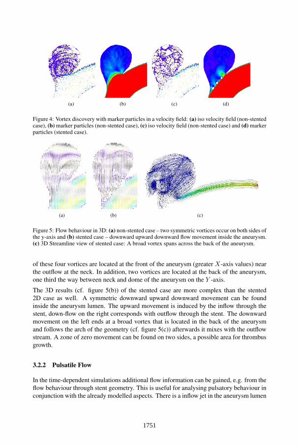
3.2.1 Stationary Flow

The converged results are ideal for comparison and analysis as they contain important flow

information, c.f. figure 4. In figure 4(a) passively advected marker particles are used for

vortex discovery in two dimensions. A vortex forms in the non-stented case above the

aneurysm neck on the right side at position (75, 267). The vortex has a diameter of ≈ 56

1749

iteration

0 1000 2000 3000 4000 5000 6000 7000

0

10

20

30

40

50

60

70

80

velo

city [m

m/s

]

avg aneurysm

max aneurysm

avg vessel

max vessel

(a)

iteration

0 1000 2000 3000 4000 5000 6000 7000

0

10

20

30

40

50

60

70

80

avg aneurysm

max aneurysm

avg vessel

max vesselve

locity [m

m/s

]

(b)

location

10 20 30 40 50 60 70

0

2

4

6

8

10

12

14

16

18

without stent

with stent

ve

locity [m

m/s

]

(c)

iteration

0 200 400 600

0

1

2

3

4

5

avg aneurysm

max aneurysm

avg vessel

max vesselve

locity [m

m/s

]

(d)

Figure 3: Flow statistics (average and maximum velocity) of the 2D simulation in the vessel and inthe large aneurysm (a) non-stented case and (b) with coarse stent. (c) Converged stream profiles ofthe 2D simulation at the aneurysm neck with and without coarse stent. (d) Flow statistics (averageand maximum velocity) of 3D simulations in the vessel and in the large aneurysm, stented case.

lattice units at its broadest side and rotates counter-clockwise. The rotational direction is

reversed compared to the flow direction of the vessel. The isoline visualization in 4(b)

shows a purple region at the same position (purple corresponds with zero velocity). The

form of the vortex is not perfectly circular but is slightly deformed where it touches the

vessel stream and reaches out into the aneurysm sack by which more rotational movement

is induced. Two similar vortices with the same centre but a larger diameter can be found.

These “secondary” vortices are ≈ 71 and 97 lattice units in size but of lower velocity

magnitude compared to the primary vortex. Note that a smaller version of the primary

vortex can already be found in the medium sized aneurysm experiment in figure 1(b).

Compared to the stented case in figures 4(d) and 4(c) no such observations can be made.

The purple regions in this case are only regions of almost zero velocity, the marker particles

do not show a rotating behaviour. The velocity magnitude is much lower in the stented

case.

Looking at the results of the 3D simulation (cf. figure 5(a)) a more complex behaviour than

in 2D can be detected. Because of the symmetry of the synthetic data set the flow results

are symmetric as well (in this case the symmetry occurs on the Z-axis). In the aneurysm

four vortices can be discovered. The vortices are located off centre on the Z-axis. Two

1750

(a) (b) (c) (d)

Figure 4: Vortex discovery with marker particles in a velocity field: (a) iso velocity field (non-stentedcase), (b) marker particles (non-stented case), (c) iso velocity field (non-stented case) and (d) markerparticles (stented case).

(a) (b) (c)

Figure 5: Flow behaviour in 3D: (a) non-stented case – two symmetric vortices occur on both sides ofthe y-axis and (b) stented case – downward upward downward flow movement inside the aneurysm.(c) 3D Streamline view of stented case: A broad vortex spans across the back of the aneurysm.

of these four vortices are located at the front of the aneurysm (greater X-axis values) near

the outflow at the neck. In addition, two vortices are located at the back of the aneurysm,

one third the way between neck and dome of the aneurysm on the Y -axis.

The 3D results (cf. figure 5(b)) of the stented case are more complex than the stented

2D case as well. A symmetric downward upward downward movement can be found

inside the aneurysm lumen. The upward movement is induced by the inflow through the

stent, down-flow on the right corresponds with outflow through the stent. The downward

movement on the left ends at a broad vortex that is located in the back of the aneurysm

and follows the arch of the geometry (cf. figure 5(c)) afterwards it mixes with the outflow

stream. A zone of zero movement can be found on two sides, a possible area for thrombus

growth.

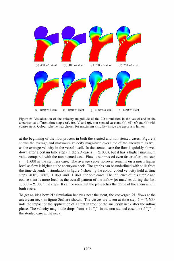
3.2.2 Pulsatile Flow

In the time-dependent simulations additional flow information can be gained, e.g. from the

flow behaviour through stent geometry. This is useful for analysing pulsatory behaviour in

conjunction with the already modelled aspects. There is a inflow jet in the aneurysm lumen

1751

(a) 400 w/o stent (b) 400 w/ stent (c) 750 w/o stent (d) 750 w/ stent

(e) 1050 w/o stent (f) 1050 w/ stent (g) 1350 w/o stent (h) 1350 w/ stent

Figure 6: Visualisation of the velocity magnitude of the 2D simulation in the vessel and in theaneurysm at different time steps: (a), (c), (e) and (g), non-stented case and (b), (d), (f) and (h) withcoarse stent. Colour scheme was chosen for maximum visibility inside the aneurysm lumen.

at the beginning of the flow process in both the stented and non-stented cases. Figure 3

shows the average and maximum velocity magnitude over time of the aneurysm as well

as the average velocity in the vessel itself. In the stented case the flow is quickly slowed

down after a certain time step (in the 2D case t = 2, 000), but it has a higher maximum

value compared with the non-stented case. Flow is suppressed even faster after time step

t = 1, 600 in the stentless case. The average curve however remains on a much higher

level as flow is higher at the aneurysm neck. The graphs can be underlined with stills from

the time-dependent simulation in figure 6 showing the colour coded velocity field at time

steps ”400”, ”750”, ”1, 050” and ”1, 350” for both cases. The influence of this simple and

coarse stent is more local as the overall pattern of the inflow jet matches during the first

1, 600− 2, 000 time steps. It can be seen that the jet reaches the dome of the aneurysm in

both cases.

To get an idea how 2D simulation behaves near the stent, the converged 2D flows at the

aneurysm neck in figure 3(c) are shown. The curves are taken at time step t = 7, 500,

note the impact of the application of a stent in front of the aneurysm neck after the inflow

phase. The velocity magnitude drops from ≈ 14mms

in the non-stented case to ≈ 5mms

in

the stented case at the neck.

1752

3.3 Execution times

A straight forward OpenMP x86 implementation on a 2.93 Ghz intel Core i7 processor

is outperformed by a factor of 130 − 200 with our OpenCL implementation on a nVidia

GTX 560 Ti. With the above data sets 1225 and 84 frames per second can be reached in

2D repectively 3D. This perfomance gain is largely influenced by memory performance.

4 Discussion

The construct of mathematical representation of patient-specific anatomy is both feasible

and applicable. A variety of practical issues has to be considered towards establishment of

mathematical model-based tailor-made aneurysm therapy to realize personalized stenting

for individual patients based on clinical and radiological findings.

In order to gain insights in the time-dependent flow process during a cardiac cycle LBM

has proven to be a viable solution. The key conclusion is that the inflow phase into the

aneurysm lumen during a cardiac cycle seems to be most interesting to analyse. The ques-

tion of what influence do far reaching and concentrated inflow jets have on the integrity of

the aneurysm sack has not been finally answered although some investigations have tried

to [CMWP11]. The growth of aneurysms in conjunction with CFD has not been studied

to date. Because of the runtime efficiency of the LBM, it seems possible to gain further

insight in the complex flow processes of real geometry. A full 3D simulation is needed as

indicated by the more complex results even in the simple synthetic case. The interactive

frame rates of parallel LBM simulations can provide key simulation constellations.

The developed method has to be refined in a way that it provides the necessary resolution,

respects pulsatory and material behaviour and models thrombosation to automatically find

a stent geometry that is best for a specific situation. Further investigations are needed.

References

[AML+09] S. Appanaboynia, F. Mut, R. Löhner, C. Putman, and J. Cebral. Simulation of intracra-nial aneurysm stenting: techniques and challenges. Comput. Methods Appl. Mech.Engrg., 198:3567–3582, 2009.

[Cha06] H.S. Chang. Simulation of the natural history of cerebral aneurysms based on datafrom the International Study of Unruptured Intracranial Aneurysms. J Neurosurg,104(2):188–94, 2006.

[CMWP11] J. R. Cebral, F. Mut, J. Weir, and C. M. Putman. Association of hemodynamic char-acteristics and cerebral aneurysm rupture. AJNR Am J Neuroradiol, 32(2):264–270,2011.

[CSV11] A. Chien, J. Sayre, and F. Vintildeuela. Comparative Morphological Analysis of theGeometry of Ruptured and Unruptured Aneurysms. Neurosurgery, 69(2):349–356,2011.

1753

[GJMS11] A. Gambaruto, J. Janela, A. Moura, and A. Sequeira. Sensitivity of hemodynamics ina patient specific cerebral aneurysm to vascular geometry and blood rheology. MathBiosci Eng, 8(2):409–423, 2011.

[IOTK04] T. Inamuro, T. Ogata, S. Tajima, and N. Konishi. A lattice Boltzmann method for in-compressible two-phase flows with large density differences. Journal of ComputationalPhysics, 198(2):628–644, 2004.

[JLN+09] S.W. Joo, S. Lee, S.J. Noh, Y.G. Jeong, M.S. Kim, and Y.T. Jeong. What Is the Signif-icance of a Large Number of Ruptured Aneurysms Smaller than 7 mm in Diameter? JKorean Neurosurg Soc, 45(2):85–89, 2009.

[JY03] M. Junk and W.-A. Yong. Rigorous Navier-Stokes Limit of the Lattice BoltzmannEquation. Asymptotic Analysis, 35:165–184, 2003.

[KTTM08] M. Kim, D.B. Taulbee, M. Tremmel, and H. Meng. Comparison of two stents in mod-ifying cerebral aneurysm hemodynamics. Ann Biomed Eng, 36:726–741, 2008.

[KYGB11] M. Kamran, J. Yarnold, I.Q. Grunwald, and J.V. Byrne. Assessment of angiographicoutcomes after flow diversion treatment of intracranial aneurysms: a new gradingschema. Neuroradiology, 53(7):501–508, 2011.

[LLW+11] J. Lu, J. Liu, L. Wang, P. Qi, and D. Wang. Tiny intracranial aneurysms: Endovasculartreatment by coil embolisation or sole stent deployment. Eur J Radiol, 2011.

[MKS+02] A. Molyneux, R. Kerr, I. Stratton, P. Sandercock, M. Clarke, J. Shrimpton, and R. Hol-man. International Subarachnoid Aneurysm Trial (ISAT) of neurosurgical clippingversus endovascular coiling in 2143 patients with ruptured intracranial aneurysms: arandomised trial. Lancet, 360(9342):1267–1274, 2002.

[MKS+10] A. Morita, T. Kimura, M. Shojima, T. Sameshima, and T. Nishihara. Unruptured in-tracranial aneurysms: current perspectives on the origin and natural course, and questfor standards in the management strategy. Neurol Med Chir (Tokyo), 50(9):777–87,2010.

[OMH+08] T. Ohshima, S. Miyachi, K.-I. Hattori, I. Takahashi, K. Ishii, T. Izumi, and J. Yoshida.Risk of aneurysmal rupture: the importance of neck orifice positioning-assessment us-ing computational flow simulation. Neurosurgery, 62(4):767–773, 2008.

[Rin08] G.J.E. Rinkel. Natural history, epidemiology and screening of unruptured intracranialaneurysms. J Neuroradiol, 35(2):99–103, 2008.

[SC93] X. Shan and H. Chen. Lattice Boltzmann model for simulating flows with multiplephases and components. Phys. Rev. E, 47(3):1815–1819, Mar 1993.

[ST06] M.C. Sukop and D.T. Thorne. Lattice Boltzmann Modeling: An Introduction for Geo-scientists and Engineers. Springer, Heidelberg, Berlin, New York, 2006.

[Suc01] S. Succi. The lattice Boltzmann equation for fluid dynamics and beyond. ClarendonPress Oxford University Press, Oxford New York, 2001.

[Yos06] Y. Yoshimoto. A mathematical model of the natural history of intracranial aneurysms:quantification of the benefit of prophylactic treatment. J Neurosurg, 104(2):195–200,2006.

[YS06] P. Yuan and L. Schaefer. Equations of state in a lattice Boltzmann model. Physics ofFluids, 18, 2006.

[ZH95] Q. Zou and X. He. On pressure and velocity flow boundary conditions for the latticeBoltzmann BGK model. Biophysics, 9:16, 1995.

1754