79
Exponential Families & From Prior Information to Prior Distribution Timo Koski 20.01.2010 Timo Koski () Matematisk statistik 20.01.2010 1 / 78

Exponential Families & From Prior Information to PriorDistribution
Timo Koski
20.01.2010
Timo Koski () Matematisk statistik 20.01.2010 1 / 78
These notes
The material in these notes was intially based on
C.P. Roberts: Bayesian Choice, Second Edition, Springer-Verlag,Berlin , 2001.
Some auxuliary results required are quoted from
M.J. Schervish: Theory of Statistics , Springer-Verlag, Berlin , 1995.
An idiosyncracy of Roberts is that u · x may designate both the product ofreal numbers u and x as well as the scalar product of vectors u and x .Otherwise an effort has been made to unify the notation with the notes byHenrik. In addition, Roberts prefers to write x for both outcome andrandom variable.
Timo Koski () Matematisk statistik 20.01.2010 2 / 78

Notation
An idiosyncracy of Roberts is that u · x may designate both the product ofreal numbers u and x as well as the scalar product of vectors u and x . Inaddition, Roberts prefers to write x for both outcome and random variable.Roberts deals with the natural exponential family to be introduced below.Otherwise an effort has been made to accomodate to the notation withthe notes by Henrik.
Timo Koski () Matematisk statistik 20.01.2010 3 / 78

Parametric statistical model recalled
x is an observation of a random variable X , x ∈ X (=sample space).
x ∼ fX |Θ (x |θ)
fX |Θ (x |θ) is a probability density w.r.t. to a σ finite measure ν on X .fX |Θ (x |θ) is a known function of x and θ.θ is an unknown parameter ∈ Ω ⊆ a vector space of finite dimension.
Timo Koski () Matematisk statistik 20.01.2010 4 / 78

Exponential Families
The family of distributions µX |Θ with densities w.r.t. to a σ-finite measureν on X defined by
dµX |Θ=θ
dν(x | θ) = fX |Θ (x |θ) = C (θ)h(x)eR(θ)·T (x)
is called an exponential family (of dimension k), where
C (θ) and h(x) are measurable functions from Ω and X to R+,
R(θ) and T (x) are measurable functions from Ω and X to Rk ,
R(θ) · T (x) is a scalar product in Rk , i.e.,
R(θ) · T (x) =k
∑i=1
Ri (θ) · Ti (x)
Timo Koski () Matematisk statistik 20.01.2010 5 / 78

Exponential Families
The family of distributions µX |Θ has densities w.r.t. to a σ-finitemeasure ν on X , if for all θ ∈ Ω, µX |Θ=θ << ν. If there is anotherσ-finite measure, say ν, such that for all θ, µX |Θ=θ << ν,, then thereexists a representation as above. The dimension k may depend on thedominating measure.
If θ0 ∈Ω, then µX |Θ=θ << µX |Θ=θ0and the density of µX |Θ=θ w.r.t.
µX |Θ=θ0on X is
dµX |Θ=θ
dµX |Θ=θ0
(x | θ) =C (θ)
C (θ0)e(R(θ)−R(θ0))·T (x)
Hence, e.g., the family U (0, θ) , θ ∈ Ω = (0, ∞) cannot be anexponential family.
Timo Koski () Matematisk statistik 20.01.2010 6 / 78

EXAMPLES OF EXPONENTIAL FAMILIES: Be(θ)
Ω = (0, 1), ν is the counting measure1.
fX |Θ (x |θ) = θx · (1− θ)1−x . x = 0, 1
We writefX |Θ (x |θ) = C (θ)eR(θ)·x ,
where
C (θ) = e log 1−θ, T (x) = x , R(θ) = logθ
1− θ, h(x) = 1.
1X= positive integers, ν(A) = the number of elements in A ⊂ XTimo Koski () Matematisk statistik 20.01.2010 7 / 78

EXAMPLES OF EXPONENTIAL FAMILIES: N(µ, σ2)
x (n) = (x1, x2, . . . , xn), xi I.I.D. ∼ N(µ, σ2).
f (x (n)|µ, σ2) =1
σn (2π)n/2e− 1
2σ2 ∑ni=1(xi−µ)2
=1
(2π)n/2σ−ne
− nµ2
2σ2 e− 1
2σ2 ∑ni=1 x2
i +µ
σ2 nx .
Timo Koski () Matematisk statistik 20.01.2010 8 / 78

EXAMPLES OF EXPONENTIAL FAMILIES: N(µ, σ2)
Ω = R × (0, ∞), ν = Lebesgue measure on Rn. ,
f (x (n)|µ, σ2) =1
(2π)n/2σ−ne
− nµ2
2σ2 e− 1
2σ2 ∑ni=1 x2
i +µ
σ2 nx .
C (θ) = σ−ne− nµ2
2σ2 , h(x) =1
(2π)n/2.
R(θ) · T(
x (n))
= R1(θ)T1
(
x (n))
+ R2(θ)T2
(
x (n))
T1
(
x (n))
=n
∑i=1
x2i , T2
(
x (n))
= nx
R1(θ) = − 1
2σ2, R2(θ) =
µ
σ2
Timo Koski () Matematisk statistik 20.01.2010 9 / 78

SOME COMMON EXPONENTIAL FAMILIES
Poisson Po(θ), Gamma Ga(p, θ), Binomial Bin(n, θ), Negative BinomialNeg(m, θ), Multinomial, Inverse Gaussian, Weibull (with known shapeparameter)
Timo Koski () Matematisk statistik 20.01.2010 10 / 78

Inverse Gaussian
µ > 0, λ > 0, 0 < x < ∞, θ = (µ, λ)
f (x | µ, λ) =
[
λ
2πx3
]1/2
exp−λ(x − µ)2
2µ2x
The inverse Gaussian distribution is a two-parameter exponential familywith natural parameters −λ/(2µ2) and −λ/2, and T1(X ) = X andT2(X ) = 1/X .
Timo Koski () Matematisk statistik 20.01.2010 11 / 78

Natural Parameter, Natural parameter space
Clearly the density
fX |Θ (x | θ) = C (θ)h(x)eR(θ)·T (x)
depends only onR = (R1(θ), R2(θ), . . . , Rk(θ)) .
We call R the natural parameter.
N = N (ν) :=
R ∈ Rk |∫
Xh(x)eR ·T (x)ν(dx) < ∞
N is called the natural parameter space, we assume that N = Ω.
Timo Koski () Matematisk statistik 20.01.2010 12 / 78

Density of T
From Schervish p. 103:
Lemma
If X has an exponential family distribution, then T (X ) has an exponential
family distribution, and there exists a measure νT such that
dµT |ΘdνT
(t) = C (θ)et·θ
This will be discussed further in the lecture on sufficient statistics. A proofis found on p. 17 in notes by Henrik.
Timo Koski () Matematisk statistik 20.01.2010 13 / 78
Natural Exponential Families (1)
Thus, Θ ⊆ Rk and X ⊆ Rk , we can make a change of variable & relabel:R(θ) ↔ θ and T (x) ↔ x .
fX |Θ (x | θ) = C (θ)h(x)eθ·x
and the family is said to be a natural exponential family . Here θ · x isinner product on Rk .
Timo Koski () Matematisk statistik 20.01.2010 14 / 78

Exponential Families: the natural parameter space
Thus
1 = C (θ)
∫
Xh(x)eθ·x ν(dx).
C (θ) =1
∫
X h(x)eθ·x ν(dx).
N (ν) :=
θ ∈ Rk |∫
Xh(x)eθ·x ν(dx) < ∞
N = N (ν) is called the natural parameter space, possibly 6= Ω.
Timo Koski () Matematisk statistik 20.01.2010 15 / 78

The natural parameter space
N :=
θ|∫
Xh(x)eθ·x ν(dx) < ∞
An application of convexity of exp(·) yields that N is convex (asshown below).
WE ASSUME that N is an open set in Rk . Then we are dealing witha regular exponential family2
2O. Barndorff-Nielsen: Information and Exponential families in Statistical Theory, J.Wiley, 1978
Timo Koski () Matematisk statistik 20.01.2010 16 / 78
Natural Exponential Families (2)
Sats1
C (θ) is a convex function.
Proof: θ1 and θ2 are two points in N and 0 ≤ λ ≤ 1. Then, since theexponential function is convex,
1
C (λθ1 + (1 − λ)θ2)=
∫
Xh(x)e(λθ1+(1−λ)θ2)·xν(dx)
≤∫
Xh(x)
(
λeθ1 ·x + (1 − λ)eθ2 ·x)
ν(dx) = λ1
C (θ1)+ (1 − λ)
1
C (θ2).
Timo Koski () Matematisk statistik 20.01.2010 17 / 78

Natural Exponential Families (3)
Foljdsats
N is a convex set.
Proof: θ1 and θ2 are two points in N and 0 ≤ λ ≤ 1. Then 1C (θ1)
< ∞
and 1C (θ2)
< ∞, and since 1C (θ) is convex, we get that
λθ1 + (1− λ)θ2 ∈ N .
Timo Koski () Matematisk statistik 20.01.2010 18 / 78

Natural Exponential Families (4)
fX |Θ (x | θ) = h(x)eθ·x−ψ(θ)
whereψ (θ) = − log C (θ).
The function ψ (θ) is called the cumulant function.
Timo Koski () Matematisk statistik 20.01.2010 19 / 78

Natural Exponential Families (5)
Proposition
The moment generating function of a natural exponential family is
M(u) = Eθ
[
euX]
=C (θ)
C (θ + u)
Proof:
Eθ
[
euX]
=
∫
Xeux fX |Θ (x | θ) ν(dx) =
∫
Xeuxh(x)eθ·x−ψ(θ)ν(dx)
= e−ψ(θ)
∫
Xh(x)e(u+θ)·xν(dx) =
C (θ)
C (θ + u).
Timo Koski () Matematisk statistik 20.01.2010 20 / 78

Natural Exponential Families: Poisson Distribution
f (x | λ) = e−λ λx
x !, x = 0, 1, 2, . . . ,
f (x | λ) =1
x !eθx−eθ
ψ (θ) = eθ , θ = log λ, h(x) =1
x !
Moment generating function: M(u) = C (θ)C (θ+u) ,
C (θ) = e−ψ(θ) = e−eθ= e−λ, C (θ + u) = e−ψ(θ+u) = e−λeu
I.e., M(u) = e−λeλeu= eλ(eu−1)
Timo Koski () Matematisk statistik 20.01.2010 21 / 78

Timo Koski () Matematisk statistik 20.01.2010 22 / 78

Mean in a Natural Exponential Family
If Eθ [X ] denotes the mean (vector) of X ∼ fX |Θ (x |θ) in a natural family,then3
Eθ [X ] =
∫
Xxf (x | θ) dx = ∇θψ (θ) .
where θ ∈ int(N ) and X ⊆ Rk .Proof:
∫
Xxf (x | θ) dx = e−ψ(θ)
∫
Xh(x)xeθ·xdx .
3∇θψ (θ) =(
∂∂θ1
ψ (θ) , ∂∂θ2
ψ (θ) , . . . , ∂∂θk
ψ (θ))T
Timo Koski () Matematisk statistik 20.01.2010 22 / 78

Mean in a Natural Exponential Family
e−ψ(θ)
∫
Xh(x)xeθ·xdx = e−ψ(θ)
∫
Xh(x)∇θe
θ·xdx
= 4e−ψ(θ)∇θ
∫
Xh(x)eθ·xdx = e−ψ(θ)∇θ
1
C (θ)=
= e−ψ(θ) (−∇θC (θ))
C (θ)2
= C (θ)(−∇θC (θ))
C (θ)2=
(−∇θC (θ))
C (θ)
= ∇θ(− log C (θ)) = ∇θψ (θ) .
4It is permissible to interchange integration and derivation, Schervish Thm 2.64. p.105
Timo Koski () Matematisk statistik 20.01.2010 23 / 78

Mean in a Natural Exponential Family : PoissonDistribution
f (x | λ) =1
x !eθx−eθ
ψ (θ) = eθ
Eθ [X ] =d
dθψ (θ) = eθ = λ.
Timo Koski () Matematisk statistik 20.01.2010 24 / 78

Uncertainty
Uncertainty about the unknown θ is modeled by a probability distributionπ (θ), and πΘ|X (θ|x) expresses the uncertainty about the unknown θafter the observation of x .We use probability as tool for all parts of our analysis. This is coherence.Mathematically: the unknown θ becomes an outcome of a randomvariable, i.e., (X , Θ) will have a joint distribution. For the preciseformulation of this see the notes by Henrik.
Timo Koski () Matematisk statistik 20.01.2010 25 / 78

Bayesian Parametric Statistical Model
A Bayesian parametric statistical model consists of
a parametric modelx ∼ fX |Θ (x |θ)
a prior density (an improper density can be used)
θ ∼ π(θ)
The quantity of interest: posterior distribution
θ|x ∼ πΘ|X (θ|x) ∝ fX |Θ (x |θ) · π(θ)
Timo Koski () Matematisk statistik 20.01.2010 26 / 78

Bayes’ rule: parametric model
πΘ|X (θ|x) =fX |Θ (x | θ) · π (θ)
∫
ΘfX |Θ (x | θ) · π (θ) dθ
,
Terminology for Bayes’ Rule:
π (θ) : prior density on Ω; here w.r.t. the Lebesgue measure.
πΘ|X (θ|x) : posterior density on Ω, here w.r.t. the Lebesguemeasure.
m(x) =∫
ΘfX |Θ (x | θ) · π (θ) dθ : marginal distribution of x , also
known as the prior predictive distribution of x .
Timo Koski () Matematisk statistik 20.01.2010 27 / 78

Q: How do we choose π (θ) ?
Assessment (by Questionnaries)
Conjugate prior
Non-informative prior
Laplace’s priorJeffreys’ prior
Maximum entropy prior
Timo Koski () Matematisk statistik 20.01.2010 28 / 78

Assessment of prior knowledge
(One form of) Bayesian statistics relies upon a personalistic theory of
probability for quantification of prior knowledge. In such a theory
probability measures the confidence that a particular individual (assessor)has in the truth of a particular proposition
no attempt is made to specify which assessments are correct
personal probabilities should satisfy certain postulates of coherence.
Timo Koski () Matematisk statistik 20.01.2010 29 / 78

R.L.Winkler in
Robert L. Winkler: The Assessment of Prior Distributions in BayesianAnalysisJournal of the American Statistical Association, Vol. 62, No. 319. (Sep.,1967), pp. 776-800.)
devises questionnaires (or interviews) to elicit information to write down a prior
distribution. Students of Univ. of Chigago were asked to, e.g., assess the
uncertainty about the probability of a randomly chosen student of Univ. of
Chigago being Roman Catholic using a probability distribution. The assessment
was done by four different methods, like giving fractiles, making bets, assessing
impact of additional data, drawing graphs. One interesting finding is that the
assessments by the same person using different methods may be conflicting.
Timo Koski () Matematisk statistik 20.01.2010 30 / 78

Diffuse/Non-diffuse prior distributions by assessment
The priors in Winkler’s study are not diffuse: the students of Univ. ofChigago have, since they have been around, an idea about the number ofRoman Catholics at the campus of of Univ. of Chigago.
Timo Koski () Matematisk statistik 20.01.2010 31 / 78

Choice of prior distributions by assessment: Elicitingprobabilities
R.L. Keeney & D. von Winterfeldt: Eliciting Probabilities fromExperts in Complex Technical Problems. IEEE Transactions on
Engineering Management, Vol. 38, 1991, pp.191−201.
K.M. Chaloner & G.T. Duncan: Assessment of a Beta Distribution:PM Elicitation. The Statistician, 32, 1983, pp. 174−180
One more point ⇒
Timo Koski () Matematisk statistik 20.01.2010 32 / 78
Assessing Priors: Conjugate Prior
The interviews of Winkler were mathematically speaking all concerned with
assessing the prior of θ in a Bernoulli Be (θ) − I.I.D. process. Winkler claims a
sensitivity analysis (loc.cit p. 791) showing that the prior distributions assessed by
the interviews yielded posterior distributions that were ‘only little’ different (by a
test of goodness-of-fit) from those obtained from Beta densities on θ. Beta
densities are conjugate priors.
An intuitive way of understanding conjugate priors is that with conjugatepriors the prior knowledge can be translated into equivalent sampleinformation. A formal definition of conjugate priors follows.
Timo Koski () Matematisk statistik 20.01.2010 33 / 78

Conjugate Prior
Definition
Let F be a class of probability densities fX |Θ (x | θ). A family of
probability distributions Π on Θ is said to be conjugate or closed under
sampling for F , if for every prior π ∈ Π, the posterior distribution
πΘ|X (θ|x) also belongs to Π for every f ∈ F .
Timo Koski () Matematisk statistik 20.01.2010 34 / 78

Conjugate Family of Priors
A conjugate family is usually associated with a particular samplingdistribution that is even characteristic of conjugate priors: exponentialfamilies.
Timo Koski () Matematisk statistik 20.01.2010 35 / 78
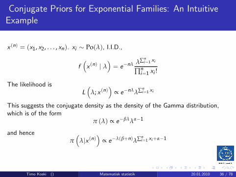
Conjugate Priors for Exponential Families: An IntuitiveExample
x (n) = (x1, x2, . . . , xn). xi ∼ Po(λ), I.I.D.,
f(
x (n) | λ)
= e−nλ λ∑ni=1 xi
∏ni=1 xi !
The likelihood isL(
λ; x (n))
∝ e−nλλ∑ni=1 xi
This suggests the conjugate density as the density of the Gamma distribution,which is of the form
π (λ) ∝ e−βλλα−1
and henceπ(
λ|x (n))
∝ e−λ(β+n)λ∑ni=1 xi+α−1
Timo Koski () Matematisk statistik 20.01.2010 36 / 78

Conjugate Family of Priors for Exponential Families
Proposition
For the natural exponential family
fX |Θ (x | θ) = h(x)eθ·x−ψ(θ)
the conjugate familya is given by
π (θ) = ψ (θ|µ, λ) = K (µ, λ) eθ·µ−λψ(θ)
and the posterior is
ψ (θ|µ + x , λ + 1) .
a(if this is a probabilty density, c.f. below)
Timo Koski () Matematisk statistik 20.01.2010 37 / 78

Conjugate Priors for Exponential Families: Proof
Proof: By Bayes’ rule
π (θ|x) =f (x | θ) π (θ)
m(x)
We havef (x | θ) π (θ) = h(x)eθ·x−ψ(θ)ψ (θ|µ, λ)
= h(x)K (µ, λ) eθ·(x+µ)−(1+λ)ψ(θ)
Timo Koski () Matematisk statistik 20.01.2010 38 / 78

Conjugate Priors for Exponential Families: Proof
m(x) =
∫
Θ
f (x | θ) π (θ) dθ =
= h(x)K (µ, λ)
∫
Θ
eθ·(x+µ)−(1+λ)ψ(θ)dθ
= h(x)K (µ, λ) K (x + µ, λ + 1)−1 .
Timo Koski () Matematisk statistik 20.01.2010 39 / 78
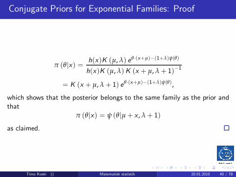
Conjugate Priors for Exponential Families: Proof
π (θ|x) =h(x)K (µ, λ) eθ·(x+µ)−(1+λ)ψ(θ)
h(x)K (µ, λ) K (x + µ, λ + 1)−1
= K (x + µ, λ + 1) eθ·(x+µ)−(1+λ)ψ(θ),
which shows that the posterior belongs to the same family as the prior andthat
π (θ|x) = ψ (θ|µ + x , λ + 1)
as claimed.
Timo Koski () Matematisk statistik 20.01.2010 40 / 78

Conjugate Priors for Exponential Families
If λ > 0 andµλ ∈ Int(N ), then
π (θ) = ψ (θ|µ, λ) = K (µ, λ) eθ·µ−λψ(θ)
is a probability density on Θ (proof is an exercise for the reader), which ispresupposed in the proof above.The parameters of the prior, λ and µ, are called hyperparameters.
Timo Koski () Matematisk statistik 20.01.2010 41 / 78

Mean for Exponential Families
We have the following properties:
if π (θ) = K (xo , λ) eθ·xo−λψ(θ) then
ξ(θ) =
∫
Θ
Eθ [x ] π (θ) dθ =xo
λ
This has been proved by Diaconis and Ylvisaker5. The proof is notsummarized here.
5P. Diaconis & D. Ylvisaker: Conjugate Priors for Expoenntial Families. The Annals
of Statistics, vol. 7, 1979, pp. 269−281.Timo Koski () Matematisk statistik 20.01.2010 42 / 78

Posterior Means with Conjugate Priors for ExponentialFamilies
if π (θ) = K (µ, λ) eθ·µ−λψ(θ) then
∫
Θ
Eθ [x ] π(
θ|x (n))
dθ =µ + nx
λ + n
This follows from the preceding, as shown by Diaconis and Ylvisaker(1979). In fact Diaconis and Ylvisaker prove that this is a characterizationof conjugate priors for regular exponential families.
Timo Koski () Matematisk statistik 20.01.2010 43 / 78
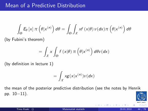
Mean of a Predictive Distribution
∫
Θ
Eθ [x ] π(
θ|x (n))
dθ =
∫
Θ
∫
Xxf (x |θ) ν(dx)π
(
θ|x (n))
dθ
(by Fubini’s theorem)
=
∫
Xx
∫
Θ
f (x |θ) π(
θ|x (n))
dθν(dx)
(by definition in lecture 1)
=
∫
Xxg(x |x (n))ν(dx)
the mean of the posterior predictive distribution (see the notes by Henrikpp. 10−11).
Timo Koski () Matematisk statistik 20.01.2010 44 / 78

Mean of a Predictive Distribution
Hence if conjugate priors for exponential families are used, then
∫
Xxg(x |x (n))ν(dx) =
µ + nx
λ + n
is the mean of the corresponding predictive distribution. This suggests µand λ as ’virtual observations’.
Timo Koski () Matematisk statistik 20.01.2010 45 / 78

Laplace’s Prior
P.S. Laplace6 formulated the principle of insufficient reason to choose aprior as a uniform prior. There are drawbacks in this. Consider Laplace’sprior for θ ∈ [0, 1]
π (θ) =
1 0 ≤ θ ≤ 10 elsewhere,
Then considerφ = θ2.
6http://www-groups.dcs.st-and.ac.uk/∼history/Mathematicians/Laplace.html
Timo Koski () Matematisk statistik 20.01.2010 46 / 78

Laplace’s Prior
We find the density of φ = θ2. Take 0 < v < 1.
Fφ(v ) = P (φ ≤ v ) = P(
θ ≤√
v)
=
∫
√v
0π (θ) dθ
=√
v .
fφ(v ) =d
dvFφ(v ) =
d
dv
√v =
1
2
1√v
which is no longer uniform. But how come we should have non-uniformprior density for θ2 when there is full ignorance about θ ?
Timo Koski () Matematisk statistik 20.01.2010 47 / 78

Invariant Prior
We want to use a method (M) for choosing a prior density with the followingproperty:If ψ = g (θ), g a monotone map, we have used the method (M) to find π, thenthe density of ψ given by the method (M) is
πΨ(ψ) = π(
g−1(ψ))
· | d
dψg−1 (ψ) |,
which is the standard probability calculus rule for change of variable in a
probability density.
Timo Koski () Matematisk statistik 20.01.2010 48 / 78

Invariant Prior: Jeffreys’ Prior
We shall now describe one method (M), i.e., Jeffreys’ prior.In order to introduce Jeffreys’ prior we need first to define Fisherinformation, which will be needed even for purposes other than choice ofprior.
Timo Koski () Matematisk statistik 20.01.2010 49 / 78

Fisher Information of X
A parametric model x ∼ f (x |θ), where f (x |θ) is differentiable w.r.t toθ ∈ R , we define I (θ), Fisher information of x , as
I (θ) =
∫
X
(
∂ log f (x |θ)
∂θ
)2
f (x |θ) ν(dx)
Conditions for existence of I (θ) are given in Schervish (1995), p. 111.
Timo Koski () Matematisk statistik 20.01.2010 50 / 78
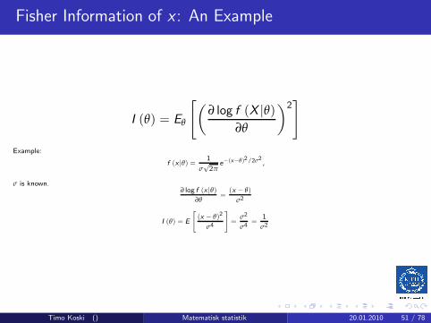
Fisher Information of x : An Example
I (θ) = Eθ
[
(
∂ log f (X |θ)
∂θ
)2]
Example:
f (x |θ) =1
σ√
2πe−(x−θ)2/2σ2
,
σ is known.∂ log f (x |θ)
∂θ=
(x − θ)
σ2
I (θ) = E
[
(x − θ)2
σ4
]
=σ2
σ4=
1
σ2
Timo Koski () Matematisk statistik 20.01.2010 51 / 78

Fisher Information of x , θ ∈ Rk
x ∼ f (x |θ), where f (x |θ) is differentiable w.r.t to θ ∈ Rk , we defineI (θ), Fisher information of x , as the matrix
I (θ) = (Iij (θ))k,ki ,j=1
Iij (θ) = Covθ
(
∂ log f (x |θ)
∂θi,
∂ log f (x |θ)
∂θj
)
Timo Koski () Matematisk statistik 20.01.2010 52 / 78
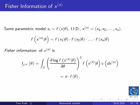
Fisher Information of x(n)
Same parametric model xi ∼ f (x |θ), I.I.D., x (n) = (x1, x2, . . . , xn).
f(
x (n)|θ)
= f (x1|θ) · f (x2|θ) · . . . · f (xn|θ)
Fisher information of x (n) is
Ix (n) (θ) =
∫
X
(
∂ log f(
x (n)|θ)
∂θ
)2
f(
x (n)|θ)
ν(
dx (n))
= n · I (θ) .
Timo Koski () Matematisk statistik 20.01.2010 53 / 78

Fisher Information of x : another form
A parametric model x ∼ f (x |θ), where f (x |θ) is twice differentiable w.r.tto θ ∈ R . If we can write
d
dθ
∫
X
(
∂ log f (x |θ)
∂θ
)
f (x |θ) ν(dx) =
=
∫
X
∂
∂θ
(
∂ log f (x |θ)
∂θ
)
f (x |θ) ν(dx),
then
I (θ) = −∫
X
(
∂2 log f (x |θ)
∂θ2
)
f (x |θ) ν(dx)
Timo Koski () Matematisk statistik 20.01.2010 54 / 78
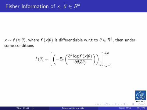
Fisher Information of x , θ ∈ Rk
x ∼ f (x |θ), where f (x |θ) is differentiable w.r.t to θ ∈ Rk , then undersome conditions
I (θ) =
[
(
−Eθ
(
∂2 log f (x |θ)
∂θi ∂θj
))
ij
]k,k
i ,j=1
Timo Koski () Matematisk statistik 20.01.2010 55 / 78

Fisher Information of x : Natural Exponential Family
For a natural exponential family
f (x | θ) = h(x)eθ·x−ψ(θ)
∂2 log f (x |θ)
∂θi ∂θj= −∂2ψ (θ)
∂θi ∂θj
so no expectation needs to be computed to obtain I (θ).
Timo Koski () Matematisk statistik 20.01.2010 56 / 78
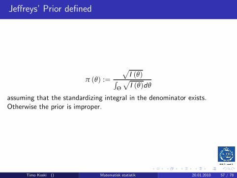
Jeffreys’ Prior defined
π (θ) :=
√
I (θ)∫
Θ
√
I (θ)dθ
assuming that the standardizing integral in the denominator exists.Otherwise the prior is improper.
Timo Koski () Matematisk statistik 20.01.2010 57 / 78
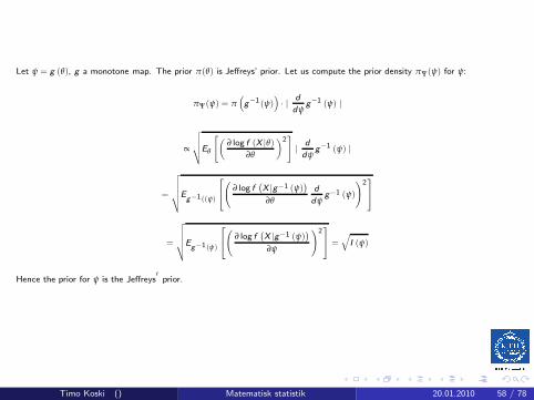
Let ψ = g (θ), g a monotone map. The prior π(θ) is Jeffreys’ prior. Let us compute the prior density πΨ(ψ) for ψ:
πΨ(ψ) = π(
g−1 (ψ))
· | d
dψg−1 (ψ) |
∝
√
√
√
√Eθ
[
(
∂ log f (X |θ)
∂θ
)2]
| d
dψg−1 (ψ) |
=
√
√
√
√
√Eg−1((ψ)
(
∂ log f(
X |g−1 (ψ))
∂θ
d
dψg−1 (ψ)
)2
=
√
√
√
√
√Eg−1(ψ)
(
∂ log f(
X |g−1 (ψ))
∂ψ
)2
=√
I (ψ)
Hence the prior for ψ is the Jeffreys′
prior.
Timo Koski () Matematisk statistik 20.01.2010 58 / 78

F = Binomial Distribution & Π =Conjugate Priors
We let Θ be a random variable, whose values are denoted by θ,Ω = (0, 1). We condition on Θ = θ, and consider X , which is the sum ofn I.I.D Be(θ) R.V’s. Hence for x = 0, 1, 2, . . . , n,
f (x |θ) = P (X = x | Θ = θ)
=
(
n
x
)
θx · (1 − θ)n−x ,
(the Binomial distribution)
Timo Koski () Matematisk statistik 20.01.2010 59 / 78

Prior Density
Any function π(·) such that
π (θ) ≥ 0, 0 ≤ θ ≤ 1,
π (θ) = 0 elsewhere,
and∫ 1
0π (θ) dθ = 1,
can serve as prior distribution.
Timo Koski () Matematisk statistik 20.01.2010 60 / 78

Improper Prior Densities
Functions with the properties
π (θ) ≥ 0, 0 ≤ θ ≤ 1,
π (θ) = 0 elsewhere,
and∫ 1
0π (θ) dθ = ∞,
are also invoked as prior distributions, and are called improper priors.
Timo Koski () Matematisk statistik 20.01.2010 61 / 78

The Posterior Density
Bayes’ rule
π (θ | x) =f (x | θ) · π (θ)
∫ 10 f (x | θ) · π (θ) dθ
, 0 ≤ θ ≤ 1
and zero elsewhere. The marginal distribution of x is
m(x) =
∫ 1
0f (x | θ) · π (θ) dθ.
Timo Koski () Matematisk statistik 20.01.2010 62 / 78

The Posterior Density
Take θ ∼ U(0, 1). i.e.,
π (θ) =
1 0 ≤ θ ≤ 10 elsewhere,
Timo Koski () Matematisk statistik 20.01.2010 63 / 78
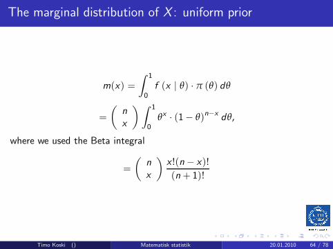
The marginal distribution of X : uniform prior
m(x) =
∫ 1
0f (x | θ) · π (θ) dθ
=
(
n
x
)∫ 1
0θx · (1− θ)n−x
dθ,
where we used the Beta integral
=
(
n
x
)
x !(n − x)!
(n + 1)!
Timo Koski () Matematisk statistik 20.01.2010 64 / 78

The Beta Density
π(θ) =
Γ(α+β)Γ(α)Γ(β)θα−1(1− θ)β−1 0 < θ < 1
0 elsewhere.
is a probability density Be(α, β).
∫ 1
0π(θ)dθ = 1 ⇔
∫ 1
0θα−1(1 − θ)β−1dp =
Γ(α)Γ(β)
Γ(α + β).
Timo Koski () Matematisk statistik 20.01.2010 65 / 78

The Beta Integral
∫ 1
0θα−1(1 − θ)β−1dp =
Γ(α)Γ(β)
Γ(α + β).
Recall also that Γ(x + 1) = x !, if x is a positive integer. α = β = 1 givesthe distribution U(0, 1). We set
B (α, β) :=Γ(α)Γ(β)
Γ(α + β).
The Jeffreys prior for Be(θ) is Be(1/2, 1/2) (i.e., a choice ofhyperparameters).
Timo Koski () Matematisk statistik 20.01.2010 66 / 78
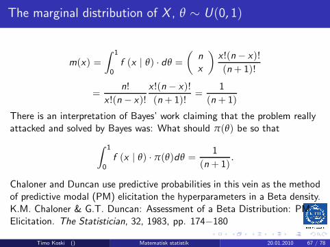
The marginal distribution of X , θ ∼ U(0, 1)
m(x) =
∫ 1
0f (x | θ) · dθ =
(
n
x
)
x !(n − x)!
(n + 1)!
=n!
x !(n − x)!
x !(n − x)!
(n + 1)!=
1
(n + 1)
There is an interpretation of Bayes’ work claiming that the problem reallyattacked and solved by Bayes was: What should π(θ) be so that
∫ 1
0f (x | θ) · π(θ)dθ =
1
(n + 1).
Chaloner and Duncan use predictive probabilities in this vein as the methodof predictive modal (PM) elicitation the hyperparameters in a Beta density.K.M. Chaloner & G.T. Duncan: Assessment of a Beta Distribution: PMElicitation. The Statistician, 32, 1983, pp. 174−180
Timo Koski () Matematisk statistik 20.01.2010 67 / 78
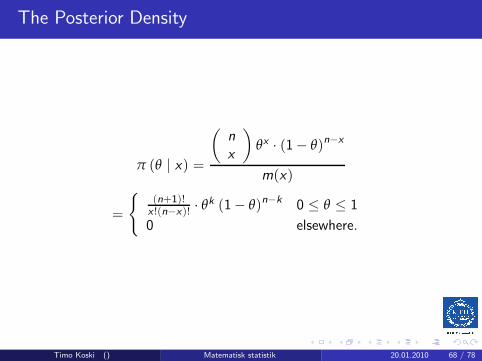
The Posterior Density
π (θ | x) =
(
n
x
)
θx · (1− θ)n−x
m(x)
=
(n+1)!x !(n−x)! · θk (1− θ)n−k 0 ≤ θ ≤ 1
0 elsewhere.
Timo Koski () Matematisk statistik 20.01.2010 68 / 78

The Posterior Density
(n + 1)!
x !(n − x)!=
Γ(n + 2)
Γ(x + 1)Γ(n − x + 1)=
1
B(x + 1, n − x + 1).
Timo Koski () Matematisk statistik 20.01.2010 69 / 78
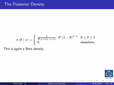
The Posterior Density
π (θ | x) =
1B(x+1,n−x+1) · θx (1− θ)n−x 0 ≤ θ ≤ 1
0 elsewhere.
This is again a Beta density.
Timo Koski () Matematisk statistik 20.01.2010 70 / 78

The Posterior Density θ ∼ Be(α, β)
π (θ | x) =
1B(x+α,n−x+β) · θx+α−1 (1− θ)β+n−x−1 0 ≤ p ≤ 1
0 elsewhere.
This is Beta density Be(α + x , β + n − x) .
Timo Koski () Matematisk statistik 20.01.2010 71 / 78
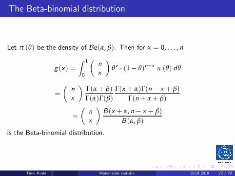
The Beta-binomial distribution
Let π (θ) be the density of Be(α, β). Then for x = 0, . . . , n
g(x) =
∫ 1
0
(
n
x
)
θx · (1− θ)n−x π (θ) dθ
=
(
n
x
)
Γ(α + β)
Γ(α)Γ(β)
Γ(x + α)Γ(n − x + β)
Γ(n + α + β)
=
(
n
x
)
B(x + α, n − x + β)
B(α, β)
is the Beta-binomial distribution.
Timo Koski () Matematisk statistik 20.01.2010 72 / 78

Kullback’s Information Measure
Let f (x) and g (x) be two densities. Kullback’s information measureI (f ; g) is defined as
I (f ; g) :=
∫
Xf (x) log
f (x)
g (x)ν(dx).
We intertpret log f (x)0 = ∞, 0 log 0 = 0. It can be shown that I (f ; g) ≥ 0.
Kullback’s Information Measure does not require the same kind ofconditions for existence as the Fisher information.
Timo Koski () Matematisk statistik 20.01.2010 73 / 78

Kullback’s Information Measure: Two NormalDistributions
Let f (x) and g (x) be densities for N(
θ1; σ2)
, N(
θ2; σ2)
, respectively.Then
logf (x)
g (x)=
1
2σ2
[
(x − θ2)2 − (x − θ1)
2]
I (f ; g) =1
2σ2Eθ1
[
(x − θ2)2 − (x − θ1)
2]
=1
2σ2
[
Eθ1(x − θ2)
2 − σ2]
.
Timo Koski () Matematisk statistik 20.01.2010 74 / 78

Kullback’s Information Measure: Two NormalDistributions
We haveEθ1
(x − θ2)2 = Eθ1
(
x2)
− 2θ2Eθ1(x) + θ2
2
= σ2 + θ21 − 2θ2θ1 + θ2
2 = σ2 + (θ1 − θ2)2 .
Then
I (f ; g) =1
2σ2
[
σ2 + (θ1 − θ2)2 − σ2]
=
=1
2σ2(θ1 − θ2)2 .
I (f ; g) =1
2σ2(θ1 − θ2)
2
Timo Koski () Matematisk statistik 20.01.2010 75 / 78

Kullback’s Information Measure: Natural exponentialdensities
Let fi (x) = h(x)eθi ·x−ψ(θi ), i = 1, 2. Then
I (f1; f2) = (θ1 − θ2) · ∇θψ (θ1) − (ψ (θ1) − ψ (θ2))
Timo Koski () Matematisk statistik 20.01.2010 76 / 78

Summary:
The fact that prior cannot be chosen uniquely is a serious objection toBayesian statistics. Clearly, conjugate priors are perhaps mainly preferredfor mathematical convenience. The question is, how much will the choiceof prior influence the statistical conclusions and decisions ?
Timo Koski () Matematisk statistik 20.01.2010 77 / 78

Robustness and Sensitivity
There are robustness and sensitivity analyses of the impact of choice ofprior on the posterior. Some of this (as known to the lecturer) requiresmathematical tools that are not readily presentable here.
Timo Koski () Matematisk statistik 20.01.2010 78 / 78


