1. A Summary of Export and Import Price Index Methodology A. Introduction 1.1 A price index is a summary measure of the proportionate, or percentage, changes in a set of prices over time. Export and Import Price Indices (XMPIs) measure the overall change in the prices of transactions in goods and services between the residents of an economic territory and residents of the rest of the world. The prices of different goods and services all do not change at the same rate. A price index thus summarizes their movement by averaging over them. A price index assumes a value of unity, or 100, in some reference period. The values of the index for other periods of time show the average proportionate, or percentage, change in prices from the reference period. 1.2 Two basic questions are the focus of this Manual and the associated literature on price indices: • Exactly what sets of prices should be covered by the price index and how should they be collected? • What is the most suitable way in which to average their movements? 1.3 The answer to the first question depends largely on the purposes of the index, which directly connect with the domain of transactions the index is to cover. Distinct price indices associate with different domains of goods and services, such as household consumption, production, investment, and foreign trade flows. Export Price Indices (XPIs) measure changes in the prices of the goods and services provided by the residents of a given economic territory (usually, country) and used by nonresidents (that is, the rest of the world). Import Price Indices (MPIs) measure changes in the prices of goods and services provided by nonresidents (rest of the world) and used by residents of the economic territory. XPIs and MPIs, or XMPIs, are the primary concern of this XMPI Manual. 1.4 In developing a framework for understanding XMPIs, it is useful to consider the principles and practice of the Producer Price Index (PPI) as outlined in the PPI Manual published by the IMF in 2004. As with the PPI, we consider outputs produced by establishments and intermediate consumption or inputs purchased by establishments. By definition, an intermediate input for one establishment is the output of another establishment. From the resident establishments’ perspective, the XPI includes part of the domain of an output PPI, that is, the outputs sold by resident establishments to non-residents and the MPI includes part of the domain of an input PPI, that is, the inputs purchased by resident establishments from non-residents. However, unlike the PPI, XMPIs further include in their domain the outputs of goods and services purchased by, and inputs purchased from, the non- enterprise parts of its government, households, and nonprofit institutional units. This framework is from a resident unit’s perspective and will be seen later in this chapter to serve particular analytical needs. However, XMPIs can also be constructed from a non-resident
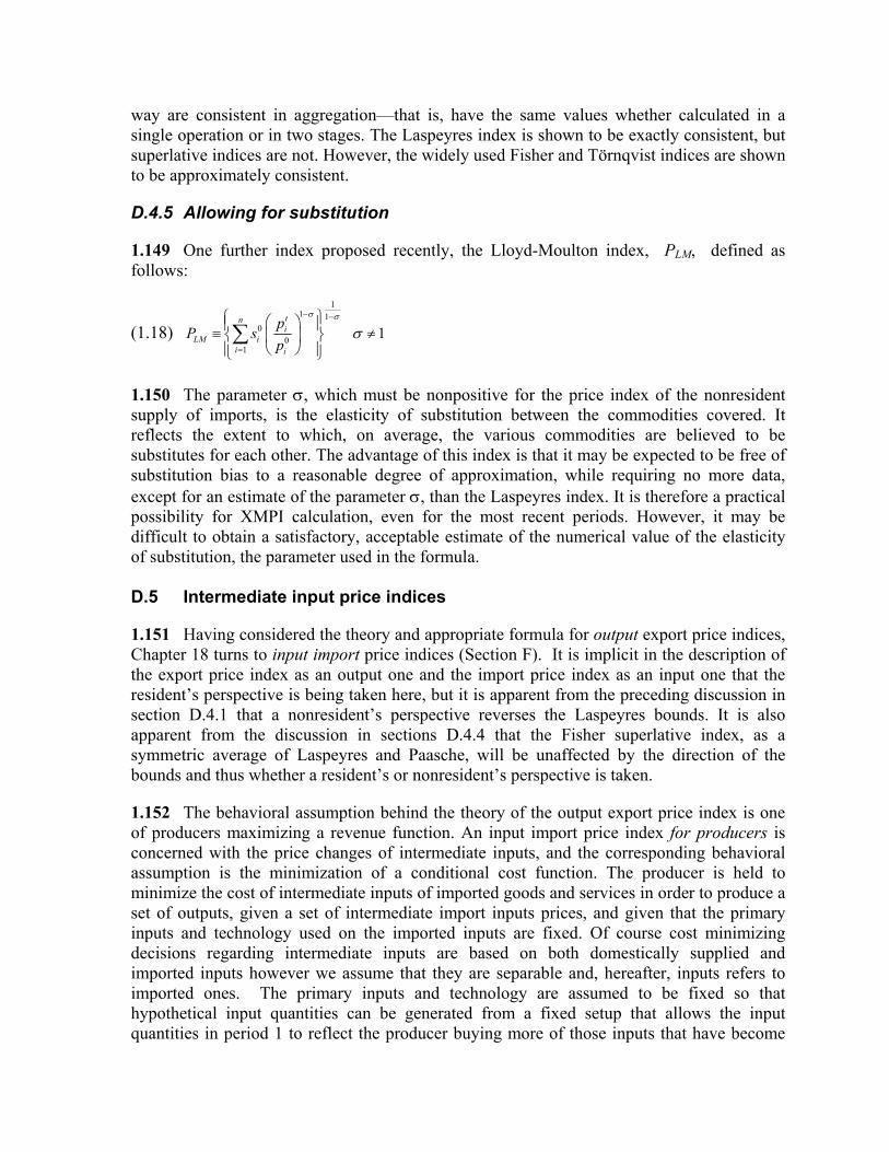
Transcript
1. A Summary of Export and Import Price Index Methodology A. Introduction
1.1 A price index is a summary measure of the proportionate, or percentage, changes in a set of prices over time. Export and Import Price Indices (XMPIs) measure the overall change in the prices of transactions in goods and services between the residents of an economic territory and residents of the rest of the world. The prices of different goods and services all do not change at the same rate. A price index thus summarizes their movement by averaging over them. A price index assumes a value of unity, or 100, in some reference period. The values of the index for other periods of time show the average proportionate, or percentage, change in prices from the reference period.
1.2 Two basic questions are the focus of this Manual and the associated literature on price indices:
• Exactly what sets of prices should be covered by the price index and how should they be collected?
• What is the most suitable way in which to average their movements? 1.3 The answer to the first question depends largely on the purposes of the index, which directly connect with the domain of transactions the index is to cover. Distinct price indices associate with different domains of goods and services, such as household consumption, production, investment, and foreign trade flows. Export Price Indices (XPIs) measure changes in the prices of the goods and services provided by the residents of a given economic territory (usually, country) and used by nonresidents (that is, the rest of the world). Import Price Indices (MPIs) measure changes in the prices of goods and services provided by nonresidents (rest of the world) and used by residents of the economic territory. XPIs and MPIs, or XMPIs, are the primary concern of this XMPI Manual.
1.4 In developing a framework for understanding XMPIs, it is useful to consider the principles and practice of the Producer Price Index (PPI) as outlined in the PPI Manual published by the IMF in 2004. As with the PPI, we consider outputs produced by establishments and intermediate consumption or inputs purchased by establishments. By definition, an intermediate input for one establishment is the output of another establishment. From the resident establishments’ perspective, the XPI includes part of the domain of an output PPI, that is, the outputs sold by resident establishments to non-residents and the MPI includes part of the domain of an input PPI, that is, the inputs purchased by resident establishments from non-residents. However, unlike the PPI, XMPIs further include in their domain the outputs of goods and services purchased by, and inputs purchased from, the non-enterprise parts of its government, households, and nonprofit institutional units. This framework is from a resident unit’s perspective and will be seen later in this chapter to serve particular analytical needs. However, XMPIs can also be constructed from a non-resident
unit’s perspective. Economists are interested in deflating changes in Gross Domestic Product (GDP) (expenditure estimate) over time and one component of this is exports minus imports. A weighted averages of the difference between XPIs and MPIs would serve this purpose. Exports and imports are defined in this context by the 1993 System of National Accounts, Rev. 1, from the rest of the world’s (non-resident’s) perspective: exports are uses of domestic production— input price indices—and imports are the rest of the world’s supply of goods and services to resident users—output price indices. Both the resident’s and non-resident’s perspectives will be outlined as will their analytical uses and implication for measurement, especially with regard to valuation and economic theory.
1.5 Price indices preferably weight the price relative (change) of each specific item they cover by the value share of that item in the transactions domain of the index. For example, an XPI is a weighted average of the price relatives of its components where the weights are the share of each component in the total value of exports covered by the index. Having collected the appropriate set of prices and, the weights, the second question concerns the choice of formula to average the price relatives. Alternative aggregation formulas are considered in Chapters 2, 16–18, and 20–21 of this manual. The price relatives may take the form of ratios of prices between the current and price reference period of specified representative items with detailed commodity descriptions, so that the prices of like are compared with like. Such price relatives can generally only be obtained from establishment surveys. However, unit values for commodity groups may be obtained from customs declarations and their ratios used as “plug ins” for price relatives, a use considered in Chapter 2.
1.6 This chapter provides a general introduction to, and review of, the methods of XMPI compilation. It provides a summary of the relevant theory and practice of index number compilation that helps reading and understanding the detailed chapters that follow, some of which are inevitably quite technical. The chapter starts, as does the Manual, by distinguishing between XMPIs for which the price data are compiled primarily from establishment-survey data and unit value indices that use unit value data from customs documentation as proxies for price data. It considers the merits of each and makes recommendations. The chapter continues to describe the various steps involved in XMPI compilation, starting with the basic concepts, definitions, and purposes of XMPIs. It then discusses the sampling procedures and survey methods used to collect and process the price data, and finishes with the eventual calculation and dissemination of the final indices.
1.7 An introductory presentation of XMPI methods starts with the basic concepts of an XPI and an MPI and the underlying index number theory. This includes the properties and behavior of the various kinds of index numbers that compilers might use. Only after deciding on the most suitable type of index and its coverage based on these theoretical considerations is it possible to go on to determine the best way in which to estimate the index in practice, taking account of the resources available. As noted in the Reader’s Guide, however, the detailed presentation of the relevant index theory appears in later chapters of the Manual because the theory is technically complex when pursued in some depth. The exposition in this chapter does not, therefore, follow the same order as the chapters in the Manual.
1.8 The main topics covered in this chapter are:
• Uses of XMPIs; • Unit value indices and price indices; • Basic index number theory, including the axiomatic and economic approaches to XMPIs; • Elementary price indices; • Transactions, activities, and establishments covered by XMPIs; • Collection and processing of the prices, including adjusting for quality change; • Calculation of XMPIs; • Potential errors and bias; • Organization, management, and dissemination policy; and • An appendix providing an overview of the steps necessary for developing XMPIs. 1.9 It is not the purpose of this introduction to provide a comprehensive summary of the entire contents of the Manual. Thus, not all of the topics treated in the Manual are included in this chapter. The objective of this general introduction is to give a summary presentation of the core issues with which readers need to be acquainted before tackling the detailed chapters that follow.
B. The Uses of XMPIs
1.10 The four principal types of price indices in the system of economic statistics—the consumer price index (CPI), producer price index (PPI), and the XMPIs—are well known and closely watched indicators of macroeconomic performance. They are direct indicators of price inflation for various flows of goods and services. As such, they are also used to deflate series of nominal values of goods and services produced, consumed, and traded to provide measures of changes in their volumes. Consequently, these indices are not only important tools in the design and conduct of the monetary and fiscal policy of the government, but they are also of great utility in informing economic decisions throughout the private sector. They do not, or should not, comprise merely a collection of unrelated price indicators, but provide instead an integrated and consistent view of price developments pertaining to production, consumption, and international transactions in goods and services.
1.11 Like other price indices in the system of price statistics, XMPIs serve multiple purposes. Precisely how they are defined and constructed can very much depend on the data source underlying their construction as well as by whom and for what they are meant to be used. XMPIs can measure either the average change in the price of goods and services as they change ownership between residents of different economic territories, or when they are documented with export declarations or import tariff forms, as they cross national frontiers.
1.12 Uses of XMPIs can be identified from a resident unit’s perspective. A monthly or quarterly XMPI with detailed commodity and industry data allows monitoring of short-term price inflation for different types commodities (henceforth “commodities” refers to goods and services) or through different stages of the resident producer’s production process. Measures of changes in the terms of trade of a country, determined as the ratio of the XPI to the MPI, are used in the determination of changes in the real income of residents. The national accounts identify in the production accounts the output and intermediate consumption (inputs) of resident establishments and these can be decomposed into the output
to residents and to the rest of the world (exports), and the inputs from residents and from the rest of the world (imports). An analysis of the productivity of such establishments requires volume measures of such flows which in turn requires price deflators for exports and imports. In addition, the overall XMPIs for specific commodities can be used to adjust prices of inputs in long-term purchase and sales contracts, a procedure known as “escalation.” Thus an analysis of the transmission of inflation, terms of trade, and productivity of resident establishments, and use for escalation payments by them, is well served by XMPIs.
1.13 Uses of XMPIs can also be identified from a nonresident unit’s perspective. Exports and imports are defined by the 1993 System of National Accounts, Rev. 1 (1993 SNA Rev. 1), from the rest of the world’s (non-resident’s) perspective: exports are the rest of the world’s uses of domestic production and imports are the rest of the world’s supply of goods and services to resident users. Such definitions apply to exports and imports as components of estimates of GDP by expenditure which comprises: household and government expenditure, capital formation, and net exports (exports minus imports) of goods and services. Although XMPIs are an important economic indicator in their own right, a vital use of XMPIs is as a deflator of series of nominal values of exports and imports to derive volume estimates of GDP by the expenditure approach. Thus if XMPIs are to be used as deflators a nonresident unit’s perspective has to be taken and this, as will be seen below and in Chapters 4 and 18, has implications for valuation and economic theory, Beyond their use as deflators, the national accounts framework for XMPIs provides insight into the interlinkages between different price measures. Through net exports, XMPIs directly affect the price index (deflator) of GDP by expenditure. The MPI also contributes to the price changes of intermediate consumption by establishments, the input PPI; the CPI and household consumption deflator; the government consumption deflator; the capital formation deflator; and, through re-exports and goods for processing, the XPI. The XPI contributes to change in the output PPI. As such, the detailed information in XMPIs allow compilers to show the contributions of both the external and internal sources and uses of goods and services to changes in each index of the system of price statistics. Since the price index (deflator) for GDP by the production approach (value added = output – intermediate consumption) is a function of the output and intermediate consumption PPIs, the export and import price indices, viewed in this way, contribute to change in the price index (deflator), not only for GDP by expenditure, but also GDP by production.
1.14 Any remaining part of exports involves the final uses of goods and services by nonresidents. An example is cross-border shopping by nonresident households, which is exports either as nonresident final consumption if the acquired items are consumer goods, or as capital formation if the acquired items are valuables, such as jewelry. Another example is acquisition of second hand productive assets by nonresidents for business purposes, which, besides being shown as exports, also enters as negative capital formation in the domestic, supplying economy, and as capital formation in the using economy.1
1 It is possible, as well, for there to be a generally quite small part of imports not accounted for by nonresident
output involving direct change of ownership of second hand goods and valuables between households resident in different countries. This change of ownership counts as “negative consumption” (consumer durable goods) or negative capital formation (valuables) in the supplying country or territory and positive consumption (consumer
(continued)
1.15 Unlike the PPI, which involves only establishments, or the CPI, which involves only households, the XMPIs potentially involve all types of units in the world economy—not only establishments, but also the nonbusiness parts of general government, households, and nonprofit institutions serving households—for transactions including:
• intermediate consumption and output by business units; • capital formation via acquisition and sales of new and second hand nonfinancial
assets by business units and households if the items transacted are valuables (e.g., works of art and jewelry);
• final consumption of services (e.g., vacation accommodation), as well as of goods via exchange of second hand consumer durables (e.g., automobiles), by non-business parts of nonprofit institutions and government.
1.16 This Manual adopts the System of National Accounts 1993 (1993 SNA) and the Balance of Payments Manual (BPM6) as comprising the conceptual framework for the value aggregates underlying all macroeconomic statistics, including the XMPIs. The desirability of this conceptual concordance between the price indices permits users to clearly understand the linkages between price series, discussed in more detail in Chapter 15. It is this concordance that makes components of the XMPI useful as deflators for exports and imports in the national accounts.
1.17 These varied uses often increase the demand for XMPI data. For example, interest in the XMPI as an indicator of externally generated inflation creates pressure to extend its coverage to include more commodities. While many countries initially develop XMPIs to cover goods in international trade, the XMPIs can and should logically be extended to cover internationally traded services, as noted in Chapters 3, 4, and 15.
C. Unit value indices and price indices
1.18 Export and import unit value indices are based on data from customs documentation and are so named because they take as their building blocks, for individual commodity classes,2 the ratio of the unit value in the current to the base period. They measure, for individual commodity classes, the change over time in the total value of shipments divided by the corresponding total quantity. These elementary level unit value ratios—also, and durables) or capital formation (valuables) in the using territory. Services imports must be provided by nonresident enterprises, and thus count as output of establishments rather than the negative consumption or negative capital formation of nonresident households. 2 The classes used refer to the sub-headings of the Harmonized System which is a complete product classification system designed as a “core” system so that countries adopting it could make further subdivisions according to their particular tariff and statistical needs. At the international level, the Harmonized System consists of approximately 5,000 article descriptions which appear as headings and subheadings. Countries can add more detailed subdivisions for classifying goods for tariff, quota or statistical purposes so long as any such subdivision is added and coded at a level beyond the 6-digit numerical code provided in the Harmonized System. Coding beyond the 6-digit level is usually at the 8-digit level and is generally referred to as the “national level,” see Chapter 4 for details.
hereafter, referred to as (elementary) unit value indices—are subsequently aggregated across commodity classes using standard weighted index number formulas where the weights are the relative shares of the commodity group in total exports/imports. Export and import price indices have as their building blocks at the elementary level the price change of well-defined representative items based on establishment surveys. Export and import unit value indices by necessity differ from price indices because of their source data. A unit value elementary index, PU, is given for a price comparison between the current period t and a reference period 0 over m=1, ....,M items in period t and over n=1, ....,N items in period 0 by:
(1.1) PU ≡0 0
1 1
0
1 1
M Nt tm m n n
m nM N
tm n
m n
p q p q
q q
= =
= =
⎛ ⎞ ⎛ ⎞⎜ ⎟ ⎜ ⎟⎜ ⎟ ⎜ ⎟⎜ ⎟ ⎜ ⎟⎜ ⎟ ⎜ ⎟⎝ ⎠ ⎝ ⎠
∑ ∑
∑ ∑
where prices and quantities are given respectively by tmp and t
mq for period t, and 0np and 0
nq for period 0.
1.23 Unit value indices are used to represent price changes and the probity of their use is reliant on the homogeneity of the items transacted within the classification classes for which transactions are aggregated and the related issue of how tightly the classification classes are themselves defined. Unit value indices work well for the aggregation of identical, homogeneous, items, but are biased for the aggregation of different, heterogeneous, goods. Consider, for example, the prices of two heterogeneous goods A and B at 10 and 12 in the reference period that remain constant over time, but with a shift in quantities from say 6, for both A and B in the reference period, to 8 for A and 4 for B in the current period. The correct answer for any price index number formula would give an answer of unity, no overall price change. However, the unit values would fall by 3 per cent reflecting the shift in the quantity basket in the current period from the higher price level of 12 for A to the lower price level of 10 for B. This unit value bias arise from a compositional shift in the basket of items transacted. Of note is that if A and B were homogeneous items, there would be no bias. The unit value index would be the correct measure reflecting the fact that the same item has become, on average, cheaper. The problem for XMPI compilers is that unit values from customs documentation has the appeal of a relatively cheap and easily available administrative source of data, compared with pricing representative items from establishments, but the classification classes used are not sufficiently detailed to ensure that the prices of like in one month are compare with like in the next. Compositional changes within a classification group in the qualities of goods exported or imported from one month to the next can change and unit value indices, as can be seen from equation (1.10), do not just measure pure price changes: they are influenced by changes in relative quantities.
1.24 Customs data can usually be reliably used for information on the relative values of goods imported and exported to be used to weight the price changes. Data on the values of goods imported and exported measured in current prices do not suffer from unit value bias. Customs data may be supplemented with data from other sources for weights including establishment surveys (see Chapter 5). Customs documents can also be used in the development of a sampling frame of establishments using the details on the documents of the establishments responsible for the trade (see Chapter 6).
C.1 Unit value indices and their suitability for aggregation over homogeneous items
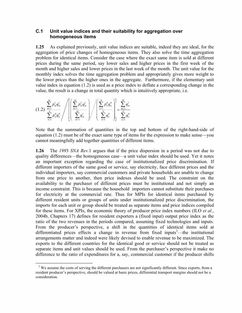
1.25 As explained previously, unit value indices are suitable, indeed they are ideal, for the aggregation of price changes of homogeneous items. They also solve the time aggregation problem for identical items. Consider the case where the exact same item is sold at different prices during the same period, say lower sales and higher prices in the first week of the month and higher sales and lower prices in the last week of the month. The unit value for the monthly index solves the time aggregation problem and appropriately gives more weight to the lower prices than the higher ones in the aggregate. Furthermore, if the elementary unit value index in equation (1.2) is used as a price index to deflate a corresponding change in the value, the result is a change in total quantity which is intuitively appropriate, i.e.
Note that the summation of quantities in the top and bottom of the right-hand-side of equation (1.2) must be of the exact same type of items for the expression to make sense—you cannot meaningfully add together quantities of different items.
1.26 The 1993 SNA Rev.1 argues that if the price dispersion in a period was not due to quality differences—the homogeneous case—a unit value index should be used. Yet it notes an important exception regarding the case of institutionalized price discrimination. If different importers of the same good or service, say electricity, face different prices and the individual importers, say commercial customers and private households are unable to change from one price to another, then price indexes should be used. The constraint on the availability to the purchaser of different prices must be institutional and not simply an income constraint. This is because the household importers cannot substitute their purchases for electricity at the commercial rate. Thus for MPIs for identical items purchased by different resident units or groups of units under institutionalized price discrimination, the imports for each unit or group should be treated as separate items and price indices compiled for these items. For XPIs, the economic theory of producer price index numbers (ILO et al., 2004b, Chapters 17) defines for resident exporters a (fixed input) output price index as the ratio of the two revenues in the periods compared, assuming fixed technologies and inputs. From the producer’s perspective, a shift in the quantities of identical items sold at differentiated prices effects a change in revenue from fixed inputs3—the institutional arrangements matter and indeed were likely devised to enable revenue to be maximized. The exports to the different countries for the identical good or service should not be treated as separate items and unit values should be used. From the purchaser’s perspective it make no difference to the ratio of expenditures for a, say, commercial customer if the producer shifts
3 We assume the costs of serving the different purchasers are not significantly different. Since exports, from a
resident producer’s perspective, should be valued at basic prices, differential transport margins should not be a consideration.
some of its quantities to private households—the institutional arrangements do not matter and unit values should not be used. In other words, from the viewpoints of the purchasers of the above homogeneous commodity, what counts is his or her (separate from other purchasers) unit value price, not the overall unit value price across all purchasers, which would be the relevant price for the seller.
1.27 Price comparisons may be required for aggregation across comparable, but not identical, items, say electricity exported to different countries at different prices and price changes. It may be that the some of the price difference can be attributed to the reliability of the supply. If the effect of quality differences on price dispersion was small, unit values may be used as long as the differential quality difference can be stripped from the prices, say using explicit estimate of the effect on price of the differences in supply quality. Quality adjustments to prices are a standard part of index number work and Chapter 8 outlines the methods available to undertake such adjustments.
C.2 Errors and bias in the use of unit value indices
1.28 Unit value indices derived from data collected by customs authorities are used by many countries as surrogates for price changes at the elementary level of aggregation. The following are grounds upon which unit value indices can be deemed to be potentially unreliable: • Bias arises from compositional changes in quantities and quality mix of what is exported
and imported. Even with best practice stratification the scope for reducing such bias is limited due to the sparse variable list—class of (quantity) size of the order and country of origin/destination)—available on customs documents. Indeed it does not follow that such breakdowns are always beneficial;
• For unique and complex goods, model pricing can be used in establishment-based surveys where the respondent is asked to price each period a commodity, say a machine with fixed specified characteristics. This possibility is not open to unit value indices;
• Methods for appropriately dealing with quality change, temporarily missing values, and seasonal goods can be employed with establishment-based surveys to an extent that is not possible with unit value indices;
• The information on quantities in customs returns, and the related matter of choice of units in which the quantities are measured, has been found in practice in the past to be seriously problematic, though the advent of computer systems has been a major innovation in mitigating such problems—the Automated System for Customs Data (ASYCUDA) project4 of United Nations Conference on Trade and Development (UNCTAD)has applied computerized systems in the customs administrations of the least developed countries;
4 ASYCUDA is functioning in about 90 developing countries. That system verifies declaration entries
immediately. Declarations need to be completely filled in order to receive customs clearance. This means among others that quantity information is required. In addition, customs values are validated – to avoid undervaluation – using unit values on the declaration which are matched against a pre-determined list of commodity prices.
• With customs unions countries may simply have limited or no intra-area trade data to use; • An increasing proportion of trade is in services and by e-trade and not subject to customs
documentation; • Unit value indices rely to a large extent on outlier detection and deletion. Given the
stickiness of many price changes, such deletions run the risk of missing the large price catch-ups when they take place and understating inflation;
• Valuation requirements for deflation of the aggregates of the United Nations (1993) System of National Accounts (SNA) are determined for unit value indices by customs procedures which are not in accord with the accrual principle of the SNA 1993 REV.1.
1.29 A main advantage of the use of unit value indices is held to be their coverage and relatively low resource cost. However, such coverage should not be assumed for all classes since the unit values used may effectively be non-random samples and exclude: commodities traded irregularly; that have no quantity reported (especially for parts and machinery); have low value shipments; and erratic month-to-month changes. The extent of such exclusions may be substantial,. Establishment-based surveys can be quite representative. Often a small number of wholesalers or establishments are responsible for much of the total value of imports or exports and, assuming cooperation, will be a cost-effective source of reliable data. Further, good sampling can, by definition, realize accurate price change measures. Finally, the value shares of exports and imports, obtained from customs data, which generally has good coverage of merchandise trade, will form the basis of the information used for weights for establishment-based price survey data.
1.30 Alternative index number formula are usually assessed by determining how well they satisfy a number of reasonable properties, the axiomatic approach. Chapters 17 and 21 outline and apply such tests to compares the performance of a number of index number formulas used at the higher and elementary level respectively. Unit value indices fail the identity test—if all prices remain constant the value of the index should be unity—and the proportionality test—a proportional change in all prices should result in the same proportional change in the index; both tests are regarded as important tests in index number theory. Unit value indices also fail the commensurability test—a price index should be invariant to the units of measurement selected, for example, if the measurement of one or more of the items changed from pounds weight to kilograms, the index should not change. In practice the units of measurement for an item in a detailed classification group are generally the same for customs documentation, however, quality variations are equivalent to changes in units of measurement, for example 20 automobiles are not equivalent to 20 automobiles with larger engines, and in this sense failure of the commensurability test is an important deficiency of unit value indices derived from customs documentation.
1.31 Alternative index number formula can also be assessed by the economic approach, as outlined in Chapter 18. Chapter 2 also notes that an index that uses unit value changes as “plug ins” for price changes will only equate to a theoretical economic index number under restrictive conditions.
1.32 The Fisher index number formula, as will be outlined below and in detail in Chapters 16–18, has been described as “ideal” on the grounds that it satisfies all reasonable tests required of index numbers, and “superlative” on the grounds that it, along with a few other
such formula, approximates well an index well-defined in economic theory that has good properties. An important question is: are the conditions for a unit value index to equal a Fisher index likely to hold in practice? In Chapter 2 it is shown that such conditions are all highly restrictive. They are that either: (i) all prices are equal in each period; or (ii) all quantity relatives are equal; or (iii) price relatives and quantity relatives are uncorrelated.
C.3 Evidence of errors and bias in using unit value indices based on customs data
1.33 Given the potential for errors and bias in the use of unit value indices based on customs data, it is important to consider the evidence for such errors and bias in practice. A number of countries have compiled unit value indices using customs data alongside price indices based on establishment surveys. Establishment–based price indices by their nature are compiled by first, determining with the responding establishments detailed price-determining specifications of representative commodities, and their prices in the reference period on “price initiation,” and then comparing the prices of the same specifications in subsequent periods.5 In this important regard the cited studies ask: how well do unit value indices stand up against price indices designed to overcome one of their major failings? While there are methodological caveats in comparing the two series, including differences in formulas used, the overriding conclusion from the evidence summarized in Chapter 2 is that there are substantial differences between the two. Changes in unit value based indices of exports and imports do not represent those of their corresponding price indices and further, can be very misleading as indicators of such price indices. This holds for month-on-month and long run annual changes with differences compounding for terms of trade indices. Such findings have led the statistical authorities in most of the countries studied to abandon the use of unit value indices. 1.34 As noted in Section C.2 above, the concern arises not only because of the potential for errors and biases from the use of unit value indices based on customs data, but also because (i) not all customs returns may have suitable quantity data with the result that the coverage of the unit value is arbitrarily reduced; (ii) some unit value changes are often highly volatile and automatic or otherwise deletion routines may be unsatisfactory in that they may remove some of the signal as well as the noise; (iii) countries joining customs unions may no longer have customs data for much of their trade; (iv) customs data do not cover trade in services and e-commerce, as well as trade in electricity, gas and water for which establishment surveys are generally used; (v) for many commodity classes the turnover in differentiated items each month is substantial and customs data are inappropriate for the treatment of quality changes, new goods, missing goods, seasonal goods, and hard-to-measure goods such as one-off machine and ships; and (vi) the valuation requirements of the 1993 SNA Rev.1 for trade price indices to be used as deflators for national accounts
5 There remains a problem for both types of data when a commodity changes, say a new improved model is
introduced. Unit value indices will be biased upwards. A change in the detailed specifications will be noted when using establishments surveys and the methods in Chapters 8 and 9 are available to deal with the quality change/new good.
aggregates, as outlined in Chapter 4, are better met by data from establishment surveys than customs data. C.4 Strategic options for the compilation of XMPIs
1.35 Given there is a serious cause for concern in using unit value indices based on customs data for XMPIs there is the practical matter of the strategic options open to statistical authorities that use such data. Unit value indices are used by many countries and a move to price indices based on establishment surveys has resource consequences. One possibility is to identify whether there are particular commodities less prone to unit value bias and utilize unit value indices only for these sub-aggregates in a hybrid overall index. Chapter 2 outlines the methodology for the construction of such indices. The use of hybrid indices has the resource advantage of undertaking price surveys only for commodities for which they are necessary. The efficacy of such advice depends on the extent to which reliable unit value indices will be available at a disaggregated level. 1.36 This Manual advises that countries using unit value indices undertake a staged progressive adoption of hybrid indices with, over time, increasing proportions of unit value indices being substituted in favor of establishment-based survey data. An appraisal should be undertaken of each commodity group to determine the most resource efficient and methodologically appropriate source data. One issue regarding the homogeneity of sub-headings the testing customs elementary aggregates for multiple elementary items and Chapter 6 section C provides some guidelines in this regard. Nonetheless, the long-term goal should be XMPIs that are primarily base on establishment surveys. 1.37 Preference should be given to the use of establishment survey data for the “low hanging fruit” of establishments responsible for relatively high proportions of exports and imports, some of which may be owned by the state and may have some reporting obligation. Likely examples of such commodity groups include natural gas, petroleum, electricity, and airlines. There will also be industries in which unit values indices are prima facie inadequate measures of price changes, largely because of the churn in highly differentiated commodities, or the custom-made nature of the commodities, such as shipbuilding and oil platforms. Further, there may be industries which account for a substantial proportion of trade and the pay off of reliable data far outweighs the survey costs, for example, the use of surveys of fish-processing plants for major exporters of fish commodities and of agricultural marketing cooperatives for exports of primary commodities. 1.38 Source data for XMPIs other than customs unit values and establishment surveys include mirror price indices, that is the corresponding series from other countries—if your major exports (imports) are to (from) one or more identified countries and these countries have what you believe to be reliable import (export) price indices for these goods, then a weighted average of these series may be a suitable proxy. A further alternative is to use international commodity price indices to proxy exports or imports price changes. The assumption is that there is a global market in which countries are price takers with little to no price discrimination between countries. Similar considerations apply to the use of price series produced by a resource rich country for hard-to-measure goods and services, such as personal computers, that have benefited from quality adjustment procedures. A country may have a
program for compiling an establishment-based output (input) producer price index (PPI) that is a measure of the price changes of the output from (input to) the domestic economy as a whole to (from) both the resident and non-residents. In some cases the establishments may wholly sell to (buy in from) non-resident markets, or not practice price discrimination between the two markets (assuming relevant transportation, tax and other margins are constant or insignificant)6 in which case a timely series should exist for XMPIs. Or it may be that price changes for a difficult or costly to measure commodity group can be imputed from another group. 1.39 A gradualist approach has two potential problems. The first is that its reliance on unit value indices for what may be major commodity classes is unlikely to be soundly based. Chapter 2 examines some evidence on the reliability of unit value indices for particular commodity groups. The evidence is not supportive of there being many sub-headings for which unit values indices can be relied upon. The case for adopting hybrid indices is a pragmatic one arising from resource and expertise constraints to the adoption of an establishment survey-based XMPIs. A second, potential problem with a gradualist approach is longer-term changes in the index become problematic. The user cannot judge how much of the long run change is due to changes in the indicator series used. A gradualist approach should be accompanied by well-signaled steps to users and, when changed, by back data for at least the last 12 months so that 12-month changes can be identified and the new index readily linked to the old. There should be adequate meta data to explain the change. The approach is inferior to a strategy that simply requires the adoption of a primarily establishment-based price index. The culmination of a program of use of hybrid indices should be an index in which unit values have little or no place. 1.40 Of course improvements to unit value indices should be made as possible. These would include more detailed stratification including shipments by/to (major) establishments to/from given countries. However, the absence on customs documentation of highly detailed commodity descriptions by which to stratify unit values precludes any stratification that allows the compiler to be confident that like in any month is compared with like in the next. Improved outlier detection routines are certainly advocated by the Manual when unit value indices are used (see Chapter 6 Section C). However, caution is expressed about the efficacy of such routines unless well applied and need for validation prior to deletion with an exporting/importing establishment or other third-party source is strongly recommended. Deletion routines should be used to identify unusual price changes, which then have to be followed up to ensure that they are not real changes—large catch-up price changes under sticky price-setting—but due to wrongly entered numbers or a change in the units for quantities. However, the sheer magnitude of the task of following up the original customs documentation, and then possibly having to refer back to the exporter/importer, may well preclude detailed follow-ups with an over reliance on automatic deletion routines. Second, such routines will be based on past parameters of the dispersion, which may themselves be
6 From a resident’s perspective exports transportation costs should be excluded for export price indices
because the pricing basis is the basic price—that is, the amount received by the producer, or distributor exclusive of any taxes on commodities and transport and trade margins, while from the nonresident’s perspective the pricing basis for imports is the basic price.
based on outliers. Further, the parameters may themselves be unstable, say due to sticky pricing and volatile exchange rates, and past experience not be useful for future deletion practice. Finally, there is the arbitrary nature of the cut-off values often used in practice for deletion. 1.41 The main problem with simply introducing a new establishment survey-based program is the resource cost. This includes the training of price collectors, building of sample frames, sample selection of items and establishments, computer routines, data validations and much more that is the subject of Chapters 3–14 of this manual. However, if a PPI program is already established, there will be synergies with the external trade price index program including computer routines, price collecting manuals and training, expertise in sampling items and establishments. There will be some commodity groups for which the PPI results are alone sufficient. However, in other commodity groups for which the current PPI sample is not sufficiently detailed to allow reliable export /import indices to be compiled, the sample of items/establishments will need to be supplemented to include items that are imported/exported. Chapter 13 considers some organizational issues in taking advantage of the synergies between the two programs.
D. Basic index number formulas and the axiomatic and economic approaches to XMPIs
D.1 Basic index number formulas
1.42 While the collection of monthly/quarterly data on unit value or price changes at a detailed level is a natural prerequisite for the compilation of XMPIs, as is the collection of data on relative value shares to weight the price changes, an important question to decide on is the kind of index number formula to use when aggregating the data collected. Index number formulas that involve weights are referred to as being used at the higher level of aggregation. Thus the subject matter of such weighted index number formulas discussed in this section applies to XMPIs whether compiled using unit value indices derived from customs data at the lower (elementary) level or the price changes of well defined representative goods and services from establishment surveys at the lower level. Both provide elementary indices at the detailed commodity classification and are aggregated at the higher level using an index number formula that is weighted. The extensive list of references given at the end of this Manual reflects the large literature on this subject. Many different mathematical formulas have been proposed over the past two centuries. Nevertheless, there is now a broad consensus among economists and compilers of XMPIs about what is the most appropriate type of formula to use, at least in principle. While the consensus has not settled for a single formula, it has narrowed to a very small class of superlative indices. A characteristic feature of these indices is that they treat the prices and quantities in both periods being compared symmetrically. They tend to yield very similar results and behave in very similar ways.
1.43 However, in some cases, there may not be sufficient information on the quantities and nominal flows (i.e., the weights) of internationally traded goods and services in the current period to calculate a symmetric, or superlative, index. It may be necessary to resort to
second-best alternatives in practice, but in order to be able to make a rational choice between the various possibilities, it also is necessary to have a clear idea of the target index that would be preferred, in principle. The target index can have considerable influence on practical matters such as the frequency with which the weights used in the index should be updated.
1.44 The Manual provides a comprehensive, rigorous, and up-to-date discussion of relevant index number theory. Several chapters from Chapter 16 onward are devoted to detailed explanations of index number theory from both a statistical and an economic perspective. The main points are summarized in the following sections. Many propositions or theorems are stated without proof in this chapter because the proofs are given or referenced in later chapters to which the reader can easily refer in order to obtain full explanations and a deeper understanding of the points made. There are numerous cross-references to the relevant sections in later chapters.
D.1.1 Price indices based on baskets of goods and services
1.45 The purpose of an index number may be explained from the resident’s perspective by comparing the values of the supply of exports or the uses of imports of goods and services in two time periods. Knowing that the value of exports has increased by say 5 percent is not very informative if we do not know how much of this change is due to changes in the prices of the goods and services and how much to changes in the quantities produced. The purpose of an index number is to decompose proportionate or percentage changes in value aggregates into their overall price and quantity change components. XMPIs are intended to measure the price component of the change. One way to do this is to measure the change in the value of an aggregate by holding the quantities constant.
D.1.2 Lowe indices
1.46 One very wide, and popular, class of price indices is obtained by defining the index as the percentage change between the periods compared in the total cost of producing a fixed set of quantities, generally described as a “basket.” The meaning of such an index is easy to grasp and to explain to users. This class of index is called a Lowe index in this Manual after the index number pioneer who first proposed it in 1823 (see Section B.2 of Chapter 16). Most statistical offices make use of some kind of Lowe index in practice. It is described in some detail in Sections D.1 and D.2 of Chapter 16.
1.47 In principle, any set of goods and services could serve as the basket. The basket does not have to be restricted to the basket actually produced or used in one or other of the two periods compared. For practical reasons, the basket of quantities used for XMPI purposes usually has to be based on customs data and a survey of establishment revenues (costs) from exports (imports) conducted in an earlier period than either of the two periods whose prices are compared, simply because it takes time to compile and adopt the data. For example, a monthly XMPI may run from January 2008 onward, with January 2008 = 100 as its price reference period, but the quantities may be derived from customs/establishment-survey value data from an earlier period. The basket also may refer to a year or average of more than one year whereas the price reference period for the index may be a year, month or quarter.
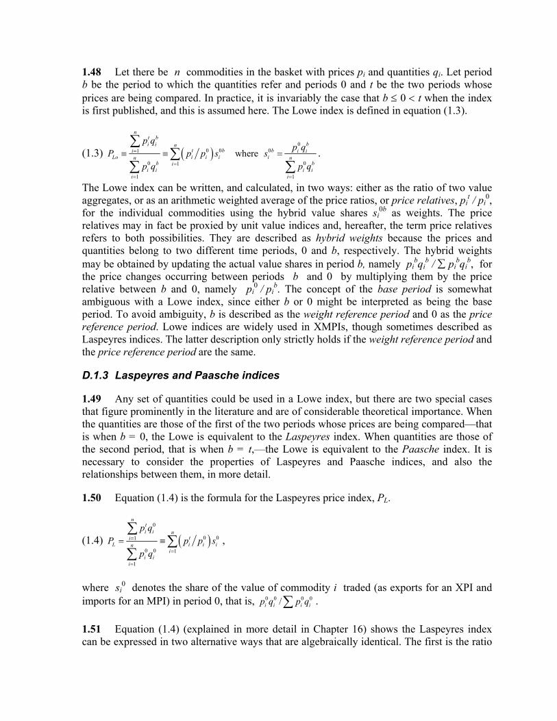
1.48 Let there be n commodities in the basket with prices pi and quantities qi. Let period b be the period to which the quantities refer and periods 0 and t be the two periods whose prices are being compared. In practice, it is invariably the case that b ≤ 0 < t when the index is first published, and this is assumed here. The Lowe index is defined in equation (1.3).
(1.3) ( )0
0 0 01
0 01
1 1
where
nt b
bi i nt b bi i i
Lo i i i in nb bi
i i i ii i
p qp q
P p p s sp q p q
=
=
= =
≡ ≡ =∑
∑∑ ∑
.
The Lowe index can be written, and calculated, in two ways: either as the ratio of two value aggregates, or as an arithmetic weighted average of the price ratios, or price relatives, pi
t / pi0,
for the individual commodities using the hybrid value shares si0b as weights. The price
relatives may in fact be proxied by unit value indices and, hereafter, the term price relatives refers to both possibilities. They are described as hybrid weights because the prices and quantities belong to two different time periods, 0 and b, respectively. The hybrid weights may be obtained by updating the actual value shares in period b, namely pi
bqib / ∑ pi
bqib, for
the price changes occurring between periods b and 0 by multiplying them by the price relative between b and 0, namely pi
0 / pib. The concept of the base period is somewhat
ambiguous with a Lowe index, since either b or 0 might be interpreted as being the base period. To avoid ambiguity, b is described as the weight reference period and 0 as the price reference period. Lowe indices are widely used in XMPIs, though sometimes described as Laspeyres indices. The latter description only strictly holds if the weight reference period and the price reference period are the same.
D.1.3 Laspeyres and Paasche indices
1.49 Any set of quantities could be used in a Lowe index, but there are two special cases that figure prominently in the literature and are of considerable theoretical importance. When the quantities are those of the first of the two periods whose prices are being compared—that is when b = 0, the Lowe is equivalent to the Laspeyres index. When quantities are those of the second period, that is when b = t,—the Lowe is equivalent to the Paasche index. It is necessary to consider the properties of Laspeyres and Paasche indices, and also the relationships between them, in more detail.
1.50 Equation (1.4) is the formula for the Laspeyres price index, PL.
(1.4) ( )0
0 01
0 0 1
1
nti i n
tiL i i in
ii i
i
p qP p p s
p q
=
=
=
= ≡∑
∑∑
,
where si
0 denotes the share of the value of commodity i traded (as exports for an XPI and imports for an MPI) in period 0, that is, 0 0 0 0/i i i ip q p q∑ . 1.51 Equation (1.4) (explained in more detail in Chapter 16) shows the Laspeyres index can be expressed in two alternative ways that are algebraically identical. The first is the ratio
of the values of the basket of producer goods and services traded in period 0 when valued at the prices of periods t and 0, respectively. The second is a weighted arithmetic average of the ratios of the individual prices in periods t and 0 using the traded value shares in period 0 as weights. The individual price ratios, (pi
t/pi0), are described as price relatives—though they
may be proxied by unit value indices. Statistical offices often calculate XMPIs using the second formula by recording the changes in the prices of goods and services exported and imported and weighting them by the traded value shares in the base period 0.
1.52 A Young index is similar to the right hand side Laspeyres weighted average of price changes given in equation (1.4), but instead of using period 0 weights, uses earlier period b traded value shares as weights due to the lack of timely information on the former.
1.53 Equation (1.5) is the formula for the Paasche index, PP.
(1.5) ( )1
101
0 1
1
nt ti i n
t tiP i i in
t ii i
i
p qP p p s
p q
−−=
=
=
⎧ ⎫= ≡ ⎨ ⎬⎩ ⎭
∑∑
∑,
where si
t denotes the actual share of traded values of commodity i in period t, that is, pi
tqit / ∑ pi
tqit The Paasche index can also be expressed in two alternative ways: either as the
ratio of two value aggregates or as a weighted average of the price relatives, the average being a harmonic average that uses the traded value shares of the later period t as weights. However, it follows from equation (1.3) that the Paasche index can also be expressed as a weighted arithmetic average of the price relatives using hybrid weights in which the quantities of t are valued at the prices of 0. 1.54 If the objective is simply to measure the price change between the two periods considered in isolation, there is no reason to prefer the basket of the earlier period to that of the later period, or vice versa. Both baskets are equally relevant. Both indices are equally justifiable, or acceptable, from a conceptual point of view. In practice, however, XMPIs are calculated for a succession of time periods. Time series of monthly Laspeyres XMPIs based on period 0 benefit from requiring only a single set of nominal trade weights, those of period 0, so that only the prices have to be collected on a regular monthly basis. Time series of Paasche XMPIs, on the other hand, requires data on both prices and quantities (or nominal trade weights) in each successive period. Thus, it is much less costly, and time consuming, to calculate a time series of Laspeyres indices than a time series of Paasche indices. If detailed data on nominal trade flows are not timely, this is a decisive practical advantage of Laspeyres (as well as Lowe) indices over Paasche indices and explains why Laspeyres, Young, and Lowe indices are used much more extensively than Paasche indices. Monthly Laspeyres, Young, or Lowe XMPIs can be published as soon as the price information has been collected and processed, since the base period weights are already available. Of course, weights should be updated regularly and Laspeyres indices with frequently updated weights, or annual chained Laspeyres indices, are a preferred option as discussed below.
D.1.4 Decomposing current value changes using Laspeyres and Paasche
1.55 Laspeyres and Paasche volume indices are defined in a similar way to the price indices, simply by interchanging the ps and qs in formulas (1.4) and (1.5). They summarize changes over time in the flow of quantities of goods and services exported/imported. A Laspeyres volume index values the quantities at the fixed prices of the earlier period, while the Paasche volume index uses the prices of the later period. The ratio of the nominal (current price) traded values in two periods (V) reflects the combined effects of both price and quantity changes. When Laspeyres and Paasche indices are used, the value change exactly decomposes into a price index times a volume index only if the Laspeyres price (volume) index is matched with the Paasche volume (price) index. Let PL and QL denote the Laspeyres price and volume indices and let PP and QP denote the Paasche price and volume indices. As shown in Chapter 16, PL × QP ≡ V and PP × QL ≡ V. It follows that volume series ca be defined as / LV P or / PV P . This division of a value change by price index to form a volume index is referred to as deflation. If a Paasche deflator is used for comparisons between say period 0 and successive periods this yields on deflation a Laspeyres volume series that measures quantities at a constant period 0 prices.
1.56 Suppose, for example, compilers want to deflate a time series of imports in the national accounts to measure changes in import volume supplied to the economy at constant prices over time. To generate a series of import values at constant base period prices (whose movements are identical with those of the Laspeyres volume index), the imports at current prices must be deflated by a series of Paasche price indices. Laspeyres MPIs would not be appropriate for the purpose. If nominal values are available and deflated at a very low level of disaggregation, the resulting volume series for the detailed trade commodities can then be aggregated up using a say (chained) Laspeyres formula.
D.1.5 Ratios of Lowe and Laspeyres indices
1.57 The Lowe index is transitive. The ratio of two Lowe indices using the same set of qbs is also a Lowe index. For example, the ratio of the Lowe index for period t + 1 with price reference period 0 divided by that for period t also with price reference period 0 is:
(1.6) 1 0 1
, 11 1 1
0
1 1 1
n n nt b b t bi i i i i i
t ti i iLon n n
t b b t bi i i i i i
i i i
p q p q p qP
p q p q p q
+ +
+= = =
= = =
= =∑ ∑ ∑
∑ ∑ ∑
1.58 This is a Lowe index for period t + 1, with period t as the price reference period. This kind of index is, in fact, widely used to measure short-term price movements, such as between t and t + 1, even though the quantities may date back to some much earlier period b.
1.59 A Lowe index can also be expressed as the ratio of two Laspeyres indices. For example, the Lowe index for period t with price reference period 0 is equal to the Laspeyres index for period t with price reference period b divided by the Laspeyres index for period 0 also with price reference period b. Thus,
(1.7) 1 1 10
0 0
1 1 1
n n nt b t b b b
ti i i i i ii i i L
Lo n n nb b b b L
i i i i i ii i i
p q p q p qPPPp q p q p q
= = =
= = =
= = =∑ ∑ ∑
∑ ∑ ∑.
D.1.6 Updated Lowe indices
1.60 It is useful to have a formula that enables a Lowe index to be calculated directly as a chain index in which the index for period t + 1 is obtained by updating the index for period t. Because Lowe indices are transitive, the Lowe index for period t + 1 with price reference period 0 can be written as the product of the Lowe index for period t with price reference period 0 multiplied the Lowe index for period t + 1 with price reference period t. Thus,
1.61 Hybrid weights of the kind defined in equation (1.9) are often described as price updated weights. They can be obtained by adjusting the original weights pi
bqib/ ∑pi
bqib by the
price relatives pit / pi
b. By price updating the weights from b to t in this way, the index between t and t + 1 can be calculated directly as a weighted average of the prices relatives pi
t+1 / pit without referring back to the price reference period 0. The index can then be linked
on to the value of the index in the preceding period t.
D.1.7 Interrelationships between fixed basket indices
1.62 Consider first the interrelationship between the Laspeyres and the Paasche indices. A well-known result in index number theory is that if the price and quantity changes (weighted by values) are negatively correlated, then the Laspeyres index exceeds the Paasche. Conversely, if the weighted price and quantity changes are positively correlated, then the Paasche index exceeds the Laspeyres. The proof is given in Appendix 16.1 of Chapter 16.
1.63 This has different implications for purchasers and suppliers. The theory of purchasing behavior indicates that, as users of goods and services, producers and consumers typically react to price changes by substituting goods or services that have become relatively cheaper for those that have become relatively dearer. Thus they purchase smaller quantities of the higher-priced commodities and more of lower-priced ones. This is known as the substitution effect, and it implies a negative correlation between the price and quantity relatives. In this
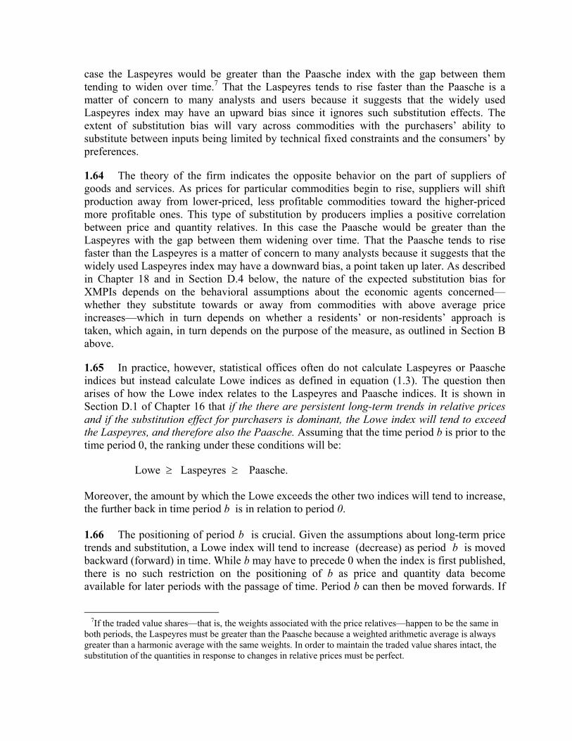
case the Laspeyres would be greater than the Paasche index with the gap between them tending to widen over time.7 That the Laspeyres tends to rise faster than the Paasche is a matter of concern to many analysts and users because it suggests that the widely used Laspeyres index may have an upward bias since it ignores such substitution effects. The extent of substitution bias will vary across commodities with the purchasers’ ability to substitute between inputs being limited by technical fixed constraints and the consumers’ by preferences.
1.64 The theory of the firm indicates the opposite behavior on the part of suppliers of goods and services. As prices for particular commodities begin to rise, suppliers will shift production away from lower-priced, less profitable commodities toward the higher-priced more profitable ones. This type of substitution by producers implies a positive correlation between price and quantity relatives. In this case the Paasche would be greater than the Laspeyres with the gap between them widening over time. That the Paasche tends to rise faster than the Laspeyres is a matter of concern to many analysts because it suggests that the widely used Laspeyres index may have a downward bias, a point taken up later. As described in Chapter 18 and in Section D.4 below, the nature of the expected substitution bias for XMPIs depends on the behavioral assumptions about the economic agents concerned—whether they substitute towards or away from commodities with above average price increases—which in turn depends on whether a residents’ or non-residents’ approach is taken, which again, in turn depends on the purpose of the measure, as outlined in Section B above.
1.65 In practice, however, statistical offices often do not calculate Laspeyres or Paasche indices but instead calculate Lowe indices as defined in equation (1.3). The question then arises of how the Lowe index relates to the Laspeyres and Paasche indices. It is shown in Section D.1 of Chapter 16 that if the there are persistent long-term trends in relative prices and if the substitution effect for purchasers is dominant, the Lowe index will tend to exceed the Laspeyres, and therefore also the Paasche. Assuming that the time period b is prior to the time period 0, the ranking under these conditions will be:
Lowe ≥ Laspeyres ≥ Paasche. Moreover, the amount by which the Lowe exceeds the other two indices will tend to increase, the further back in time period b is in relation to period 0. 1.66 The positioning of period b is crucial. Given the assumptions about long-term price trends and substitution, a Lowe index will tend to increase (decrease) as period b is moved backward (forward) in time. While b may have to precede 0 when the index is first published, there is no such restriction on the positioning of b as price and quantity data become available for later periods with the passage of time. Period b can then be moved forwards. If
7If the traded value shares—that is, the weights associated with the price relatives—happen to be the same in
both periods, the Laspeyres must be greater than the Paasche because a weighted arithmetic average is always greater than a harmonic average with the same weights. In order to maintain the traded value shares intact, the substitution of the quantities in response to changes in relative prices must be perfect.
b is positioned midway between 0 and t, the quantities are likely to be equally representative of both periods, assuming that there is a fairly smooth transition from the relative quantities of 0 to those of t. In these circumstances, the Lowe index is likely to be close to the Fisher and other superlative indices and cannot be presumed to have either an upward or a downward bias. These points are elaborated further below and also in Section D.2 of Chapter 16.
1.67 It is important that statistical offices take these relationships into consideration in deciding upon their policies. There are obviously practical advantages and financial savings from continuing to make repeated use over many years of the same fixed set of quantities to calculate XMPIs. However, the amount by which such XMPIs depart from some conceptually preferred target index, such as the economic index discussed in Section E below, is likely to get steadily larger the further back in time the period b to which the quantities refer. Large biases may undermine the credibility and acceptability of the indices.
D.1.8 Young index
1.68 Instead of holding constant the quantities of period b, a statistical office may calculate a set of XMPIs as a weighted arithmetic average of the individual price relatives, holding constant the revenue shares of period b. The resulting index is called a Young index in this Manual, again after another index number pioneer. The Young index is defined in Section D.3 of Chapter 16 as follows:
(1.10) 01
1
wheret b bn
b bi i iYo i i n
b bi ii i
i
p p qP s s
p p q=
=
⎛ ⎞≡ ≡⎜ ⎟
⎝ ⎠∑
∑.
1.69 In the corresponding Lowe index, equation (1.3), the weights are hybrid trade value shares that value the quantities of period b at the prices of 0. As already explained, the price reference period 0 usually is more current than the weight reference period b because of the time needed to collect and process the trade data. In that case, a statistical office has the choice of assuming that either the quantities of period b remain constant or the trade value shares in period b remain constant. Both cannot remain constant if prices change between b and 0. If the trade shares actually remained constant between periods b and 0, the quantities would have had to change inversely in response to the price changes. In this case the elasticity of substitution is 1, and the proportionate decline in quantity is equal to the proportionate increase in prices.
1.70 Section D.3 of Chapter 16 shows that the Young index is equal to the Laspeyres index plus the covariance between the difference in annual shares pertaining to year b and month 0 shares (si
b – si0) and the deviations in relative prices from their means (r – ri
*). Normally the weight reference period b precedes the price reference period 0. The relative magnitudes of the Young and Laspeyres indices depend on the behavioral assumptions by the economic agents concerned, in particular the elasticity of substitution. If the elasticity of substitution is larger than one, for example, the proportionate decline in quantity is greater than the
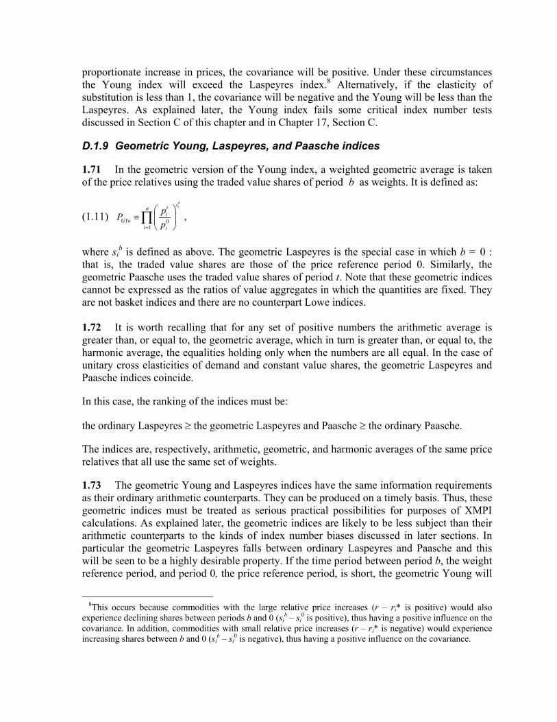
proportionate increase in prices, the covariance will be positive. Under these circumstances the Young index will exceed the Laspeyres index.8 Alternatively, if the elasticity of substitution is less than 1, the covariance will be negative and the Young will be less than the Laspeyres. As explained later, the Young index fails some critical index number tests discussed in Section C of this chapter and in Chapter 17, Section C.
D.1.9 Geometric Young, Laspeyres, and Paasche indices
1.71 In the geometric version of the Young index, a weighted geometric average is taken of the price relatives using the traded value shares of period b as weights. It is defined as:
(1.11) 01
bistn
iGYo
i i
pP
p=
⎛ ⎞≡ ⎜ ⎟
⎝ ⎠∏ ,
where si
b is defined as above. The geometric Laspeyres is the special case in which b = 0 : that is, the traded value shares are those of the price reference period 0. Similarly, the geometric Paasche uses the traded value shares of period t. Note that these geometric indices cannot be expressed as the ratios of value aggregates in which the quantities are fixed. They are not basket indices and there are no counterpart Lowe indices. 1.72 It is worth recalling that for any set of positive numbers the arithmetic average is greater than, or equal to, the geometric average, which in turn is greater than, or equal to, the harmonic average, the equalities holding only when the numbers are all equal. In the case of unitary cross elasticities of demand and constant value shares, the geometric Laspeyres and Paasche indices coincide.
In this case, the ranking of the indices must be:
the ordinary Laspeyres ≥ the geometric Laspeyres and Paasche ≥ the ordinary Paasche.
The indices are, respectively, arithmetic, geometric, and harmonic averages of the same price relatives that all use the same set of weights.
1.73 The geometric Young and Laspeyres indices have the same information requirements as their ordinary arithmetic counterparts. They can be produced on a timely basis. Thus, these geometric indices must be treated as serious practical possibilities for purposes of XMPI calculations. As explained later, the geometric indices are likely to be less subject than their arithmetic counterparts to the kinds of index number biases discussed in later sections. In particular the geometric Laspeyres falls between ordinary Laspeyres and Paasche and this will be seen to be a highly desirable property. If the time period between period b, the weight reference period, and period 0, the price reference period, is short, the geometric Young will
8This occurs because commodities with the large relative price increases (r – ri* is positive) would also
experience declining shares between periods b and 0 (sib – si
0 is positive), thus having a positive influence on the covariance. In addition, commodities with small relative price increases (r – ri* is negative) would experience increasing shares between b and 0 (si
b – si0 is negative), thus having a positive influence on the covariance.
approximate the geometric Laspeyres. The geometric Young is preferred to its arithmetic counterpart. Its main disadvantage may be that, because it is not fixed-basket index, it is not so easy to explain or justify to users. The Lowe index as a fixed basket index is easier to explain in this respect. An objection to geometric means in general used to be that they were difficult to explain to lay users. However, the widespread adoption of the unweighted geometric mean at elementary level for CPIs detracts from this objection.
D.1.10 Symmetric indices
1.74 When the base and current periods are far apart, the index number spread between the numerical values of a Laspeyres and a Paasche price index is liable to be quite large, especially if relative prices have changed a lot (as shown in Appendix 16.1 and illustrated numerically in Chapter 20). Index number spread is a matter of concern to users because, conceptually, there is no good reason to prefer the weights of one period to those of the other. In these circumstances, it seems reasonable to take some kind of symmetric average of the two indices. More generally, it seems intuitive to prefer indices that treat both of the periods symmetrically instead of relying exclusively on the weights of only one of the periods. It will be shown later that this intuition can be backed up by theoretical arguments. There are many possible symmetric indices, but there are three in particular that command much support and are widely used.
1.75 The first is the Fisher price index, PF, defined as the geometric average of the Laspeyres and Paasche indices; that is,
(1.12) F L PP P P≡ × . 1.76 The second is the Walsh price index, PW, a pure price index in which the quantity weights are geometric averages of the quantities in the two periods; that is
(1.13) 0
1
0 0
1
nt ti i i
iW n
ti i i
i
p q qP
p q q
=
=
≡∑
∑.
The averages of the quantities need to be geometric rather than arithmetic for the relative quantities in both periods to be given equal weight. 1.77 The third index is the Törnqvist price index, PT, defined as a geometric average of the price relatives weighted by the average revenue shares in the two periods:
(1.14) ( )0
1
in
tT i i
i
P p pσ
=
=∏ ,
where σi is the arithmetic average of the share of revenue on commodity i in the two periods,
(1.15) 0
2
ti i
is s
σ+
= ,
and where the si are defined as in equation (1.4) and above. The theoretical attractions of these indices become apparent in the following sections on the axiomatic and economic approaches to index numbers.
D.1.11 Fixed-base versus chain indices
Fixed-basket indices
1.78 This topic is examined in Section F of Chapter 16. When a time series of Lowe or Laspeyres indices is calculated using a fixed set of quantities, the quantities become progressively out of date and increasingly irrelevant to the later periods whose prices are being compared. The base period whose quantities are used has to be updated sooner or later, and the new index series linked to the old. Linking is inevitable in the long run.
1.79 In a chain index, each link consists of an index in which each period is compared with the preceding one, the weight and price reference periods being moved forward each period. Any index number formula can be used for the individual links in a chain index. For example, it is possible to have a chain index in which the index for t + 1 on t is a Lowe index defined as ∑ pt+1qt–j / ∑ ptqt–j. The quantities refer to some period that is j periods earlier than the price reference period t. The quantities move forward one period as the price reference period moves forward one period. If j = 0, the chain Lowe becomes a chain Laspeyres, while if j = –1, [that is, t – (–1) = t + 1], it becomes a chain Paasche.
1.80 The XMPIs in some countries are, in fact, annual chain Lowe indices of this general type, the quantities referring to some year, or years, that precedes the price reference period 0 by a fixed period. For example, the 12 monthly indices from January 2005 to January 2006, with January 2005 as the price reference period could be Lowe indices based on price updated trade weights for 2004. The 12 indices from January 2006 to January 2007 are then based on price updated trade weights for 2005; and so on with annual weight updates.
1.81 The trade shares weights lag behind the January price reference period by a fixed interval, moving forward a year each January as the price reference period moves forward one year. Although, for practical reasons, there has to be a time lag between the quantities and the prices when the index is first published, it is possible to retrospectively recalculate the monthly indices, using current period trade value data, or an average of previous and current period data when such data becomes available. In this way, it is possible for the long-run index to be an annually chained monthly index with contemporaneous annual weights. This method is explained in more detail in Chapter 10.
1.82 A chain index between two periods has to be “path dependent.” It must depend on the prices and quantities in all the intervening periods between the first and last periods in the index series. Path dependency can be advantageous or disadvantageous. When there is a gradual economic transition from the first to the last period with smooth trends in relative prices and quantities, chaining will tend to reduce the index number spreads among the
Lowe, Laspeyres, and Paasche indices, thereby making the movements in the index less dependent on the choice of index number formula.
1.83 However, if there are fluctuations in the prices and quantities in the intervening periods, chaining may not only increase the index number spread but also distort the measure of the overall change between the first and last periods. For example, suppose all export prices in the last period return to their initial levels in period 0, which implies that they must have fluctuated in between, a chain Laspeyres XPI does not return to 100. It will be greater than 100. If the cycle is repeated, with all the prices periodically returning to their original levels, a chain Laspeyres index will tend to “drift” further and further above 100 even though there may be no long-term upward trend in the prices. Chaining is therefore not advised when the prices fluctuate widely. When monthly prices are subject to regular and substantial seasonal fluctuations, for example, monthly chaining cannot be recommended. Seasonal fluctuations cause serious problems (see Chapter 23). While a number of countries update their weights annually, the 12 monthly indices within each year are not chain indices but Lowe indices using fixed annual quantities. For some countries, and commodity groups within countries, there may be major fluctuations in export/import value shares and there may be a case for smoothing the weights by taking a rolling average of them over a short run of years. Weights should be updated frequently. Administrative data from customs on weights are less costly than that for CPIs and PPIs. If possible weights should be updated annually, or less frequently as resources permit, but at least every five years. However, for commodity groups with irregular annual patterns, a rolling average over a suitably short number of years is appropriate. Monthly and quarterly updating of weights is not advised, as noted above, especially so for seasonal commodities or commodities with irregular trade.
The Divisia index
1.84 If the prices and quantities are continuous functions of time, it is possible to partition the change in their total value over time into price and quantity components following the method pioneered by Divisia. As shown in Section E of Chapter 16, the Divisia index may be derived mathematically by differentiating value (that is, price times quantity) with respect to time to obtain two components: a relative value-weighted price change and relative value-weighted quantity change. These two components are defined to be price and quantity indices, respectively. The Divisia index is essentially a theoretical index. In practice, prices can be recorded only at discrete intervals even if they vary continuously with time. A chain index may, however, be regarded as a discrete approximation to a Divisia index. The Divisia index itself offers no practical guidance about the kind of index number formula to choose for the individual links in a chain index.
D.2 Axiomatic Approach to Index Numbers
D.2.1 The axioms
1.85 The axiomatic approach to index numbers is explained in Chapter 17. It seeks to decide the most appropriate formula for an index by specifying a number of axioms, or tests, that the index ought to satisfy. It throws light on the properties possessed by different kinds of indices, some of which are by no means intuitively obvious. Indices that fail to satisfy
certain basic or fundamental axioms, or tests, may be rejected completely because they are liable to behave in unacceptable ways. The axiomatic approach is also used to rank indices on the basis of their desirable, and undesirable, properties.
1.86 Twenty axioms or tests (T) are initially considered in Chapter 17. Only a selection of them are given here by way of illustration.
T1—Positivity: The price index and its constituent vectors of prices and quantities should be positive. T3—Identity Test: If the price of every commodity is identical in both periods, then the price index should equal unity, no matter what the quantity vectors are. T5—Proportionality in Current Prices: If all prices in period t are multiplied by the positive number λ, then the new price index should be λ times the old price index; that is, the price index function is (positively) homogeneous of degree one in the components of the period t price vector. T10—Invariance to Changes in the Units of Measurement (commensurability test): The price index does not change if the units in which the commodities are measured are changed. T11—Time Reversal Test: If all the data for the two periods are interchanged, then the resulting price index should equal the reciprocal of the original price index. T12—Quantity Reversal Test: If the quantity vectors for the two periods are interchanged, then the price index remains invariant. T14—Mean Value Test for Prices: The price index lies between the highest and the lowest price relatives. T16—Paasche and Laspeyres Bounding Test: The price index lies between the Laspeyres and Paasche indices. T17—Monotonicity in Current Prices: If the only change is that any period t price is increased, then the price index must increase. 1.87 Some of the axioms or tests can be regarded as more important than others. Indeed, some of the axioms seem so inherently reasonable that it might be assumed that any index number actually in use would satisfy them. For example, test T10, the commensurability test, says that if milk is measured in liters instead of pints, the index must be unchanged. One index that does not satisfy this test is the ratio of the arithmetic means of the prices in the two periods (the Dutot index—discussed in more detail in Chapter 21, Sections C and F).
1.88 Consider, for example, the average price of salt and pepper. Suppose it is decided to change the unit of measurement for pepper from grams to ounces while leaving the units in which salt is measured (for example kilos) unchanged. Because an ounce is equal to 28.35 grams, the absolute value of the price of pepper increases by over 28 times, which effectively
increases the weight of pepper in the Dutot index by over 28 times. When the commodities covered by an index are heterogeneous and measured in different physical units, the value of any index that does not satisfy the commensurability test depends on the purely arbitrary choice of units. Such an index must be unacceptable conceptually. However, when the prices refer to a strictly homogeneous set of commodities that all use the same unit of measurement, the test becomes irrelevant. In practice, commodities may differ in terms of their quality characteristics, and there is a sense in which this variation in quality is similar to variation in the units of measurement. While the quality of individual commodities may not change, the price changes of the higher-price varieties of, say, types of pepper, when aggregated, will be given more emphasis in the calculation.
1.89 Another important test is T11, the time reversal test. In principle, it seems reasonable to require that the same result should be obtained whichever of the two periods is chosen as the price reference period: in other words, whether the change is measured forward in time, forward from 0 to t, or backward in time, from t to 0. The Young index fails this test because an arithmetic average of a set of price relatives is not equal to the reciprocal of the arithmetic average of the reciprocals of the price relatives. This follows from the general algebraic result that the reciprocal of the arithmetic average of a set of numbers is the harmonic average of the reciprocals, not the arithmetic average of the reciprocals. The fact that the conceptually arbitrary decision to measure the change in prices forward from 0 and t gives a different result from measuring backward from t to 0 is seen by many users as a serious disadvantage. The failure of the Young index to satisfy the time reversal test needs to be taken into account by statistical offices.
1.90 Both Laspeyres and Paasche indices fail the time reversal test for the same reasons as the Young index. For example, the formula for a Laspeyres calculated backward from t to 0, PBL, is:
(1.16) 0
1
1
1
nt
i ii
BL Pnt ti i
i
p qP P
p q
=
=
= ≡∑
∑.
1.91 This index is identical with the reciprocal of the (forward) Paasche, not with the reciprocal of the forward Laspeyres. As already noted, the (forward) Paasche tends to register a smaller increase than the (forward) Laspeyres, so that the Laspeyres index cannot satisfy the time reversal test. The Paasche index also fails the time reversal test. 1.92 On the other hand, the Lowe index satisfies the time reversal test provided that the quantities qi
b remain fixed when the price reference period is changed from 0 to t. However, the quantities of a Laspeyres index are those of the price reference period, by definition, and must change whenever the price reference period is changed. The basket for a forward Laspeyres is different from that for the backward Laspeyres, and the Laspeyres fails the time reversal test as a consequence.
1.93 Similarly, the Lowe index is transitive whereas the Laspeyres and Paasche indices are not. Assuming that a Lowe index uses a fixed set of quantities, qi
b, whatever the price reference period, it follows that
PLo0, t = PLo
0, t–k • PLot—k, t
where PLo
0, t is the Lowe index for period t with period 0 as the price reference period. The Lowe index that compares t directly with 0 is the same as that calculated indirectly as a chain index through period t–k. 1.94 If, on the other hand, the Lowe index is defined in such a way that quantities vary with the price reference period, as in the index ∑ pt+1qt–j / ∑ ptqt–j considered earlier, the resulting chain index is not transitive. The chain Laspeyres and chain Paasche indices are special cases of this index.
1.95 In reality, quantities do change and the whole point of chaining is to enable the quantities to be continually updated to take account of the changing trade patterns and universe of commodities. Achieving transitivity by arbitrarily holding the quantities constant, especially over a very long period of time, does not compensate for the potential bias to index numbers introduced by using out of date quantities.
D.2.2 Ranking of indices using the axiomatic approach
1.96 In Section B.6 of Chapter 17 it is shown not only that the Fisher price index satisfies all the 20 axioms initially listed in the chapter but also, more remarkably, that it is the only possible index that can satisfy all 20 axioms. Thus, on the basis of this set of axioms, the Fisher clearly dominates other indices.
1.97 In contrast to Fisher, the other two symmetric indices defined in equations (1.13) and (1.14) above do not emerge too well from the 20 tests. In Section B.7 of Chapter 17, it is shown that the Walsh price index fails four tests whereas the Törnqvist index fails nine tests. Although the Törnqvist index does not perform well on these tests, especially compared with Fisher, it should be remembered that the Törnqvist index and Fisher index may, nevertheless, be expected to approximate each other quite closely when the data follow relatively smooth trends, as shown in Chapter 20.
1.98 The Lowe index with fixed quantities emerges quite well from the axiomatic approach. In particular, in contrast to the Laspeyres, Paasche, and Young indices, it satisfies the time reversal test. As already explained, however, the attractiveness of the Lowe index depends very much on the positioning of period b that supplies the quantity weights, rather than its axiomatic properties.
1.99 One limitation of the axiomatic approach is that the list of axioms itself is inevitably arbitrary to some extent. Some axioms, such as the Paasche and Laspeyres bounding test failed by both Törnqvist and Walsh, could be regarded as contrived and dispensable. In particular many of the test properties have an arithmetic basis, whereas the Törnqvist index is a geometric average. Additional axioms or tests can be envisaged, and indeed two further
axioms are considered below. Another problem with a simple application of the axiomatic approach is that it is not sufficient to know which tests are failed. It is also necessary to know how badly an index fails. Badly failing one major test, such as the commensurability test, might be considered sufficient to rule out an index, whereas failing several minor tests marginally may not be very disadvantageous.
D.2.3 Some further tests
1.100 Consider a further symmetry test. It is reasonable that reversing the roles of prices and quantities in a price index should yield a volume index of the same formula as the price index. A formula that is good enough for a price index should be equally good for a volume index. The factor reversal test requires that the product of such a volume index and the original price index should be identical with the change in the value of the aggregate in question. This test is important if, as stated at the outset of this chapter, price and volume indices are intended to enable changes in the values of aggregates over time to be factored into their price and quantity components in an economically meaningful way. Another remarkable result derived from the axiomatic approach, and given in Section B.6 of Chapter 17, is that the Fisher index is the only price index to satisfy four minimal tests: T1 (positivity), T11 (time reversal), T12 (quantity reversal) and T21 (factor reversal).9 Because the factor reversal test implicitly assumes that the prices and quantities must refer either to period 0 or to period t, it is not relevant to a Lowe index in which three periods are involved, b, 0, and t.
1.101 It was shown earlier that the product of the Laspeyres price (volume) index and the Paasche volume (price) index is identical with the change in the total value of the aggregate in question. Because Laspeyres and Paasche have different functional forms, this implies that they fail the factor reversal test. However, Laspeyres and Paasche indices may be said to satisfy a weak version of the factor reversal test in that dividing the value change by a Laspeyres or Paasche price index does lead to a meaningful volume index, even though its formula is not identical with that of the price index.
1.102 Another test, discussed in Section C.8 of Chapter 17, is the additivity test. A good property for an index is that the changes in the subaggregates add up to the changes in the totals. This is more important from the perspective of volume indices than it is for price indices. Price indices may be used to deflate value changes to obtain implicit volume changes. The results may be presented for subaggregates such as industry or commodity groups. Just as import and export aggregates at current prices are, by definition, obtained simply by summing individual values for import and export transactions or over detailed subaggregate commodity groups, it is reasonable to expect that the changes in the subaggregates of a volume index should add up to the changes in the totals—the additivity test. Volume indices that use a common set of prices to value quantities in both periods must satisfy the additivity test. Similarly, if the Lowe volume index is defined as ∑ pjqt / ∑ pjq0 it is also additive. The Geary-Khamis volume index used to make international comparisons of real consumption and GDP between countries is an example of such a Lowe volume index. It
9See Funke and Voeller (1978, p. 180).
uses an arithmetically weighted average of the prices in the different countries as the common price vector pj to compare the quantities in different countries.
1.103 An alternative solution is to use some average of the prices in two periods to value the quantities. If the volume index is also to satisfy the time reversal test, the average must be symmetrical. The invariance to proportional changes in current prices test (which corresponds to test T7 listed in Chapter 17 except that the roles of prices and quantities are reversed) requires that a volume index depend only on the relative, not the absolute, level of the prices in each period. The Walsh volume index satisfies this test, is additive, and satisfies the time reversal test as well. It emerges as a volume index with some very desirable properties.10
1.104 Although the Fisher index itself is not additive, it is possible to decompose the overall percentage change in a Fisher price, or volume, index into additive components that reflect the percentage change in each price or volume. A similar multiplicative decomposition is possible for a Törnqvist price or volume index.
D.3 Stochastic Approach
1.105 The stochastic approach treats the observed price relatives as if they were a random sample drawn from a defined universe whose mean can be interpreted as the general rate of inflation. However, there can be no single unique rate of inflation. There are many possible universes that can be defined, depending on which particular sets of commodities, industries, or transactions the user is interested in. Clearly, the sample mean depends on the choice of universe from which the sample is drawn. The stochastic approach does not help decide on the choice of universe. It addresses issues such as the appropriate form of average to take and the most efficient way to estimate it from a sample of price relatives, once the universe has been defined.
1.106 The stochastic approach becomes particularly useful when the universe is reduced to a single type of commodity. When there are market imperfections, there may be considerable variation within a country in the prices at which a single commodity is sold by different establishments and also in their movements over time. In practice, statistical offices have to estimate the average price change for a single commodity from a sample of price observations. Important methodological issues are raised, which are discussed in some detail in Chapter 6 on sampling issues and Chapter 21 on elementary indices.
D.3.1 Unweighted stochastic approach
1.107 In Section C.2 of Chapter 17, the unweighted stochastic approach to index number theory is explained. If simple random sampling has been used to collect prices, equal weight may be given to each sampled price relative. Suppose each price relative can be treated as the
10Additivity is a property that is attractive in a national accounts context, where many aggregates are actually
defined by processes of addition and subtraction. It is also useful when comparing national accounts data for different countries using purchasing power parities (PPPs), a type of international price index. (See CPI Manual, International Labour Office, and others, (Geneva, 2004), Annex 4.)
sum of two components: a common inflation rate and a random disturbance with a zero mean. Using least-squares or maximum likelihood estimators, the best estimate of the common inflation rate is the unweighted arithmetic mean of price relatives, an index formula known as the Carli index. This index can be regarded as the unweighted version of the Young index. This index is discussed further in Section I below on elementary price indices.
1.108 If the random component is multiplicative, not additive, the best estimate of the common inflation rate is given by the unweighted geometric mean of price relatives, known as the Jevons index. The Jevons index may be preferred to the Carli on the grounds that it satisfies the time reversal test, whereas the Carli does not. As explained later, this fact may be decisive when deciding on the formula to be used to estimate the elementary indices compiled in the early stages of XMPI calculations.
D.3.2 Weighted stochastic approach
1.109 As explained in Section F of Chapter 17, a weighted stochastic approach can be applied at an aggregative level covering sets of different commodities. Because the commodities may be of differing economic importance, equal weight should not be given to each type of commodity. The commodities may be weighted on the basis of their share in the total traded value of exports or imports, or other transactions, in some period or periods. In this case, the index (or its logarithm) is the expected value of a random sample of price relatives (or their logarithms) with the probability of any individual sampled commodity being selected being proportional to the traded value of that type of commodity in some period or periods. Different indices are obtained depending on which period’s weights are used and whether the price relatives or their logarithms are used.
1.110 Suppose a sample of price relatives is randomly selected, with the probability of selecting any particular type of commodity being proportional to the traded export or import value of that type of commodity in period 0. The expected price change is then the Laspeyres price index for the universe. However, other indices may also be obtained using the weighted stochastic approach. Suppose both periods are treated symmetrically, and the probabilities of selection are made proportional to the arithmetic mean value shares in both periods 0 and t. When these weights are applied to the logarithms of the price relatives, the expected value of the logarithms is the Törnqvist index. From an axiomatic viewpoint, the choice of a symmetric average of the value shares ensures that the time reversal test is satisfied, while the choice of the arithmetic mean, as distinct from some other symmetric average, may be justified on the grounds that the fundamental proportionality in current prices test, T5, is thereby satisfied.
1.111 The examples of the Laspeyres and Törnqvist indices just given show that the stochastic approach in itself does not determine the form of the index number. There are several stochastic indices to choose from, just as there are many possible universes. However, as already noted, the elementary prices from which most aggregate price indices are constructed usually have to be based on samples of prices, and the stochastic approach may provide useful guidance on how best to estimate them.
D.4 Economic Approach
D.4.1 An overview
1.112 The economic approach differs from the previous approaches in an important respect: quantities are no longer assumed to be independent of prices. The behavioral assumptions underlying the economic theory applied to XMPIs depend on whether we take a resident unit’s or non-resident unit’s perspective. In the former case exporters behave to revenue maximize and importers to cost minimize. In the latter, the exports are purchased by cost minimizers and imports are produced by revenue maximisers.
1.113 Consider import and export price indices from a resident unit’s perspective. If, for example, it is assumed that resident institutional units behave as revenue maximizers in supplying exports to a given economic territory, it follows that they would produce more of commodities with above-average price changes. As a result, the revenue shares in period 1 from such commodities will increase, and therefore, their weights. This behavioral assumption about the firm, as it switches production to higher-priced commodities, allows something to be said about what “true” indices should be and the suitability of different index number formulas. For example, the Laspeyres output or supply price index uses fixed period 0 revenue shares to weight its price relatives and ignores the substitution of production toward commodities with higher relative price changes. It will thus understate aggregate price changes—be biased downward against its true index. The Paasche supply price index uses fixed period 1 weights and ignores the initial revenue shares in period 0. It will thus overstate aggregate price changes—be biased upward against its true index.
1.114 Again, taking a resident unit’s perspective, we can observe a like phenomenon in the opposite direction for import price indices, which represent the price change for a resident institutional unit’s uses of commodities supplied to them by the rest of the world. Resident units purchase the rest of the world’s output. If resident institutional units behave as cost minimizers in purchasing the exports from the rest of the world, it follows that they would use less of commodities with above-average price changes compared with period 0. As a result, the cost shares in period 1 of such commodities will decrease, and therefore, their weights. This behavioral assumption about cost minimizing agents, as they switch uses to lower-priced commodities, allows something to be said about what “true” indices should be and the suitability of different index number formulas. For example, the Laspeyres input price index uses fixed period 0 import value shares to weight its price relatives and ignores the substitution of imports away from commodities with higher relative price changes between periods 0 and 1. It will thus overstate aggregate price changes—be biased upward against its true index. The Paasche input price index uses fixed period 1 weights which while representative of period 1 import value shares ignore, for the period 0 to 1 comparison, the initial import value in period 0. It will thus understate aggregate price changes—be biased downward against its true index.
1.115 The nonresident’s approach, the approach primarily used in national accounts, identifies imports as outputs from producers in the rest of the world—the behavioral assumption would be one of revenue maximization by these nonresident producers and the Laspeyres price index would be expected to be biased downward against its true index and
the Paasche price index biased upward against its true index. The nonresident’s approach to exports as inputs to, or uses by, the rest of the world may take cost minimization by economic agents in the rest of the world as its behavioral assumption—Laspeyres would be expected to be biased upwards against its true index and the Paasche index biased downwards, As discussed in Section B above the different perspectives are appropriate for different uses.
Table 1.1, Behavioral assumptions for resident’s and non-resident’s approaches
1.119 The analysis here proceeds mainly from the resident’s perspective. This is for two reasons: First, the treatment from the non-resident’s perspective is well documented in Dridi and Zieschang (2004). Second, the distinguishing feature of the two approaches for the purpose of economic theory is the behavioral assumptions. There are essentially two sets of theory—those from cost minimizing behavioral assumptions and those from revenue maximizing assumptions. As is apparent from Table 1.1, the findings for exports from the resident’s approach applies to those of imports from the non-resident’s approach, and findings for imports from the resident’s approach applies to those of exports from the non-resident’s approach. There is simply no need to replicate the outline of the theory from one perspective given it has been undertaken from the other. As outlined above, the nature of these assumptions affect the results for the direction of the bounds on the theoretical “true” indices. However, the behavioral assumptions, and thus distinction between resident’s and non-resident’s perspectives, do not affect the validity of superlative indices, outlined below, since they are averages of these bounds and it thus does not matter which direction they take.
1.121 The economic approach thus is very powerful, since it identifies a type of bias in Laspeyres and Paasche indices not apparent from other approaches: substitution bias. Laspeyres and Paasche indices ignore the change in weights as producers substitute their production toward, and substitute their uses away from, commodities with above-average price increases. Yet the nature of the bias arises from an assumption about the behavior of producers and other economic units engaged in international trade—that they are revenue maximizers and cost minimizers. Chapter 18 shows that Laspeyres and Paasche indices can under certain conditions act as bounds on a more generally applicable “true” economic theoretic index. The axiomatic approach in Section C led to an index number formula that used an average of the Laspeyres and Paasche indices, and even at this early stage in the discussion, the economic approach seems to provide further support.
1.122 The economic approach also identifies the circumstances under which the conventionally used Laspeyres index is appropriate. This would require, for exports by
resident producers, that the firm does not change its production configuration in response to relative price changes, at least over the short term of the price index comparisons. Economic theory thus argues that the Laspeyres index may be appropriate for industries in which quantities are known not to respond to relative price changes over the period of the price comparisons. But this may be the exception rather than the norm, and the theory points to a requirement for a more generally applicable index number formula, one that also encompasses rigidities in substitution. The economic approach, as shown in Chapter 18, demonstrates that:
• A substitution bias can exist when using Laspeyres and Paasche formulas. The nature of the bias depends on the behavioral assumptions of the firm, which will vary depending on the residency orientation and whether we consider exports or imports.
• The direction of the bias in Laspeyres and Paasche export and import price indices
depends on whether the exports from and imports to a given economic territory are oriented from the nonresident point of view (where exports are uses by the rest of the world and imports are supplies from the rest of the world, the primary approach in the national accounts) or resident point of view (where exports are supplies by residents to the rest of the world and imports are resident’s uses of supply from the rest of the world).
• Laspeyres and Paasche indices act as bounds on their true indices and, under certain
conditions, also are bounds for a more generally applicable true index. • It follows that some symmetric average of these bounds is justified from economic
theory. 1.123 The approach from economic theory is thus first to develop theoretical index number formulas based on what are considered to be reasonable models of economic behavior by the resident unit supplying exports and purchasing imports. This approach is very different from the others considered here. Consider an establishment supplying exports and purchasing imports. A mathematical representation of the production activity—whereby capital and labor conjoin to turn intermediate inputs into outputs—is required for an output index and a representation of the input cost is required for an input index.11 Also, required is an assumption of optimizing behavior (cost minimization or revenue maximization), along with assumptions relating to the form or nature of the mathematical representation of the production/cost function, so that a theoretical index can be derived that is “true” under these conditions. The economic approach then examines practical index number formulas such as Laspeyres, Fisher, and Törnqvist, and considers how they compare with “true” formulas defined under different assumptions. Two theoretical formulations will be examined. Neither can be practically calculated (for reasons that will be explained), but both can be closely approximated. The resident producer’s export price index is supported by the concept of the
11 If our concern was with a model for consumers purchasing imports a mathematical function of the utility derived from purchasing different quantities is required, a utility function; see ILO and others (2004a), Chapter 17.
fixed-input output price index. This index is a ratio of hypothetical revenues over the two periods being compared, say periods 0 and 1, that the revenue-maximizing resident establishment could realize, where the technology and inputs to work with were fixed to be the same for both of the periods. An establishment that, for example, doubles its revenue using a fixed technology and inputs, effectively doubles its prices. The theoretical index is a ratio of revenues, so it incorporates substitution effects as more revenue is obtained as firms substitute toward higher-priced commodities. The theoretical index wishes to have as its period 1 quantities the results of the firm changing the mix of output it produces in response to relative price changes. But there is a dilemma: only price changes should be reflected, and by allowing quantities to change pure price changes would not be measured. So the theoretical index fixes the amount that can be produced by holding the technology and inputs at some constant level. The firm can change its output mix but must use constant inputs and technology. Note that there is a family of theoretical price indices depending on which period’s reference technology and inputs are held constant: fixed period 0 technology and primary inputs, fixed period 1 technology and primary inputs, or some average of the two.
1.124 We can define the conceptual foundation of the resident producer’s import price index as a theoretical fixed-output input price index. This is the ratio of hypothetical intermediate input costs that the cost-minimizing resident establishment must pay in order to produce a set of outputs, again with technology and primary inputs fixed to be the same for the comparison in both periods.
1.125 The key to understanding the economic approach is the appreciation that theoretical index numbers have a strong conceptual basis. As noted above, a family of such index numbers can be derived some of which are based on more restrictive assumptions than others. Actual index number formula can then be appraised in terms of whether they correspond to or approximate theoretical index number formula with good foundations, as considered in more detail below.
D.4.2 Theoretical output price indices
1.126 The theoretical output price index between periods 0 and 1 is the ratio of the maximum revenues that the establishment could attain when faced with period 0 and 1 prices using a fixed, given technology and a fixed set of inputs. While the discussion is phrased in terms of the output and revenue from a producer, our concern hereafter is with the output or revenue of a resident producer for export. We assume such decisions are separable from those for the output to domestic markets. Consider a theoretical index in which period 0 technology and inputs are held constant, the theoretical counterpart to the Laspeyres index. What is required for the numerator of the ratio is to generate what the period 1 quantities would be, holding the production process and inputs constant in period 0 after the change in relative prices from the period 0 technology and inputs. This in turn requires a mechanism to generate these hypothetical period 1 quantities from the fixed period 0 technology and inputs. In the economic approach the technology of a firm or industry is described in terms of a production (possibility) function, which tells us the maximum amount of output(s) that can be produced from a given set of inputs. If the values of all the inputs to a firm or industry were given, the production function would be able to generate all possible combinations of output of commodities from the technology—it would be a mathematical representation of
the technology that converts inputs to outputs. The prevailing relative prices would dictate exactly how much of each commodity is produced. The economic approach to output price indices relies on the assumption of optimizing behavior on the part of producers in competitive, price-taking markets so that they respond to relative price changes. In this approach, while actual prices are considered for both periods, the quantities in each period may not be the observed ones. They are generated from a given period’s production function (with fixed technology) and level of inputs, using assumptions of maximizing behavior and dictated by relative prices, which may be the ones in another period. This is a powerful analytical framework because it allows us to consider, at least in theory, how quantities would respond to different price regimes (say, period 1 prices) under constant (say, period 0) reference technologies and inputs. They are hypothetical quantities that cannot be observed, but are generated in a mathematical model so that their formulation can be compared with real index number formulas based on observable prices and quantities.
1.127 “Pure” price index number formulas (based on observed data) and theoretical price indices both are defined as the ratios of revenues or costs in two periods. However, by definition, while the quantities are fixed in pure price indices, they vary in response to changes in relative prices in theoretical indices. In contrast to the axiomatic approach to index theory, the economic approach recognizes that the quantities produced are actually dependent on the prices. In practice, rational producers may be expected to adjust the relative quantities they produce in response to changes in relative prices. A theoretical set of XMPIs assumes that an institutional unit or establishment seeking to maximize revenues or minimize cost will make the necessary adjustments. The baskets of goods and services in the numerator and denominator of a theoretical XMPIs are not, therefore, exactly the same.
D.4.3 Upper and lower bounds on a theoretical output price index
1.128 The theoretical output price index between periods 0 and 1 is the ratio of revenues in those periods using fixed technology and inputs. Consider an index that held the technology and inputs constant in period 0. The revenue generated in period 0 from period 0 prices using period 0 technology and inputs is what actually happened: the denominator of the theoretical ratio is the observed revenue, assuming the producer was optimizing revenue. The numerator is period 1 prices multiplied by the hypothetical quantities that would have been produced using the same period 0 technology and inputs, had period 1 prices prevailed. It is not, as in the Laspeyres index, period 1 prices multiplied by the actual quantities produced at period 0 prices using period 0 technology and inputs. Both the theoretical and the Laspeyres indices use the same period 0 technology and inputs, but the theoretical index generates quantities from it as if period 1 prices prevailed, whereas the Laspeyres index uses the actual period 0 quantities. In practice, relative prices may change between the two periods, so the quantities generated will be different. Higher revenue could be achieved by substituting, at least marginally, some commodities that have relatively high price changes for some that have relatively low ones. The theoretical index based on period 0 technology and inputs will take account of this and will increase by more than the Laspeyres index. The theoretical index will be at least equal to or greater than the Laspeyres, since the producer has the possibility of, at worst, producing the same set of commodities as in period 0. Being a revenue maximizer, it is assumed the producer will substitute commodities with relatively high price changes—the Laspeyres index thus incurs a “substitution bias.”
1.129 By a similar line of reasoning, it can be shown that when relative prices change, the theoretical output price index based on period 1 technology and inputs will increase by less than the Paasche index. In other words, as shown in Chapter 18, Section D.1, from the resident (producer) exporter’s perspective the Laspeyres index provides a lower bound to its (period 0) theoretical index, and the Paasche an upper bound to its (period 1) theoretical index. Note that these inequalities are in the opposite direction for imports purchased by the resident producer/consumer; the theory and findings for import price indices is given in section D.5 below. 12
1.130 In the national accounts, nonresident orientation, the Laspeyres export price index is an upper bound to the theoretical export price index, while the Paasche is a lower bound. The reason is that exports are a use of goods and services in the nonresident orientation and thus the theoretical index is an input price index and thus the result of cost minimization calculations. In this same case, the Laspeyres import price index is a lower bound to the theoretical import price index, while the Paasche import price index is an upper bound to the theoretical index. The reason is that imports are a supply of goods in the nonresident orientation, and thus the theoretical import price index is an output price index and thus the result of revenue maximization calculations.
1.131 The practical significance of these results stems from the fact that the Laspeyres and Paasche indices can be calculated directly from the observed prices and quantities, whereas the theoretical indices cannot, thus giving some insight into the bias involved in the use of these two formula. Suppose the official objective is to estimate a base period theoretical output price index from the nonresident producer’s perspective as an import price index, MPI, but that a Laspeyres index is calculated instead for practical reasons. One important conclusion to be drawn from this preliminary analysis is that the Laspeyres MPI may be expected to have a downward bias. Similarly, a series of upwards biased Paasche MPIs from a nonresident producer’s perspective used to deflate a series of import values at current prices generates a volume series of constant price import values (Laspeyres volume index), which in turn will also suffer from a downward bias. The approach informs us that (for both the resident’s and nonresident’s perspective) there are two equally valid theoretical economic price indices, and that the bounds, while useful, only show how Laspeyres and Paasche indices compare with their own theoretical counterparts. What we require are two-sided bounds on the theoretically justified index.
D.4.4 Estimating theoretical output indices by superlative indices
1.132 The next step is to establish whether there are special conditions under which it may be possible to exactly measure theoretical XMPIs. In Section D.2 of Chapter 18 theoretical indices based on weighted “averages” of the period 0 and period 1 technology and similarly weighted averages of the period 0 and 1 inputs are considered. These theoretical indices deal adequately with substitution effects; that is, when, for example, a resident producer’s
12 Importers wish to minimize costs and purchase more of commodities with below average price increases. A
Laspeyres import price index thus overstates its true index by not reflecting the shift in quantities to lower prices commodities. Similarly a Paasche import price index understates its true index.
(output) export price increases, the producer’s supply increases, holding inputs and the technology constant. Such theoretical indices are argued to generally fall between the Laspeyres (lower bound) and Paasche (upper bound) indices. The Fisher index, as the geometric mean of the Laspeyres and Paasche indices, is the only symmetric average of Laspeyres and Paasche that satisfies the time reversal test. Thus, economic theory was used to justify Laspeyres and Paasche bounds, and axiomatic principles led to the Fisher price index as the best symmetric average of these bounds.
1.133 In Section D.3 of Chapter 18 the case for the Törnqvist index number formula is presented. It is assumed (for an resident’s output index) that the revenue function takes a specific mathematical form: a translogarithmic function. If the price coefficients of this translog form are equal across the two periods being compared, then the geometric mean of the economic output price index that uses period 0 technology and the period 0 input vector, and the economic output price index that uses period 1 technology and the period 1 input vector, are exactly equal to the Törnqvist output price index. The assumptions required for this result are weaker than other subsequent assumptions; in particular, there is no requirement that the technologies exhibit constant returns to scale in either period. The ability to relate an actual index number formula (Törnqvist) to a specific functional form (translog) for the production technology is a powerful analytical device. Statisticians using particular index number formulas are in fact replicating particular mathematical descriptions of production technologies. A good formula should not correspond to a restrictive functional form for the production technology.
1.134 Diewert (1976) described an index number formula to be superlative if it is equal to a theoretical price index whose functional form is flexible—it can approximate an arbitrary technology to the second order. That is, the technology by which inputs are converted into output quantities and revenues is described in a manner that is likely to be realistic of a wide range of forms. Relating a class of index number formulas to technologies represented by flexible functional forms is another powerful finding, since it gives credence to this class of index number formulas. Note also that the translog functional form is an example of a flexible functional form, so the Törnqvist output price index number formula is superlative.
1.135 In Section E.3 of Chapter 18 the Fisher index is revisited from a purely economic approach. An additional assumption is invoked, that outputs are homogeneously separable from other commodities in the production function: if the input quantities vary, the output quantities vary with them, so that the new output quantities are a uniform expansion of the old output quantities. It is shown that a homogeneous quadratic production or utility function is flexible and corresponds to the Fisher index. The Fisher output price index is therefore also superlative. This is one of the more famous results in index number theory. Although it is generally agreed that it is not plausible to assume that a production technology would have this particular functional form, this result does at least suggest that, in general, the Fisher index is likely to provide a close approximation to the underlying unknown theoretical XMPI—and certainly a much closer approximation than either the Laspeyres or the Paasche indices can yield on their own.
1.136 This intuition is corroborated by the following line of reasoning. Diewert (1976) noted that a homogeneous quadratic is a flexible functional form that can provide a second-
order approximation to other twice-differentiable functions around the same point. He then described an index number formula that is exactly equal to a theoretical one based on the underlying aggregator function as superlative when that functional form is also flexible—for example, a homogeneous quadratic. The derivation of these results, and further explanation, are given in detail in Sections E.1-3 of Chapter 18. In contrast to the theoretical index itself, a superlative index is an actual index number that can be calculated. The practical significance of these results is that they provide a theoretical justification for expecting a superlative index to provide a fairly close approximation to the unknown underlying theoretical index in a wide range of circumstances.
Superlative indices as symmetric indices
1.137 The Fisher index is not the only example of a superlative index. In fact, there is a whole family of superlative indices. It is shown in Section E.4 of Chapter 18 that any quadratic mean of order r is a superlative index for each value of r ≠ 0. A quadratic mean of order r price index Pr is defined as follows:
(1.17)
2
00
1
20
1
rtnir i
i irr
nt ir i t
i i
psp
Ppsp
=
=
⎛ ⎞⎜ ⎟⎝ ⎠≡⎛ ⎞⎜ ⎟⎝ ⎠
∑
∑,
where si0 and si
t are defined as in equation (1.4) above. 1.138 The symmetry of the numerator and denominator of equation (1.17) should be noted. A distinctive feature of equation (1.17) is that it treats the price changes and value shares in both periods symmetrically whatever value is assigned to the parameter r. Three special cases are of interest:
• When r = 2, equation (1.17) reduces to the Fisher price index; • When r = 1, it is equivalent to the Walsh price index; • In the limit as r → 0, it equals the Törnqvist index. 1.139 These indices were introduced earlier as examples of indices that treat the information available in both periods symmetrically. Each was originally proposed long before the concept of a superlative index was developed.
Choice of superlative index
1.140 Section E.5 of Chapter 18 addresses the question of which superlative formula to choose in practice. Because each may be expected to approximate to the same underlying theoretical output index, it may be inferred that they ought also to approximate to each other. That they are all symmetric indices reinforces this conclusion. These conjectures tend to be borne out in practice by numerical calculations. It seems that the numerical values of the different superlative indices tend to be very close to each other, but only so long as the value of the parameter r does not lie far outside the range 0 to 2. However, in principle, there is no
limit on the value of the parameter r, and in Section E.4 of Chapter 18, it has shown that as the value of r becomes progressively larger, the formula tends to assign increasing weight to the extreme price relatives and the resulting superlative indices may diverge significantly from each other. Only when the absolute value of r is very small, as in the case of the three commonly used superlative indices—Fisher, Walsh, and Törnqvist—is the choice of superlative index unimportant.
1.141 Both the Fisher and the Walsh indices date back nearly a century. The Fisher index owes its popularity to the axiomatic, or test, approach, which Fisher (1922) himself was instrumental in developing. As shown above, it appears to dominate other indices from an axiomatic viewpoint. That it is also a superlative index whose use can be justified on grounds of economic theory suggests that, from a theoretical point of view, it may be impossible to improve on the Fisher index for XMPI purposes.
1.142 However, the Walsh index has the attraction of being not merely a superlative index, but also a conceptually simple pure price index based on a fixed basket of goods and services. That the Walsh index is both a superlative and a pure index throws light on the interrelationships between the theoretical output price index and pure price indices. The distinctive feature of a Walsh index is not just that the basket of goods and services is a simple (geometric) average of the quantities in each of the two periods; by being a geometric average, it also assigns equal importance to the relative, as distinct from the absolute, quantities. Such an index clearly treats both periods symmetrically.13 Pure price indices do not have to diverge from the theoretical output price index and are not inherently biased as estimators of the theoretical index. Bias is only likely to arise when the relative quantities used in a pure price index favor one of the periods at the expense of the other, as in a Laspeyres or Paasche index.
Representativity bias
1.143 That the Walsh index is a Lowe index that is also superlative suggests that the bias in other Lowe indices depends on the extent to which their quantities deviate from those in the Walsh basket. This can be viewed from another angle.
1.144 Because the quantities in the Walsh basket are geometric averages of the quantities in the two periods, equal importance is assigned to the relative, as distinct from the absolute, quantities in both periods. The Walsh basket may therefore be regarded as being the basket that is most representative of both periods.14 If equal importance is attached to the production patterns in the two periods, the optimal basket for a Lowe index ought to be the most representative basket. The Walsh index then becomes the conceptually preferred target index for a Lowe index.
13The Marshall-Edgeworth index (see Chapter 15) uses a simple arithmetic average of the quantities, but the
resulting basket will be dominated by the quantities for one or other of the periods if the quantities are larger, on average, in one period than the other. The Marshall-Edgeworth is not a superlative index.
14The Walsh basket is the one that minimizes the sum of the squares of the logarithmic deviations between the quantities in the two actual baskets and those in the index basket.
1.145 Suppose that period b, whose quantities are actually used in the Lowe index, lies midway between 0 and t. In this case, assuming fairly smooth trends in the relative quantities, the actual basket in period b is likely to approximate the most representative basket. Conversely, the farther away that period b is from the midpoint between 0 and t, the more the relative quantities of b are likely to diverge from those in the most representative basket. In this case, the Lowe index between periods 0 and t that uses period b quantities is likely to exceed the Lowe index that uses the most representative quantities by an amount that becomes progressively larger the farther back in time period b is positioned. The excess constitutes “bias” if the latter index is target the index. The bias can be attributed to the fact that the period b quantities tend to become increasingly unrepresentative of a comparison between 0 and t the farther back period b is positioned. The underlying economic factors responsible are, of course, exactly the same as those that give rise to bias when the target index is the economic index. Thus, certain kinds of indices can be regarded as biased without invoking the concept of an economic index. Conversely, the same kinds of indices that tend to emerge as being preferred, whether or not the objective is to estimate an economic index.
1.146 If interest is focused on short-term price movements, the target index is an index between consecutive time periods t and t + 1. In this case, the most representative basket has to move forward one period as the index moves forward. Choosing the most representative basket implies chaining. Similarly, chaining is also implied for the target economic index t and t + 1. In practice, the universe of commodities is continually changing as well. As the most representative basket moves forward, it is possible to update the set of commodities covered as well as take account of changes in the relative quantities of commodities that were covered previously.
Data requirements and calculation issues
1.147 Because superlative indices require price and traded share value data for both periods and such share data may not be available for the current period, it may not be feasible to calculate superlative XMPIs, at least at the time XMPIs are first published. In practice, it may be necessary for the official index to be a Laspeyres-type index, such as the Lowe or Young. To the extent that trade share data are available on an annual basis, from customs and/or establishment surveys, annual chain Laspeyres-type indices could be produced initially. The advantage of the annual updating is that chaining helps to reduce the spread between the Laspeyres and Paasche indices. Chained indices are highly desirable not only because they reduce spread, but they facilitate the incorporation of new commodities into the index and the dropping of old ones. However, in the course of time more share data may become available, enabling chained superlative XMPIs to be calculated subsequently. Some statistical offices may find it useful to do so, without necessarily revising the original official index. Comparing movements in the official XMPIs with those in a subsequently calculated chained superlative version may be helpful in evaluating and interpreting movements in the official XMPI. It may be that value data can be collected from establishments alongside price data or some customs data with little time lag, and this is to be encouraged so that Fisher XMPI indices may be calculated in real time for at least some commodity sectors.
1.148 Section E.6 of Chapter 18 notes that, in practice, XMPIs are usually calculated in stages (see Chapters 10 and 21) and addresses the question of whether indices calculated this
way are consistent in aggregation—that is, have the same values whether calculated in a single operation or in two stages. The Laspeyres index is shown to be exactly consistent, but superlative indices are not. However, the widely used Fisher and Törnqvist indices are shown to be approximately consistent.
D.4.5 Allowing for substitution
1.149 One further index proposed recently, the Lloyd-Moulton index, PLM, defined as follows:
(1.18)
11 1
00
11
tni
LM ii i
pP s
p
σ σ
σ− −
=
⎧ ⎫⎛ ⎞⎪ ⎪≡ ≠⎨ ⎬⎜ ⎟⎝ ⎠⎪ ⎪⎩ ⎭
∑
1.150 The parameter σ, which must be nonpositive for the price index of the nonresident supply of imports, is the elasticity of substitution between the commodities covered. It reflects the extent to which, on average, the various commodities are believed to be substitutes for each other. The advantage of this index is that it may be expected to be free of substitution bias to a reasonable degree of approximation, while requiring no more data, except for an estimate of the parameter σ, than the Laspeyres index. It is therefore a practical possibility for XMPI calculation, even for the most recent periods. However, it may be difficult to obtain a satisfactory, acceptable estimate of the numerical value of the elasticity of substitution, the parameter used in the formula. D.5 Intermediate input price indices
1.151 Having considered the theory and appropriate formula for output export price indices, Chapter 18 turns to input import price indices (Section F). It is implicit in the description of the export price index as an output one and the import price index as an input one that the resident’s perspective is being taken here, but it is apparent from the preceding discussion in section D.4.1 that a nonresident’s perspective reverses the Laspeyres bounds. It is also apparent from the discussion in sections D.4.4 that the Fisher superlative index, as a symmetric average of Laspeyres and Paasche, will be unaffected by the direction of the bounds and thus whether a resident’s or nonresident’s perspective is taken.
1.152 The behavioral assumption behind the theory of the output export price index is one of producers maximizing a revenue function. An input import price index for producers is concerned with the price changes of intermediate inputs, and the corresponding behavioral assumption is the minimization of a conditional cost function. The producer is held to minimize the cost of intermediate inputs of imported goods and services in order to produce a set of outputs, given a set of intermediate import inputs prices, and given that the primary inputs and technology used on the imported inputs are fixed. Of course cost minimizing decisions regarding intermediate inputs are based on both domestically supplied and imported inputs however we assume that they are separable and, hereafter, inputs refers to imported ones. The primary inputs and technology are assumed to be fixed so that hypothetical input quantities can be generated from a fixed setup that allows the input quantities in period 1 to reflect the producer buying more of those inputs that have become
cheaper. Theoretical intermediate input import price indices are defined as ratios of hypothetical intermediate input import costs that the cost-minimizing producer must pay in order to produce a fixed set of outputs from technology and primary inputs fixed to be the same for the comparison in both periods. As was the case with the theory of the output export price index, theoretical input import indices can be derived on the basis of either fixed period 0 technology and primary inputs, or fixed period 1 technology and primary inputs, or some average of the two. The observable Laspeyres index of intermediate input import prices is shown to be an upper bound to the theoretical intermediate input import price index based on period 0 technology and inputs. The observable Paasche index of intermediate input import prices is a lower bound to its theoretical intermediate input import price index based on period 1 fixed technology and inputs. Note that these inequalities are the reverse of the findings for the output export price index, but that they are analogous to their counterparts in the CPI for the theory of the true cost-of-living index, which is also based on an expenditure (cost) minimization problem. Thus the same findings for input import price indices applies to consumers purchasing imported goods and services.
1.153 Following the analysis for the output export price index, a family of intermediate input import price indices can be shown to exist based on an average of period 0 and period 1 technologies and inputs leading to the result that Laspeyres (upper) and Paasche (lower) indices are bounds on a reasonable theoretical input import index. A symmetric mean of the two bounds is argued to be applicable given that Laspeyres and Paasche indices are equally justifiable, with the Fisher index having support on axiomatic grounds. If the conditional intermediate input import cost function takes the form of a translog technology, the theoretical intermediate input import price index is exactly given by a Törnqvist index, which is superlative. If separability is invoked, Fisher and Walsh indices are also shown to be superlative, and the three indices closely approximate each other.
E. Transfer Prices
1.154 When there is an international transaction between say two divisions of a multinational enterprise that has establishments in two or more countries, then the value of the transaction to the exporting division will be equal to the value of the transaction for the importing division. Thus when the multinational enterprise works out its profits worldwide for the period when the transaction took place, the export value will equal the import value and hence will cancel out, leaving the company’s overall profits unchanged, no matter what price it chose to value the transaction. The price chosen to value the transaction is called a transfer price. Hence, at first glance, it appears that the multinational firm could choose the transfer price for the transaction to be practically anything. However, in a world where there are taxes on international transactions and where the rates of business income taxation differ across countries, the situation is actually worse: the multinational will have definite financial incentives to choose strategically the transfer price to minimize the amount of taxation paid to both jurisdictions. It is this element of strategic choice that casts doubt on the usefulness of simply collecting transfer prices for enterprises as if they were ordinary prices between unrelated parties. 1.155 Strategically chosen transfer prices will generally be very different from economic transfer prices (based on opportunity costs) that would be suitable for an import or export
price index. Since international trade between affiliated units is somewhere in the neighborhood of 30 to 40 percent of world trade, it can be seen that this problem of determining appropriate transfer prices is a serious one. 1.156 Chapter 19 discusses the issues related to transfer prices and offers solutions. The best alternative to the firm’s listed transfer price are internal comparable prices for the two periods compared; that is, the average price paid to (for an imported commodity) or received from (for an exported commodity) unaffiliated firms for the same commodity during the reference period, if such unaffiliated purchases or sales exist. If there are no such unaffiliated purchases or sales, then the use of externally referenced comparable prices is recommended, that is, the price change of the commodity on a recognized exchange that trades in the commodity if such an exchange exists. If no such exchange exists, then attempting to find an external comparable price change based on transactions between unaffiliated traders is recommended. These three methods all focus on the price change of the same commodity traded by different firms. Where this is impossible, downstream prices, or potentially upstream prices can be explored to see whether an economically acceptable price can be found. Finally, if there are no internal or external comparable prices, at the same or different levels of the value chain, the international price index should use the multinational’s stated transfer price.. XMPIs are used to deflate value aggregates in the national accounts so it follows that the (transfer) prices used to compile the price index should match those used in the value aggregates. Price index compilers will need to discuss such issues within their national accounts counterparts.
F. Illustrative Numerical Data
1.157 Chapter 20 presents numerical examples using an artificial data set. The purpose is not to illustrate the methods of calculation as such, but rather to demonstrate how different index number formulas can yield very different numerical results. Hypothetical but economically plausible prices, quantities, and revenues are given for six commodities over five periods of time. In general, differences between the different formulas tend to increase with the variance of the price relatives. They also depend on the extent to which the prices follow smooth trends or fluctuate.
1.158 The numerical results are striking. For example, the Laspeyres index over the five periods registers an increase of 49 percent while the Paasche only rises 19 percent. The two commonly used superlative indices, Törnqvist and Fisher, register increases of 40 percent and 33 percent, respectively, an index number spread of only 7 points compared with the 30 point gap between the Laspeyres and Paasche. When the indices are chained, the chain Laspeyres and Paasche register increases of 47 percent and 28 percent, respectively, reducing the gap between the two indices from 30 to 19 points. The chained Törnqvist and Fisher register increases of 37.7 percent and 37.1, percent respectively. These results show that the choice of index formula and method is crucial.
1.159 Chapter 15 showed how the nominal values of, and thus price indices for, exports and imports fitted into the 1993 System of National Accounts. Particular emphasis was given to the role of price indices as deflators for estimating volume changes in gross domestic product
(GDP) by the expenditure approach. Chapter 20 also outline how price indices for exports and imports can be defined and reconciled from the expenditure and production approaches to estimating GDP. Indeed the illustrative data used to outline and demonstrate differences in the results from different index number formulas are applied not only to export and import price indices, but also to price indices for the constituent aggregates of GDP from both the expenditure and production approaches. The implications for the resident’s and nonresident’s perspectives to price and volume measurement are outlined.
G. Choice of Index Formula
1.19
1.20
1.21 The index theory developed in Chapters 15 to 17 demonstrates that the Fisher and the Törnqvist are equally good alternatives. Indeed, the Fisher may be preferred to Walsh on axiomatic grounds, given that the two indices will tend to give almost identical results for comparisons between successive time periods.
As already noted, for practical reasons the PPI is often calculated as a time series of Laspeyres indices based on some earlier period 0. In this case, the published index between t-1 and t may actually be the monthly change version of the Laspeyres index given in 1.4 above. Given that some substitution effect is operative, which seems extremely likely on both theoretic and empirical grounds, it may be inferred, by reasoning along lines explained in Chapter 15, that the monthly change Laspeyres index will tend to be less than the Walsh index between t-1 and t. If the PPI is intended to measure producer inflation, therefore, the monthly change Laspeyres could have a downward bias, a bias that will tend to get worse as the current period for the Laspeyres index moves further away from the base period. This is the kind of conclusion that emerges from the index theory presented in Chapters 15 and 16. It is a conclusion with considerable policy and financial implications. It also has practical implications as it provides an argument for rebasing and updating a Laspeyres index as often as resources permit, perhaps on an annual basis as many countries are now doing. 1.22
1.23
1.24
1.160 By drawing upon the index number theory surveyed in Chapters 15 to 19 it is possible to decide on the type of index number in any given set of circumstances. However, there is little point in asking what is the best index number formula for XMPIs. The question is too vague. A precise answer requires a precise question. For example, suppose that the principal concern of most users of XPIs is to have the best measure of the current rate of factory gate inflation for exports. The precise question can then be posed: what is the best index number to use to measure the change between periods t-1 and t in the prices of the producer goods and services leaving the factory between periods t-1 and t for export? If the objective of the
XPI is to measure the current rate of change in revenues for a fixed, given technology and set of inputs, to be used for resident export output deflation, this translates into asking what is the best estimate of the change in export producer output prices. The theory elaborated in Chapter 18 shows that the best estimate will be provided by a superlative index. The three commonly used superlative indices are Fisher, Törnqvist, and Walsh. All produce similar answers under small to moderately large changes in prices and quantities, as all approximate one another to the second order of smalls..
1.161 The question itself determines both the coverage of the index and the system of weighting. The establishments in question have to be those of the country in question and not, say, those of some foreign country. Similarly, the question refers to exporting establishments in periods t-1 and t, not to establishments five or ten years earlier. Sets of establishments five or ten years apart are not all the same and their inputs and production technologies change over time.
1.162 As the question specifies goods and services exported in periods t-1 and t, the basket of goods and services used should include all the quantities exported by the establishments in periods t-1 and t, and only those quantities. One index that meets these requirements is a pure price index that uses a basket consisting of the total quantities produced in both periods t-1 and t. This is equivalent to an index that uses a simple arithmetic mean of the quantities in the two periods, an index known as the Edgeworth-Marshall index. However, this index has a slight disadvantage in that if export production is growing, the index gives rather more weight to the quantities produced in period t than those in t-1. It does not treat both periods symmetrically. It fails Tests T.7 and T.8 listed in Chapter 17 on the axiomatic approach, the Invariance to Proportional Changes in Quantities Tests. However, if the arithmetic mean quantities are replaced by the geometric mean quantities, as in the Walsh index, both tests are satisfied. This ensures that the index attaches equal importance to the patterns of production, as measured by relative quantities produced in both t-1 and t.
1.163 The Walsh index therefore emerges as the pure price index that meets all the requirements. It takes account of every single product produced in the two periods. It utilizes all the quantities produced in both periods, and only those quantities. It gives equal weight to the patterns of production in both periods. In practice, it may not be feasible to calculate a Walsh index, but it can be used as the standard by which to evaluate other indices.
1.164 The index theory developed in Chapters 15 to 17 demonstrates that the Fisher and the Törnqvist are equally good alternatives. Indeed, the Fisher may be preferred to Walsh on axiomatic grounds, given that the two indices will tend to give almost identical results for comparisons between successive time periods.
1.165 As already noted, for practical reasons XMPIs often are calculated as a time series of Lowe indices based not even on period t-1 quantities, but on some much earlier period b. A Laspeyres index based on period t-1 quantities between t – 1 and t will be subject to substitution bias. We can infer, then, by reasoning along lines explained in Chapter 16, that the monthly-change Laspeyres resident’s output export price index will tend to be less than the Walsh output export price index. If the XMPIs are intended to measure inflation, therefore, the monthly change Laspeyres export price index could have a downwards bias.
But the bias will tend to get worse as the current period for the Laspeyres index moves further away from the base period: in our case the further period b precedes t-1, which for some countries can be a few years. This is the kind of conclusion that emerges from the index theory presented in Chapters 16 and 18. It is a conclusion with considerable policy and financial implications. It also has practical implications because it provides an argument for rebasing and updating a Lowe index as often as resources permit, preferably on an annual basis as many countries are now doing.
H. Elementary Price Indices
1.166 As explained in Chapters 10 and 21, the calculation of XMPIs typically proceeds in two or more stages. In the first stage, elementary price indices are estimated for the elementary aggregates of an XPI or an MPI. In the second stage, these elementary indices are combined to obtain higher-level indices using the elementary aggregate indices with export or import trade weights. An elementary aggregate consists of the traded values for a small and relatively homogeneous set of commodities defined within the commodity classification used in international trade. Samples of prices are collected within each elementary aggregate, so that elementary aggregates serve as strata for sampling purposes. There are two main sources of data for these prices. First, is data derived from customs documentation: the values of, for example, exports for a detailed classification group within the Harmonized System, are aggregated in a given month and divided by the corresponding aggregate quantities to form a unit value. A similarly defined unit value for the next month is defined and the price change for goods in this classification proxied by the unit value index change. Each unit value index, derived for a detailed commodity classification, has a weight attached to it for aggregation to a higher level of classification. It may be that the unit values compared within the detailed classification are further refined and stratified to relate say to a single country of export, but the principle remains the same. The aggregation of transactions within the unit value indices benefit from quantity information and while it is usual to define the elementary level indices as being unweighted, this is not strictly so for unit value indices. However, unit value indices do relate to aggregation that is practically at the lowest level of aggregation for the period in question. The index number properties of unit value indices and their suitability as proxies to represent price changes has been the subject of Section B and, in detail, Chapter 2. These lower level unit value indices can only be meaningfully defined for strictly homogeneous goods and any change in their quality composition between the months compares renders them subject to errors. Given that the use of unit value indices at the lower level has been discussed, this chapter addresses itself to the second data source for elementary aggregate price indices, that from establishment surveys.
1.167 Data on the traded value shares, or quantities, of the representative goods and services whose prices are monitored and compared each period may not be available within an elementary aggregate from an establishment survey. Since it has been shown that it is theoretically appropriate to use superlative formulas, data on trade value shares should be collected alongside those on prices whenever possible. Given that this may not be possible in order to meet the timeliness requirements of users—that is, there are no quantity or value share weights—most of the index number theory outlined in the previous sections is not applicable. An elementary price index is a more primitive concept that relies on price data only. It is something calculated when there is no explicit or implicit quantity or value data
available for weights. Implicit quantity or value data may arise from a sampling design whereby the selection of commodities is with probability proportionate to quantities or sales value.
1.168 The question of what is the most appropriate formula to use to estimate an elementary price index is considered in Chapter 21. This topic was comparatively neglected until a number of papers in the 1990s provided much clearer insights into the properties of elementary indices and their relative strengths and weaknesses. Since the elementary indices are the building blocks from which XMPIs are constructed, the quality of a set of XMPIs depends heavily on them.
1.169 As explained in Chapter 7, compilers have to select representative and well defined items within an elementary aggregate and then collect a sample of prices for each of the representative items, usually from a sample of different establishments. The individual items whose prices are actually collected are described as the sampled items. Their prices are collected over a succession of time periods. An elementary price index is, therefore, typically calculated from two sets of matched price observations. It is assumed in this section that there are no missing observations and no changes in the quality of the items sampled, so that the two sets of prices are perfectly matched. The treatment of new and disappearing items, and of quality change, is a separate and complex issue that is discussed in detail in Chapters 8, 9, and 22 of the Manual.
1.170 The price quotes for the elementary aggregate indices are assumed to be collected from price surveys of establishments and relate to matched specified commodities whose quality characteristics are well specified.
H.1 Heterogeneity of commodities within an elementary aggregate
1.171 If a number of different representative items are selected for pricing, the set of items within an elementary aggregate cannot be homogeneous. Even a single representative item may not be completely homogeneous, depending upon how tightly it is specified. The degree of heterogeneity of the sampled items must be explicitly taken into account in the calculation of an elementary index.
1.172 When the quantities are not homogeneous, they cannot be meaningfully added from an economic viewpoint, and their prices should not be averaged. Consider again the example of salt and pepper, which might be representative items within an elementary aggregate. Pepper is an expensive spice sold in very small quantities such as ounces or grams, whereas salt is relatively cheap and sold in much larger quantities, such as pounds or kilos. A simple arithmetic average of, say, the price of a gram of pepper and the price of a kilo of salt is an arbitrary statistic whose value depends largely on the choice of the quantity units. Choosing the same physical unit of quantity, such as a kilo, for both does not resolve the problem, because both the average price and the change in the average price would be completely dominated by the more expensive commodity, pepper, even though exporters may obtain more revenue from salt. In general, arithmetic averages of prices should be taken only when the corresponding quantities are homogeneous and can be meaningfully added.
H.2 Weighting
1.173 As already noted, it is assumed in this section that there are no quantities or trade share value data available to weight the prices, or the price relatives, used to calculate an elementary index. If they were available, it would usually be preferable to use them to decompose the elementary aggregate into smaller and more homogeneous aggregates.
1.174 However, some system of weighting may have been implicitly introduced into the selection of the sampled items by the sample design used. For example, the establishments from which the prices are collected may have been selected using probabilities of selection that are proportional to their sales or some other variable.
H.3 Interrelationships between different elementary index formulas
1.175 Valuable insights into the properties of various formulas that might be used for elementary price indices may be gained by examining the numerical relationships between them, as explained in Section D of Chapter 21. There are two basic options for an elementary index:
• To average the price relatives—that is, the ratios of the matched prices; • To calculate the ratio of average prices in each period. 1.176 It is worth recalling that for any set of positive numbers the arithmetic average is greater than or equal to the geometric average, which in turn is greater than or equal to the harmonic average, the equalities holding only when the numbers are all equal. Using these three types of average, the ranking of the results obtained by the second method are predictable. It should also be noted that the ratio of geometric averages is identical with the geometric average of the ratios. The two methods give the same results when geometric averages are used.
1.177 As explained in Section C of Chapter 21, there are several elementary price indices that might possibly be used. Using the first of the above options, three possible elementary price indices are:
• The arithmetic average of the price relatives, known as the Carli index, or PC; the Carli is the unweighted version of the Young index.
• The geometric average of the price relatives, known as the Jevons index, or PJ; the Jevons is the unweighted version of the geometric Young index.
• The harmonic average of the price relatives, or PH. As just noted, PC ≥ PJ ≥. PH. Using the second of the options, three possible indices are:
• The ratio of the arithmetic average prices, known as the Dutot index, or PD; • The ratio of the geometric averages, again the Jevons index, or PJ; • The ratio of the harmonic averages, or RH.
The ranking of ratios of different kinds of average are not predictable. For example, the Dutot, PD, could be greater or less than the Jevons, PJ. 1.178 The Dutot index can also be expressed as a weighted average of the price relatives, in which the prices of period 0 serve as the weights:
(1.19)
00
11
0 0
1 1
tnnit
iii ii
D n n
i ii i
ppp n pP
p n p
==
= =
⎛ ⎞⎜ ⎟⎝ ⎠≡ =
∑∑
∑ ∑.
1.179 As compared with the Carli, which is a simple average of the price relatives, the Dutot index gives more weight to the price relatives for the items with high prices in period 0. However, it is difficult to provide an economic rationale for this kind of weighting. Prices are not revenues or expenditures. If the items are homogeneous, very few quantities are likely to be purchased at high prices if the same items can be purchased at low prices. If the items are heterogeneous, the Dutot should not be used anyway, since the quantities are not commensurate and not additive. 1.180 Noting that PC ≥ PJ ≥. PH, it is shown in Section D of Chapter 21 that the gaps between these indices widen as the variance of the price relatives increases. The choice of formula becomes more important the greater the diversity of the price movements. Moreover, both PD and PJ can be expected to lie approximately halfway between PC and PH. While it is useful to establish the interrelationships between the various indices, they do not actually help decide which index to choose. However, because the differences between the various formulas tend to increase with the dispersion of the price relatives, it is clearly desirable to define the elementary aggregates in such a way as to try to minimize the variation in the price movements within each aggregate. The less variation, the less difference the choice of index formula makes. Since the elementary aggregates also serve as strata for sampling purposes, minimizing the variance in the price relatives within the strata will also reduce the sampling error.
H.4 Axiomatic approach to elementary indices
1.181 One way to decide between the various elementary indices is to exploit the axiomatic approach outlined earlier. A number of tests are applied to the elementary indices in Section E of Chapter 21.
1.182 The Jevons index, PJ, satisfies all the selected tests. It dominates the other indices in the way that the Fisher tends to dominate other indices at an aggregative level. The Dutot index, PD, fails only one, the commensurability test. This failure can be critical, however. It reflects the point made earlier that when the quantities are not economically commensurate, their prices should not be averaged. However, PD performs well when the sampled items are homogeneous. The key issue for the Dutot index is, therefore, how heterogeneous are the
items within the elementary aggregate. If the items are not sufficiently homogeneous for their quantities to be additive, the Dutot index should not be used.
1.183 The Carli index, PC, is widely used, but the axiomatic approach shows that it has some undesirable properties. In particular, as the unweighted version of the Young index, it fails the product reversal, the time reversal, and the transitivity tests. These are serious disadvantages, especially when month-to-month indices are chained. A consensus has emerged that the Carli may be unsuitable because it is liable to have a significant upward bias. This is illustrated by numerical example in Chapter 10. Its use is not sanctioned for the Harmonized Indices of Consumer Prices used within the European Union. Conversely, the harmonic average of the price relatives, PH, is liable to have an equally significant downward bias, although it does not seem to be used in practice anyway.
1.184 On the axiomatic approach, the Jevons index, PJ, emerges as the preferred index. However, its use may not be appropriate in all circumstances. If one observation is zero, the geometric mean is zero. The Jevons is sensitive to extreme falls in prices, and it may be necessary to impose upper and lower bounds on the individual price relatives when using the Jevons.
H.5 Economic approach to elementary indices
1.185 The economic approach, explained in Section F of Chapter 21, seeks to take account of the economic behavior of producers and their economic circumstances. Price differences may be observed at the same point of time for two quite different reasons.
• Exactly the same items may be sold by different categories of producers at different prices.
• The sampled items are not exactly the same. The different prices reflect differences in quality.
• Both phenomena may occur at the same time. 1.186 Pure price differences can occur when the items sold at different prices are exactly the same. Pure price differences imply differing technologies or market imperfections of some kind, such as local monopolies, price discrimination, consumer or producer ignorance, or rationing. If all consumers had equal access, were well informed, and were free to choose, and all producers produced using the same technologies in price-taking markets, all sales would be made at a single price, the lowest on offer.
1.187 On the other hand, if markets were perfect, exporters would be able to supply and importers be prepared to purchase at different prices only if the items were qualitatively different. Included in the term “item” are the terms and conditions surrounding the sale, including the level of service and convenience. It is tempting to assume, therefore, that the mere existence of different prices implies that the items must be qualitatively different in some way. For example, even units of the same physically homogeneous item produced at different locations or times of the day may be qualitatively different from an economic viewpoint. For example, a service supplied in the center of town in the evening may carry a price premium, due to higher labor costs, even though it is essentially the same service. In
this instance the higher price is arguably not a pure price difference. However, the relative prices in charged by, for example, different exporters for an almost identical item cannot usually be fully explained by differences in inputs and technologies and may be, in part, pure price differences. In practice, almost all markets are imperfect to some extent, and pure price differences cannot be assumed away a priori.
1.188 If there is only a single homogeneous item produced by an establishment on a “normal” day, the price differences must be pure. The average price is equal to the unit value, defined as the total value sold divided by the total quantity. The unit value is a quantity-weighted average of the different prices at which the item is sold. It changes in response to changes in the mix of quantities sold at different prices as well as to any changes in the prices themselves. In practice, however, the change in the unit value has to be estimated from a sample of prices only. Unit values exist at two levels. The first is for a production run i at the establishment level where a batch of, say, qi items may be sold for revenue piqi, the price recorded being the unit value. There may be more than one production run at different batch sizes, and the unit values may vary with batch size. The recorded “price” for these items may then be the revenue from several batches divided by the quantity supplied, Σ piq i/ qi . If the mix of batch sizes varies over time, then there will be unit-value bias when dividing the unit value in one period by that in a preceding period. The second aggregation of unit values is across establishments producing the same item. Again, any difference in the relative quantities sold from different establishments will lead to unit-value bias if the items are not strictly homogeneous.
1.189 This requirement of price indices that unit values must be taken only over sets of homogeneous items speaks directly to the problem of unit value bias in customs-source international trade data on goods (see Chapter 2). To use changes in unit values from customs data as a proxy for price relatives the goods in the customs class must be homogeneous. The class must contain a single undifferentiated type of good sold at the same terms, or if it contains more than one type of good or is sold at different terms, the characteristics/terms must be such that they do not have an effect on price. Otherwise, any changes in the mix of goods in the customs class will result in the index changes unrelated to price changes. In fact, unit values over an aggregate containing multiple items with different price levels but changing relative quantities of trade will change even if none of the prices of the items has changed, giving a false price movement signal.
H.6 Sets of homogeneous items
1.190 The economic approach views imported items as if they were a sample from a basket produced by a group of rational, revenue-maximizing suppliers. One critical factor is how much item variation there is within an elementary aggregate, bearing in mind that it should be as narrowly defined as possible, possibly even consisting of a set of homogeneous items.
1.191 If the sampled items are all identical, the observed price differences must be due to establishments using different production technologies and market imperfections such as price discrimination, consumer ignorance, or rationing, or some kind of temporary disequilibrium. Informed suppliers with unrestricted production and transaction possibilities would not sell at a lower price if they had the opportunity to sell exactly the same item at a
higher price. It is tempting to assume, therefore, that the items are not really homogeneous and that the observed price differences must be due to quality differences of some kind or another, but imperfections in producer and consumer markets are widespread and cannot be assumed away a priori.
1.192 As explained in Section B of Chapter 21, when a single item is sold at different prices, the price of that item for XMPI purposes is the unit value, defined as total value of transactions divided by total quantities: that is, the quantity-weighted average price. The price relative for the item is the ratio of the unit values in the two periods. This may be affected by a change in the pattern of items that sell at high and low prices as well as by changes in the individual prices.
1.193 If the representative sampled items are selected with probabilities proportional to the quantities sold at the different prices in the first period, a simple (unweighted) arithmetic average of their prices will provide an estimate of the unit value in the first period. The Dutot index is the ratio of the simple arithmetic average prices in the two periods. However, given that the two sets of prices are perfectly matched—that is, geared to the pattern of production or purchases in the first period only—the Dutot cannot take account of any changes in the patterns of production or purchases between the two periods and may not provide an unbiased estimate of the ratio of the unit values. As shown in Section F of Chapter 21, the sample Dutot with probabilities proportional to quantities sold in the first period may be expected to approximate to a Laspeyres-type index in which the quantity weights are fixed, by definition. It does not provide a satisfactory estimate of a unit-value index in which the relative quantities do change. Moreover, this approximated Laspeyres-type index is not a conventional Laspeyres index because the quantities do not refer to different items, or even different qualities, but to different quantities of exactly the same item sold at different prices.
1.194 Consider a resident exporting producer. In practice, even though producers’ choices may be restricted because of their production technology, buyer-seller relationships, market ignorance, and other market imperfections, they may switch production toward items sold at high prices and away from those at low prices, as market conditions change and restrictions on choice are eased. The Dutot index, based on matched prices, cannot take account of such switches and may tend to understate the rise in the unit values for this reason. Alternatively, it may be that the demand side dictates market behavior, with establishments responding to demand by increasing production of low-priced items. For example, when the ratio of the unit values changes because nonresident purchasers of exports, or at least some of them, succeed in switching from resident establishments selling at high prices to resident establishments selling at low prices, the failure of XPIs to take account of such switches leads to the Dutot index overstating the fall in the unit-value index.
H.7 Heterogeneous elementary aggregates
1.195 In practice, most elementary aggregates are likely to contain a large number of items that are similar but not identical. Assuming producers are informed and have a perfectly flexible set of production possibilities, the relative prices may then be expected to reflect producer’s marginal rates of substitution. Within the same elementary aggregate, the different items will often be close substitutes for each other, often being no more than
marginally different qualities of the same generic item, so that the quantities produced may be expected to be quite sensitive to changes in relative prices.
1.196 Using an economic approach, it is possible to ask what is the best estimate of the “true” economic index for the elementary aggregate. Bearing in mind, however, that no information on quantities and values is available within the aggregate, it is necessary to resort to considering certain hypothetical special cases. Suppose that resident exporters react to importer’s preferences; as demand increases for a relatively low-priced item, exporters produce more of it. Assume nonresident importers have so-called Cobb-Douglas preferences, which imply that the cross-elasticities of substitution between the different items are all unity. The quantity relatives vary inversely with the price relatives, so that their value shares and the suppliers’ revenues remain constant. The true economic index can then be shown to be a weighted geometric average of the price relatives, the weights being the export value shares—which, as just noted, are the same in both periods. Now, suppose that the items whose prices are sampled are randomly selected with probabilities proportional to their export value shares in the first period. As shown in Section F of Chapter 21, with this method of selection, the simple geometric average of the sample price relatives—that is, the Jevons index—may be expected to provide an approximation to the underlying economic index.
1.197 However, for XPIs the assumption of unit cross-item elasticities of substitution with equal values in both periods is not consistent with resident producer (export) economic theory. Revenue-maximizing suppliers will produce more of the sampled items with above-average price increases, so their share of revenue cannot be expected to be constant. Indeed the Jevons index, in assuming constant revenue shares, will understate price changes under such revenue-maximizing behavioral assumptions. The Jevons index allows implicit quantities to fall as relative prices increase, to maintain equal revenue shares, rather than allowing an increase. There is not an accepted unweighted price index number formula that incorporates such substitution behavior.
1.198 Alternatively, suppose that the production technology is such that, at least in the short term, there is no substitution in response to relative price changes, and the relative quantities remain fixed. In this case, the true economic index would be a Laspeyres-type index. If the items were sampled with probabilities proportional to the revenue shares in the first period, a simple arithmetic average of the price relatives—that is, the Carli index—would approximate it15. However, assuming no substitution is unreasonable and counterfactual in general, although it may occur exceptionally.
1.199 Thus, using the economic approach, under one set of conditions the Jevons index would provide an approximation to the underlying economic index, while under another set of conditions the Carli index would do so. In most cases, the actual conditions seem likely to be closer to those required for the Jevons to estimate the underlying index than for the Carli, since the cross-elasticities of substitution seem much more likely to be close to unity than
15Notice that the Dutot index cannot be used when the items are not homogeneous, since an arithmetic average of the prices of different kinds of items is both arbitrary and economically meaningless. If a Laspeyres index is estimated as a simple average of the price relatives—that is, assuming equal trade value shares—the implied quantities cannot be equal because they vary inversely with the prices.
zero for industries whose pricing behavior is demand driven. Thus, the economic approach provides some support for the use of Jevons rather than Carli, at least in most situations. However, if resident exporting revenue-maximizing behavior is believed to dominate an industry, use of the Jevons index is not supported.
1.200 Another alternative is suggested in Section G of Chapter 21. If items are sampled according to fixed revenue shares in each period, then the resulting sample can be used with the Carli formula (PC) to estimate the Laspeyres index, and the harmonic mean formula (PH) to calculate the Paasche index. By taking the geometric average of these two formulas, as suggested by Carruthers, Sellwood, Ward (1980), and Dalén (1992a), a Fisher index would result:
(1.20) CSWD C HP P P= × .
1.201 However, since statistical offices would not have the trade value shares to use for weights for the current period, an approximation to the Fisher index is obtained by assuming they are not too different from those used in the base period 0. A similar assumption would justify the use of a Jevons index (PJ,) as an approximation to a Törnqvist index. Again recall, that these approximations result when the observations are sampled in proportion to trade value shares.
1.202 One lesson to be drawn is that, when trying to decide on the most appropriate form of the price index for an elementary aggregate, it is essential to pay attention to the characteristics of the items within the aggregate and not rely on a priori generalizations. In particular, the Dutot index should be used only when the items are homogeneous and measured in exactly the same units. When the items are heterogeneous, the choice between the Carli and the Jevons index turns on the extent to which, and the nature of, substitution behavior that is likely to occur in response to relative price changes. In many cases, the Jevons is likely to be preferred. Because Jevons is also the preferred index on axiomatic grounds, it can be taken to be the most suitable form of elementary index in most situations, although the circumstances underlying its use should be carefully established.
I. Seasonal Commodities
1.203 As explained in Chapter 23, the existence of seasonal commodities poses some intractable problems and serious challenges for XMPI compilers and users. Seasonal commodities are commodities that are either:
• Not available during certain seasons of the year, or • Are available throughout the year, but their prices or quantities are subject to regular
fluctuations that are synchronized with the season or time of the year. 1.204 There are two main sources of seasonal fluctuations: the climate and custom. Month-to-month movements in XMPIs may sometimes be so dominated by seasonal influences that it is difficult to discern the underlying trends in prices. Conventional seasonal adjustment programs may be applied, but these may not always be satisfactory. However, the problem is not confined to interpreting movements in the XMPIs; seasonality creates serious problems
for the compilation of XMPIs when some of the commodities in the basket regularly disappear and reappear, thereby breaking the continuity of the price series from which the XPI and MPI are built up. There is no panacea for seasonality. A consensus on what is best practice in this area has not yet been formed. Chapter 23 examines a number of different ways in which the problems may be tackled using an artificial data set to illustrate the consequences of using different methods.
1.205 One possibility is to impute the price changes for commodities when they are out of season to be the same as those in their commodity group that are in season and those that continue to exist all year round. When the commodity comes back into season the last imputed price is linked to the new in-season price. An alternative imputation procedure is to carry forward the last price, but this induces undue stability into the index and significant catch-up changes when linked to the new in-season prices. Imputations by reference to the price changes of other commodities is preferred to carrying forward prices, especially for high inflation countries. Simply excluding all seasonal commodities from the index in all periods may lead be an unacceptable reduction in the scope of the index, since seasonal commodities can account for a significant proportion of total trade (e.g., agricultural imports of perishables such as fruit and vegetables). Assuming seasonal commodities are retained, one solution is to switch the focus from month-to-month movements in the index to changes between the same month in successive years. In some countries, it is common for the media and other users, such as central banks, to focus on the annual rate of inflation between the most recent month and the same month in the previous year. This year-over-year figure is much easier to interpret than month-to-month changes, which can be somewhat volatile, even in the absence of seasonal fluctuations.
1.206 This approach is extended in Chapter 23 to the concept of a rolling year-on-year index that compares the prices for the most recent 12 months with the corresponding months in the price reference year. The resulting rolling year indices can be regarded as seasonally adjusted price indices. They are shown to work well using the artificial data set. Such an index can be regarded as a measure of inflation for a year that is centered around a month that is six months earlier than the last month in the rolling index. For some purposes, this time lag may be disadvantageous, but in Section F of Chapter 23 it is shown that under certain conditions the current month year-over-year monthly index, together with the previous month’s year-over-year monthly index, can successfully predict the rolling-year index that is centered on the current month. Of course, rolling-year indices and similar analytic constructs are not intended to replace the monthly or quarterly XMPIs but to provide supplementary information that can be extremely useful to users. They can be published alongside the official XMPIs.
J. Concepts, Scope, and Classifications
1.207 The purpose of Chapter 4 of the Manual is to define and clarify a number of basic concepts underlying XMPIs and to explain the scope, or domain, of the index: that is, the set of commodities and economic activities that the index is intended to cover. The chapter also discusses the various price concepts and types of prices that are used in XMPI compilation, and examines the structure of the classification systems used in the XMPI for commodities and industries.
1.208 The general purpose of XMPIs is to measure changes in the prices of goods and services exchanged in monetary transactions between the residents of an economic territory and the rest of the world. However, an operational definition of a set of XMPIs requires a decision about whether the index is to have the nonresident (national accounts) perspective or the resident perspective for this determines the valuation principles that are suitable. This decision on whether to use a resident’s or nonresident’s perspective is determined by the analytical needs of the XMPIs and Chapter 4 relates the two perspectives to such needs. Price indices for exports and imports from a resident’s perspective are suitable for the analysis of the transmission of inflation, terms of trade measurement, and productivity analysis. The counterpart nominal aggregates to these price indices can also be placed in the production accounts of the 1993 SNA Rev.1 if the outputs and inputs are disaggregated according to being directed to, or being from, domestic and foreign institutional units. If the analytical need to is to deflate nominal exports and imports within the supply and use system and goods and services account of the 1993 SNA Rev.1, then the nonresident’s approach is appropriate. The niceties of the analytical distinction and valuation principles are tempered if the source of data is from customs rather than establishment surveys and Chapter 4 outlines such considerations. Chapter 4 also considers issues of coverage: including (i) whether the index is meant to cover all trade, that is, all commodities regardless of the destination (exports) or source (imports), or just particular commodity groups in transactions with selected parts of the world; (ii) for the transactions included, whether the index should cover just “arms-length” transactions, or so-called transfer prices between related units in different economic territories; and (iii) what is the geographic territory in which the defined production is included—for example, does trade include flows through “free zones.” The scope of XMPIs is influenced inevitably by what is intended or believed to be its main use, although it should be borne in mind that the index may also be used as a proxy for a general price index, particularly in very open economies, and used for purposes other than those for which it is intended.
J.1 Population coverage
1.209 Many decisions must be made to define the scope and coverage of the XMPIs. These include the economic activities, commodities, and the types of buyers and sellers to include in the index. The XMPIs should cover all of a country’s international trade in goods and services, which could be the ultimate goal of the price indices. In many countries the XMPIs are limited to the goods trade captured by the customs authorities, and the transport and insurance services provided on imports. This represents a good starting point. However, the share of goods in international trade economies is becoming smaller, and services such as transport, communication, medical care, trade, tourism, financial and business services are becoming increasingly more important, depending on the country. Exporters will include producers of goods and services (for example, manufacturers exporting directly) and export agents (wholesalers). Similarly, importers will include retailers and end-users (including manufacturers and households) as well as import agents (wholesalers).
1.210 XMPI’s can be compiled and classified by commodity, by destination or source country, and even by the industry of the trading establishment. The XMPIs also can identify commodities by stage of processing and produce measures of commodities for final demand, those for intermediate consumption, and those that are primary commodities.
J.2 Price coverage and valuation
1.211 Chapter 4 considers three valuation bases from the 1993 SNA Rev.1 that are relevant to export and import value aggregates: the basic price, the purchasers’ price, and the “free on board” (f.o.b.) price. The basic price is what the supplier receives per unit of a good or service exchanged, and the purchasers’ price is what the purchaser pays. Basic prices thus pertain to supply flows of goods and services while purchasers’ prices pertain to use flows of goods and services. The two generally differ because to consummate the transaction the purchaser may be required to pay a third party or parties an amount per unit of the good or service over and above what the supplier is willing to receive. Purchasers may pay a tax on products to (or receive a subsidy on products from) a government unit, pay a transportation charge to another non-financial enterprise, pay an insurance charge to an insurance corporation, and/or pay a distribution charge to a retail or wholesale trade enterprise. The f.o.b. price is the value of the good or service at the point just prior to departure from the supplying economic territory. The f.o.b. price thus comprises the basic price, plus taxes less subsidies on products levied by the general government of the supplying economic territory, plus distribution margins, transportation, and insurance services added to get the product from the point of manufacture to the point of departure from the supplying economic territory. The link between valuation principle and supplier/user status therefore has direct implications for the valuation basis appropriate for exports and imports. When we take the resident’s approach to international trade flows, we value exports of the total economy at basic prices and imports at purchasers’ prices. When we take the nonresident’s approach to international trade flows, we value exports of the total economy at purchasers’ prices and imports at basic prices. Thus the analytical need helps determine the valuation principle. In practice when using data form customs documentation, the valuation principle is given, while for price surveys from establishments the valuation can be better tailored to the analytical need
1.212 Exports and imports of goods should be recorded in the accounts of the transacting parties at the market price prevailing when change of ownership occurs. Recording of exports and imports of services should be recorded at the market price prevailing on the date the services are supplied to the purchaser. The market price is the price a willing buyer would pay to acquire the good or service from a willing seller for one specific exchange. These prices would not necessarily be “list” or “book” prices because they should reflect any applicable discounts, rebates, surcharges, etc. that may apply to their customers for the sampled transactions. These would include contract prices, where they exist, and spot market prices. Care must be taken to make sure the prices reflect those at the time the transaction occurs and not those at the time of order, particularly for major durable goods such as airplanes and ships, which have a long production period between order and delivery. In practice the process of recording trade in goods by customs authorities may not necessarily coincide with the change of ownership as goods may change ownership without having to cross the customs frontier or may cross the customs frontier without changing ownership. If these are significant then price surveys may be the only source to get accurate price information on the transactions.
J.3 Unit values and shipping quantities
1.213 Average or unit value prices are acceptable in the XMPIs if they represent a strictly homogeneous set of commodity transactions. In addition, the measure of quantity should be relevant to the transaction between buyer and seller. The quantity measure for computerized milling machines is not metric tons, but rather number of a narrowly specified type of machine. Often these two criteria for an average price cannot be met by customs data. If average prices are calculated over a large number of transactions with differing quality and/or terms of sale, they are not acceptable in the XMPIs. Changes in such prices will reflect any changes in the mix of quality characteristics of the commodities sold as well as any changes in terms of sale. Where unit values from customs data are used the country of origin/purchase should be used as part of the price specification. Changes in a heterogeneous mix of transactions lead to what is often referred to as unit value bias in the measurement of price changes. As noted above and in Chapter 2, this mitigates against using unit value indices from customs data for very many sub-headings of goods.
J.4 Transfer and subsidized prices
1.214 Special care needs to be taken with subsidized prices and intracompany transfer prices. The prices used in the XMPIs should reflect the revenue received by producers from transactions or cost paid. Prices for commodities on which subsidies are received will not reflect the revenue or cost unless the subsidies are included. This involves making adjustments to the prices as discussed in Section B.3 of Chapter 4. Also, intracompany transfer prices may not reflect actual market prices and may require special treatment as outlined in Chapter 19.
J.5 Treatment of some specific types of transactions and prices
1.215 The measurement of periodic price changes is not always clear-cut for some commodities and Chapter 11 includes, as examples of hard-to-measure industries agriculture (SITC 0), crude petroleum and gasoline (SITC 33) and metals (SITC 68). Commodity areas that experience frequent technological change also present some special problems. Though the trade in the computer industry (SITC 75) and motor vehicles (SITC 78) may be measurable, constructing price indices for these industries is difficult when trying to capture quality change that arises from the technological change. Clothing (SITC 84) presents a similar problem. The trade is measurable, but the measurement of price change is complicated by the change in the quality of the clothing and the influence of seasons. Because service industries generally do not have easily measurable output, it is difficult to apply the concepts set out in the Manual to them. Accordingly, Chapter 11 will cover some of the difficulties involved with calculating XMPI’s for selected services including air freight, air passenger fares, crude oil tanker freight, ocean liner freight, and travel and tourism. The chapter concludes with a discussion of various pricing issues that are particularly important for with calculating XMPI’s. These issues include the country of origin/destination, duties, currency conversion, intra-company transfers, and prices bases.
J.6 Statistical units
1.216 The statistical unit in the XMPIs is usually a single, homogeneous, output-generating entity such as the establishment, a concept outlined in the 1993 SNA Rev.1. Separate auxiliary, sales, or administrative units are not included. This unit is the decision-making unit for all production operations and maintains records on prices and production activities. In some cases records from a clustering of establishments are sent to a single record-keeping unit, the enterprise, from which prices will have to be collected. Transactions can of course also be undertaken directly by households, NPISH, and government, for example tourist/cross border shopping.
1.217 The rapid rise in electronic commerce (e-commerce), globalization, and outsourcing of production is making the identification of the statistical unit, the producing establishment, more difficult. This is particularly the case with the formation of virtual corporations. A virtual corporation is the creation of a partnership among several companies sharing complementary expertise and producing a commodity with a very short life cycle. With the conclusion of the commodity’s life span, the corporation is disbanded. Also, a considerable volume of business undertaken among corporations is being transacted on the Internet, which is difficult to monitor. These activities will require new approaches to identify and capture such transactions in the XMPIs.
J.7 Classification
1.218 The classification system provides an analytical structure for the XMPIs and facilitates the organization of administrative and survey source information. It forms the index structure and defines which industries, commodities, and aggregate levels will be included. It also determines the publication scheme for the XMPI results. International standard classification systems, discussed in Section E.2 of Chapter 4, are available and should be used to provide meaningful series for policymaking and analysis, as well as facilitating international comparisons. Data may be published aggregated under more than one classification system and be available at different levels of detail to meet the needs of different users.
1.219 Commodity classifications group commodities into somewhat homogeneous categories on the basis of physical properties and intrinsic nature, as well as the principle of industrial origin. The physical properties and intrinsic nature are characteristics that distinguish the commodity. These include raw materials from which the goods are made, the stage of production and way in which the goods are produced or service rendered, the purpose or use of the commodities, and the prices at which they are sold. The commodity categories should be exhaustive and mutually exclusive so that a commodity belongs to only one category.
1.220 The categories of commodities (coded, for example, to five-digits) can be aggregated to higher level groupings (four, three, two, and single digits) of commodities with similar characteristics and uses. Besides the Harmonized System (HS), other international commodity classifications that may be used for XMPIs include: the Central Commodity Classification (CPC) and the EUROSTAT Classification of Commodities by Activity (CPA
and PRODCOM). In general, each five-digit subclass of the CPC consists of goods and services that are predominantly produced in one specific four-digit class or classes of ISIC Revision 3. Additionally there is the Standard International Trade Classification, Revision 3, (SITC, Rev.3) and Classification by Broad Economic Categories, Defined in terms of SITC, Rev.3, (BEC Rev.3)
1.221 Trade data, and thus trade price indices, may be grouped on a regional basis. The main international regional classification is the United Nations Standard Country or Area Codes for Statistical Use. Other, analytical systems of grouping countries also are in use. IMF’s World Economic Outlook, for example, uses a country classification based on the level of economic development and whether the country is a major exporter of oil. For standard publications, XMPI data should be published on the international system first (exports by destination country/area and imports by source country/area), with results on alternative, analytical classifications provided for further information, as necessary.
1.222 Industrial classifications group producer units according to their major kind of activity, based mainly on the principal class of goods or services produced—that is, by an output criterion. At the most detailed four-digit International Standard Industrial Code (ISIC) industrial level, categories are delineated according to what is in most countries the customary combination of activities undertaken by the statistical units, the establishments. The successively broader levels of classification (three-digit, two-digit, one-digit) combine the statistical units according to character, technology, organization, and financing of production. The major international industrial classifications are: the International Standard Industrial Classification of all Economic Activities (ISIC), the General Industrial Classification of Economic Activities within the European Communities (NACE), the North American Industrial Classification System (NAICS), and the Australian and New Zealand Standard Industrial Classification (ANZIC).
K. Source data: customs, and sampling and collection of data
K.1 Weights
1.223 The customs data are the basic data source for the weights. The regular customs documents (customs declarations) are forms filled in by exporters and importers and submitted to the customs. In most countries, a custom declaration is required for merchandise imports and exports, whether or not these goods are subject to customs duties. In principle, a customs declaration identifies the importer or exporter, the product code, the value of the shipment, the shipping quantities, the duties paid, the country of origin or destination, the port of entry or exit, the mode of transport, the costs of transport, and the costs of insurance and freight. Customs, the statistical office, or another agency process copies of the customs documents to compile statistics on foreign trade.
1.224 As explained in Chapter 10, there are two levels of calculation involved in XMPIs. At the lower level, samples of prices are collected and processed to obtain lower-level price indices. These lower-level indices are the elementary indices whose properties and behavior are explained in Chapter 21 and were summarized in Section I above. At the higher level, the elementary indices are averaged to obtain higher-level indices using the relative value of
exports for an XPI or imports for an MPI as weights. All the index number theory elaborated in Chapters 16–19 comes into play at this higher level. Such data are used as weights at the higher level irrespective of whether establishment survey-based price indices or customs-based unit value indices are used at the lower level. There may however be exceptions to this. It may be that data from an establishment survey are considered more reliable for weights than customs data for (i) categories such as services not covered by customs or others unreliably covered; the valuation principle used by customs is considered inappropriate and the establishment can provide estimates on a more appropriate one; (iii) the commodity class used by customs is not sufficiently detailed and the exporting/importing establishment can provide value data at a more detailed level; and (iv) the customs data may not always easily accessible to statistical agencies in a timely and regular manner. Source data for weights are considered further in Section N below.
K.2 Prices
1.225 Lower-level indices are calculated for elementary aggregates. Depending on the resources available and procedures adopted by individual countries, these elementary aggregates could be subclasses of the industry and commodity classifications as described in the previous section. If it is desired to calculate XMPIs for different regions, the subclasses have to be divided into strata referring to the different countries or regions depending on the source/destination of the imports/exports. When the subclasses are divided into strata for data collection purpose, the strata themselves become the elementary aggregates. Because a weight must be attached to each elementary aggregate in order to calculate the higher-level indices, an estimate of the value share for each elementary aggregate should be available from separate administrative or survey sources, as outlined in Chapter 5 . If no weights can be derived, the elementary indices have to be estimated from price data alone, as explained in Chapter 21.
1.226 Price changes can be measured at the elementary aggregate level using unit values indices from customs data. However, XMPIs based on unit values from customs data are prone to unit value bias unless the items included in the unit value are homogeneous. Chapter 2 outlined in detail the nature of unit value bias and the rationale and preference for using establishment-based survey data. 1.227 Yet if price changes are to be measured using establishment surveys, sampling must be used for both the establishments surveyed and the commodities exported and imported by the establishments sampled. It is simply neither desirable nor feasible for the timely and cost-effective provision of price indices to measure the price changes of all items exported and imported. Such sampling is well established in the compilation of consumer and producer price indices and the principles of such sampling are given in Chapter 5 of the CPI and PPI Manuals. The need is to monitor prices of a sample of representative items from a sample of representative establishments. The details of the items whose prices are monitored should be carefully and fully specified so that each month the prices of like are compared with like. Chapter 6 is concerned with sampling strategies for price collection. Chapter 7 is concerned with the methods and operational procedures actually used to collect prices. These are considered in turn in sections K.2.1 and K.2.2 for establishment surveys.
K.2.1 Sampling: random and purposive sampling
1.228 Prices are collected for commodities from selected establishments in particular industries. The sampling process involves multiple stages of selection. Once the purpose and scope for the XMPIs have been decided (for example, which single-digit commodities will be included), then decisions can be made about the four-digit commodities to be included. After the commodities have been chosen, then the establishments within commodity strata must be selected and sampled, and then individual (representative) commodities must be selected or sampled. Finally, individual transactions that represent the sampled commodities in each sample establishment must be selected. The procedures used for selecting the sample at each stage are important.
1.229 In designing the sample for price collection purposes, due attention should be paid to standard statistical criteria to ensure that the resulting sample estimates are not only unbiased and efficient in a statistical sense, but also cost effective.16 There is a large literature on sampling survey techniques to which reference may be made and which need not be summarized here. In principle, it would be desirable to stratify the establishments and commodities by criteria which differentiate them according to their relative price changes, and to further select both establishments and commodities using random sampling with known probabilities of selection. This ensures that the sample of commodities selected is not distorted by subjective factors and enables sampling errors to be calculated. However, many countries continue to rely heavily on the purposive selection of establishments and commodities because random sampling may be too difficult and too costly. Purposive selection is believed to be more cost-effective, especially when the sampling frames available are not comprehensive and not well-suited for XMPI purposes. It may also be cost effective to use “cutoff” sampling procedures, discussed in Chapter 6, Section D.1.2, which are more objective than purposive sampling. Cutoff sampling first establishes a targeted threshold value, and then all establishments/commodities above this value are selected for the sample. It is a simple means, for example, of selecting the representative four-digit industries within a single-digit category, or commodities within an establishment.
1.230 The representative sampling of establishments and commodities requires comprehensive and up-to-date sampling frames. Two separate frames are usually needed for XMPI purposes, one listing the universe of establishments and the other listing the universe of commodities. Customs documentation can be most helpful in devising such frames since they will contain information on the exporters and importers, the commodities exported and imported (classified under the HS), and the size of the trade by value. Further, if a stratified sample design is used and region or country of origin/destination used as a stratification factor along with commodity group, then the sampling frame can be compiled with the necessary information on commodity code and country/region to facilitate a stratified sample design. Stratification with selection of establishments using probabilities that are proportional to size increase the efficiency of the sample estimate. Information other than customs
16There are two types of bias encountered in the literature on index numbers: sampling bias, as understood here, and the non-sampling biases in the form of substitution bias or bias due to inadequate adjustments for quality change, as discussed in Chapters 12 and 8 of the Manual. It is usually clear in context which type of bias is meant.
documentation can also be used. Examples of possible sampling frames for establishments are business registers, establishment censuses, and central or local government administrative records, particularly customs records. Sampling frames may be supplemented by information from telephone calls to establishments or price survey visits.
1.231 As noted, depending on the information available in the sampling frame, it may be possible to group the establishments into strata on the basis of region, in addition to commodity group, to form the elementary indices. When there is information about size, a random sample of establishments may be selected with probabilities proportional to size. An example of this approach is presented in Chapter 6, Section E. Price relatives from preceding periods may further be used as part of the sample allocation, with larger samples being drawn from trade categories whose variance of price relatives is larger. All of this increases the efficiency of the sample estimate. It would also be possible to use cutoff sampling procedures as a simpler, though less efficient, procedure. Cutoff sampling, unlike random sampling, is open to bias, if the excluded smaller establishments have different price changes to the included larger ones. The extent of the bias depends on the threshold cutoff value and the level of aggregation; some of the bias may be offsetting. Estimates using cut-off sampling, when the bias is believed to be significant, should be complemented with estimates from a sample of smaller units, appropriately weighted.
1.232 In most countries, the selection of the individual commodities to be priced within the selected establishments tends to be purposive, being specified by the central office responsible for the XMPI. The central office draws up lists of commodities that are deemed to be representative of the commodities within an elementary aggregate. However, if detailed export or import data by commodity are available from customs documents, these data should be used to select the sample through probability proportional to size or cutoff sampling.
1.233 It has been argued that the purposive selection of commodities is liable to introduce only a negligible amount of sampling bias, but this may be no more than speculation or conjecture. In principle, random sampling is preferable, but it may not be feasible for many countries given the additional costs that may be involved. Procedures for selecting transactions are presented in Chapter 6, Section E.3. At this level many countries consult with an official from the establishment to select the most representative transactions for each commodity. Often selecting those with the largest value of exports/imports does this. Such a procedure is analogous to using cutoff sampling. It is also possible to select a probability sample of transactions if the officials can provide estimates of the relative importance of the transactions. But the largest may have price changes that are unrepresentative of other items and if such other items constitute a relatively large proportion of traded goods, then it may be necessary to increase the sample size of items selected or to select an item whose price changes are representative of all item, even if it is not the largest by traded value. The item selected should also be one that is expected to be traded in most months for a relative long period, though major seasonal commodities should not be left out of the index on this basis.
1.234 As explained in Chapter 6, Section F, the universe of establishments and commodities, from which the sample is taken, has several dimensions. That the universe is changing over time is a major problem not only for XMPIs but also for most other economic
statistics. Commodities disappear, to be replaced by other kinds of commodities, and establishments close while new ones open. This creates both conceptual and practical problems, given that the measurement of price changes over time requires some continuity in the commodities priced. The matched-models method requires that the price changes recorded should refer to matched commodities that are identical in both time periods, so that price changes are not tainted by quality changes. But this matching creates a new problem; new commodities and new establishments are not introduced and the sample deteriorates. There are further problems created when commodities are no longer produced or establishments close, and these are considered in some detail in Chapters 8 and 9, and are outlined in sections L.2.4, L.2.5 and M below.
K.2.2 Regular price collection
1.235 The previous section focused on the sampling issues that arise when prices have to be collected for a large number of commodities from a large number of establishments. This section is concerned with some of the operational issues relating to price collection, which are discussed in detail in Chapter 7.
Frequency and timing
1.236 Calculating the XMPIs entails collecting prices from businesses relating to particular commodities and time periods. Decisions must be made about the frequency of collection (monthly or quarterly) and the time period covered for the prices (a single point in time, several times during the month, or a monthly average). Usually price collection is monthly and covers the entire month. However, resource considerations may limit collection to a single point in time.
Commodity specifications
1.237 For each commodity in the sample, a detailed list of the specifications needs to be collected. These specifications are those that are important in identifying and determining the price and quality characteristics of the detailed transaction. Details such as commodity name, serial number, description or features, size, units of measure, class of customer, discounts, etc. should be included. The collection of data on such quality characteristics is important to the matched-models method, but it will be seen from Section M below that they can serve as a data source for hedonic regressions, which have a similar function—to price-adjust replacement commodities of different quality.
Price collection methods
1.238 The aim of survey collection techniques is to facilitate the transmission of price data from businesses to the statistical office in a secure and cost-effective manner, while minimizing the administrative burden of the respondent. For some commodities, the prices collected may be estimated transaction prices because the transaction sampled did not have exports or imports during the reference period. In addition, it is generally neither practical nor cost effective to try to collect prices each month or quarter directly from establishments by personal visits. Data can effectively be collected using mail questionnaires, telephone contacts, fax, and electronic media. A range of approaches to XMPI data collection are
presented in Chapter 7: postal survey, automated telephone response, personal interview, telephone interview, and Internet data provision. All of these methods rely on good questionnaire design, good respondent relations, and good interviewing techniques. The exact methods chosen by countries for particular industries will depend on the special circumstances applicable to each form of collection in their industry/country.
Continuity of price collection
1.239 The commodities whose prices are collected and compared in successive time periods should ideally be perfectly matched—that is, they should be identical in respect of their physical and economic characteristics. Identical economic characteristics include the terms and conditions of sale. When the commodities are perfectly matched, the observed price changes are pure price changes. When selecting representative commodities, it is therefore necessary to ensure that enough of them can be expected to remain on the market over a reasonably long period of time in exactly the same form or condition as when first selected. Without continuity, there would not be enough price changes to measure.
1.240 Having identified the commodities whose prices are to be collected, the normal strategy is to ask the respondent to continue pricing exactly those same commodities for as long as possible. The respondents can do this if they are provided with very precise, or tight, specifications of the commodities to be priced. Alternatively, they must keep detailed records themselves of the commodities that they have selected to price.
1.241 The ideal situation for a price index would be one in which all the commodities whose prices are being recorded remain on the market indefinitely without any change in their physical and economic characteristics, except of course for the timing of their sale.17 Most commodities, however, have only a limited economic life. Eventually, they disappear from the market to be replaced by other commodities. Because the universe of commodities is continually evolving, the representative commodities selected initially may gradually account for a progressively smaller share of output and sales. As a whole, they may become less and less representative. Since XMPIs are intended to represent all internationally traded commodities, some way has to be found to accommodate the changing universe of commodities. In the case of consumer durables whose features and designs are continually being modified, some models may have very short lives indeed, being on the market for only a year or less before being replaced by newer models.
1.242 At some point the continuity of the series of price observations may have to be broken. It may become necessary to compare the prices of some commodities with the prices of other new ones that are very similar, but not identical. Statistical offices must then try to eliminate from the observed price changes the estimated effects of the changes in the characteristics of the commodities whose prices are compared. In other words, they must try to adjust the prices collected for any changes in the quality of the commodities priced, as explained in more detail below. At the extreme, a completely new commodity may appear that is so different from those existing previously that quality adjustment is not feasible, and
17It is worth noting that many theorems in index number theory are derived on the assumption that exactly the same set of goods and services is available in both the time periods being compared.
its price cannot be directly compared with that of any previous commodity. Similarly, a commodity may become so unrepresentative or obsolete that it has to be dropped from the index because it is no longer worth trying to compare its price with those of any of the commodities that have replaced it. Similar issues of course arise for establishments, although the focus here is on commodities.
Resampling
1.243 One strategy to deal with the changing universe of commodities would be to resample, or reselect, at regular intervals the complete set of commodities to be priced. For example, with a monthly index, a new set of commodities could be selected each January. Each set of commodities would be priced until the following January. Two sets have to be priced each January in order to establish a link between each set of 12 monthly changes. Resampling each year would be consistent with a strategy of updating the weights each year.
1.244 Although resampling may be preferable to maintaining an unchanged sample or selection, it is not used much in practice. Systematically resampling the entire set of commodities each year would be difficult to manage and costly to implement. Moreover, it does not provide a complete solution to the problem of the changing universe of commodities because it does not capture price changes that occur at the moment of time when new commodities or new qualities are first introduced. Many producers deliberately use the time when commodities are first marketed to make significant price changes. A more practical way in which to keep the commodity sample up to date is to rotate it gradually by dropping certain commodities and introducing new ones. Commodities may be dropped for two reasons:
• The commodity is believed by the respondent or central office to be no longer representative. It appears to account for a steadily diminishing share of the total weight within the commodity group or industry in question.
• The commodity may simply disappear from the market altogether. For example, among other reasons, it may have become obsolete due to changing technology, or unfashionable due to changing tastes.
1.245 At the same time, new commodities or new qualities of existing commodities appear on the market. At some point, it becomes necessary to include them in the list of commodities priced. This raises the general question of the treatment of quality change and the treatment of new commodities.
Transfer prices
1.246 Before turning to quality change problems arise in collection when the reported price represents a notional book entry between affiliated units in different economic territories. Because there is incentive to set these prices to avoid taxes on imports (possibly also exports in isolated instances) and income in high tax jurisdictions, transfer prices are presumptively different from the market, “arm’s length,” transaction prices desired in XMPIs. A large consultancy business has grown to advise business clients how to set inter-subsidiary prices within applicable tax laws. There are some practical rules of thumb in estimating the “arm’s
length” value of international trade between related units, dealt with in Chapter 19. This is a very large problem in many countries.18 The problem can only be expected to grow as world economies became more integrated, with increasing volumes of trade in intermediate goods and services.
L. Adjusting Prices for Quality Change
L.1 Evaluation of the effect of quality change on price
1.247 It is useful to try to clarify why one would wish to adjust the observed price change between two commodities that are similar, but not identical, for differences in their quality. A change in the quality of a good or service occurs when there is a change in some, but not most, of its characteristics. For XMPIs, the concepts f the “worth” of quality differences also depend on the residency orientation taken and whether exports or imports are the focus. For illustration we take the resident’s perspective here. As explained in Section B of Chapter 8, the evaluation of the quality change is essentially an estimate of:
• The per unit change in export revenue that a resident supplier will receive for the new characteristics possessed by the new quality with the same preferences and/or using the same technology; or
• The per unit change in import cost that a resident user will pay for the new characteristics possessed by the new quality with the same preferences and/or using the same technology.
1.248 This amount is not a price change because it solely represents the difference in monetary value of the characteristics of the new variety relative to the old. The value can either be estimated on the basis of the value to the user of the new quality, or the production costs from the producer. 1.249 The need for quality adjustments arises in practice for establishment survey data because, when using the matched models method, a carefully specified model is no longer traded and a replacement is needed to be priced in successive periods. If the replacement is non-comparable—of a different quality—an adjustment has to be made to either the replacement model’s price or the original model’s price for the effect of the quality difference in order that the price of like is compared with like. A quality adjustment in this instance is seen as an adjustment to the price (or price change) of the original or replacement commodity to remove that part due to quality differences. A quality adjustment can be seen as a coefficient that multiplies the price of, say, the replacement commodity to make it commensurate with the price of the original.
1.250 Such explicit quality adjustments require information on the characteristics of the old and replacement model. If price data are unit value indices from customs data there is no information on whether the quality of the items in one month’s shipments, within a
18 Alterman, Diewert, and Eden (2004) report estimates for the United States that the fraction of exports at
transfer values is as much as 40 percent, while the fraction of imports is around 30 percent.
commodity classification, has changed in the next. The change in unit value may be due to both an actual change in price and a change in the quality composition of the shipments and it is only the former that should be measured, as outlined in Chapter 2. Moreover, the problem is not just one of making the appropriate quality adjustment, it is also one of identifying whether a change in quality has taken place and customs documentation are inadequate for this purpose. Explicit methods are outlined in section L.3 below and have no real use for unit value indices. Implicit methods are used in practice, but as will be outlined, their use is very limited. The focus of the discussion in this section is on the use of quality adjustments for establishment survey data simply because an inadequacy of unit value indices is that there is no basis in the data from customs documentation to make sufficiently reliable adjustments.
1.251 To take a simple example of a change in quality, suppose that the quantity of some commodity and its replacement are variable and that quantity k of the replacement is produced using the same technology at the same cost and sold for the same price as quantity j of the original. The exporter is indifferent between selling one unit of the original and j/k units of the replacement. To make the price of one unit of the replacement commensurate with the price of one unit of the original, it must be multiplied by k/j. This is the required price index quality adjustment.
1.252 For example, if two units of the replacement commodity are equivalent to three of the original, the required quality adjustment to be applied to the price of the replacement commodity is 2/3. Suppose the price of one unit of the replacement is the same as one unit of the original, then the price of the replacement, after adjusting for the change in quality, is only 2/3 that of the price of the original. If one unit of the replacement sells for twice the price of the original, then the quality adjusted price is (2 × 2/3 =) 4/3 that of the original: the price increase is 33 percent, not 100 percent. The XMPIs seek to record the change between the price of the original and the quality-adjusted price of the replacement.
1.253 Of course, it is difficult to estimate the quality adjustment in practice, but the first step has to be to clarify conceptually the nature of the adjustment that is required in principle. In practice, exporters often treat the introduction of a new quality, or new model, as a convenient opportunity in which to make a significant price change. They may deliberately make it difficult for purchasers to disentangle how much of the observed difference in price between the old and the new qualities represents a price change.
1.254 For XPIs, an explicit quality adjustment may be possible using differences in the costs of production between the two qualities. This approach works as long as the assumption is valid that production costs are based on the establishment using the same technology and charging the same margins. Similar principles may be applied to MPIs but the reporting unit’s information on the production costs of the overseas exporter may be limited, though the overseas exporter’s web site may have information on the pricing of models with different options/quality characteristics. Another alternative is to make an implicit adjustment by making an assumption about the pure price change: for example, on the basis of price movements observed for other commodities. The discussion below examines the implicit methods first and then the explicit methods. These approaches are examined in some detail in Sections D and E of Chapter 8.
1.255 When the technology changes, there is no comparable basis for comparing costs between the two qualities, and such procedures break down. An alternative approach would be to use hedonic regression techniques, which are also discussed below and in more detail in Section G of Chapter 8.
L.2 Implicit methods
L.2.1 Overlapping qualities
1.256 Suppose that the two qualities overlap, both being produced at time t. If both are produced and sold in a competitive market, economic theory suggests that the ratio of the prices of the new to the old quality should reflect their relative cost to producers and value to purchasers. This implies that the difference in price between the old and the new qualities does not indicate any change in price. The price changes up to period t can be measured by the prices for the old quality, while the price changes from period t onwards can be measured by the prices for the new quality. The two series of price changes are linked in period t, the difference in price between the two qualities not having any impact on the linked series.
1.257 When there is an overlap, simple linking of this kind may provide an acceptable solution to the problem of dealing with quality change. Respondents for an XPI may well have such information if the two models are both produced at the same time. However, the conditions may not be consistent with those assumed in the theory. Even when there is an overlap, the market may not have had time to adjust, particularly when there is a substantial change in quality. When the new quality first appears, the market is liable to remain in disequilibrium for some time. The producers of new qualities may price strategically over the commodity life cycle to, for example, price-discriminate in the early periods following introduction. Obsolete models may be priced very low, they may be dumped to clear the market. There is a case in which the overlap method is used extensively in spite of these difficulties: when the index is rebased or commodities are rotated. The advantage of refreshing the sample is deemed to outweigh such disadvantages.
1.258 There may be a succession of periods in which the two qualities overlap before the old quality finally disappears from the market. If the market is temporarily out of equilibrium, the relative prices of the two qualities may change significantly over time, so that the market offers alternative evaluations of the relative qualities depending on which period is chosen. When new qualities that embody major new improvements appear on the market for the first time, it may be that their prices fall relatively to older qualities, before the latter eventually disappear. In general, if the price series for the old and new qualities are linked in a single period, the choice of period can have a substantial effect on the overall change in the linked series.
1.259 The statistician has then to make a deliberate judgment about the period in which the relative prices appear to give the best representation of the relative qualities. In this situation, it may be preferable to use a more complex linking procedure that uses the prices for both the new and the old qualities in several periods in which they overlap. Such information may be available from the respondent’s records, although this requires a good relationship with the respondent and good record keeping and retrieval systems by the respondent. In this case, the
timing of the switch from the old to the new can have a significant effect on the long-term change in the linked series. This factor must be explicitly recognized and taken into consideration.
1.260 If there is no overlap between the new and the old qualities, the problems just discussed do not arise because no choice has to be made about when to make the link. However, other and more difficult problems take their place.
L.2.2 Nonoverlapping qualities
1.261 In the following sections, it is assumed that the overlap method cannot be used because there is a discontinuity between the series of price observations for the old and new qualities. Adopt the notation that the actual price of the new quality is Pt in period t and the price of the old quality is pt–1 in the previous period. Since the new quality is not available in period t, an imputation is made for its price in period t (p*t). In order to make the comparison between the prices in periods t–1 and t, a comparison between commodities of equal quality in the eyes of the producer is needed. The ratio p*t / Pt is the required quality adjustment since this ratio provides the estimate of the quality differences at the same point in time. Using lowercase p’s for the old quality and upper case P’s for the new, it is assumed that the price data available to the index compiler take the following form:
…. , pt–3, pt—2, pt–1, Pt, Pt+1, Pt+2, … 1.262 The problem is to estimate the pure price change between t – 1 and t in order to have a continuous series of price observations for inclusion in the index. Using the same notation as above, • Price changes up to period t – 1 are measured by the series for the old quality; • The change between t – 1 and t is measured by the ratio p*t / pt–1 where p*t is equal to
Pt after adjustment for the change in quality; and • Price changes from period t onward are measured by the series for the new quality. 1.263 The problem is to estimate p*t. This may be done explicitly by one of the methods described later. Otherwise, one of the implicit methods has to be used. These may be grouped into three categories.
• The first solution is to assume that p*t / pt–1 = Pt / pt–1 or p*t = Pt. No change in quality is assumed to have occurred so that the whole of the observed price increase is treated as a pure price increase. In effect, this contradicts the assumption that there has been a change in quality. The noncomparable replacement is deemed comparable.
• The second is to assume that p*t / pt–1 = 1, or p*t = pt–1. No price change is assumed to have occurred, the whole of the observed difference between pt–1 and Pt being attributed to the difference in their quality.
• The third is to assume that p*t / pt–1 = I , where I is an index of the price change for a group of similar commodities, or possibly a more general price index.
1.264 The first two possibilities cannot be recommended as default options to be used automatically in the absence of any adequate information. The use of the first option could only be justified if the evidence suggests that the extent of the quality change is negligible, even though it cannot be quantified more precisely. “Doing nothing,”—that is, ignoring the quality change completely—is equivalent to adopting the unsatisfactory first solution. There is a very real sense in which unit value indices implicitly treat changes in the quality mix of shipments in this manner. Conversely, the second could only be justified if evidence suggests that the extent of any price change between the two periods is negligible. The third option is likely to be much more acceptable than the other two. It is the kind of solution that is often used in economic statistics when data are missing.
1.265 Elementary indices are typically based on a number of series relating to different sampled commodities. The particular linked price series relating to the two qualities is therefore usually just one out of a number of parallel price series. What may happen in practice is that the price observations for the old quality are used up to period t – 1 and the prices for the new quality from t onward, the price change between t – 1 and t being omitted from the calculations. In effect, this amounts to using the third option: that is, estimating the missing price change on the assumption that it is equal to the average change for the other sampled commodities within the elementary aggregate.
1.266 It may be possible to improve on this estimate by making a careful selection of the other sampled commodities to include only those whose average price change is believed to be more similar to the commodity in question than the average for the group of sampled commodities as a whole. This procedure is described in some detail in Section D.2 of Chapter 8 where it is illustrated with a numerical example and is described as “targeting” the imputation or estimation.
1.267 The general method of estimating the price on the basis of the average change for the remaining group of commodities is widely used. It is sometimes described as the “overall” mean method. The more refined, targeted version is the “targeted” or “class” mean method. In general, one or other method seems likely to be preferable to either of the first two options listed above, although each case must be considered on its individual merits.
1.268 Although the overall mean method superficially seems a sensible practical solution, it may nevertheless give biased results, as explained in Chapter 8. It needs to be repeated that the introduction of a new quality is precisely the occasion on which a producer may choose to make a significant price change. Many of the most important price changes may be missed if, in effect, they are assumed to be equal to the average for commodities not subject to quality change.
1.269 Of particular note is the usefulness of short-run comparisons as opposed to long-run ones. For example, a price comparison for an item exported by an establishment between a price reference month of say January and February, is the simple price relative. For January compared with March it is the result of the previous calculation multiplied by the price relative of February to March. For January compared with April it is the result of the previous calculation, January compared with March, multiplied by the price relative of March to April. The result from the previous month is taken and multiplied by the current
month’s price relative to that of the preceding one—two stage short-run comparison. This is at the elementary level before weights are applied. At first sight it may seem that this will yield the same result as a direct long term comparison for January to April, and so it will if the same item’s prices are consistently monitored over time. But say in April an old model is no longer available and a new non-comparable replacement is found with price data for March and April. The new model can be easily linked into the series using the overlap method. Further, if the old model was temporarily missing in April, an imputation could be made using the short-run price changes of the commodity group rather than the long-run ones—a more reasonable implicit assumption. Monitoring month-to-month price changes is also useful for data validation checks.
1.270 It is necessary, therefore, to try to make an explicit adjustment for the change in quality, at least when a significant quality change is believed to have occurred. Again there are several methods that may be used.
L.3 Explicit quality adjustments
L.3.1 Quantity adjustments
1.271 The quality change may take the form of a change in the physical characteristics of the commodity that can easily be quantified, such as change in weight, dimensions, purity, or chemical composition of a commodity. It is generally a considerable oversimplification to assume that the quality of a commodity changes in proportion to the size of some single physical characteristic. For example, it is very unlikely to rate a refrigerator that has three times the capacity of a smaller one as worth three times the price of the latter. Nevertheless it is clearly possible to make some adjustment to the price of a new quality of different size to make it more comparable with the price of an old quality. There is considerable scope for the judicious, or commonsense, application of relatively straightforward quality adjustments of this kind. A discussion of quality adjustments based on size is given in Section E.2 of Chapter 8.
L.3.2 Differences in production/option costs
1.272 An alternative procedure may be to try to measure the change in quality by the estimated change in the costs of producing the two qualities. The method is explained in Section E.3 of Chapter 8. The estimates can be made in consultation with the producers of the goods or services, if appropriate. This method, like the preceding one, is likely to be satisfactory only when the quality changes take the form of relatively simple changes in the physical characteristics of the good, such as the addition of some new feature, or option, to an automobile. It is not satisfactory when a more fundamental change in the nature of the commodity occurs as a result of a new discovery or technological innovation. It is clearly quite unacceptable, for example, when a drug is replaced by another more effective variant of the same drug that also happens to cost less to produce. It is also more difficult to apply to MPIs for which the reporting unit’s information on the production costs of the overseas exporter may be limited.
1.273 Another possibility when the quality change is more complex or subtle is to seek the advice of technical experts, especially when the respondent may not have the knowledge or expertise to be able to assess or evaluate the significance of all of the changes that may have occurred, at least when they are first made.
L.3.3 Hedonic approach
1.274 Finally, it may be possible to systematize the production/option cost approach by utilizing econometric methods to estimate the impact of observed changes in the characteristics of a commodity on its price. The market prices of a set of different qualities or models are regressed on what are considered to be the most important physical or economic characteristics of the different models. This approach to the evaluation of quality change is known as hedonic analysis. When the characteristics are attributes that cannot be quantified, they may be represented by dummy variables (for example, 1 if the characteristic is available on this model or 0 if not). The regression coefficients measure the estimated marginal effects of the various characteristics on the prices of the models and can therefore be used to estimate the effects on price of changes in those characteristics.
1.275 The hedonic approach to quality adjustment can provide a powerful, objective, and scientific method of estimating the effect on price of changes in quality for certain kinds of commodities. It has been particularly successful in dealing with computers. The economic theory underlying the hedonic approach is examined in more detail in Chapter 22. The application of the method is explained in some detail in Section E.4 of Chapter 8. Commodities can be viewed as bundles of tied characteristics that are not individually priced because the producer sells the bundle as a single package. The objective is to try to “unbundle” the characteristics to estimate how much they contribute to the total price. In the case of computers, for example, three basic characteristics are the processor speed, the size of the random access memory (RAM), and the hard drive capacity. An example of a hedonic regression using these and other characteristics is given in Section E.4 of Chapter 8, the actual numerical results being given in Table 8.3.
1.276 The results obtained by applying hedonics to computer prices have had a considerable impact on attitudes toward the treatment of quality change in price index number measurement, though more so in consumer price index numbers. They have demonstrated that for goods where there is rapid technological change and improvements in quality, the size of the adjustments made to the market prices of the commodities to offset the changes in the quality can largely determine the movements of the elementary price index. For this reason, the Manual contains a thorough treatment of the use of hedonics. Reference may be made to Section G of Chapter 8 for further analysis; including a comparison showing that the results obtained by using hedonics and matched models can differ significantly when there is a high model turnover.
L.3.4 Conclusions on quality change
1.277 It may be concluded that statistical offices must pay close attention to the treatment of quality change and try to make explicit adjustments whenever possible. The importance of
this topic can scarcely be overemphasized. Failure to pay proper attention to quality changes can introduce serious biases into XMPIs.
M. Commodity Substitution and New Goods
M.1 Replacement commodities
1.278 As noted in the previous section, price indices would, ideally, seek to measure pure price changes between matched commodities that are identical in the two periods compared. However, as explained in Chapter 9, the universe of commodities that XMPIs have to cover is a dynamic universe that is gradually changing over time. Pricing matched commodities constrains the selection of commodities to a static universe of commodities given by the intersection of the two sets of commodities existing in the two periods compared. This static universe by definition excludes both new commodities and disappearing commodities, and in both cases their price behavior is likely to diverge from that of the matched commodities. Price indices have to try to take account of the price behavior of new and disappearing commodities so far as possible.
1.279 A formal consideration and analysis of these problems is given in Appendix 9.1 in Chapter 9. A replacement universe is defined as one that starts with the base period universe but allows new commodities to enter as replacements as some commodities disappear. Of course, quality adjustments of the kind discussed in the previous section are needed when comparing the prices of the replacement commodities with those of the commodities that they replace.
1.280 One way in which to address the underlying problem of the changing universe is by sample rotation. This requires a completely new sample of commodities or establishments to be drawn to replace the existing ones. The two samples must overlap in one period that acts as the link period. As noted in Section B.2 of Chapter 9, this procedure can be viewed as a systematic exploitation of the overlap method of adjusting for quality change. It may not, therefore, deal satisfactorily with all changes in quality that occur, because the relative prices of different goods and services at a single point of time may not provide satisfactory measures of the relative qualities of all the goods and services concerned. Nevertheless, frequent sample rotation helps by keeping the sample up-to-date and may reduce the extent to which explicit quality adjustments are required. Sample rotation is, however, expensive.
M.2 New goods and services
1.281 The difference in quality between the original commodity and the one that replaces it may become so great that the new quality is better treated as a new good, although the distinction between a new quality and a new good is inevitably somewhat arbitrary. A distinction is drawn in Section D of Chapter 9 between evolutionary and revolutionary new goods. An evolutionary new good or service is one that meets existing needs in much more efficient, or new, ways; a revolutionary new good or service provides completely new kinds of services or benefits. In practice, an evolutionary new good can be fitted into some subclass of the commodity or industry classification, whereas a revolutionary new good will require some modification to the classification in order to accommodate it.
1.282 As explained in Section D.2 of Chapter 9, a major concern with new goods or services relates to the timing of the introduction of the new commodity into the index. It is often the case that new goods enter the market at a higher price than can be sustained in the longer term, so that their prices typically tend to fall over the course of time. Conversely, the quantities sold may be very small initially but may increase significantly over time. These complications make the treatment of new commodities particularly difficult, especially if they are revolutionary new goods. Because of the tendency for the price of a new good to fall even after it has been introduced, it is possible that important price reductions may fail to be captured by XMPIs because of the technical difficulties created by new commodities. The issues are examined in some detail in Section D of Chapter 9. The chapter concludes by expressing concern about the capacity of XMPIs to deal satisfactorily with the dynamics of modern markets. In any case, it is essential that statistical offices are alert to these issues and adopt procedures that take account of them to the maximum extent possible, given the data and resources available.
N. Weights
1.283 Once the price data have been collected and adjusted as necessary, the next step in the calculation of XMPIs is to combine, or average, the elementary price indices to arrive at price indices at higher levels of aggregation up to the overall XPI and MPI. For this purpose, trade share weights are needed for the various elementary aggregates. These weights are needed whatever index number formula is used for aggregation purposes. Chapter 5 is concerned with the derivation and sources of the revenue weights.
N.1 Administrative data: Customs and ITRS
1.284 For goods, customs export declarations and import tariff (or tariff exemption) forms provide fields indicating the value of export or import by shipment. These data are a primary source of information on the weights of the XMPIs for goods. They are available at a detailed level and relatively timely basis. For imports, these data often are compiled only for trade values including not only the free-on-board (f.o.b.) cost at the foreign export frontier, but also transportation and insurance, as tariffs are levied on this combined cost-insurance-freight (c.i.f) value. As noted earlier and in Chapter 4, the desired valuation concept depends on the purpose of the measure and, thus, the residency perspective adopted, as well as the practical consideration of source data used. For source data from customs documentation f.o.b for both XPIs and MPIs is a closer approximation to the desired valuation. The c.i.f. values may be used as estimators for the index weights except for items where insurance and freight charges are large compared with the f.o.b. cost.
1.285 The International Transactions Reporting System (ITRS) is present in most countries to implement trade regulations of one type or another, or to allow surveillance on international transactions. It may provide enough information for index weights if the commodity classification code(s) of the items transacted are recorded in the ITRS. Sometimes the ITRS may pick up the commodity code at a less than fully detailed level. This still may be used with other information to construct index weights. Because the ITRS covers all banking system transactions, it includes both goods and services, and may be an important
source of weights for services in particular, as well as a check on the coverage of customs information on goods.
1.286 A major advantage of the use of customs trade values as the basis for weights is that detailed information on a relatively timely basis is available as a relatively cheap by-product of an administrative process. This has the major advantage of enabling frequent updates of weights and, in particular, the use of chained index number formula. The coverage of transactions within a category will generally be good. However, as discussed in Chapter 2, there will be some commodities not covered, most particularly services, and in the exceptional case of a customs union, possibly intra-union trade. There may also be commodity groups for which the data are deemed unreliable, for example where there is known to be substantial illegal cross-frontier transactions. Alternative data sources are thus considered not only for cases where customs data may not be available, but also to reconcile estimates where this is deemed necessary and, in some cases, say from exporting and importing establishments, to provide more detailed information on weights at the item level. We consider such sources below.
N.2 Survey data: Establishment surveys
N.2.1 Survey frame
1.287 Critical to the accuracy of data from establishment surveys to be used for weights is that the sampling/survey frame be up to date. The survey frame is a list of the universe of statistical units that are the focus of a sample survey. In addition to a name and identifying code, a frame should have a measure of the size of each of the units that is correlated with the concept the survey intends to measure. For the XPI, the focal concept is exports and the frame ideally should have exports for each establishment at least in total, if possible broken down by goods and services, or better still, by major commodity class. For the MPI, the focal concept is imports and the frame ideally should have imports for each establishment at least in total, if possible broken down by goods and services, or better still, by major commodity class Customs documents and the ITRS
1.288 For goods, most countries can enumerate all companies filing export declarations or import tariff forms. This is an ideal frame list for the XMPIs for goods, satisfying all of our principal criteria. If there is no smuggling and customs legislation requires all exporters and importers to file forms, the customs frame is exhaustive for the XMPIs, and it contains exactly the right measures of size of each establishment. Additional customs information on households’ direct expenditures on imports can come from compilations of customs debarkation forms, on which travelers report dutiable expenditures on imports.19 The other source of administrative information on which institutional units and their establishments are engaged in international trade, as well as the approximate amount of that trade, is the ITRS, which is present in one form or another in most countries.
19 Of course, the coverage of this source often is incomplete because honest reporting may result in payment of import tax.
Establishment or business censuses
1.289 The establishment or business census covers all establishments that have productive activity within the geographic borders of the country. These censuses may be conducted over a span of years, with different economic activities covered at different times during the cycle. For example, a census of agriculture would be conducted one year, a census of industrial activities (mining, manufacturing, and energy supply) completed during the next year, followed by a census of services. In some instances there may be a size cutoff to exclude very small establishments. For example, some countries exclude establishments with fewer than five employees or with some low threshold of annual production, or only complete the census using a sample of small establishments.
1.290 A business census typically gets detailed accounting data of annual output in value (at basic prices) and quantity terms by detailed commodity classification at the enterprise or establishment level. This would include sales and inventories by commodity, as well as value and quantity of inputs at the prices paid by producers. These data can be used to derive the export weights by detailed commodity classification and establishment, as long as the questionnaire distinguishes between output of these resident establishments to the domestic and export market. If so, this is an excellent source of export weight data, assuming that the coverage of economic activity is essentially complete.
1.291 Censuses also may capture intermediate consumption and capital formation by commodity at some level of detail, including the fraction imported. For those commodities whose uses are largely intermediate consumption or capital formation, this is a good source of import weight data, conditional on good coverage of business activity.
Business register
1.292 Most countries maintain a business register that provides a list of firms that are involved in productive activities. Such registers usually contain information on location, economic activity, size (for example, employment, payrolls, value of annual production, or turnover), contact persons, tax information, etc. The business register could be an alternative source of weight information, particularly if business censuses are not conducted on a regular basis or if annual surveys do not provide sufficient information for establishing weights. This is particularly true if there is an ongoing system for updating and maintaining the information contained in the register and it contains data at the establishment level.
1.293 There are several shortcomings to the use of these registers for weight information. Often the business register is updated only when a firm begins operations. Unless the register is maintained by purging firms that are no longer in business, it will have superfluous information. The information on the size of the firm also needs to be updated on a regular basis. Much of the information may relate to the time at which the firm was introduced into the register. Also, the business register may comprise a list of enterprises, which is not completely suitable for the XMPIs, where the concern is to obtain information at the establishment level. The register will usually be devoid of information on commodities,
which means that additional data collection will be necessary before weights can be established at the commodity level.
N.2.2 Establishment surveys
1.294 These surveys differ from censuses primarily in three respects:
• Coverage is limited to a sample of establishments rather than a full enumeration, • Commodity detail is limited to higher aggregate levels such as groups, and • Types of data requested are generally more limited than those requested in a census. 1.295 For example, commodity information in the census may be obtained at the eight-digit commodity code level using PRODCOM, with complete detail on commodity sales and inventories, while in the industry survey data are reported at the six-digit level and are only requested for sales. Also, data may be reported only for the enterprise rather than broken down by establishment.
1.296 Thus, for enterprise or industry surveys, the weights that are available will generally be for higher levels in the aggregation structure, such as commodity group and industry, rather than detailed commodity and establishment. The use of these weights for XMPIs will depend on how the XMPI aggregation structure has been established. If multi-tier weights (for example, one set of weights for the commodity group and above, and another set of weights at the establishment level and below) have been set up, the survey results could be used for aggregation at higher levels while the weights at lower levels are determined separately. For example, the survey weights could be used for aggregating from the four-digit industry level to higher levels, while sampling weights (that is, sampling fractions from probability selection procedures) could be used at the establishment and commodity level. In this scheme, the weights at the higher levels would be updated periodically from administrative (customs) and establishment survey data, while the weights at the lower levels would be updated as the samples of establishments and commodities are refreshed. This process is discussed in more detail in Chapter 6.20
N.2.3 Household and traveler surveys
1.297 Household expenditure surveys often capture the fraction of expenditure on imported items at some level of commodity detail. In principle, the HES can capture households’ direct expenditures on imported goods, whether they were made during travel, or via internet or mail order. Further detail and corroborating information on direct household expenditure on imported goods while traveling may be possible with surveys of travelers as they disembark from trips abroad.
20 In trade price indices, the weighting information for goods may well be more frequent and timely than for
services, since the goods data would come largely from customs, while services would rely on establishment and traveler surveys.
N.2.4 Other sources for estimating trade share weights
National accounts
1.298 Although much of the same source data described above would also be used in developing the output data for the production account in the national accounts, there can be significant differences. In a number of countries, there may be significant undercoverage in certain types of goods and services owing to the exclusion of informal and illegal activities. National accountants often make adjustments from a variety of sources for this type of undercoverage or for known biases in the survey data. In such instances, the adjusted national accounts information on export and import flows may prove to be a better source of weight information than the original sources by themselves.
1.299 The national accounts often provide additional detail on weights particularly if supply and use tables or input/output tables are available. The information on commodity flows for various industries and commodities by type of use is an excellent source of weight information. One drawback of national accounts data is that the estimates include imputations for nonmarket activities, and such imputed data may not be appropriate for use as weights in an index whose coverage is primarily market activity.
1.300 Some users may have a special interest in price/volume decompositions of the trade captured by administrative systems. Retaining sub-aggregates of exports and imports captured by customs and ITRS sources may be of interest for forming sub-indices of the overall XMPIs that use the national accounts weights with coverage adjustments.
1.301 A wide variety of administrative data on trade in goods and services may be available from public agencies charged with regulating or monitoring certain economic activities. For example, national, regional, or local governmental bodies regulate many public utilities, communication, and transport activities. All of these commodities are internationally traded. Typically, these agencies require detailed annual reports that provide information on production value and/or turnover with information broken down by the residency of customer. These sources also have records of all regulated enterprises/establishments, which also are useful for building a sampling frame.
O. Basic Index Calculations
1.302 Chapter 10 provides a general overview of the ways in which XMPIs are calculated in practice. The methods used in different countries are by no means all the same, but they have much in common. There is clearly interest from users as well as compilers in knowing how most statistical offices set about calculating their XMPIs. The various stages in the calculation process are illustrated by numerical examples.
1.303 Chapter 10 is descriptive and not prescriptive, although it does try to evaluate the strengths and weaknesses of existing methods. It makes the point that, because of the greater insights into the properties and behavior of indices gained in recent years, it is now recognized that not all existing practices are necessarily optimal.
1.304 Because the various stages involved in the calculation process have, in effect, already been summarized in the preceding sections of this chapter, they are not repeated in this section. However, given below is an indication of the nature of the contents of Chapter 10. Illustrations of a number of useful stages in compilation are given. These include calculating elementary and higher-level price indices, price-updating weights, rebasing and changing the reference year, use of long-term and short-term links, decomposition of index changes (contribution analysis), chaining, data editing
O.1 Elementary price indices
1.305 Chapter 10 describes how the elementary price indices are calculated for the elementary aggregates. It reviews the principles underlying the delineation of the elementary aggregates themselves. Elementary aggregates are relatively small groups of commodities that are intended to be as homogeneous as possible, not merely in terms of the physical and economic characteristics of the commodities covered, but also in terms of their price movements. They may also be broken down by the source/destination country or region of the trade. Samples of prices are collected for a number of representative transactions across establishments within each elementary aggregate in order to estimate the elementary price index for that aggregate, with each elementary price index providing a building block for the construction of the higher-level indices.
1.306 Section B of Chapter 10 considers the consequences of using alternative elementary index formulas to calculate the elementary indices. It proceeds by means of a series of numerical examples that use simulated price data for four different commodities within an elementary aggregate. The elementary indices and their properties have been explained in some detail in Section H above. An elementary price index may be calculated either as a chain index21 or as a direct index: that is, either by comparing the price each month, or quarter, with that in the immediately preceding period or with the price in the fixed price reference period. Table 10.1 uses both approaches to illustrate the calculation of three basic types of elementary index, Carli, Dutot, and Jevons. It is designed to highlight a number of these indices’ properties. For example, it shows the effects of “price bouncing,” in which the same four prices are recorded for two consecutive months but the prices are switched among the four commodities. The Dutot and Jevons indices record no increase, but the Carli index registers an increase. It also illustrates the differences between the direct and the chain indices. After six months, each of the four prices is 10 percent higher than at the start. Each of the three direct indices records a 10 percent increase, as also do the chained Dutot and Jevons indices because they are transitive. The chained Carli, however, records an increase of 29 percent, which is interpreted as illustrating the systematic upward bias in the Carli formula resulting from its failure to satisfy the time reversal test.
1.307 Section B.3 of Chapter 10 notes that the chaining and direct approaches have different implications when there are missing price observations, quality changes, and replacements. It
21 The term “chain index” is used in the context of elementary index numbers to refer to a process in which fixed weights are adopted, but the price change is calculated for the unweighted relatives not as price reference period to current period, but as the previous to current period, linked by successive multiplication to the elementary index for the previous period.
concludes that the use of a chain index can facilitate the estimation of missing prices and the introduction of replacement commodities, as also argued in Chapter 8.
1.308 Section B.5 of Chapter 10 examines the effects of missing price observations, distinguishing between those that are temporarily missing and those that have become permanently unavailable. Table 10.2 contains a numerical example of the treatment of the temporarily missing prices. One possibility is simply to omit the commodity whose price is missing for one month from the calculation of indices that compare that month with the preceding and following months and also with the base period. Another possibility is to impute a price change on the basis of the average price for the remaining commodities using one or other of the three types of average. The example is a simplified version of the kind of examples that are used in Chapter 8 to deal with the same problem.
1.309 The possibility of using other elementary index formulas is considered in Section B.6 of Chapter 10. The harmonic mean of the price relatives, PH, and the ratio of the harmonic means, RH, are examined. The PH has the inverse properties of the Carli index, PC, and can therefore be assumed to have an opposite bias. As it is also a rather difficult concept to explain, it is not recommended. The Jevons index , PJ, has attractive axiomatic properties, but is only advised when particular patterns of substitution are expected. The geometric mean of the PC and the PH, a kind of elementary Fisher index, remains a possibility with some theoretical attractions, though because it provides close results to the Jevons index, PJ, is only advised under the substitution possibilities discussed in Chapter 21.
1.310 Section C of Chapter 10 discusses the issue of consistency in aggregation between lower- and higher-level indices that may arise if different formulas are used at different levels. Consistency of aggregation means that if an index is calculated stepwise, by calculating intermediate indices that are themselves subsequently aggregated, the same result should be obtained as if the calculation were made in a single step without the intermediate indices. This can be an advantage for purposes of presentation. If a Young or Laspeyres index is used for the higher-level indices, including the overall XMPIs themselves, then the Carli index is the form of elementary index that is consistent with it.22 Given that the Carli does not emerge as the preferred elementary index from the axiomatic and economic approaches to elementary indices, this creates a dilemma when the Laspeyres or Young formula is used. It is suggested that consistency in aggregation may not be so important if there are different degrees of substitution within elementary aggregates at the lower level, as compared with the degree of substitution between commodities in different elementary aggregates at the higher level.
1.311 It is not necessary to use the same index formula for every elementary index. The characteristics of the price behavior within each elementary aggregate should be examined to identify the most appropriate formula. However, it may be decided to use a single formula throughout if resources are limited and computational procedures need to be kept as simple as possible.
22Also recall that the Jevons index would be consistent with a geometric Laspeyres at higher levels.
O.2 Calculation of higher level indices
1.312 Section C of Chapter 10 considers the calculation of the higher-level indices utilizing the elementary price indices and the weights provided for the elementary aggregates. In many instances statistical offices do not use a true Laspeyres index, but rather a Lowe or Young index (discussed in Section B.1 above). These two indices use price reference periods and weight reference periods that differ, while in the Laspeyres index the price and weight reference period are one and the same. Typically the weight reference period precedes the price reference period in the version of the Young and Lowe indices used by statistical offices owing to the time it takes to develop weights from administrative sources and establishment surveys in earlier periods. It is at this stage that the traditional index number theory discussed in Chapters 16–18comes into play. Since this theory has been explained in detail and in depth in these chapters, which are also summarized in Sections B–E of this chapter, it is not repeated here.
1.313 At the time the monthly or quarterly XMPIs are first calculated, particularly if the weights come from survey sources, the only weights available must inevitably refer to some earlier period or periods. As mentioned above, this predisposes the XMPIs to some form of fixed-basket index (Laspeyres, Lowe, or Young index, or chained Laspeyres index), though annual chaining should be applied to such indices. However, at some later date estimates must become available of the values of imports and exports in the current period, so that retrospectively it becomes possible to calculate a Paasche-type index and superlative indices such as Fisher or Törnqvist.23 There is some interest in calculating such indices later, if only to see how the original indices compare with the superlative indices. Some countries may wish to calculate retrospective superlative indices for this reason. Thus, although most of the discussion in Chapter 10 is based on the assumption that some type of fixed-basket index is being calculated, this should not be interpreted as implying that this is the only possibility in the long term. It may be that annually chained Lowe indices are compiled, in which case the compilation, for analytical purposes, of annually chained superlative, fixed base superlative and fixed base Lowe indices may be compiled for comparison to identify the how the results differ from employing the desirable features of chaining and use of a superlative formula.
O.3 Production and maintenance of higher-level indices
1.314 In practice, the higher-level indices up to and including the overall XMPIs are often calculated as Young indices: that is, as weighted averages of the elementary price indices using weights derived from traded value shares in some earlier weight reference period. This is a relatively straightforward operation, and a numerical example is given in Table 10.5 of Chapter 10, in which, for simplicity, the weight and price reference periods are assumed to be the same. Table 10.6 illustrates the case in which weight and price reference periods are not the same and the weights are price-updated between weight reference period b and the price reference period 0. This yields a Lowe index with quantities fixed for period b. It illustrates the point that statistical offices have two options when a new price reference period is
23In fact, if a Laspeyres index is used and the weights do not change much through time, a geometric
Laspeyres index will approximate a Törnqvist index (Chapter 10, Section C.6).
introduced: they can either preserve the relative quantities of the weight reference period or they can preserve the relative value shares. They cannot do both. Price updating the value shares weights preserves the quantities and produces a Lowe index. A Lowe index with quantities fixed in period b might be preferred, because of it has better axiomatic properties compared with a Young index with value shares from period b.
1.315 The weights in the XMPIs need to be updated periodically or problems will result when a fixed set of weights is used for a very long period of time. For example, the prices of consumer durables, especially when quality-adjusted, have been falling relative to other goods, although the quantities purchased and value share have increased. An out-of-date set of weights would give insufficient weight to these falling prices. In the presence of rapid changes in technology or tastes, the weights need to be updated frequently and not allowed to continue for too long.
1.316 Section C.7 of Chapter 10 notes that the introduction of new weights is a necessary and integral part of the compilation of XMPIs over the long run. Weights have to be updated sooner or later, and some countries actually update their weights each year. Whenever the weights are changed, the index on the new weights has to be linked to the index on the old weights so that the XMPIs inevitably become chain indices over the long term. Chapter 10 also discusses the techniques for linking series together by developing a set of linking factors (coefficients) that can be used for either forward linking or backward linking. This involves calculating the higher-level indices on both the old and new weights during an overlap period.
1.317 In producer price index (PPI) and consumer price index (CPI) number work the weights may be updated less frequently than annually. This a result of the relative high costs of establishment and household expenditure surveys. However, there are a sizable number of countries that have for some time annually updated the weights of their CPI effectively running a continuous household budget survey. For XMPIs customs data on weights from administrative sources provides the opportunity for regular updating of weights and the recommendation is to utilize such information and update and chain-link if possible annually. Apart from the technicalities of the linking process, the introduction of new weights, provides an opportunity to undertake a major review of the whole methodology. New commodities may be introduced into the index, classifications may be revised and updated, and even the index number formula might be changed. Annual chaining facilitates the introduction of new commodities and other changes on a more regular basis, but in any case some ongoing maintenance of the index is needed whether it is annually chained or not.
O.4 Data editing
1.318 Chapter 10 concludes with Section D on data editing. It is included in Chapter 10 because data editing is a process that is closely linked to the actual calculation of the elementary prices indices. Data editing involves two steps: the detection of possible errors
and outliers, and the verifying and correction of the data—see also Chapter 6 Section C.24 Effective monitoring and quality control are needed to ensure the reliability of the basic price data fed into the calculation of the elementary prices indices on which the quality of the overall index depends. However, extreme values arise for traded goods and services because price changes are undertaken infrequently. There is much theory and evidence on this. For example cost-driven or exchange rate changes may not be immediately passed through to prices but stored up and delivered as a large price increase rather than a series of smaller ones. Harsh data editing may take the increase when it occurs to be noise, rather than the signal of an actual price change. It is advised that automatic outlier detection routines be used in conjunction with a system that allows, at least for commodities with substantial trade, an external validation, say by phone contact with the establishment responsible. This is facilitated when the source of the price data is the establishment. Unit value indices are by their nature volatile and automatic outlier routines may well distort the indices.
P. Organization and Management
1.319 Collecting price data is a complex operation involving extensive work by a large number of statistical office staff and respondents. The whole process requires careful planning and management to ensure that data collected conform to the requirements laid down by the central office with overall responsibility for the XMPIs. The Manual describes appropriate management procedures in Chapter 13. Statistical offices may compile unit value indices from customs data and then change the methodology to price indices or hybrid indices. Assuming an existing producer price index exists the organization and management of the XMPIs should benefit from synergies between the two programmes.
1.320 When surveys are the source of price data, staff should be well trained to ensure that they understand the importance of helping respondents select the right transactions for pricing on initiation of the sample. As already explained, one issue of crucial importance to the quality and reliability of XMPIs is how to deal with the slowly evolving set of commodities. Commodities may disappear and have to be replaced by others, but it may also be appropriate to drop some commodities before they disappear if they have become quite unrepresentative. Staff need appropriate training to give very clear instructions and documentation to guide respondents on about how to proceed. Clear instructions are also needed to ensure that respondents report the correct prices when there are discounts, special offers, or other exceptional circumstances.
1.321 The price data reported also have to be subjected to careful checking and editing. Computers using standard statistical control methods can carry out many checks. It may also be useful to send out auditors to verify the quality and accuracy of reported price data. The various possible checks and controls are explained in some detail in Chapter 13.
24 Systems for outlier detection tailored to the needs of unit value indices are outlined in Technical Annex B, pages 190–198 of the World Trade Organization, International Trade Centre, and UNCTAD, 2007, World Tariff Profiles 2006 (Geneva: WTO).
1.322 Improvements in information technology should obviously be exploited to the fullest extent possible. For example, responding establishments can use some form of electronic data transfer to report their prices or use an Internet-based reporting system set up by the statistical office.
Q. Publication and Dissemination
1.323 As noted here and in Chapter 3, the XMPIs are important statistics whose movements can influence the central bank’s monetary policy, affect stock markets, influence wage rates and contract settlements, and so on. They are used to deflate their counterpart national accounts estimates, that are constituent parts of GDP expenditure estimates, and thus can potentially bias estimates of growth and productivity. The analysis of inflation transmission and terms of trade movements requires reliable XMPIs. The public must have confidence in their reliability and the competence and integrity of their compilers. The compilation methods must therefore be fully documented, transparent, and open to public scrutiny. Many countries have an official price statistics advisory group consisting of both experts and users. Its role is not just to advise the statistical office on technical matters but also to promote public confidence in the index.
1.324 Users of the index also attach great importance to having the index published as soon as possible after the end of the month or quarter, preferably within two or three weeks. On the other hand, most users do not wish the index to be revised once it has been published, and there can be some trade-off between timeliness and the quality of the index. For example, it would be possible to revise the index subsequently—by calculating a Fisher index when the requisite data on updated weights become available—without impacting on the timeliness of the current index.
1.325 Publication must be understood to mean the dissemination of the results in any form. In addition to publication in print, or hard copy, the results should be released electronically and be available through the Internet on the website of the statistical office.
1.326 As explained in Chapter 14, good publication policy goes beyond timeliness, confidence, and transparency. The results must be made available to all users, within both the public and the private sectors, at the same time and according to a publication schedule announced in advance. There should be no discrimination among users in the timing of the release of the results. The results must also not be subject to governmental scrutiny as a condition for their release, and the results must be seen to be free from political or other pressures. There are many decisions to be taken about the degree of detail in the published data and the alternative ways in which the results may be presented. Users need to be consulted about these questions. These issues are discussed in Chapter 14.
Appendix 1.1: An Overview of the Steps Necessary for Developing XMPIs
1.327 This appendix provides a summary overview of the various steps involved in designing XMPIs, deriving the index structures and weighting patterns, designing the samples, establishing price collections, calculating indices, and disseminating the results. It also outlines procedures for ensuring that the price samples, index structures, and weighting patterns remain representative. These issues are discussed in more detail in subsequent chapters.
1.328 In following the steps described below, it is important to be mindful of the resources available for the index. Of primary importance is resources for source data. It is assumed that data on export and import values are available at a detailed level of classification, possibly, where relevant, by country or region of origin/destination. Such data will be the primary source data for the weights of the index. It will need to be supplemented by other data sources where limited, unreliable, or simply absent. However, if resources are limited it may start with merchandise goods. Administrative source data from customs in the form of unit value indices at a detailed level of classification possibly, where relevant, by country or region of origin/destination are often used to represent price changes. In Chapter 2 the Manual cautions against the use of such indices and advises that establishment survey price indices be compiled. Again resource constraints may be a factor. Such surveys require resources and expertise. If there exists a producer price index (PPI) then there are many synergies XMPIs may benefit from. In some cases the establishment price surveys for major establishments that are significant importers and/or exporters may be adapted to identify whether, and if so the extent to which, price changes for/from the domestic market differ from those for/from the rest of the world. If there is not a PPI and resources are likely to be constrained the “low-hanging fruit” of establishments responsible for relatively large proportions of trade should be surveyed and unit values or world commodity or mirror price indices relied upon in other instances. This gradualist approach requires, as a first step, a rigorous evaluation of each commodity group of the relative pay-off and cost of abandoning unit value indices. A good starting point would be a listing by commodity group that includes the weight, the perceived reliability of the unit value series, the likely source and reliability of alternative series, and a grade for the relative cost of obtaining such data. The initial aim would be to identify important commodity groups whose current series are deemed unreliable for which there are readily available alternative sources. International commodity prices and mirror prices, discussed above, may be usefully employed in some cases.
1.329 However, the use of such hybrid indices should be considered as the initial stage in the development of survey-based XMPIs. A hybrid index should be identified as a very much second best strategy, part of a gradualist strategy to the development of primarily establishment-based XMPIs. The steps below will be outlined primarily for an establishment-based survey for price collection, though much applies to a unit value based one.
1.330 Given an adequate resource base, important prerequisites for the construction and compilation of accurate XMPIs are:
• The prices recorded in the indices over time must relate to:
o commodity specifications that are price determining; o constant quality commodities with fixed specifications; and o actual market transactions inclusive of all discounts, rebates, surcharges,
etc; • The weights need to be representative of the relevant pattern of transactions over
the period for which they are used for index aggregation; and • The aggregation formulas used must be appropriate to the needs of the particular
index and not yield significant bias or drift. Basic Steps in XMPI Development
1.331 Ten basic steps can be defined for the design, construction, dissemination and maintenance of the XMPI indices. These steps are:
1 Determining the objectives, scope, and conceptual basis of the indices; 2 Deciding on the coverage and classification structures of the indices; 3 Deriving the weighting patterns of the indices; 4 Designing the samples for the indices; 5 Collecting and editing the prices; 6 Adjusting for changes in quality; 7 Calculating the indices; 8 Disseminating the indices; 9 Maintaining samples of reporters and commodities; and 10 Reviewing and reweighting the indices.
A summary of the issues involved with each of these steps is provided in the rest of this appendix.
Step 1. Determining the objectives, scope, and conceptual basis of the index
1.332 Decisions made following close consultation with users (both external users and internal national statistical agency users such as national accounts) about the objectives of the proposed XMPIs, and hence their scope, are fundamental. Ideally, scope is predetermined by the 1993 SNA Rev.1 and the BPM6 definitions of exports and imports of goods and services. Practically, countries start with covering goods using primarily customs administrative sources, a less ambitious subaggregate of the target scope. Compilers still will have to decide tradeoffs when, as is likely, they find through initial testing that customs unit values are unusable as prices for a large number of commodity strata. A decision is necessary on the extent to which prices will be collected of narrowly specified items in a survey of establishments engaged in international trade and the extent to which the price movements of other items will be imputed with the indices for others whose prices are thought to be correlated with them, or unit value indices used.
1.333 Uses range from economic policy (for example, inflation analysis), to business applications such as contract price escalation and monitoring of relative performance, industry policy formulation, and volume estimation (for example, national accounts growth estimates). All key stakeholders need to be consulted early in the index design stage to
ascertain what their needs are (that is, what are the questions they are aiming to answer and, hence, are the characteristics of the required statistics). Stakeholder interest can strongly influence which commodity strata with inadequate customs unit values will use more expensive survey sources for prices, or which services will be covered, again very likely using survey sources for prices.
1.334 As discussed earlier and in Chapter 3, it is necessary to determine the residency orientation of the XMPIs. Compilers must decide whether to take a nonresident orientation under which the export index is to be demand based (an input index) and the import index supply based (an output index), following the 1993 SNA Rev.1’s primary presentation of goods and services trade. If they chose the resident orientation, as is suitable for the analysis of inflation transmission, terms of trade and productivity measurement, the input/output interpretation of the export and import price indices reverses.
1.335 Having decided on the objectives and scope of the new XMPIs, it is then necessary to formulate the detailed conceptual basis of the indicators, again in consultation with users as necessary. Conceptual characteristics to be determined include the point of pricing, the valuation basis, coverage, and classification structure.
1.336 Decisions on the point of pricing and on the valuation basis of the index largely fall into place once the objectives and scope have been determined. As a rule of thumb, for an output (supply-based) index, the pricing point is ex-producer (for example, ex-factory, ex-farm, ex-service provider) with a valuation basis of “basic prices” (that is, reflecting the amount received by the producer exclusive of any taxes on commodities and transport and trade margins). On the other hand, for an input (demand-based) index, the pricing point is “delivered into store” with a valuation basis of “purchasers' prices” (that is, reflecting the amount paid by the purchaser inclusive of any taxes on commodities and transport and trade margins). In trade data the statistical standards for national accounts and balance of payments accounting specify uniform valuation and timing of f.o.b. export frontier for both supply and use/demand prices.
Step 2. Deciding on the index coverage and classification structure
1.337 The issue of the actual coverage of the domain of transactions defined by the economic scope of XMPIs can be viewed from several perspectives.
1.338 Choices need to be made as to whether nonmarket transactions should be included or excluded. The decision will be based on a consideration of the primary objective of the index and on practical pricing considerations such as the following.
1.339 For example, for an export price index that aims to reflect changes in actual market transaction prices, the prices of notional transactions such as the imputed dwelling rents component of nonresidents’ final consumption expenditure have no place (in contrast to the national accounts, where conventions provide for the valuation of certain goods and services that are both produced and consumed by the same economic unit so that economic activity is not omitted). Further, some users argue that for a price index designed primarily for analyzing inflation, prices of commodities that are not determined on the basis of buyers and
sellers interacting (that is, as a result of supply and demand forces) should be excluded because they do not provide signals of market-driven inflation. Examples include the nominal prices sometimes charged by providers of general government services (for example, health and education) and prices that are heavily subsidized through government funding or regulated by government policy.
1.340 Similarly, practical decisions need to be made about whether efforts should be expended on trying to capture price changes of goods and services transacted in the nonobserved (hidden) economy. Issues such as the relative size of the nonobserved economy and its accessibility for price measurement need to be considered. The nonobserved economy shows itself in international trade as, for example, smuggling and under- or overvaluation of transactions to avoid taxes.
1.341 Other coverage issues include the treatment of intracompany transfer prices and capital work on own account. This looms very large in the international trade of many countries, in view of the increasingly international and interdependent organization of production. A decision needs to be made whether these flows are to be included or excluded in trade statistics and their price and volume decomposition. If they are to be included, an assessment needs to be made about whether the book entry valuations recorded in the company accounting records are realistic in terms of being contemporary market-based estimates, or are merely notional estimates. If the latter, the preferred approach would be to assign the weight associated with these transfers to the prices obtained from businesses engaging in arms-length trading. For many countries, omitting international trade occurring between affiliates is not viable because it is a large fraction of total trade.
1.342 Compilers can construct XMPIs under alternative classification structures. The most common constructs are based on commodity, geographical destination (exports) or source (imports), and industry of reporting establishments. International commodity classifications (for example, the Harmonized System [HS] of Commodity Description and Coding, the Standard International Trade Classification [SITC], and Central Commodity Classification [CPC]), a geographical classification (Standard Country or Area Codes for Statistical Use), and industry classifications (International Standard Industrial Classification [ISIC] of All Economic Activities) and are available for use in index construction to ensure adherence to accepted statistical standards and facilitate international comparisons. Many countries or regions have developed local adaptations of these classifications that still conform to the underlying principles. Data may be published aggregated under more than one classification system and be available at different levels of detail to meet the needs of different users.
1.343 Formal classifications are hierarchical in nature. For example, CPC covers all goods and services produced in an economy and provides for the progressive aggregation of data from a fine level of detail (for example, soft drinks), through successively broader levels of aggregation (for example, beverages; food, beverages, and tobacco; total). In designing an index classification structure, it is important to consider issues such as:
• Publication goals. In particular, the level of detail to be released, whether the indices will be national only or include regional series, and the needs of internal users;
• Potential bias in the index due to commodity replacement and new goods. There are opportunities to minimize such bias through grouping commodities that are close substitutes.
Having determined the index classification structure, the weighting pattern needs to be derived and issues of sample design and price collection addressed.
Step 3. Deriving the weighting pattern
1.344 A price index can be considered as being built up from samples of prices of individual transactions (or their price relatives) which are progressively weighted together through successive levels of aggregation within a classification framework.
1.345 In considering the development of an index weighting pattern, two different categories of indices need to be considered: lower level indices (sometimes referred to as elementary aggregates) and upper level indices.
1.346 The lower-level indices are built up by combining together the individual prices using one of a range of available price index formulas. At this initial level of aggregation, the internal weighting can be either explicit or implicit. If explicit weights are used, then, as part of the price collection activity, it is necessary to obtain relevant value data (for example, commodity exports). This is discussed further under Step 5 below. On the other hand, if implicit weights are used, then the design features of the sampling techniques employed to select the commodity specifications for pricing need to result in the prices being “self-weighted.” Such a result would be achieved, for example, by using probability sampling proportional to size.
1.347 Upper level indices are formed through weighting together lower level indices through progressive levels of aggregation defined by the classification structure, usually employing weights that are fixed for a period (say one, three, or five years) between index reweighting.
1.348 The selection of the level in the index hierarchy at which the structure and weights are fixed for a period is particularly important. The main advantage of setting the level relatively high (for example, at the four digit commodity group level) is that the price statistician then has greater discretion to update the lower-level price samples (at the establishment and commodity level), their structure, and their internal weighting on a needs basis as market activity changes. New commodities and establishments can be introduced easily into the samples, and the weights at the lower level reestablished on the basis of more recent market conditions. That is, there is greater opportunity to keep the index representative through an ongoing program of sample review (see Step 9).
1.349 On the other hand, if the level is set relatively low in the index structure, there is less freedom to maintain the representativeness of the index on an ongoing basis, and there will be a greater dependence on the periodic index review and reweighting process (see Step 10). In such circumstances, the argument for frequent reweighting becomes stronger.
1.350 Assume an export price index is to be developed with the broad index structure based on CPC. In order to derive the upper-level weighting pattern, a data source is required; potential sources include industry surveys, economic censuses, input-output tables, and international trade statistics.
1.351 The relevant values need to be assigned to each of the industry groupings, taking a top-down approach. It may be appropriate to assign the values associated with international trade that is not going to be directly priced in the index (either because it is too small, or because of practical pricing difficulties) to a related commodity in order to maintain the correct broad weighting relativities. The assumption underlying this practice is that the price movements of the unpriced commodities are more likely to be similar to those of related commodities, than to those of the aggregate of all the commodities priced in the index.
1.352 Weights aim to be representative of the pattern of transactions expected to prevail during the period for which they are used in the index construction (perhaps one year, or five years, depending on the frequency of reweighting). It may therefore be necessary to adjust some of the values to normalize them and overcome any irregularities in the data for the particular period from which it is being sourced (for example, as a result of a one-off increase in exports of a commodity in response to a temporary increase in demand). Alternatively, the weights may be smoothed by basing them on data from a run of years (say, three years). Other adjustments may be needed to overcome problems of seasonality that are discussed in Chapter 23.
1.353 If the price reference (base price) period of the index is different from the period from which the value weights are derived, then the weights can be revalued to the prices of the price reference (base price) period using relevant price indices in order to ensure that the weights are effectively based on the underlying quantities or volumes.
1.354 Having assigned weights to the upper-level index structure that are to be fixed for a period of one or more years, the next step is to consider the lower-level index construct and the sample design.
1.355 If explicit lower-level weighting of price samples is to be incorporated, then international transactions data will need to be obtained directly from reporters during the process of establishing price collections (Step 5). Often businesses will have data on the value of transactions as well as their price and such value data allows for further lower level weighting for the items selected to be priced along with the items they represent. As noted above the price data may be derived from existing sources, primarily unit value indices, but also world commodity prices and mirror indices. The concern of Steps 4 to 6 is with collecting prices of representative items from representative from establishments.
Step 4. Designing the sample
1.356 In international trade, sample design options generally are limited to covering the population of residents engaged in international trade, even though the index concept may refer to nonresidents. This is not unheard of in price index construction. For example, the CPI is an index of the prices households pay for goods and services, yet compilers almost
universally collect prices received by retail establishments from households, inclusive of taxes, net of subsidies.
1.357 Take the example of soft drink exports in Step 2, and assume that this is an index regimen item with a fixed weight of, say $100 million, within the upper-level index structure. The compilers in a country know virtually all exported soft drinks involve domestic producers (rather than sales from stocks held by households, for example, possibly in contrast with used cars). It is now necessary to choose techniques for selecting samples of businesses (statistical units) to provide transaction prices of a selection of representative commodities on an ongoing basis. The prices, or price movements, collected from different businesses will be aggregated to form indices.
1.358 To select a sample of businesses, the first step is to identify the sample frame (that is, a listing of the population of units from which to select). A very good source for a frame would be the set of companies having filed export declarations for soft drinks in the past two years. Other possible frame sources include registers of businesses maintained by national statistical agencies, trade organizations, commercially maintained lists (for example, as used for marketing mail outs), company registers, taxation records, telephone directory “yellow pages,” etc., or some combination of such sources.
1.359 Next is the selection of a sample of such businesses. Either probability (scientific) sampling or nonprobability (judgmental) sampling techniques can be used,25 and the choice may be based largely on practical resource considerations. Some agencies use a combination of techniques, for example scientific sampling to select the businesses and judgment sampling to select the commodity specifications for pricing.
1.360 In deciding how to select the sample of businesses, the degree of industry concentration is a relevant consideration. For example, in a highly concentrated industry dominated by, say, three businesses producing over 90 percent of the output, it may be acceptable to aim for high, rather than complete, coverage, and to select only the three largest businesses.
1.361 However, as the degree of concentration decreases, the greater is the need for the sample to include a selection of smaller businesses. If, for example, the three largest businesses account for less than 70 percent of the industry exports, with the remaining 30 percent being produced by a large number of small businesses, it may not be possible to achieve adequate representation of price movements by relying only on prices reported by the three largest businesses. That is, it may not be reasonable to assume that the pricing behavior of the small businesses mirrors that of the large ones, because, for example, they may target separate niche markets and direct their pricing strategies accordingly. Therefore, it would be prudent to select a sample of the small businesses to represent the markets the serve.
25Judgmental sampling should be avoided, if possible. Often cutoff sampling, as discussed in Chapter 5,
Section D, can be used in place of judgmental sampling.
1.362 The less concentrated is the industry structure, the stronger is the case for using probability sampling techniques. Experience has shown that, although many manufacturing and mining industries may be dominated by a few large businesses, many service industries have a very large number of small businesses and, if there are any large businesses, they produce a relatively small proportion of the output, and this may apply well apply to services directed to the export market. An added advantage of probability sampling techniques is that they enable sampling errors to be calculated, which provide some guide to the accuracy of the resultant indices.
1.363 Procedures need to be implemented to ensure that samples of businesses remain representative through, for example, regularly augmenting the sample by enrolling a selection of new businesses as they enter the market. Also, a sample rotation policy needs to be considered in order to spread the business reporting load.
1.364 Once the sample of businesses has been selected, they need to be contacted to agree on a sample of representative commodity specifications for ongoing price reporting. This is discussed further under Step 5.
Step 5. Collecting and editing the prices
1.365 The main source of ongoing price data is usually a sample of businesses. The sample can relate to either buyers or sellers, or a combination of both. The choice will be influenced by the pricing point of the index (input/export or output/import) and practical considerations such as the relative degree of concentration of buyers, and of sellers, and the implications for sample sizes and costs.
1.366 The statistical units to be sampled may be head offices reporting national data, establishments reporting regional data, or a mixture. Decisions on the units to be surveyed may be based largely on pragmatic grounds such as efficiency of collection, location of relevant business records, etc.
1.367 The aim of the price collection is to enable the calculation of reliable indicators of period-to-period—say, monthly—price change. As such, choices need to be made as to the type and frequency of pricing. For example, point-in-time prices may be the easiest to collect and process (for example, transaction prices prevailing on a particular day, say the 15th of the month) and commonly prove to be reliable indicators. For workload management, it may be decided to spread pricing over the reference period with, say, three or four pricing points and different commodities priced on different days.
1.368 For commodities with volatile prices, it may be necessary to price them on several different days of the month and calculate time-weighted averages; alternatively, businesses can be asked to provide weighted average monthly prices (usually derived by dividing the monthly value of commodity sales by the quantity sold). This approach should be avoided because it is susceptible to the unit value “mix” problem, where commodities of different qualities are included.
1.369 The most appropriate pricing methodology to use is specification pricing, under which a manageable sample of precisely specified commodities is selected, in consultation
with each reporting business, for repeat pricing. In specifying the commodities, it is particularly important that they are fully defined in terms of all the characteristics that influence their transaction prices. As such, all the relevant technical characteristics need to be described (for example, make, model, and features) along with the unit of sale, type of packaging, conditions of sale (for example, delivered, payment within 30 days), etc. This technique is known as pricing to constant quality. When the quality or specifications change over time, adjustments must be made to the reported prices (see Step 7).
1.370 Another important consideration in establishing and maintaining price collections is to ensure that the prices reported are actual market transaction prices. That is, they must reflect the prices received by nonresident suppliers for commodities imported by residents (or paid by nonresident users for commodities supplied by residents) inclusive of all discounts applied to the transactions whether they be volume discounts, settlement discounts, or competitive price-cutting discounts, as well as any premiums, which are likely to fluctuate with market conditions. Any rebates also need to be considered. List or book prices do not reflect actual transactions, are unlikely to yield reliable price indices, and may result in quite misleading results because they do not capture fluctuations in market prices. Care should be taken to ensure the currency of the returned price is clearly denoted, so that prices over time in different currencies are not compared. This is particularly important when respondents are providing price information for sales to both the domestic and export market. Procedures should be in place to convert all returned prices to home currency values. The data supplied by the contributor should be in the currency in which the transaction took place; then the currency conversion, undertaken in the national statistical office, should ideally follow the principles in the SNA 93.The midpoint between the buying and selling rate should be used and the timing should be at the rate prevailing at the time the transaction takes place, which may differ from the time the payment is made. In practice some rule may be used such as using mid-month exchange rates.
1.371 The principles underlying the selection of the sample of commodity specifications from a particular business, whether using probability or nonprobability sampling, are similar. That is, the international sales (purchases) of the business and the commodity markets are stratified into categories with similar price-determining characteristics. For example, in selecting a sample of specific motor vehicles in consultation with the manufacturer, the first dimension may be the broad category of vehicle (for example, four-wheel-drive recreational vehicles, luxury cars, family cars, and small commuter cars). These categories will reflect different pricing levels as well as different pricing strategies and market conditions. A further dimension may be to cross-classify by the type of market (for example, destination country of exports).
1.372 Then, from each of the major cells of the matrix of vehicle category by market, a sample of representative vehicles can be selected, with each one representing a broader range of vehicles.
1.373 If explicit internal weights are to be used in the construction of the lower-level indices (for example, for motor vehicle exports), then the relevant sales data for (i) the individual vehicles in the sample, (ii) the wider range of vehicles being represented (that is, as defined in the matrix of vehicle category by market), and (iii) all vehicles should be collected from
the business for a recent period. This will enable internal weights to be calculated for combining the prices of individual commodity specifications and the prices of different producers.
1.374 Ideally, a statistical agency will initialize collection from a business through a personal visit. However, this is an expensive exercise, and budgetary considerations may necessitate a compromise. Alternative, though less effective, approaches to initialization include the telephone, Internet, fax, and mail contact, or some combination of approaches. At a minimum, the larger businesses and those producing complex (for example, high-tech) commodities and operating in changing markets should be visited.
1.375 In cases where the commodities are unique and not reproduced over time—for example, machinery, ships and many customized business services—specification pricing is not feasible, and alternative pricing techniques must be used, often involving compromise. Possibilities include model pricing, collecting unit values for reasonably homogeneous components of a good or service, input cost pricing, and rates (for example, for a banking service).
1.376 Most national statistical agencies use mail questionnaires to collect their export and import prices, though there is an increasing use of electronic communication. Collection procedures include designing tailored forms incorporating the particular commodity specifications for each sampled business and controlling collection to facilitate dispatch, mark-in, and follow-up of price reports with the participating businesses.
1.377 It is important that rigorous input editing techniques are employed, and that any price observations that do not appear credible are queried (usually by telephone) and either confirmed with an acceptable reason or amended. Input editing involves analyzing the prices reported by an individual business and querying large changes (editing tolerances may be built into processing systems) or inconsistent changes across commodity lines. An important objective of the editing process is to ensure that actual transaction prices are reported, inclusive of all discounts, and to detect any changes in the specifications.
1.378 If the price of a commodity has not changed for several months it may be appropriate to contact the business to make sure the prices reported are not being automatically repeated.
1.379 Output editing, which is often an integral part of calculating the lower-level indices (see Step 7), involves comparing the price levels, and price movements, of similar commodities between different businesses and discretely querying any outliers.
1.380 In undertaking these editing processes, reference to other supporting price information is often valuable. Examples include international commodity prices (for example, London Metal Exchange), exchange rates, press and wire service reports, and general market intelligence obtained during the sample maintenance activities described under Step 9.
1.381 Alternatives to the traditional mail questionnaire include telephone, e-mail, Internet, telephone data entry, fax, and the use of electronic data transfer from company databases. Several national statistical agencies have had experience with at least some of these
alternatives. Important factors to be considered are data security, the convenience of reporting for the business, cost, and effectiveness.
Step 6. Adjusting for changes in quality
1.382 The technique of specification pricing was outlined under Step 5. The objective is to price to constant quality in order to produce an index showing pure price change. This is the most common technique employed by national statistical agencies in compiling XMPIs.
1.383 To the extent that pricing is not to constant quality, then, over time, the recorded prices can incorporate a nonprice element. For example, if a commodity improves in quality and its recorded price does not change, there is an effective price fall because an increased volume of commodity is being sold for the same price. Conversely, if the quality of a commodity declines without a recorded price change, there is an effective price rise. In such circumstances, the recorded price of the new commodity of changed quality needs to be adjusted so that it is directly comparable with that of the old commodity in the previous period.
1.384 Failure to make such adjustments can result in biased price indices and consequently biased constant price, or volume, national accounts estimates.
1.385 It is possible to identify fairly readily the main price-determining characteristics of many goods (for example, a washing machine) that are mass produced to fixed technical specifications and can be readily described in terms of brand names, model codes, etc. However, specification pricing cannot be used for customized goods such as the output of the construction industry. Nor can it be used for much of the output of business service industries (such as computing, accounting, and legal services) because it is unique in nature (each transaction is commonly tailored to the needs of an individual client). Further, it is far more difficult to identify all the price-determining characteristics of many services because some are intangible.
1.386 In such cases, other approaches to pricing to constant quality may be employed—for example, model pricing—using narrowly defined unit values or collecting charge-out rates (see Step 5).
1.387 Even in areas that do lend themselves to specification pricing, problems arise when there are changes to the specifications, and hence the quality, of the commodities over time. Examples of possible commodity changes would include:
• Presenting it in new packaging; • Selling it in different size lots (for example, 1 kg. packets of sugar replaced with 1.2 kg.
packets); and • Replacing it with a commodity with different technical and design characteristics (for
example, a new model of motor vehicle). The first step, in consultation with the provider, is to fully identify the changes and assess whether they are, in fact, quality changes.
1.388 The first example above (new packaging) may be deemed to be cosmetic only; alternatively, it could be assessed as being substantive if, for example, it led to a reduction in the damage to the contents. In the latter case, a value would need to be placed on the improvement on the basis of some estimate of the value of reduced damage.
1.389 The second example (change in size lot) would be likely to involve an office adjustment based on matching the new and old prices per a common unit of measure (for example, price per kilogram).
1.390 The third example (new model of motor vehicle) is the most complex. Possible techniques include using an assessment of the difference in the production costs of the old and new models to adjust the price of the new model. Alternatively, the different commodity characteristics can be identified and a value placed on them. The valuation can be based on consultation with the producer or, if the new model has features that were available as options on the old one, market prices will exist for those options. In cases where the old and new model are sold (in reasonable volume) in parallel, the difference in the overlapping transaction prices may be taken as a guide to the value of the quality difference.
1.391 Increasingly, national statistical agencies are researching and selectively implementing hedonic regression techniques as a means of placing a market value on different characteristics of a commodity—for example, the value of an additional unit of RAM on a personal computer. When the characteristics of a particular commodity change, these techniques enable its price to be adjusted to make it directly comparable with that of the old model. Unfortunately, hedonic techniques tend to be very costly, involving extensive research and analysis, and the collection of large volumes of data.
Step 7. Calculating the index
1.392 Under Step 3, the two categories of indices were described: lower-level and upper-level indices. Having established the structure and weighting pattern of the index, constructed a processing system, and established the regular price collection, the first step in the routine production cycle is to aggregate the input-edited prices to form the lower-level indices. There is a range of micro-level index formulas available for use, each being based on different assumptions about the relative behavior of prices and quantities in the economy (see Chapters 16 and 18).
1.393 The initially compiled lower-level indices should be scrutinized for credibility in terms of the latest period movement, the annual movement, and the long-term trend. Output editing, involving comparisons of price levels and movements between different businesses, is an integral part of the credibility checking. Reference to the type of supporting information described under Step 5 will be valuable for this analysis.
1.394 Despite the most rigorous collection processes, there are often missing prices that need to be imputed. Prices may be missing either because the provider failed to report on time or because there were no transactions in that commodity specification in the relevant period. Imputation techniques include applying the price movements of like commodities to the previous period price observations. The like commodities may either be reported by the
same business or by other businesses. Another approach is to simply repeat the previous period prices, but this approach should be used only if there is reasonable certainty that the prices have not changed.
1.395 Once the price statistician is satisfied with the lower-level index series, the series should be aggregated to form the hierarchy of upper-level indices, including the total measure. This aggregation is undertaken using the classification structure and weighting pattern, determined in Step 2, and an appropriate index formula.
1.396 Extensive studies have concluded that the theoretically optimal formulas for this purpose satisfy a range of tests and economic conditions, and as a class are known as superlative formulas (Chapter 16). A basic characteristic of such formulas is that they employ weights symmetrically based on volume data from both the current period and the period of index comparison. In practice, since the volume data from the current period are not available at the time of index construction, the use of a superlative formula would necessitate the estimation of the current period volume data in order for timely indices to be produced. When the current period volumes subsequently became available, the index numbers would need to be recompiled using the actual volumes, and the earlier index numbers revised. This ongoing cycle of recompilation and revision of published index numbers may initially encounter resistance from users unaccustomed to revised price series (as explained under Step 8). Therefore, most national statistical agencies compromise and use a base-weighted Laspeyres –type formula such as Lowe and Young. Agencies can acclimate users to the revised, but more accurate, chain superlative series by producing these series alongside the unrevised fixed basket series, measuring the bias in the unrevised series against the more accurate superlative one.
1.397 The upper-level indices are aggregated across commodities, regions of the world, industries of reporters, and/or commodity stages of processing, as defined in Steps 2 and 3, to produce the aggregates required for publication (Step 8).
1.398 Finally, annual average index numbers and the suite of publication and analytical tables should be produced and the commentary on main features prepared for publication (see Step 8). It is prudent to apply broad credibility checks to the aggregates before release. Are the results sensible in the context of the prevailing economic conditions? Can they be explained?
Step 8. Disseminating the indices
1.399 During the initial user consultation phase described under Step 1, and the formulation of the index classification structure under Step 2, broad publication goals will have been formulated. It is now time to refine and implement these goals, probably involving further user contact.
1.400 As well as releasing time series of index numbers for a range of industries or commodities or stages, and aggregate measures (for example, all groups), user analysis can be enhanced by the release of time series of percentage changes, as well as tables presenting the contribution that individual components have made to aggregate index point changes.
This latter presentation is particularly important to help gain an understanding of the sources of inflationary pressure.
1.401 Different tabular views of the data can be provided. For example, classification by:
• Destination (source) country of exports (imports); • Economic destination—consumer or capital goods; • Commodity; and Industrial activity of the reporting (resident) establishments. 1.402 Some form of analysis of the main movements and, ideally, the causes of those movements, should be provided. These will be based on the percentage change and point-contribution tables described above.
1.403 In addition to the summary tables, analytical tables, and detailed tables, explanatory notes should outline the conceptual basis of the index including the objectives, scope, coverage, pricing basis, sampling techniques, and data sources. The weighting patterns should also be published. Any caveats or limitations on the data should be included to caution users.
1.404 As well as release in hard copy form, electronic delivery and access through the Internet website of the national statistical agency should form part of the overall dissemination strategy.
1.405 In terms of timeliness of release, there will be a trade-off between accuracy and timeliness. In general, the faster the release, the lower the accuracy of the data, and hence its reliability, as the need for revisions increases. Price index users—whether they be public policy economists, market analysts, or business people adjusting contract payments—place a high value on certainty (that is the nonrevisability of price indices). Accordingly, some compromise in the timeliness of release will probably need to be made in order to achieve a high degree of certainty and user confidence.
1.406 Policies need to be developed in relation to:
• Security of data through the uses of a strict embargo policy; • Publication selling prices and electronic access charges based on relevant principle—for
example, commercial rates, cost recovery, or rationing of demand; and • Community access to public interest information—for example, through free provision to
public libraries. 1.407 Ongoing consultation with users should be maintained to ensure that the indices, and the way they are presented, remain relevant. The establishment of a formal user group, or advisory group, should be considered.
Step 9. Maintaining samples of businesses and commodity specifications
1.408 Some of the necessary prerequisites for the production of an accurate price index are to incorporate prices which, over time, relate to:
• Commodity specifications that are representative indicators of price change; • Constant quality commodities with fixed specifications; and • Actual market transactions inclusive of all discounts, rebates, etc. Step 5 above expanded on these principles and outlined the methodology for selecting the sample of commodity specifications from a business at initialization, preferably by personal visit.
1.409 Given the dynamics of many marketplaces in terms of changing commodity lines and marketing strategies, it is important that procedures are put in place to ensure that the commodity samples remain representative and have fixed specifications, and that the prices reported incorporate all discounting.
1.410 Further, if explicit internal weighting is used in the lower-level index aggregation, these weights need to be monitored and updated as necessary, on a component-by-component basis.
1.411 Ideally, a rolling program of regular interviews of the sampled businesses would be established to undertake these reviews on a fairly frequent basis. Costs may prohibit regular visits to all of the businesses, so it may be necessary to prioritize them according to factors such as their weight in the index, the extent of technical change in the industry, and the volatility of the markets. A program may be devised such that the high-priority businesses are visited frequently and the lower-priority ones visited less frequently and/or contacted by telephone. Many national statistical agencies have such structured programs in place.
1.412 In addition to these structured proactive reviews, resources should be made available to enable a quick reaction to changed circumstances in relation to a particular commodity or industry and to undertake specific reviews on a needs basis. For example, competitive pressures resulting from deregulation of a particular industry may quickly, and radically, transform the commodity lines and methods of transacting and produce substantial market volatility. Examples in recent years include the deregulation of the electricity supply, telecommunications, and transport industries in many countries.
1.413 The samples of businesses also need to be reviewed, either through a formal probability-based sampling process incorporating a rotation policy, or some more subjective approach that includes initialization of price collections with substantial new businesses as they enter the market.
Step 10. Reviewing and reweighting the index
1.414 Other necessary prerequisites for the production of an accurate and reliable price index are that:
• The weights need to be representative of the relevant pattern of transactions over the period for which they are used for index aggregation; and
• The aggregation formulas used must be appropriate to the needs of the particular index and not yield significant bias or drift.
1.415 Studies have concluded that, in practice, price indices are often not highly sensitive to small errors in weighting patterns. However, the greater is the variation in price behavior across different commodities, the more important are the weights in the production of an accurate measure of aggregate price change.
1.416 Assuming that a rolling sample review program is in place for the maintenance of price samples and the lower-level internal weights (see Step 9), then the question of the frequency of reweighting of the upper-level indices (which were established under Step 3) needs to be considered. Alternatively, if no such sample review program is in place, a strategy needs to be put in place for the periodic reweighting of the entire index (lower and upper levels) along with a complete review of the commodity samples.
1.417 Practices in this regard vary among national statistical agencies. Some agencies update the upper level weights on an annual basis and link the resultant indices at the overlap period such that there is no break in continuity of the series. That is, if the link was at June 2000, then the "old" weights would be used to calculate the index movements between May and June, and the new weights used to calculate the index movements between June and July (and subsequent months), with the July movements "linked" onto the June level. This process is termed annual chaining or chain linking.
1.418 For XMPIs in which timely and reliable administrative customs data forms the basis of the data source for the weights it should be possible to reweight annually with a relatively short lapse in time between the price reference and weight reference period. If annual chaining is not possible the indices can be reweighted on a less frequent basis, perhaps once every three or five years. Considerations in making decisions on the frequency of reweighting other than the availability of source data include:
1.419 Changes over time in the pattern of transactions covered by the index: The greater the volatility in the transaction patterns, the greater the need for frequent reweighting to maintain the representativeness of the weights. • If the trading patterns are highly volatile, it may be desirable to "normalize" or smooth
them by using data from a run of years in order to mitigate against chain linking bias or drift,
• If the trading patterns are relatively stable and tend to shift on a trend basis, very frequent reweighting is of little benefit, and it may be assessed that reweighting every three, five or more years is adequate;
• The availability of reliable and timely weighting data sources; and • Resource constraints. 1.420 If reweighting is done on an infrequent basis using data from a single year, it is important that a normal year is selected in terms of providing weights that can be expected to
be representative of the period (say five years) for which they are used in the index. Again, the use of data from a run of years may be prudent.
1.421 In addition to developing a reweighting strategy, it is desirable to undertake thorough periodic (say every five or ten years) reviews of the XMPIs to ensure that the conceptual basis is still relevant to the needs of users.
Summary
1.422 Early consultation with users and decisions on the scope and conceptual basis of the XMPIs are fundamental to the production of relevant indices. In order for an index to be accurate, it must be constructed using indicative transaction prices, measured to constant quality, and use representative weights.
1.423 The issue of reporting burden is an important consideration in seeking the cooperation of businesses and, along with resource constraints facing national statistical agencies, heavily influences decisions on sampling strategies and other methodological matters. Ensuring the security of often commercially sensitive price data is another essential prerequisite to building good business relationships.
1.424 A dissemination strategy that meets the needs of the wide variety of users must be developed, and ongoing consultation maintained, to ensure to insure that users’ requirements continue to be met.
1.425 It is important to appreciate that a price index seeks to provide contemporary information in relation to dynamic markets. As such, it is not sufficient to develop a new index framework, establish the collection of the price samples, and simply aggregate them over time. Mechanisms need to be put in place to ensure the ongoing integrity and representativeness of the measure. That is, the price samples and weights need to be systematically reviewed and updated periodically.