The ‘center of excellence’ FIW (http://www.fiw.ac.at/), is a project of WIFO, wiiw, WSR and Vienna University of Economics and Business, University of Vienna, Johannes Kepler University Linz on behalf of the BMWFW FIW – Working Paper Export Competitiveness of Textile Commodities: A Panel Data Approach Tarun Arora 1 The Paper assesses the export competitiveness of top fifteen textile products (different for each export destination) at 6 digit level of HS classification exported by India to top seven textile export destinations by using both price and income export elasticities. The export elasticities are estimated using dynamic panel data approach for each country separately. Commodity specific elasticities are further estimated to forecast the exports of commodities exported to respective export destinations. The resulting estimates can be used in designing destination specific export promotion policies for India. JEL : F1, F14, F17 Keywords: Trade elasticities, Competitiveness, Forecasting 1 Institute for Social and Economic Change, Bangalore, Karnataka, 560072, India. E-Mail: [email protected]Abstract The author FIW Working Paper N° 134 January 2015
Transcript
The ‘center of excellence’ FIW (http://www.fiw.ac.at/), is a project of WIFO, wiiw, WSR and Vienna University of Economics and Business, University of Vienna, Johannes Kepler University Linz on behalf of the BMWFW
FIW – Working Paper
Export Competitiveness of Textile Commodities: A Panel Data Approach
Tarun Arora1
The Paper assesses the export competitiveness of top fifteen textile products (different for each export destination) at 6 digit level of HS classification exported by India to top seven textile export destinations by using both price and income export elasticities. The export elasticities are estimated using dynamic panel data approach for each country separately. Commodity specific elasticities are further estimated to forecast the exports of commodities exported to respective export destinations. The resulting estimates can be used in designing destination specific export promotion policies for India. JEL : F1, F14, F17 Keywords: Trade elasticities, Competitiveness, Forecasting
1 Institute for Social and Economic Change, Bangalore, Karnataka, 560072, India. E-Mail: [email protected]
Abstract
The author
FIW Working Paper N° 134 January 2015
1
PAPER SUBMITTED FOR THE 7th FIW CONFERENCE ON INTERNATIONAL
ECONOMICS
EXPORT COMPETITIVENESS OF TEXTILE COMMODITIES: A PANEL DATA APPROACH
Tarun Arora1
PhD Scholar in Economics Institute for Social and Economic Change
Bangalore, Karnataka, 560072 India,
(PLEASE CONSIDER THE PAPER FOR YOUNG ECONOMIST AWARD 2014)
1 The age of the author is 27 years and he is in his fourth tear of his PhD program
2
EXPORT COMPETITIVENESS OF TEXTILE COMMODITIES: A PANEL DATA APPROACH
Tarun Arora*
Abstract
Paper assesses the export competitiveness of top fifteen textile products (different for each export destination) at 6 digit level of HS classification exported by India to top seven textile export destinations by using both price and income export elasticities. The export elasticities are estimated using dynamic panel data approach for each country separately. Commodity specific elasticities are further estimated to forecast the exports of commodities exported to respective export destinations. The resulting estimates can be used in designing destination specific export promotion policies for India
1. INTRODUCTION The textile industry which has been the backbone of many newly industrialized nations cannot be
ignored and it becomes all the more imperative to study this sector in India because it is the
second largest occupation in India after agriculture. With time, textile policy scenario made
remarkable transitions from protectionist regime to propagating free market ideas. Till 1995, the
Multi Fiber agreement on textiles and clothing (MFA) served as a memorandum guiding textile
and clothing trade. The MFA excluded textiles from the GATT principles by enabling the
countries to impose bilateral quota restrictions on imports of textiles and clothing (Hashim,
2005). Such controlled policy was based on the argument of protecting the traditional handloom
industry from competition.
____________________ *PhD Scholar in Economics, Centre for Economic Studies and Policy, Institute for Social and Economic Change, Bangalore, Karnataka – 560072, India; email: [email protected], [email protected] This paper is part of my Doctoral Thesis. I would like to express my heart filled gratitude to my PhD supervisor Prof. M.R. Narayana for always being a source of inspiration and constant guidance. I would also like to thank Prof. R.S. Deshpande, Prof. M.J. Bhende, Dr. Krishna Raj, Dr. Elumalai Kannan, Dr. Malini Tantri and Dr. Veerashekharappa for critically analyzing my work and providing useful comments and suggestions.
3
However, exponents of liberalization chided at such controlled policies as it led to the reduction
in the textile industry’s contact with the world market, both as a buyer of cheap and quality
inputs, and as a seller of yarn, cloth and apparel (Roy, 1998). With ATC (Agreement on Textiles
and Clothing) coming to fore in 1995, the textile industry embarked on a liberalized regime
where all the laws acting as barriers to trade were repealed and competition became the order of
the day. The textile sector in present context needs to be competitive not only in terms of exports
but also have to equip itself so that the imports from the rest of the world do not impinge on the
domestic producers’ share in their home market. Thus, the industry has to become globally
competitive.
The importance of trade elasticities in designing trade related policies cannot be subsided.
Besides being useful in studying international linkages and trade policies, these elasticities are
becoming increasingly important because of their role in the development of the policies to deal
with the existing debt crisis (Marquez & McNeilly, 1988). The best example of the role played
by the trade elasticities in translating economic analysis into policy recommendation is the
classic Marshall-Lerner condition which states that, for depreciation of the domestic currency to
reduce the external deficit, the sum of export and import price elasticities (in absolute terms)
must be greater than one (Hooper, Johnson and Marquez 2000). Trade elasticities are also critical
as far as the study of competitiveness of commodities (of any sector) is concerned. As this paper
focuses on textile industry it is pertinent to evaluate how competitive the products of the Indian
textile industry are in the world market. The most effective way to evaluate the same is by
estimating the trade elasticities. The trade elasticities are of two kinds: price demand and income
demand trade elasticities. The price trade elasticity is nothing but the ratio of the percentage
change in the quantity exported or imported of a commodity given a percentage change in the
price of that commodity. On the other hand, the income trade elasticity is the percentage change
in the quantity exported or imported given a percentage change in the income of the consumer.
There are plethora of studies which have tried to work out the trade elasticities for various
countries and commodities in different sectors at different level of disaggregation. Hauk Jr.
(2012) used the three stage least square panel data approach and tried to create a new dataset on
sectoral level import and export elasticities in the U.S between years 1978 and 2001. Paper also
provided a dataset listing trade elasticities for a broad range of sectors at the North American
industry classification system 4-digit, and 6-digit and the Harmonized tariff system 6-digit, and
4
10 digit levels of industry classification. Kang (2012) used first difference and second difference
GMM estimator and examined the income elasticities for the categories of goods traded between
china and Korea. They also found that inclusion of new variety terms evidently reduces the
magnitude of income elasticities of the goods in most categories, which they found was
consistent with the implication from the new trade theory. Tokarick (2010) instead of using
conventional econometric models to estimate trade elasticities used the general equilibrium
model which uses GDP function approach to estimate elasticities. The paper reported empirical
estimates of import demand and export supply elasticities for a large number of low, middle, and
upper income countries. Hooper et al. (2000) used Johansen Co-integration technique to estimate
long-run elasticities and Error correction method to estimate short-run elasticities. The purpose
of the paper was to estimate and test the stability of income and price elasticities derived from
conventional equations relating the foreign trade of G-7 countries to their respective income and
relative prices.
Kee et al. (2008) by using semi flexible translog GDP function approach systematically
estimated import elasticities for a broad group of countries of countries at a much disaggregated
level of product detail. Marquez and McNeilly (1988) in their paper estimated income and price
elasticities of non-oil exports of non-OPEC developing countries to the major industrial countries
using unrestricted dynamic panel data approach. The paper relaxed three restrictions viz. the use
of multilateral trade flows aggregated across both countries and commodities, omission of price
effects and reliance on ordinary least square estimation and found that income elasticity for
exports of Non-OPEC developing countries varies from 1.4 to 1.9, a relatively narrow range of
variation when compared to previous studies. Bobic (2010) Used Arellano Bond method
(dynamic panel data approach) and estimated price and income elasticities of Croatian trade
flows using disaggregated data by industries for the period 2000 – 2007.The results indicated
that the sensitivity of both exports and imports to prices is relatively low, while income effects
are stronger. Imbs and Mejean (2010) Adopted econometric methodology of Feenstra (1994) to
estimate structurally the substitution elasticity for more than 30 countries. Their weighted
averages were used to get price and income trade elasticities. Their results implied constrained
import elasticities ranging from 0.5 to 2.7. Export elasticities displayed less dispersion and
ranged in absolute value from 0.9 to 2.25.
5
Among Indian Studies, most pertinent is the study by Mehta and Mathur (2004) where authors
used panel data approach to estimate price and income elasticities for top 20 commodity codes
exported to USA at 6-digit level of disaggregation. They also developed framework for
forecasting of Indian annual exports at regular intervals, which would be carried out for principal
trading partners and their principal commodities using time series forecasting technique.
However, considering the volume of literature available in relation to usage of trade elasticities
in empirical research in the domain of international trade policy, the availability of studies
pertaining to a particular industrial sector remains scanty. India’s textile industry was one of the
front-runners as far as total exports are concerned and still remains one of the top five sectors in
terms of trade surplus. Conducting a competitiveness study for this sector exclusively will be
relevant not only in terms of assessment of competitiveness of this sector but also in terms of
devising destination specific textile sector export promotion policies customized for different
regions of the world keeping in mind their different tastes and policy environments.
This paper attempts to estimate the export price and export income elasticities of seven export
destinations namely Italy, Spain, USA, UK, Germany, China and France in order to assess the
export competitiveness of top textile commodities exported to these countries. The top seven
export destinations were selected based on the list of top export destinations of textile exports by
India mentioned in the ministry of textiles note on textiles & clothing exports of India published
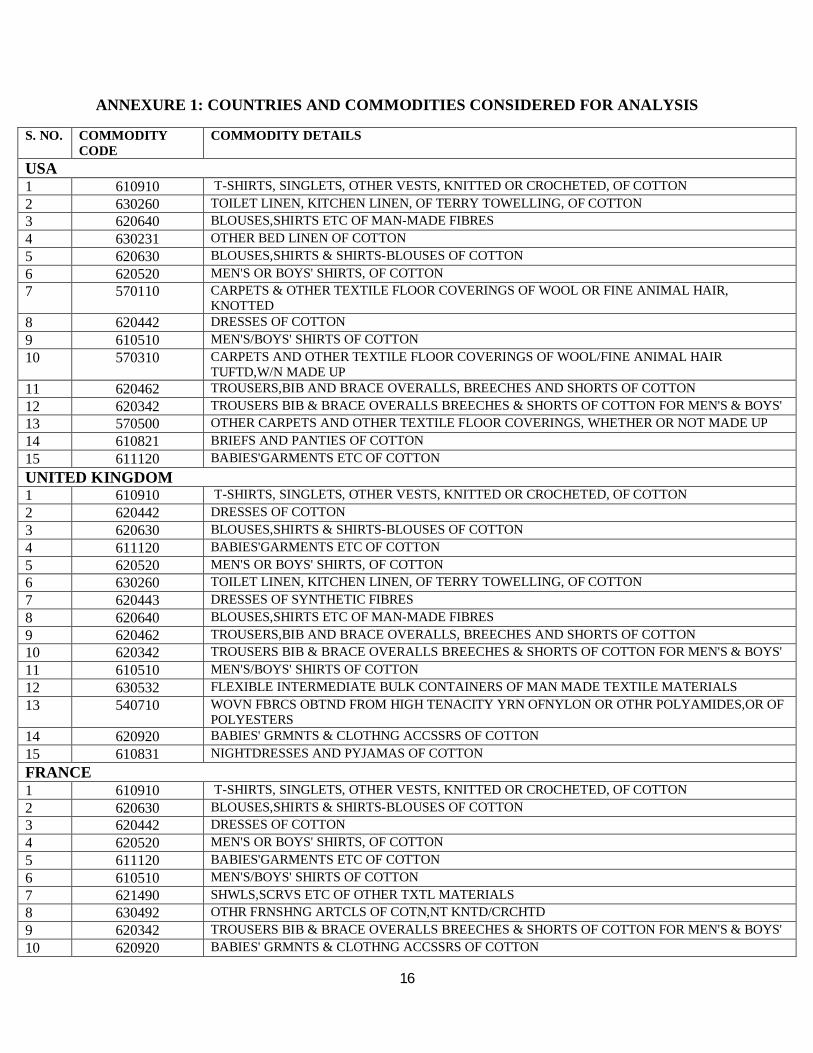
in current year. The top fifteen commodities for each country were selected based on the Mode
criterion i.e. the number of the times the commodity has appeared in the list of top 15
commodities for last 6 years i.e. from 2007 till 2012, from around 700 textile commodities traded
at 6-digit level of HS classification using Ministry of Commerce Export-import database. Along
with assessing the competitiveness of these commodities the forecasting of exports for these
commodities till the year 2015 is also attempted.
2. METHODOLOGY
The methodology used for generating the elasticities is the dynamic panel data approach. Within
broad category of dynamic panel data, Arellano Bond method has been used to estimate the price
and income elasticities for separate panels constructed for each export destination for top 15
textile products over the period of 12 years (2001-2012).
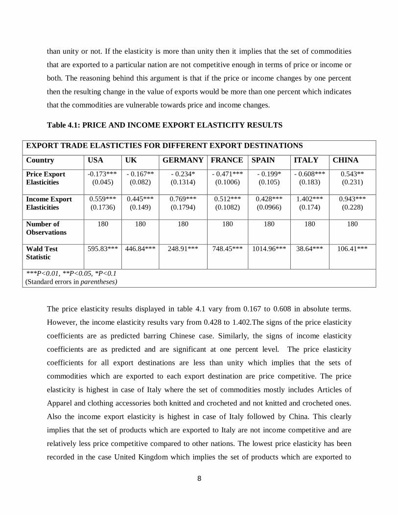
***P<0.01, **P<0.05, *P<0.1 (Standard errors in parentheses)
The price elasticity results displayed in table 4.1 vary from 0.167 to 0.608 in absolute terms.
However, the income elasticity results vary from 0.428 to 1.402.The signs of the price elasticity
coefficients are as predicted barring Chinese case. Similarly, the signs of income elasticity
coefficients are as predicted and are significant at one percent level. The price elasticity
coefficients for all export destinations are less than unity which implies that the sets of
commodities which are exported to each export destination are price competitive. The price
elasticity is highest in case of Italy where the set of commodities mostly includes Articles of
Apparel and clothing accessories both knitted and crocheted and not knitted and crocheted ones.
Also the income export elasticity is highest in case of Italy followed by China. This clearly
implies that the set of products which are exported to Italy are not income competitive and are
relatively less price competitive compared to other nations. The lowest price elasticity has been
recorded in the case United Kingdom which implies the set of products which are exported to
9
UK has strong demand and thus is not vulnerable to any price shocks. The set of products
exported to UK also includes mostly Articles of Apparel and clothing accessories both knitted
and crocheted. Thus, the exports to Italy and UK are more or less similar as they fall under the
category of articles knitted and crocheted. But the response to exports is starkly different when
the cases of UK and Italy are compared. The products exported to UK fare well in terms price
and income changes while the case of Italy has not been that strong. India has also performed
well in case of USA as the price elasticity is merely 0.173 which is next best after UK followed
by Spain where price elasticity for Indian exports is approximately 0.2 in absolute terms. The
products exported to china mostly include cotton yarn and man-made fibers. The price elasticity
for goods exported to china is positive which suggests that the raw products which are exported
to china are of Giffen good nature. However, the income elasticity is positive which implies that
the goods exported to china are not inferior.
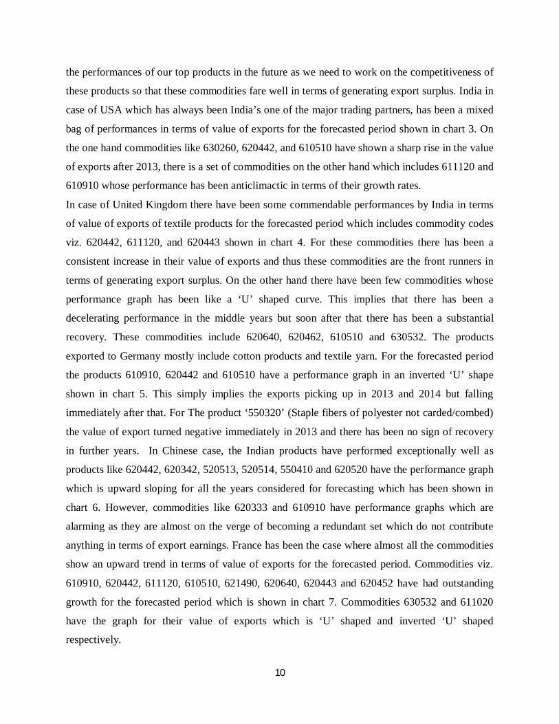
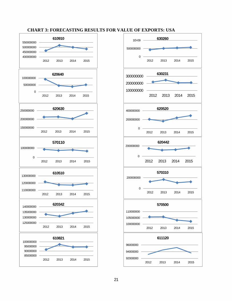
5. FORECASTING
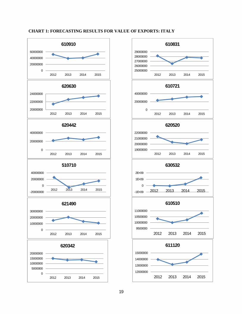
From chart 1 to chart 7 the forecasting results of different commodities exported to respective
export destinations are displayed. In chart 1 where forecasting results of Italy are presented, the
results are quite mixed in terms of performance. Commodities with HS Code2 610910, 610831,
620520, 510710, 610510, 630532 and 611120 show a decelerating growth rate in the year 2013.
Commodity code 510710, which is yarn of combed wool containing more than or equal to 85%
of wool, show a sharp decline in its value of exports in 2013 and value of exports in fact turn
negative which mean that we may end up importing this particular product in 2013. But after that
there are signs of recovery as the value of exports sharply rise at a significant growth rate. For
commodities 620630 and 610721 India show a precipitous increase in their value of exports to
Italy. For rest of the commodities the performance is not consistent as it wavers with time. In
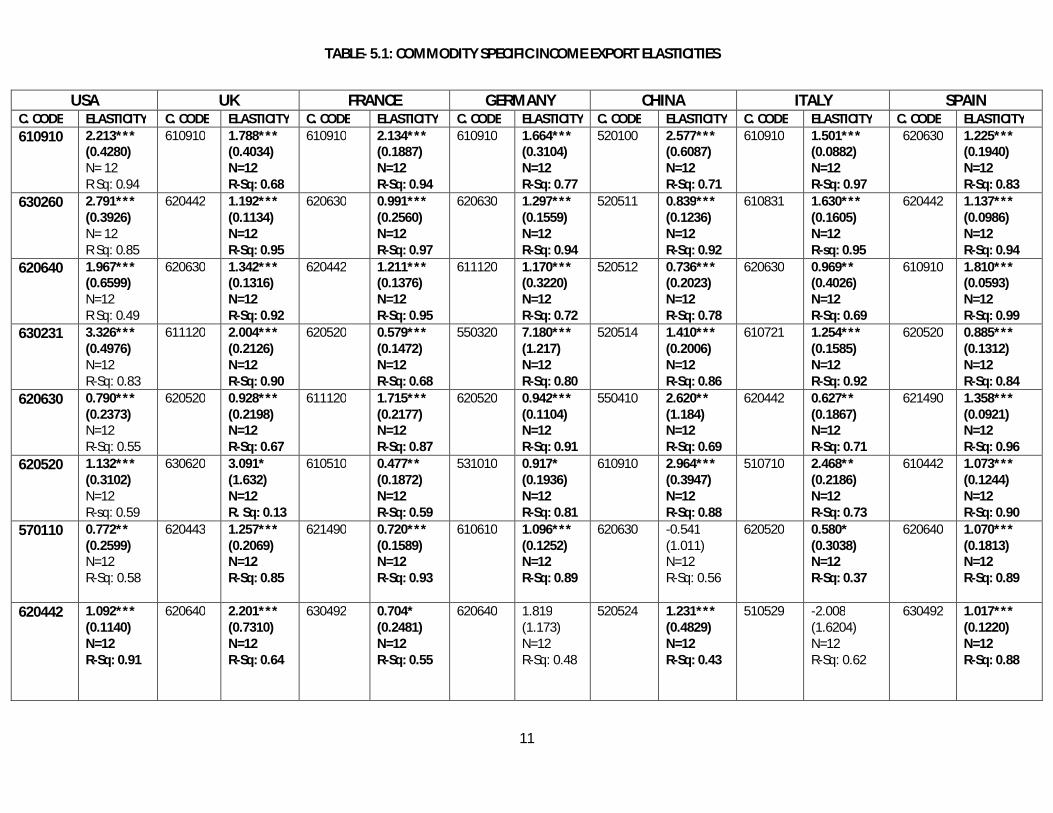
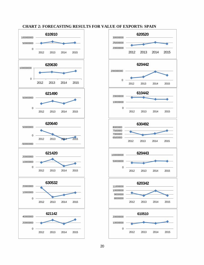
case of Spain the performance of the commodities is more or less stable barring few cases like
620640 which is Blouses, shirts etc. of man-made fibers where the value of exports again turns
out to be negative in 2014 whereas for commodity code 621420, 630532 the value of exports
almost touches the zero line in 2014 and 2013 respectively shown in chart 2. Commodities
620342,620443, 610442 and 620520 also show a dip in their performance in the year
2015.however, the fall is not as swift as the ones mentioned above. This raises concerns about
2 For detailed description of commodity codes refer to Annexure 1.
10
the performances of our top products in the future as we need to work on the competitiveness of
these products so that these commodities fare well in terms of generating export surplus. India in
case of USA which has always been India’s one of the major trading partners, has been a mixed
bag of performances in terms of value of exports for the forecasted period shown in chart 3. On
the one hand commodities like 630260, 620442, and 610510 have shown a sharp rise in the value
of exports after 2013, there is a set of commodities on the other hand which includes 611120 and
610910 whose performance has been anticlimactic in terms of their growth rates.
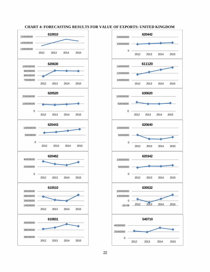
In case of United Kingdom there have been some commendable performances by India in terms
of value of exports of textile products for the forecasted period which includes commodity codes
viz. 620442, 611120, and 620443 shown in chart 4. For these commodities there has been a
consistent increase in their value of exports and thus these commodities are the front runners in
terms of generating export surplus. On the other hand there have been few commodities whose
performance graph has been like a ‘U’ shaped curve. This implies that there has been a
decelerating performance in the middle years but soon after that there has been a substantial
recovery. These commodities include 620640, 620462, 610510 and 630532. The products
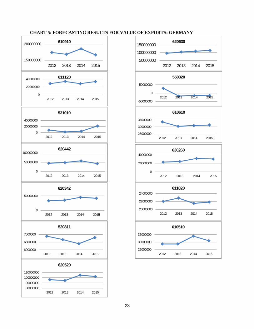
exported to Germany mostly include cotton products and textile yarn. For the forecasted period
the products 610910, 620442 and 610510 have a performance graph in an inverted ‘U’ shape
shown in chart 5. This simply implies the exports picking up in 2013 and 2014 but falling
immediately after that. For The product ‘550320’ (Staple fibers of polyester not carded/combed)
the value of export turned negative immediately in 2013 and there has been no sign of recovery
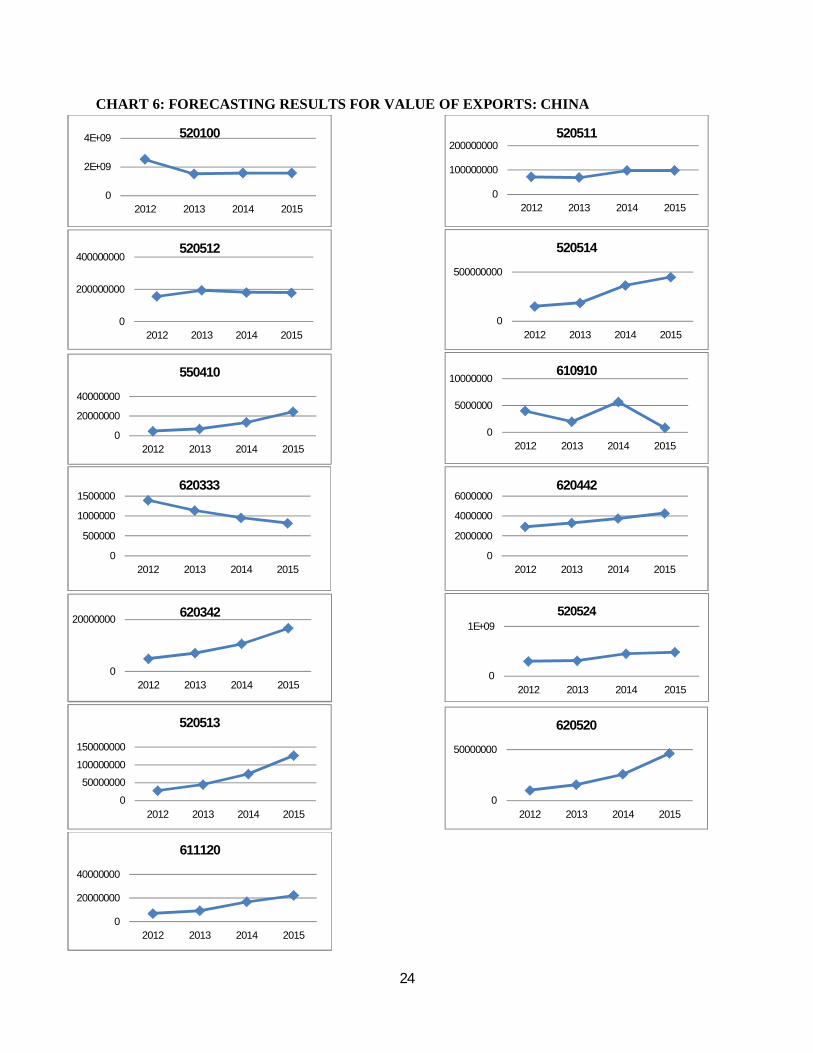
in further years. In Chinese case, the Indian products have performed exceptionally well as
products like 620442, 620342, 520513, 520514, 550410 and 620520 have the performance graph
which is upward sloping for all the years considered for forecasting which has been shown in
chart 6. However, commodities like 620333 and 610910 have performance graphs which are
alarming as they are almost on the verge of becoming a redundant set which do not contribute
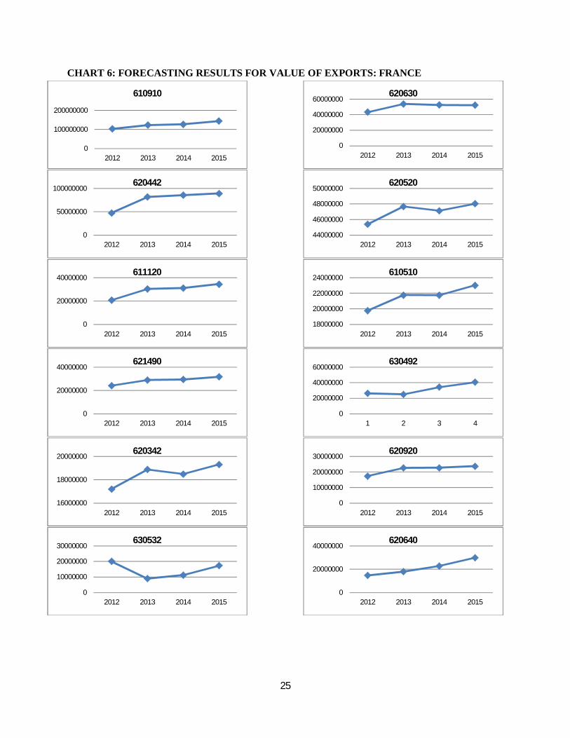
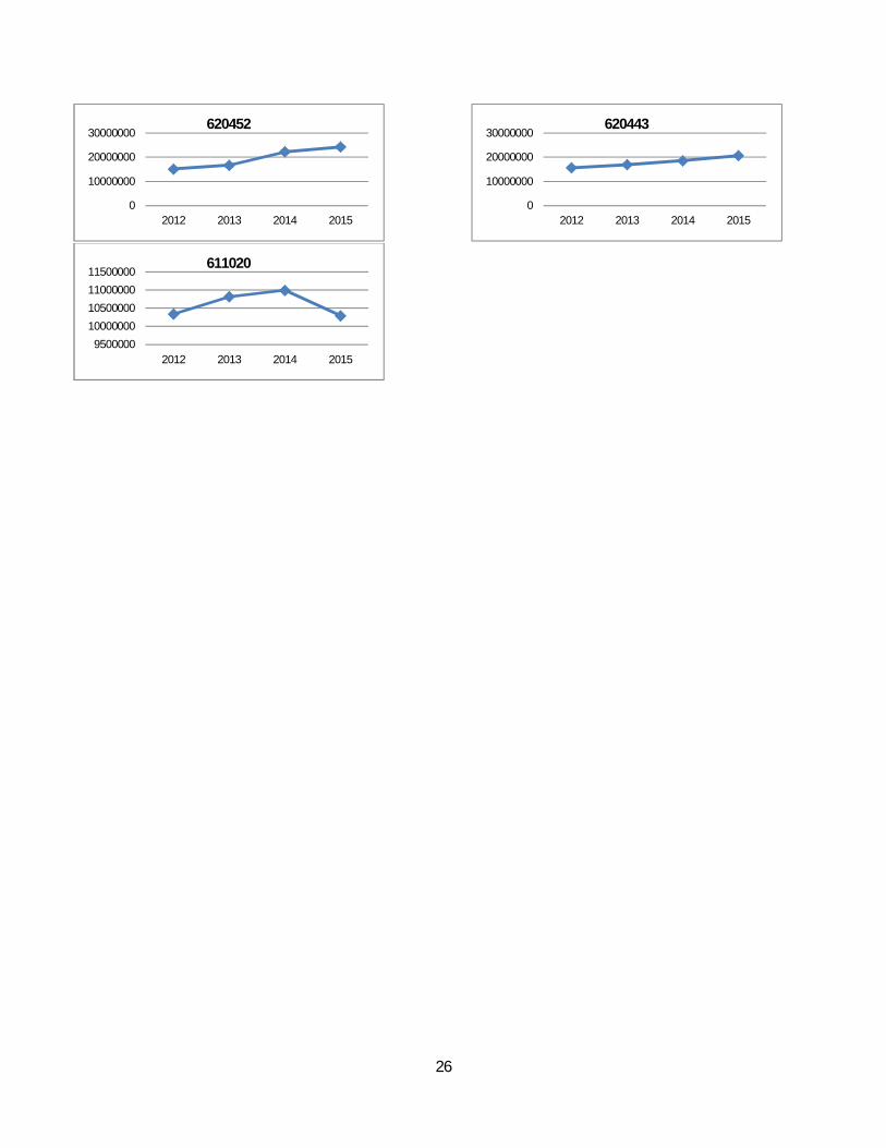
anything in terms of export earnings. France has been the case where almost all the commodities
show an upward trend in terms of value of exports for the forecasted period. Commodities viz.
610910, 620442, 611120, 610510, 621490, 620640, 620443 and 620452 have had outstanding
growth for the forecasted period which is shown in chart 7. Commodities 630532 and 611020
have the graph for their value of exports which is ‘U’ shaped and inverted ‘U’ shaped
respectively.
11
USA UK FRANCE GERMANY CHINA ITALY SPAIN C. CODE ELASTICITY C. CODE ELASTICITY C. CODE ELASTICITY C. CODE ELASTICITY C. CODE ELASTICITY C. CODE ELASTICITY C. CODE ELASTICITY 610910 2.213***
(0.4280) N= 12 R Sq: 0.94
610910 1.788*** (0.4034) N=12 R-Sq: 0.68
610910 2.134*** (0.1887) N=12 R-Sq: 0.94
610910 1.664*** (0.3104) N=12 R-Sq: 0.77
520100 2.577*** (0.6087) N=12 R-Sq: 0.71
610910 1.501*** (0.0882) N=12 R-Sq: 0.97
620630 1.225*** (0.1940) N=12 R-Sq: 0.83
630260 2.791*** (0.3926) N= 12 R Sq: 0.85
620442 1.192*** (0.1134) N=12 R-Sq: 0.95
620630 0.991*** (0.2560) N=12 R-Sq: 0.97
620630 1.297*** (0.1559) N=12 R-Sq: 0.94
520511 0.839*** (0.1236) N=12 R-Sq: 0.92
610831 1.630*** (0.1605) N=12 R-sq: 0.95
620442 1.137*** (0.0986) N=12 R-Sq: 0.94
620640 1.967*** (0.6599) N=12 R Sq: 0.49
620630 1.342*** (0.1316) N=12 R-Sq: 0.92
620442 1.211*** (0.1376) N=12 R-Sq: 0.95
611120 1.170*** (0.3220) N=12 R-Sq: 0.72
520512 0.736*** (0.2023) N=12 R-Sq: 0.78
620630 0.969** (0.4026) N=12 R-Sq: 0.69
610910 1.810*** (0.0593) N=12 R-Sq: 0.99
630231 3.326*** (0.4976) N=12 R-Sq: 0.83
611120 2.004*** (0.2126) N=12 R-Sq: 0.90
620520 0.579*** (0.1472) N=12 R-Sq: 0.68
550320 7.180*** (1.217) N=12 R-Sq: 0.80
520514 1.410*** (0.2006) N=12 R-Sq: 0.86
610721 1.254*** (0.1585) N=12 R-Sq: 0.92
620520 0.885*** (0.1312) N=12 R-Sq: 0.84
620630 0.790*** (0.2373) N=12 R-Sq: 0.55
620520 0.928*** (0.2198) N=12 R-Sq: 0.67
611120 1.715*** (0.2177) N=12 R-Sq: 0.87
620520 0.942*** (0.1104) N=12 R-Sq: 0.91
550410 2.620** (1.184) N=12 R-Sq: 0.69
620442 0.627** (0.1867) N=12 R-Sq: 0.71
621490 1.358*** (0.0921) N=12 R-Sq: 0.96
620520 1.132*** (0.3102) N=12 R-sq: 0.59
630620 3.091* (1.632) N=12 R. Sq: 0.13
610510 0.477** (0.1872) N=12 R-Sq: 0.59
531010 0.917* (0.1936) N=12 R-Sq: 0.81
610910 2.964*** (0.3947) N=12 R-Sq: 0.88
510710 2.468** (0.2186) N=12 R-Sq: 0.73
610442 1.073*** (0.1244) N=12 R-Sq: 0.90
570110 0.772** (0.2599) N=12 R-Sq: 0.58
620443 1.257*** (0.2069) N=12 R-Sq: 0.85
621490 0.720*** (0.1589) N=12 R-Sq: 0.93
610610 1.096*** (0.1252) N=12 R-Sq: 0.89
620630 -0.541 (1.011) N=12 R-Sq: 0.56
620520 0.580* (0.3038) N=12 R-Sq: 0.37
620640 1.070*** (0.1813) N=12 R-Sq: 0.89
620442 1.092*** (0.1140) N=12 R-Sq: 0.91
620640 2.201*** (0.7310) N=12 R-Sq: 0.64
630492 0.704* (0.2481) N=12 R-Sq: 0.55
620640 1.819 (1.173) N=12 R-Sq: 0.48
520524 1.231*** (0.4829) N=12 R-Sq: 0.43
510529 -2.008 (1.6204) N=12 R-Sq: 0.62
630492 1.017*** (0.1220) N=12 R-Sq: 0.88
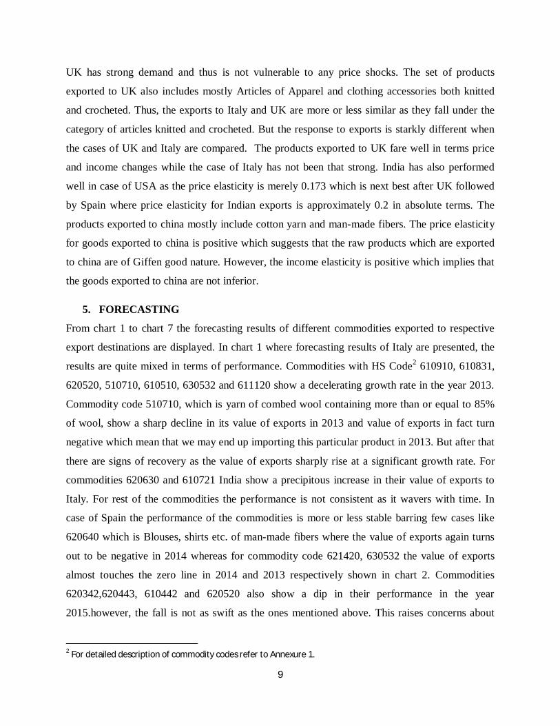
TABLE- 5.1: COMMODITY SPECIFIC INCOME EXPORT ELASTICITIES
12
610510 1.230*** (0.1941) N=12 R-sq: 0.82
620462 1.054*** (0.2953) N=12 R-Sq: 0.66
620342 1.243*** (0.2547) N=12 R-Sq: 0.87
630260 4.476*** (1.304) N=12 R-Sq: 0.65
620333 1.388** (0.6259) N=12 R-Sq: 0.47
520811 0.547 (0. 3762) N=12 R-Sq: 0.21
620342 0.830** (0.3245) N=12 R-Sq: 0.85
570310 1.878* (0.8320) N=12 R-sq: 0.44
620342 1.990*** (0.4928) N=12 R-Sq: 0.86
620920 1.143** (0.4047) N=12 R-Sq: 0.75
520811 0.8212*** (0.2202) N=12 R-Sq: 0.26
620442 2.905*** (0.4670) N=12 R-Sq: 0.87
620342 2.344*** (0.6269) N=12 R-Sq: 0.75
621420 2.150*** (0.7686) N=12 R-Sq: 0.55
620462 2.760 (2.436) N=12 R-Sq: 0.12
610510 0.892* (0.4154) N=12 R-Sq: 0.34
630532 3.135* (1.459) N=12 R-Sq: 0.91
620442 1.018*** (0.1184) N=12 R-Sq: 0.89
620342 1.909*** (0.6811) N=12 R-Sq: 0.82
630532 6.214** (1.947) N=12 R-Sq: 0.82
620443 0.956*** (0.1399) N=12 R-Sq: 0.85
620342 4.237** (1.393) N=12 R-Sq: 0.51
630532 8.026*** (1.5803) N=12 R-Sq: 0.77
620640 0.624** (0.2894) N=12 R-Sq: 0.41
570110 -1.107 (0.3224) N=12 R-Sq: 0.57
520513 1.842*** (0.5314) N=12 R-Sq: 0.60
611120 1.652*** (0.1243) N=12 R-Sq: 0.95
630532 5.507*** (0.8799) N=12 R-Sq: 0.83
570500 0.947** (0.3760) N=12 R-Sq: 0.64
540710 1.102* (0.5411) N=12 R-Sq: 0.81
620452 1.467*** (0.2571) N=12 R-Sq: 0.79
611020 0.793** (0.3359) N=12 R-Sq: 0.39
620520 3.288*** (1.245) N=12 R-Sq: 0.67
520548 0.826 (0.9886) N=12 R-Sq: 0.16
621142 1.520*** (0.5932) N=12 R-Sq: 0.59
610821 11.17** (4.738) N=12 R-Sq: 0.64
620920 0.499 (0.8060) N=12 R-Sq: 0.50
620443 0.506*** (0.1143) N=12 R-Sq: 0.68
620342 2.060*** (0.3951) N=12 R-Sq: 0.80
550330 1.471 (1.499) N=12 R-Sq: 0.57
621490 0.899*** (0.1292) N=12 R-Sq:0.93
540233 0.146 (1.033) N=12 0.27
611120 4.995*** (0.6247) N=12 R-Sq: 0.87
610831 0.922** (0.4984) N=12 R-Sq: 0.38
611020 0.735*** (0.2302) N=12 R-Sq: 0.56
610510 0.776*** (0.1915) N=12 R-Sq: 0.64
611120 1.800*** (0.3971) N=12 R-Sq: 0.74
610510 0.666*** (0.1767) N=12 R-Sq: 0.74
610510 0.734*** (0.1731) N=12 R-Sq: 0.87
***P<0.01, **P<0.05, *P<0.1 (Figures in the bold are the elasticities which have correct predicted sign and are significant at different levels)
13
The projections made for all the commodities for different export destinations have been more or
less heterogeneous. As shown in forecasts that no matter how well the commodities have
performed in the past in terms of export earnings but there is a risk that the performance of many
such commodities may dwindle down in the future. Thus, it is important to start thinking of some
strategy to make these commodities competitive and make sure the commodities which are
currently relatively competitive also remain the same in terms of their performance in the future.
6. CONCLUSION
Competitiveness has been the buzz word of today’s era and it is important in this current
globalized environment to be competitive given there is tremendous competition from rest of the
world in every sector. The aim of the whole exercise conducted above was to first try and assess
the trade competitiveness of top fifteen textile products exported to different countries and see
how competitive our top products have been in the past. This has been done by using the
Arellano Bond method for each panel of export destination. The average elasticities as
mentioned previously sort of corroborate the argument that Indian textile products are price and
income competitive barring the products which are exported to Italy which have recorded the
income elasticity of more than unity. However, the variation in the price elasticities across
nations has been more when compared to income elasticities. A product can be called as price
competitive if the unit cost of its production is much low in comparison to its counterparts and
thus has a low price without compromising on the quality of the same. After getting the average
elasticities the next step was to forecast the exports for the whole sample of commodities using
commodity specific income elasticities. The whole idea behind conducting this forecasting
exercise was to make sure in advance that the commodities which may lag behind in terms of
value of exports are focused upon and are made competitive with right policy interventions. It is
also important to understand that each export destination has its own peculiar characteristics and
if one policy gets implemented across all export destinations, which doesn’t take into
consideration the country specific needs, we are in a fix. There will be no way to understand why
one commodity is performing so well in one country and not so well in a different national
context. The bottom-line is that having a standard textile export policy for the whole sector will
not serve the purpose and we need to customize our policies with respect to each export
destination as we have clearly seen the response to almost similar articles exported to UK and
Italy is so different. Thus, it is important to draft country specific or export destination specific
14
textile policies rather than having a blanket policy for the whole sector. This analysis marks a
beginning of such kind of a work where each country has been separately considered. Also this
analysis is pertaining only to one sector which is also important as standard trade policies
devised for the entire trade sector will have no meaning. Once the results are obtained it is
important to understand the reason behind the lackluster performance of few commodities. The
commodities with a performance graph having downward sloping or ‘u’ shaped curves are the
ones which have to be checked for the reasons of their not so consistent performances. This
analysis can further be linked with the technical efficiency analysis to fathom out the reasons of
lack of competitiveness. There can be a clear case of lack of efficiency and productivity in
production of these commodities which has to be checked.
REFERENCES
Bobic, V. (2010). Income and Price elasticities of Croatian Trade – A panel data Approch. Croatian National Bank Working Paper, 25.
Hashim, D. (2005). Post MFA: Making the Textile and Garment Industry Competitive. Economic and Political Weekly, 40(2), 8-14.
Hauk, W. J. (2012). U.S. import and export elasticities: a panel data approach. Empirical Economics, 43, 73-96.
Hooper, P., Johnson, K., & Marquez, J. (2000, Aug). Trade elasticities for the G-7 countries. Princeton Studies in International economics, No.27.
Houthakker, H. S., & Magee, S. P. (1969, May). Income and Price elasticities in world trade. The Review of economics and statistics, 51(2), 111-125.
Imbs, J., & Méjean, I. (2010). Trade elasticities: A final report for the European commission. European commission economic Paper.
Kang, K. (2012). Is the “Houthakker-Magee” finding durable? Evidence from disaggregated trade flows between China and Korea. Annals of Economics and Finance, 13(2), 299-316.
Kee, H. L., Nicita, A., & Olarreaga, M. (2008, Nov). Import demand elasticities and trade distortions. The Review of Economics and Statistics, 90(4), 666-682.
15
Marquez, J., & McNeilly, C. (1988). Income and Price elasticities for exports of Developing Countries. The Review of economics and Statistics, 70(2), 306-314.
Mehta, R., & Mathur, P. (2004). India’s Exports by countries and commodies: On the estimation of a forecasting Model using Panel data. RIS- DP, 84.
Misra, S. (1993). India’s Textile Sector: A Policy Analysis. New Delhi: Sage Publications.
Roy, T. (1998, August). Economic Reforms and Textile Industry in India. Economic and Political Weekly, 33(32), 2173-2182.
Tokarick, S. (2010). A method for calculating export supply and Import demand elasticities. IMF working paper, WP/10/180.
16
ANNEXURE 1: COUNTRIES AND COMMODITIES CONSIDERED FOR ANALYSIS
S. NO. COMMODITY CODE
COMMODITY DETAILS
USA 1 610910 T-SHIRTS, SINGLETS, OTHER VESTS, KNITTED OR CROCHETED, OF COTTON 2 630260 TOILET LINEN, KITCHEN LINEN, OF TERRY TOWELLING, OF COTTON 3 620640 BLOUSES,SHIRTS ETC OF MAN-MADE FIBRES 4 630231 OTHER BED LINEN OF COTTON 5 620630 BLOUSES,SHIRTS & SHIRTS-BLOUSES OF COTTON 6 620520 MEN'S OR BOYS' SHIRTS, OF COTTON 7 570110 CARPETS & OTHER TEXTILE FLOOR COVERINGS OF WOOL OR FINE ANIMAL HAIR,
KNOTTED 8 620442 DRESSES OF COTTON 9 610510 MEN'S/BOYS' SHIRTS OF COTTON 10 570310 CARPETS AND OTHER TEXTILE FLOOR COVERINGS OF WOOL/FINE ANIMAL HAIR
TUFTD,W/N MADE UP 11 620462 TROUSERS,BIB AND BRACE OVERALLS, BREECHES AND SHORTS OF COTTON 12 620342 TROUSERS BIB & BRACE OVERALLS BREECHES & SHORTS OF COTTON FOR MEN'S & BOYS' 13 570500 OTHER CARPETS AND OTHER TEXTILE FLOOR COVERINGS, WHETHER OR NOT MADE UP 14 610821 BRIEFS AND PANTIES OF COTTON 15 611120 BABIES'GARMENTS ETC OF COTTON UNITED KINGDOM 1 610910 T-SHIRTS, SINGLETS, OTHER VESTS, KNITTED OR CROCHETED, OF COTTON 2 620442 DRESSES OF COTTON 3 620630 BLOUSES,SHIRTS & SHIRTS-BLOUSES OF COTTON 4 611120 BABIES'GARMENTS ETC OF COTTON 5 620520 MEN'S OR BOYS' SHIRTS, OF COTTON 6 630260 TOILET LINEN, KITCHEN LINEN, OF TERRY TOWELLING, OF COTTON 7 620443 DRESSES OF SYNTHETIC FIBRES 8 620640 BLOUSES,SHIRTS ETC OF MAN-MADE FIBRES 9 620462 TROUSERS,BIB AND BRACE OVERALLS, BREECHES AND SHORTS OF COTTON 10 620342 TROUSERS BIB & BRACE OVERALLS BREECHES & SHORTS OF COTTON FOR MEN'S & BOYS' 11 610510 MEN'S/BOYS' SHIRTS OF COTTON 12 630532 FLEXIBLE INTERMEDIATE BULK CONTAINERS OF MAN MADE TEXTILE MATERIALS 13 540710 WOVN FBRCS OBTND FROM HIGH TENACITY YRN OFNYLON OR OTHR POLYAMIDES,OR OF
POLYESTERS 14 620920 BABIES' GRMNTS & CLOTHNG ACCSSRS OF COTTON 15 610831 NIGHTDRESSES AND PYJAMAS OF COTTON FRANCE 1 610910 T-SHIRTS, SINGLETS, OTHER VESTS, KNITTED OR CROCHETED, OF COTTON 2 620630 BLOUSES,SHIRTS & SHIRTS-BLOUSES OF COTTON 3 620442 DRESSES OF COTTON 4 620520 MEN'S OR BOYS' SHIRTS, OF COTTON 5 611120 BABIES'GARMENTS ETC OF COTTON 6 610510 MEN'S/BOYS' SHIRTS OF COTTON 7 621490 SHWLS,SCRVS ETC OF OTHER TXTL MATERIALS 8 630492 OTHR FRNSHNG ARTCLS OF COTN,NT KNTD/CRCHTD 9 620342 TROUSERS BIB & BRACE OVERALLS BREECHES & SHORTS OF COTTON FOR MEN'S & BOYS' 10 620920 BABIES' GRMNTS & CLOTHNG ACCSSRS OF COTTON
17
11 630532 FLEXIBLE INTERMEDIATE BULK CONTAINERS OF MAN MADE TEXTILE MATERIALS 12 620640 BLOUSES,SHIRTS ETC OF MAN-MADE FIBRES 13 620452 SKIRTS AND DIVIDED SKIRTS OF COTTON 14 620443 DRESSES OF SYNTHETIC FIBRES 15 611020 JERSEYS ETC OF COTTON GERMANY 1 610910 T-SHIRTS, SINGLETS, OTHER VESTS, KNITTED OR CROCHETED, OF COTTON 2 620630 BLOUSES,SHIRTS & SHIRTS-BLOUSES OF COTTON 3 611120 BABIES'GARMENTS ETC OF COTTON 4 550320 STAPLE FIBRES OF POLYESTER NT CRD/CMBD 5 620520 MEN'S OR BOYS' SHIRTS, OF COTTON 6 531010 UNBLECHD WOVEN FABRICS OF JUTE/OTHER TEXTILE BAST FIBRES 7 610610 BLOUSE ETC OF COTTON 8 620640 BLOUSES,SHIRTS ETC OF MAN-MADE FIBRES 9 630260 TOILET LINEN, KITCHEN LINEN, OF TERRY TOWELLING, OF COTTON 10 520811 COTN FABRCS CONTNG>=85% BY WT OF COTN, UNBLEACHED PLAIN WEAVE WEIGING
<=100 G/M2 11 620442 DRESSES OF COTTON 12 570110 CARPETS & OTHER TEXTILE FLOOR COVERINGS OF WOOL OR FINE ANIMAL HAIR,
KNOTTED 13 611020 JERSEYS ETC OF COTTON 14 620342 TROUSERS BIB & BRACE OVERALLS BREECHES & SHORTS OF COTTON FOR MEN'S & BOYS' 15 610510 MEN'S/BOYS' SHIRTS OF COTTON CHINA 1 520100 COTTON, NOT CARDED OR COMBED 2 520511 SNGL YRN OF UNCMBD FBRS MEASURNG 714.29 DCTX/MORE(NT EXCDNG 14 MTRC NO) 3 520512 SNGL YRN OF UNCMBD FBRS MEASURING= 232.56 DCTX(> 14 BUT <=43 MTRC NO) 4 520514 SNGL YRN OF UNCMBD FBRS MEASURNG=125 DCTX(>50 BUT <=80 MTRC NO) 5 550410 VISCOSE RAYON STAPLE FIBRES NT CRD/COMBD 6 610910 T-SHIRTS, SINGLETS, OTHER VESTS, KNITTED OR CROCHETED, OF COTTON 7 620630 BLOUSES,SHIRTS & SHIRTS-BLOUSES OF COTTON 8 520524 SNGL YRN OF CMBD FBRS MEASURNG=125 DCTX(>52 BUT <=80 MTRC NO) 9 620333 JACKTS & BLAZERS OF SYNTHETIC FIBRES 10 620442 DRESSES OF COTTON 11 620342 TROUSERS BIB & BRACE OVERALLS BREECHES & SHORTS OF COTTON FOR MEN'S & BOYS' 12 520513 SNGL YRN OF UNCMBD FBRS MEASURNG=192.31 DCTX(>43 BUT <=52 MTRC NO) 13 620520 MEN'S OR BOYS' SHIRTS, OF COTTON 14 550330 STAPLE FIBRS OF ACRLC/MODACRLC NT CRD/CMBD 15 611120 BABIES'GARMENTS ETC OF COTTON ITALY 1 610910 T-SHIRTS, SINGLETS, OTHER VESTS, KNITTED OR CROCHETED, OF COTTON 2 610831 NIGHTDRESSES AND PYJAMAS OF COTTON 3 620630 BLOUSES,SHIRTS & SHIRTS-BLOUSES OF COTTON 4 610721 NIGHTSHIRTS & PYJAMAS OF COTTON 5 620442 DRESSES OF COTTON 6 510710 YARN OF COMBED WOOL CONTNG>=85% WOOL BY WTNOT PUT UP FOR RETAIL SALE 7 620520 MEN'S OR BOYS' SHIRTS, OF COTTON 8 510529 WOOL TOPS AND OTHER COMBED WOOL 9 520811 COTN FABRCS CONTNG>=85% BY WT OF COTN, UNBLEACHED PLAIN WEAVE WEIGING
18
<=100 G/M2 10 620342 TROUSERS BIB & BRACE OVERALLS BREECHES & SHORTS OF COTTON FOR MEN'S & BOYS' 11 630532 FLEXIBLE INTERMEDIATE BULK CONTAINERS OF MAN MADE TEXTILE MATERIALS 12 611120 BABIES'GARMENTS ETC OF COTTON 13 520548 MLTPL (FOLDD)/CABLD YRN OF COMBD FBRS MSRNG PER SNGL YRN 120 MTRC NO. 14 621490 SHWLS,SCRVS ETC OF OTHER TXTL MATERIALS 15 610510 MEN'S/BOYS' SHIRTS OF COTTON SPAIN 1 620630 BLOUSES,SHIRTS & SHIRTS-BLOUSES OF COTTON 2 620442 DRESSES OF COTTON 3 610910 T-SHIRTS, SINGLETS, OTHER VESTS, KNITTED OR CROCHETED, OF COTTON 4 620520 MEN'S OR BOYS' SHIRTS, OF COTTON 5 621490 SHWLS,SCRVS ETC OF OTHER TXTL MATERIALS 6 610442 DRESSES OF COTTON 7 620640 BLOUSES,SHIRTS ETC OF MAN-MADE FIBRES 8 630492 OTHR FRNSHNG ARTCLS OF COTN,NT KNTD/CRCHTD 9 620342 TROUSERS BIB & BRACE OVERALLS BREECHES & SHORTS OF COTTON FOR MEN'S & BOYS' 10 621420 SHWLS,SCARVES ETC OF WOOL/FINE ANML HAIR 11 620443 DRESSES OF SYNTHETIC FIBRES 12 630532 FLEXIBLE INTERMEDIATE BULK CONTAINERS OF MAN MADE TEXTILE MATERIALS 13 621142 OTHR GRMNTS OF COTTON FR WOMEN'S OR GIRLS' 14 540233 TEXTURED YARN OF POLYESTERS 15 610510 MEN'S/BOYS' SHIRTS OF COTTON
19
CHART 1: FORECASTING RESULTS FOR VALUE OF EXPORTS: ITALY
0
20000000
40000000
60000000
2012 2013 2014 2015
610910
2500000026000000270000002800000029000000
2012 2013 2014 2015
610831
20000000
22000000
24000000
2012 2013 2014 2015
620630
0
20000000
40000000
2012 2013 2014 2015
610721
0
20000000
40000000
2012 2013 2014 2015
620442
19000000
20000000
21000000
22000000
2012 2013 2014 2015
620520
-20000000
0
20000000
40000000
2012 2013 2014 2015
510710
-1E+09
0
1E+09
2E+09
2012 2013 2014 2015
630532
0
10000000
20000000
30000000
2012 2013 2014 2015
621490
9500000
10000000
10500000
11000000
2012 2013 2014 2015
610510
0
5000000
1000000015000000
20000000
2012 2013 2014 2015
620342
12000000
13000000
14000000
15000000
2012 2013 2014 2015
611120
20
CHART 2: FORECASTING RESULTS FOR VALUE OF EXPORTS: SPAIN
0
50000000
100000000
2012 2013 2014 2015
610910
20000000
25000000
30000000
2012 2013 2014 2015
620520
0
100000000
2012 2013 2014 2015
620630
0
200000000
2012 2013 2014 2015
620442
0
50000000
2012 2013 2014 2015
621490
0
10000000
20000000
2012 2013 2014 2015
610442
-50000000
0
50000000
2012 2013 2014 2015
620640
6500000700000075000008000000
2012 2013 2014 2015
630492
0
10000000
20000000
2012 2013 2014 2015
621420
0
50000000
100000000
2012 2013 2014 2015
620443
0
10000000
20000000
2012 2013 2014 2015
630532
80000009000000
1000000011000000
2012 2013 2014 2015
620342
0
20000000
40000000
2012 2013 2014 2015
621142
0
10000000
20000000
2012 2013 2014 2015
610510
21
CHART 3: FORECASTING RESULTS FOR VALUE OF EXPORTS: USA
400000000
450000000500000000
550000000
2012 2013 2014 2015
610910
0
500000000
1E+09
2012 2013 2014 2015
630260
0
50000000
100000000
2012 2013 2014 2015
620640
100000000
200000000
300000000
2012 2013 2014 2015
630231
150000000
200000000
250000000
2012 2013 2014 2015
620630
0
200000000
400000000
2012 2013 2014 2015
620520
0
100000000
2012 2013 2014 2015
570110
0
200000000
2012 2013 2014 2015
620442
110000000
120000000
130000000
2012 2013 2014 2015
610510
0
200000000
2012 2013 2014 2015
570310
125000000
130000000
135000000
140000000
2012 2013 2014 2015
620342
100000000
105000000
110000000
2012 2013 2014 2015
570500
850000009000000095000000
100000000
2012 2013 2014 2015
610821
92000000
94000000
96000000
2012 2013 2014 2015
611120
22
CHART 4: FORECASTING RESULTS FOR VALUE OF EXPORTS: UNITED KINGDOM
130000000
140000000
150000000
2012 2013 2014 2015
610910
0
100000000
200000000
2012 2013 2014 2015
620442
70000000
80000000
90000000
100000000
2012 2013 2014 2015
620630
100000000
120000000
140000000
2012 2013 2014 2015
611120
0
100000000
200000000
2012 2013 2014 2015
620520
0
50000000
100000000
2012 2013 2014 2015
630620
0
50000000
100000000
2012 2013 2014 2015
620443
0
50000000
100000000
2012 2013 2014 2015
620640
0
20000000
40000000
2012 2013 2014 2015
620462
0
50000000
100000000
2012 2013 2014 2015
620342
24000000
26000000
28000000
30000000
2012 2013 2014 2015
610510
-1E+08
0
100000000
200000000
2012 2013 2014 2015
630532
36000000
38000000
40000000
2012 2013 2014 2015
610831
0
20000000
40000000
2012 2013 2014 2015
540710
23
CHART 5: FORECASTING RESULTS FOR VALUE OF EXPORTS: GERMANY
150000000
200000000
2012 2013 2014 2015
610910
50000000
100000000
150000000
2012 2013 2014 2015
620630
0
20000000
40000000
2012 2013 2014 2015
611120
-50000000
0
50000000
2012 2013 2014 2015
550320
0
20000000
40000000
2012 2013 2014 2015
531010
25000000
30000000
35000000
2012 2013 2014 2015
610610
0
50000000
100000000
2012 2013 2014 2015
620442
0
20000000
40000000
2012 2013 2014 2015
630260
0
50000000
2012 2013 2014 2015
620342
20000000
22000000
24000000
2012 2013 2014 2015
611020
6000000
6500000
7000000
2012 2013 2014 2015
520811
25000000
30000000
35000000
2012 2013 2014 2015
610510
8000000090000000
100000000110000000
2012 2013 2014 2015
620520
24
CHART 6: FORECASTING RESULTS FOR VALUE OF EXPORTS: CHINA
0
2E+09
4E+09
2012 2013 2014 2015
520100
0
100000000
200000000
2012 2013 2014 2015
520511
0
200000000
400000000
2012 2013 2014 2015
520512
0
500000000
2012 2013 2014 2015
520514
0
20000000
40000000
2012 2013 2014 2015
550410
0
5000000
10000000
2012 2013 2014 2015
610910
0
500000
1000000
1500000
2012 2013 2014 2015
620333
0
2000000
4000000
6000000
2012 2013 2014 2015
620442
0
20000000
2012 2013 2014 2015
620342
0
1E+09
2012 2013 2014 2015
520524
0
50000000
100000000
150000000
2012 2013 2014 2015
520513
0
50000000
2012 2013 2014 2015
620520
0
20000000
40000000
2012 2013 2014 2015
611120
25
CHART 6: FORECASTING RESULTS FOR VALUE OF EXPORTS: FRANCE