This article was downloaded by: [University of Sydney] On: 26 April 2013, At: 02:33 Publisher: Taylor & Francis Informa Ltd Registered in England and Wales Registered Number: 1072954 Registered office: Mortimer House, 37-41 Mortimer Street, London W1T 3JH, UK Advances in Physics Publication details, including instructions for authors and subscription information: http://www.tandfonline.com/loi/tadp20 Expressing the decoupled equations of motion for the Green's function as a partial sum of Feynman diagrams R.D. Mattuck a & Alba Theumann b a Physics Laboratory I, H. C. Ørsted Institute, University of Copenhagen, 2100, Copenhagen Ø, Denmark b Institute for Theoretical Physics, Technical University of Norway, Trondheim, Norway Version of record first published: 28 Jul 2006. To cite this article: R.D. Mattuck & Alba Theumann (1971): Expressing the decoupled equations of motion for the Green's function as a partial sum of Feynman diagrams, Advances in Physics, 20:88, 721-745 To link to this article: http://dx.doi.org/10.1080/00018737100101331 PLEASE SCROLL DOWN FOR ARTICLE Full terms and conditions of use: http://www.tandfonline.com/page/terms-and-conditions This article may be used for research, teaching, and private study purposes. Any substantial or systematic reproduction, redistribution, reselling, loan, sub-licensing, systematic supply, or distribution in any form to anyone is expressly forbidden. The publisher does not give any warranty express or implied or make any representation that the contents will be complete or accurate or up to date. The accuracy of any instructions, formulae, and drug doses should be independently verified with primary sources. The publisher shall not be liable for any loss, actions, claims, proceedings, demand, or costs or damages whatsoever or howsoever caused arising directly or indirectly in connection with or arising out of the use of this material.
Transcript
This article was downloaded by: [University of Sydney]On: 26 April 2013, At: 02:33Publisher: Taylor & FrancisInforma Ltd Registered in England and Wales Registered Number: 1072954 Registeredoffice: Mortimer House, 37-41 Mortimer Street, London W1T 3JH, UK
Advances in PhysicsPublication details, including instructions for authors andsubscription information:http://www.tandfonline.com/loi/tadp20
Expressing the decoupled equations ofmotion for the Green's function as apartial sum of Feynman diagramsR.D. Mattuck a & Alba Theumann ba Physics Laboratory I, H. C. Ørsted Institute, University ofCopenhagen, 2100, Copenhagen Ø, Denmarkb Institute for Theoretical Physics, Technical University of Norway,Trondheim, NorwayVersion of record first published: 28 Jul 2006.
To cite this article: R.D. Mattuck & Alba Theumann (1971): Expressing the decoupled equations ofmotion for the Green's function as a partial sum of Feynman diagrams, Advances in Physics, 20:88,721-745
To link to this article: http://dx.doi.org/10.1080/00018737100101331
PLEASE SCROLL DOWN FOR ARTICLE
Full terms and conditions of use: http://www.tandfonline.com/page/terms-and-conditions
This article may be used for research, teaching, and private study purposes. Anysubstantial or systematic reproduction, redistribution, reselling, loan, sub-licensing,systematic supply, or distribution in any form to anyone is expressly forbidden.
The publisher does not give any warranty express or implied or make any representationthat the contents will be complete or accurate or up to date. The accuracy of anyinstructions, formulae, and drug doses should be independently verified with primarysources. The publisher shall not be liable for any loss, actions, claims, proceedings,demand, or costs or damages whatsoever or howsoever caused arising directly orindirectly in connection with or arising out of the use of this material.
Expressing the Decoupled Equations of Motion for the Green's Function as a Partial Sum of Fey nma n Diagrams
By R. D. N[ATTUCK Physics Laboratory I, H. C. Orsted Institute, University of Copenhagen,
2100 Copenhagen 0, Denmark
and ALBA THEUMA~N Institute for Theoretical Physics, Technical University of Norway,
Trondheim, Norway
A B S T R A C T
I t is s h o w n t h a t a n y g iven decoupl ing of t he equa t ions of m o t i o n for t h e p ropaga to r s o f a n in t e rac t ing F e r m i s y s t e m is equ iva l en t to a pa r t i cu la r pa r t i a l s u m of F e y n m a n d iag rams . This resu l t is e s tab l i shed for m a n y - t i m e p ropaga to r s in a s t r a i g h t f o r w a r d w a y by i t e ra t ing in t he d i a g r a m m a t i c f o rm of t h e equa t ions o f mot ion . T h e i te ra t ion m e t h o d does n o t work for two- t ime p ropaga to rs , b u t we are able to p re sen t an a l t e rna t ive a r g u m e n t wh ich m a k e s it p lausible t h a t t h e resu l t ho lds t rue in th i s case as well. The decoupl ings l ead ing to t h e H a r t r e e - F o e k , ladder , a n d r ing d i a g r a m (RPA) pa r t i a l s u m s are d iscussed in detai l . I t is con jec tu red t h a t t he reverse cor respondence is n o t t rue , i.e. to a n y g iven pa r t i a l s u m there does n o t necessar i ly cor respond a decoupl ing.
C O N T E N T S PAGE
§ 1. INTRODUCTION. 722
§ 2. REVIEW OF THE PARTIAL SUM METHOD. 723
§ 3. REVIEW OF THE DECOUPLING METHOD FOI¢ MANY-TIME PRO- FAGATOI%S. 727
§ 4. DIAGRAMIVfATIC P~EPRESENTATION OF THE EQUATIONS OF MOTION.
§ 5. DECOUPLED EQUATION OF MOTION EXPRESSED AS A PARTIAL SUIte. 5.1. Hartree~Fock A p p r o x i m a t i o n . 5.2. L a d d e r A p p r o x i m a t i o n . 5.3. A n t i s y m m e t r i z e d L a d d e r Approx ima t ion . 5.4. R a n d o m - p h a s e A p p r o x i m a t i o n (Ring Diagram) . 5.5. Decoupled E q u a t i o n s of Mot ion wh ich do no t lead to a D y s o n
E q u a t i o n . 5.6. Higher -o rde r Decoupl ing .
§ 6. DECOUPLING IN CONDENSED SYSTElg$.
§ 7. DOES EVEI%Y PARTIAL SU~¢i HAVE AN EQUIVALENT DECOUPLIIVG ?
§ 8. TWO-TIME IOROPAGATORS.
§ 9. CONCLUSION.
ACKNOWLEDGlV[E:NT.
732
732 733 734 735 735
738 739
739
740
741
744
744
REFERENCES. 745
Dow
nloa
ded
by [
Uni
vers
ity o
f Sy
dney
] at
02:
33 2
6 A
pril
2013
722 R. D. Mattuck and A. Theumann on
§ ]. ~NTRODUCTION GREEN'S functions, or ' propagators ', are among the most powerful tools known for calculating the physical properties of strongly interacting many-body systems. They yield in a simple, direct manner the energy of the ground state, the dispersion law of the elementary excitations, the electrical resistance, the magnetic susceptibility, etc. Therefore a considerable amount of effort in recent years has gone into computing the propagators for various physical systems.
There are two general methods available for finding propagators. The first involves solving an infinite hierarchy of differential equations connecting propagators of successively higher order (Martin and Schwinger 1959, Kadanoff and Baym 1962, Zubarev 1960, Bonch-Bruevieh and Tyablikov 1962). The other requires summing an infinite series of terms or Feynman diagrams in the perturbation expansion of the pro- pagator (Mattuck ]967, Schultz ]964, Abrikosov et al. 1963, Nozi~res 1964). Klein (1962), and later Kobe (1966), have shown that the perturba- tion expansion can be generated directly from the equations of motion, thus establishing the equivalence of the two methods when they are carried out exactly. But when actually solving a problem, we are forced to use approximation techniques. In the equation-of-motion case, the usual technique is to decouple the hierarchy of equations by expressing some higher-order propagator in terms of lower-order ones. In the perturbation expansion case, one carries out a sun] over just a certain subclass of Feynman diagrams in the expansion, i.e. a partial sum.
The question to be considered here is the following: we know that the equation-of-motion method for finding the propagator is formally equivalent to the Feynman diagram perturbation method. But is the decoupling approximation used in the equation-of-motion method equivalent to the partial sum approximation used in the perturbation method?
Doman (1967) and Gluck (1967) have examined this question in a couple of special cases. We carry the investigation further, and by iterating in the diagrammatic form of the decoupled equations of motion show that to each given decoupling approximation for the propagator, there corresponds an equivalent partial sum. In this way we build a bridge between physicists using equations of motion and those using Feynman diagrams. That is, given any equation-of-motion calculation, one can immediately see what it means in terms of summing over diagrams.
However, it seems that traffic on the bridge moves only in one direction, i.e. decoupling-+partial sum. We have not been able to show that to each given partial sum there corresponds an equivalent dccoupling, and indeed we suspect, for reasons to be discussed (see §7) that this reverse correspondence is not true.
We have only been able to establish our results rigorously for the case of many-time propagators. Two-time propagators are more stubborn because the two-time equations of motion cannot be expressed in terms of
Dow
nloa
ded
by [
Uni
vers
ity o
f Sy
dney
] at
02:
33 2
6 A
pril
2013
Decoupled Green's Functions and Diagrams 723
Feynman diagrams. However, we are able to present a rough argument (see § 8) which we feel makes it plausible t ha t our conclusions m a y also be true in the two-t ime case.
In the next two sections we review the part ial sum and decoupled equation-of-motion methods for obtaining the many- t ime Green's function. In § 4 it is shown how to express the equation of motion diagrammatical ly, and in § 5 we exhibit the deconplings leading to the Har t ree -Fock ladder, and ring (gPA) part ial sums. Deeoupling in condensed systems is t rea ted in § 6. The two-t ime ease is discussed in § 8. I t should be mentioned tha t al though we work at zero temperature for simplicity, our a rgument may be carried over immedia te ly to the finite temperature case by just subst i tut ing finite temperature propagators for the zero temperature ones.
§ 2. REVIEW OF THE ~PAgTIAL SUM METHOD
Imagine tha t we have a system of identical fermions interacting by means of a two-body force, and assume tha t there is no external potential . The Hamil tonian is then
H = fdr¢*(r)(- 2~)¢(r)+ ½f fdr dr' Ct(r)¢t(r')v(r- r')¢(r')¢(r), (1)
where ]~= l, r e=par t ic le mass, v ( r - r ' ) is the interaction potential , and ~b+(r), ¢(r) are operators which respectively create and destroy a particle at point r. The ¢ obey the ant icomuta t ion relations
Spin variables have been suppressed for brevity. The single particle propagator for this system is defined by
G(1 ;1 ' )= - i(T{~b(1)~bt(l')}), . . . . . (3)
where 1= (r i, tl), 1'= (rl', tl' ), ( . . . . . } means average over the exact ground state of the interacting system and T is the t ime-ordering operator. (In the finite temperature generalization of eqn. (3), ( . . . . ) s tands for the average over a grand canonical ensemble at a finite temperature.) In the case of a 'normal ' or 'non.-condensed' system, this propagator m a y be expanded in a per turbat ion series with the aid of F e y n m a n diagrams, as shown in fig. 1. These diagrams may be t ranslated into functions by means of the rules (see Mat tuck (1967)) :
1. The double line with the arrow is the exact or 'clothed' single particle propagator iG(i ;j).
2. Single lines with arrows are bare propagators, iGo(i ;j). 3. Wiggly lines are interactions, -iv(i ;j). 4. In tegrate over all intermediate space-t ime variables, and sum ever
intermediate spins. 5. Associate a factor of - 1 wi th each fermion loop. Each diagram in fig. 1 consists of a main line running from 1' to 1,
together with zero, one, or more 'proper self-energy parts ' inserted into
Dow
nloa
ded
by [
Uni
vers
ity o
f Sy
dney
] at
02:
33 2
6 A
pril
2013
724
1
1~. D. Mat tuck and A. Theumann on
+;+ 2
Fig. 1
3 4 5 6
4-. . .
+ ~ ) +...+
7 8 9 10
11 12
. . . . . . . . . .
13 14 Perturbation expansion of the single particle propagator.
(a) I I I
1' 1'
Fig. 2
1 1 1
1' 1'
1 2 3 4 5 6 7
(a), (b) Dyson's equation, (c) series for the proper self-energy, ~, (d) self-consistent form of ~.
Dow
nloa
ded
by [
Uni
vers
ity o
f Sy
dney
] at
02:
33 2
6 A
pril
2013
Decoupled Green's Functions and Diagrams 725
this main line. The series may be evaluated approximately by summing to infinite order over diagrams having certain types of proper self-energy par~s ('partial sum'). For example, a sum over all diagrams containing repeated proper self-energy parts of the 'bubble' and 'open oyster' type, e.g. diagrams 1,2,3,5,7,8,.... in fig. i yield the Hart ree-Fock approximation. Summing over diagrams with repeated parts of the 'ring' type, such as 1,3,4,10,11,.... gives the random phase approximation (RPA), while the sum over 1,2,3,4,5,6,7,8,12,13,14,.... is the ladder approximation. In general, sums over all repeated proper self-energy parts of a certain type or types yields an equation of the form shown in fig. 2 (a), (b) and known as Dyson's equation. In this figure, ~ , which is the sum over all the types of proper self-energy parts which have been included in the partial sum, is called the 'proper self-energy'. For example, in Hartree-]?ock approxima- tion, ~ is given by fig. 2 (c) : 1 + 2. In RPA, ~ = 2 + 3 + 6 . . . .
When the propagators appearing in the proper self-energy parts are clothed, ~ has the form shown in fig. 2 (d) and we have 'self-consistent perturbation theory'.
I t is important to observe that there are atso partial sums which do not include any repeated proper self-energy parts, and therefore do not yield a result having the Dyson form fig. 2 (a), (b). An example of this is the sum over all diagrams containing just a single proper self-energy part of the ladder type, i.e. the sum of 1,2,4,12, 14,. . . in fig. 1. We can also have partial sums in which some proper self-energy parts are repeated and some are not ; these evidently do not produce the result of fig. 2 (a), (b) either.
Equation (3) may be generalized to the many-time n-particle propagator, Gn, defined by
Note that G n changes sign when we exchange any two variables :
G n ( 1 . . . i . . . j . . . n ; l ' . . . n ' ) = ( - 1 ) G n ( 1 . . . j . . . i . . . n ; l ' . . . n ' ) , t G~(1 . . n ; l ' . . . i ' . . . j ' .n ' )=(-1)G~(1. . .n; l ' . j ' . . . i ' . . . n ) . , (6)
The usual diagram for inG~ is shown in fig. 3 (a). The short directed lines in this figure are not to be interpreted as propagators but merely show where particles enter and leave. Since this can cause ambiguities in the work to follow, we choose the simpler 'stretched skin' representation shown in fig. 3 (b). The points where the skin is 'nailed down' indicate the places where particles emerge (dot) or particles enter (no dot). As an example of the diagrammatic calculation of Gn, we consider the perturbation expansion of G 2, shown in fig. 4. The lowest-order approximation to G 2
A.P. 3 c
Dow
nloa
ded
by [
Uni
vers
ity o
f Sy
dney
] at
02:
33 2
6 A
pril
2013
726
(Q)
t~. D. Mat tuck a n d A. Theumann on
Fig. 3
2 n-1 n
2' n-1 n'
- inGn (1...rl; 1'... n')
1 2 n-1 n
(b) ~ i ~ i _ ~ -= in Gn(1...n. l'...n ' )
1' 2' n'-I n'
(a) Usual representation of many-particle propagator. (b) ' Stretched skin ' representation used here.
is the sum of diagrams 1 and 2 in this figure. The ladder approximation is the part ial sum: 1 + 2 + 4 + 5 + 6 + 7 . . . . . The R P A is the sum: 2 + 4 + 8 + 9 + . . . . .
The above per turbat ion expansions are valid only in the case of a normal system. If, on the other hand, the system has undergone a phase transit ion to a condensed state, such as in a ferromagnet or a superconductor, the ordinary per turbat ion theory breaks down and it is necessary to introduce a new type of per turbat ion theory. In addit ion to ordinary propagators, this new per turbat ion theory involves 'anomalous propagators ' which describe processes which can take place only in the condensed state (lVIattuck and Johansson 1968). For example, in a superconductor, the anomalous single-particle propagators are
t _F(1 ; I ' )= - i<T{¢+(1)#+( I ' )}> ;F (1;1 =-i<T{O+t(1)~h++(I')}>, (7)
Fig. 4
t I 2 3 4 5
+ +
5 7 8 g
+ . . . .
Perturbation series for the two-particle propagator.
Dow
nloa
ded
by [
Uni
vers
ity o
f Sy
dney
] at
02:
33 2
6 A
pril
2013
Decoupled Green's Functions and Diagrams
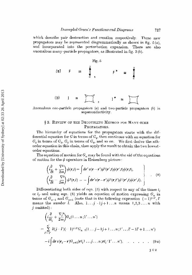
which describe pair destruction and creation respectively. These new propagators may be represented diagrammatically as shown in fig. 5 (a), and incorporated into the perturbation expansion. There are also anomalous many-particle propagators, as illustrated in fig. 5 (b).
Fig. 5
(fl) F = I - , F* I - - -
Anomalous one-particle propagators (a) and two-particle propagators (b) in superconductivity.
§ 3. REVIEW OF THE DEOOU]?LING METHOD FOl¢ MANY-TIME
PROPAGATORS.
The hierarchy of equations for the propagators starts with the dif- fcrential equation for G in terms of G 2, then continues with an equation for G 2 in terms of G 3, G3 in terms of G4, and so on. We first derive the nth- order equation in this chain, then apply the result to obtain the two lowest- order equations.
The equation of motion for G~ may be found with the aid of the equations of motion for the ¢ operators in Heisenberg picture :
f *~t + ~ ¢(r,t)-- dr'v(r-r')¢*(r',t)~h(r',t)~h(r,t),
(s) ( i ~ 2 ~ ) ~b*(r , t )=- fdr'v(r-r')¢t(r,t ')~'(v',t)¢(r',t).
Differentiating both sides of eqn. (5) with respect to any of the times tj or tj, and using eqn. (8) yields an equation of motion expressing G~ in terms of Gn_ 1 and Gn+ 1 (note that in the following expression ( - 1)J+t', l' means the number 1. Also, 1 . . . j - l j + ] . . . . n means 1,2,3 . . . . n with j omitted):
+ z m / n'
= ~, ~ ( j - l ' ) ( - 1 ) J + l ' G n _ l ( 1 . . . j - l j + l . . . n ; l ' . . . l ' - l l ' + l . . . n ' ) l ' - - V
if dr v(rj- r)G~+l(rt j l . . . j . . , n ;r t j+V.. . n'), . . . . . (9 a)
3 c 2
Dow
nloa
ded
by [
Uni
vers
ity o
f Sy
dney
] at
02:
33 2
6 A
pril
2013
728 R. D. Mat tuck and A. Theumann on
i a VJ '2~Gn(1 . . . n ; l ' . . n ' )
= - ~ 8 ( 1 - j ' ) ( - 1 ) t + J G ~ + l ( 1 . . . 1 - 1 1 + l . . n ; l ' . . . j ' - l j ' + l . . . n ' ) l = 1
+ i f d r v ( r - r / ) G ~ + l ( r t y l . . . n ; r t j , + l ' . . . j ' . . . n ' ) , . . . . (9b)
where $ ( j - 1)- ~(xj - xl) = ~ ( r j - rt)~(t j - tl). Note t ha t there are 2n al ternative equations of motion corresponding to differentiation with respect to the 2n t ime variables.
These equations m a y be wri t ten in integral form with the aid of the bare propagator, G0(1 ;1'), which satisfies the equations:
+ ~-~)G0(1 ; 1 ' ) = 5 ( 1 - 1'), . . . . . (10a)
( i ~ 1 , V l ' ~ ) G o ( 1 ; l ' ) = - ~ ( 1 - 1 ' ) , . . . . (10b)
and we find tha t
G n ( 1 . . . n ; l ' . . . n ' )
n ' = ~ Go( j ; / ' ) ( - 1 ) j + r G ~ _ l ( 1 . . . j - l j + 1 . . . n ; l ' . . . l ' - l / ' + l . . . n ' )
l ' = 1"
( l l a )
where
G n ( 1 . . . n ; l ' . . . n ' )
Go(1 ;j ')( - 1)l+YGn_l(1... l - iI + 1 . . . n ; 1 ' . . . j ' - l j ' + 1 . . . n') / = 1
ff . . . .
- i dsds 'v (s ;s )Go(s, 3 )Gn+l(S 1 . . . n ; s +1 . . . s . . . n ' ) . ( i lb )
v(s ;s ' ) -v (rs -rs ' )~( t~- t s ' ) ' } . . . . . (12) s +=rs,ts+ and ds =drsdt s.
I t should be noted tha t (11 a, b) as they s tand are not ant isymmetr ie under exchange of two pr imed or two unpr imed variables [see (6)]. How- ever, t hey m a y be ant i symmetr ized with the aid of the operators 1 j
A-- ;-! P . . . . . . ( 1 2 a )
1 A ' = ~p ~ . ( - 1)PP,
Dow
nloa
ded
by [
Uni
vers
ity o
f Sy
dney
] at
02:
33 2
6 A
pril
2013
Decoupled Green's Functions and Diagrams 729
where P is the permutatiou operator. Applying these to G~ in (11 a, b) yields
G A=A'AG~(1 . . . . n ; l ' . . . . n ) . . . . . (12b)
which is the antisymmetrized G~. For example, in the case of G~, this becomes
I t must not be supposed, however, that all G's we deal with must be antisymmetric. The exact G's must o f course be antisymmetric but c~proximate G's need not be. For example, G~ in I~PA approximation (in fig. 4, diagrams 2 + 4 + 8 + 9 . . . . ) is non-antisymmetric, since aside from diagram 2, it contains no exchange diagrams. Hence we shall work with non-antisymmetric G's as well as the symmetrized ones.
Let us now apply ( l l a , b) to obtain the two lowest-order equations. For n = l, we find two alternative equations for the one-particle propagator G in terms oI the two-particle propagator G 2 :
G(1 ;1')= Go(1 ; l ' ) - i f fd2d3v(2;3)Go(1 ;2)G2(32 ;3+1' ) , (13a)
ffd2' ;2'+3'). (13b) G(1 ;1') = G0(1
For n = 2, we obtain G~ in terms of G and G~. There are four alternative equations in this case, corresponding to differentiation with respect to tl,Q,t 1' and t2':
Continuing in this way yields an infinite set of coupled integral equations connecting successively higher-order propagators.
The usual approximation made in solving these equations is to express some higher-order propagator--say G~+l--as a sum over products of
Dow
nloa
ded
by [
Uni
vers
ity o
f Sy
dney
] at
02:
33 2
6 A
pril
2013
730
(Q)
R. D. M a t t uck a n d A. T h e u m a n n on
Fig. 6
2
( b ) = - 2'
I ' I ' ~ I '
Diagram form of the equation of motion of G in terms of G2 (see eqns. (13 a, b)).
Fig. 7 1 I 2 I 2 I 2 ,÷ , ~ ~
I ' 2' I' 2' I' 2' I' 2'
I 2 I 2 I 2 ,,. I 12
Ht-X-' I ' 2' I ' 2' I ' 2' I ' 2'
I 2 I 2 I 2 I 2
1' 2' 1' 2' 1' 2" 6', '
1 2 1 2 1 2 1 2
I ' 2' I ' 2' I ' 2'
1' 2'
Diagram form of the equation of motion for G2 in terms of G 3 (see eqns. (14 a, b, c, d)). (e) is the antisymmetrized form of (a).
Dow
nloa
ded
by [
Uni
vers
ity o
f Sy
dney
] at
02:
33 2
6 A
pril
2013
(Q)
I 2
n-1
n
I' 2'
n'
-1
n'
Fig.
8
I 2
J-1
J J+
1 n
I' 2'
J"
n"
+ (-
i) j'"
'
I 2
J-1
J J*
1 n
I' ?'
J'
n'-1
n"
t- °
oo +
I 2
J-1
J J+
1 n
1'
2'
l' n'
-2
n'-I
n'
.+.
i z
i j
S. S
~S
n
I' 2'
n' ¢b
~b
I 2
n-1
n I
2 J
n
I' Z'
n'
-1
n'
I' J'-
1 J'
J'+1
n'
I 2
n-2
n-1
n
"~
'~(
-1
)J
"n
-1
+
I' J'-
1 J'
J'*1
n'
I 2
n-1
n I
2 n
I" J'-
1 J'
J'÷1
n"
s~
Dia
gram
for
m o
f th
e eq
uati
on o
f m
otio
n fo
r G
~ in
ter
ms
of G
n+ 1
(see
eqn
s. (
11 a
, b)
and
see
jus
t af
ter
eqn.
(8)
reg
ardi
ng n
otat
ion)
.
ce
o~
¢,#
Dow
nloa
ded
by [
Uni
vers
ity o
f Sy
dney
] at
02:
33 2
6 A
pril
2013
732 t/,. D. Mattuck and A. Theumann on
lower-order ones. This decouples the pth-order equation from all the higher-order equations and we obtain just p coupled equations to be solved simultaneously for G,G2 . . . . . G~. For example, in eqn. (14a) (or 14 b, c, or d) we might set G 3 ~ G x G2, yielding an equation involving G,G2, to be solved together with eqns (13 a) or (13 b).
§ 4. DIAGIgAMMATIC REPI~ESENTATION OF THE EQUATIONS OF MOTION
To make it easier to investigate the relation between the decoupling and partial sum methods, let us first express the equations of motion for the many -time propagators in diagram form. With the aid of the diagram for G~in fig. 3 (b), the G-G~ eqns. (13a, b), may be drawn as shown in fig. 6 (a), (b), and the G2-G 3 eqns. (14a, b, c, d) have the form shown in fig. 7(a), (b), (c), (d). The antisymmetrized form of, for example fig. 7 (a), is shown in fig. 7(e) (cf. eqn. (12c)). The general eqns. ( l la , b) for the n-particle propagator G~ are shown diagrammatically in fig. 8 (a), (b).
I t can be seen from figs. 6, 7, 8, that in the first n diagrams on the right, the bare single-particle propagator always emerges at that point whose time we differentiate with respect to, e.g. tj or t:.,. In the 'fish' diagram on the extreme right, the bare propagator is always attached to the 'fin' corresponding to t i or tj.,. The interaction line always runs from the bare propagator to the 'mouth' of the fish.
§ 5. DECOUt'LED EQUATION OF MOTION EXPRESSED AS A I:)ARTIAL SUM
In this section we will show that any given decoupling of the many-time Green's function equations of motion is equivalent to a partial sum in perturbation theory. The method is simply to express the decoupling diagrammatically and iterate in the deeoupled equations of motion. This immediately generates an infinite series composed of definite types of Feynman diagrams, i.e. a partial sum. We will deal only with specific examples, but as will be apparent (see §5.6), the method is perfectly general. I t must be emphasized that we are only able to demonstrate the equivalence in one direction, e.g. decoupling-~partial sum.
Before carrying out this programme, a couple of general remarks are appropriate. First of all, comparing the Dyson eqn. (4 a) with the equation of motion (13a), or eqn. (4b) with eqn. (13b), we obtain an exact relation between the proper self-energy ~ and the two-particle propagator, G 2 :
or
f d2 = iJ d3' ;3)G2(3'1 ;3'+3). (15b) G(1 ;2)~(2 ;3) v(3 t I
The diagram form of eqns. (15a, b) is shown in fig. 9(a), (b). This equation will be useful in those eases where the decoupling leads to a partial sum producing a result having the Dyson equation form. However, as will be seen, there are many decouplings which do not yield a sum giving
Dow
nloa
ded
by [
Uni
vers
ity o
f Sy
dney
] at
02:
33 2
6 A
pril
2013
1)ecoupled Green's Functions and Diagrams 733
the Dyson form (see paragraph after eqn. (4)), so that fig. 9 (a), (b) cannot be used and we cannot identify a proper self-energy.
In those eases where a proper self-energy ~ can be identified, it turns out to contain both clothed and bare propagators, so that we have a sort of 'half self-consistent' perturbation theory (see after eqn. (4)). In the @coupling method, it is usual to make a further approximation in which the clothed propagators in ~ are replaced by bare ones, and we will in most eases make the same approximation here.
Fig. 9
3 2 1
1'
3: 3'+ 3
(a) (b) Relation between proper self-energy ~ and two particle propagator, G 2.
We go on now to give several examples of the deeoupling" of G 2 and G 3 and show the partial sums to which they are equivalent. The analysis of the deeoupling of higher-order propagators follows immediately from these.
5. l. Hartree-Fock Approximation
The lowest-order approximation for G is obtained by decoupling the G 2 appearing on the right-hand side of eqn. (13 a) as follows:
Note that this is antisymmetric. Equation (16) is shown diagrammatically in fig. 10 (a). Substituting this for the G~ appearing in fig. 6 (a), and noting that there is a ( - l) for the bubble loop, yields the self-consistent equation for G shown in fig. 10(b). This is the self-consistent Hart ree-Foek
Fig. 10
1 2 1 2 1 2
I ' 2' I' 2' I ' 2'
(Q)
(c)
1 1 1 1
1' 1' 1' 1'
(b}
= ~ +
(d) Deeoupling leading to Hartree-Fock approximation.
Dow
nloa
ded
by [
Uni
vers
ity o
f Sy
dney
] at
02:
33 2
6 A
pril
2013
734 l~. D. Mattuck and A. Theumann on
approximation. I f we replace G by G O in ~ , we obtain fig. t0 (d), which is just the ordinary Hartree-Fock or first-order approximation for ~.
5.2. Ladder A p p r o x i m a t i o n Better approximations for G may be obtained by deeoupling Ga in the
equation of motion for G 2. There are many possibilities here, since there are many ways of decoupling Ga, and there are four different G e-G 8 equations (see fig. 7) plus their antisymmetrized forms. A given decoupling together with a given equation of motion leads to a unique partial sum for G, as we will see in this and the next sections.
We first consider a combination of decoupling and G~-G 3 equation which leads to ladder approximation. Suppose we decouple G s in the form shown in fig. l 1 (a), i.e.
If this is substituted into the fish part of fig. 7 (c), we find the result in the second diagram of fig. 11 (b). This may be distorted into the third diagram of fig. 11 (b), which is topologically equivalent to (and therefore the same as) the second diagram. Substituting this result into the whole equation in fig. 7 (c) yields fig. 11 (c). Iterating fig. 11 (c) by substituting the whole right-hand side of this equation for the G~ on the right, etc., generates immediately the series for G~ shown in fig. 11 (d). Aside from the fact that some of the propagators are clothed this is just the ladder partial sum for G~, especially useful in low-density systems.
We now put the s6ries for G 2 into fig. 9 (a), yielding fig. 11 (e). Cancelling the clothed propagator from both sides produces the partial sum for the proper self-energy shown in fig. 11 (f). I t is very important to observe at this point that each proper self-energy diagram involves both bare and clothed propagators, giving us a sort of 'half self-consistent' perturbation theory. As we shall see, this seems to be a general characteristic of the partial sums produced by iterating the decoupled equations of motion. Following the usual procedure in the decoupling method, we replace G by G o in the proper self-energy diagrams, giving the final result fig. 11 (g), which is recognized as just the ladder sum for the proper self-energy.
5.3. Antisymmetrized Ladder Approximation Martin and Schwinger (1959) and Puff (1961) have used a decoupling
leading to a ladder sum, which is explicitly antisymmetric in the indices 1', 2', 3' but not in 1, 2, 3. I t is given by
This is shown diagrammatically in fig. 12 (a). This decoupling is placed in an antisymmetrized form of fig. 7 (a) in which the antisymmetrization is only with respect to the unprimed indices (i.e. fig. 7 (e), but without the last two 'galloping fish' diagrams). The result is shown in fig. 12 (b). Diagrams 1 + 5, 2 + 6, 3 + 9, 4 + 8 may be combined with the aid of fig. 6 (a). Noting that the equation is antisymmetric in 1,2, we may exchange the labels 3,4 in diagram (7). and change its sign. This yields fig. 12 (c) which is just the antisymmetrized form of the ladder equation, fig. l l (c). Iterating, placing the result in fig. 9 (a) and setting G = G o in the self-energy, we obtain exactly the same result as in fig. 11 (g).
5.4. Random-phase Approximation (Ring Diagrams) The decoupling of G a leading to a partial sum over 'ring' diagrams for
Substituting this into fig. 7 (c) yields the 'hooked fish' of fig. 13 (b), which may be iterated to give fig. 13 (c). In the case of an electron gas, the terms containing a hole bubble are cancelled by the positive charge background and may be dropped. Eliminating these terms, and putting fig. 13 (c) into
Dow
nloa
ded
by [
Uni
vers
ity o
f Sy
dney
] at
02:
33 2
6 A
pril
2013
736
(o)
R. D. Mat tuek and A. 'Theumann on
Fig. 12
I 2 3 I 2 3 I 2 3 I 2 3
1' 2' 3' r 2 '3 ' 1' 2' 3' 1' 2' 3'
(b)
1 2
-- {{ t -X + i f 4 - X - r 2' I 2 3 4
+
5 6 7
8 9 10
(c)
Deeoupling leading to antisymmetrized ladder sum.
fig. 9 (a) gives the part ial sum for the proper self-energy shown in fig. 13 (d). Sett ing G ~_ G 0, this is just the ring sum or 'RPA' .
Note t h a t it is absolutely necessary to use a n o n - a n t i s y m m e t r i e G 2,
e.g. t ha t in fig. 13 (e), to get the R P A self-energy. I f we had constructed an ant isymmetr ized version of 13 (c), and placed it in fig. 9 (a) we would find diagrams of non-ring type showing up in the series of fig. 13 (d). Tha t is, we would no longer have RPA.
To show tha t eqn. (19) corresponds to the R.P.A. deeoupling introduced by Pines (1963) in the operator equation-of-motion method, i t is necessary to express our equations in momentum space. This is shown in fig. 14. Note t ha t conservation of momen tum has been incorporated into the labelling. The G 2 on the left of fig. 14 (b) m a y be wri t ten (after two permutat ions of the operators, and dropping times for brevity) :
G~ = ( - i)U(T{Cl_q*ClCk_qCk*}} . . . . . . (20)
For k,1 above the Fermi surface and k - q,1 - q below the Fermi surface, this m a y be interpreted as the propagator of a particle-hole pair of momen tum q. Then fig. 14 (b) m a y be regarded as the equat ion of motion
Dow
nloa
ded
by [
Uni
vers
ity o
f Sy
dney
] at
02:
33 2
6 A
pril
2013
fo)
Decoupied Green's Functions and Diagrams
1 2 3
1' 2' 3'
Fig. 13 1 2 3
1' 2' 3'
737
(b) 1 2 1 2 1 2 1 2
)~ -- t~ -X- ~ , , 1' 2' 1' 2' 1" Z' 1'
(c) )~ -- tH -X+ o4~+ H+
Deeoupling leading to random phase spproximation (I~PA).
Fig. 14
k k q k
k k k
(b)
I k-q I k-q
i -q k l -q
(c)
n l k-q n [ k-q
n-p t -q ,p k n-q [ k
Equations of motion (a), (b) und RPA decoupling (c) in momentum sp~ce.
Dow
nloa
ded
by [
Uni
vers
ity o
f Sy
dney
] at
02:
33 2
6 A
pril
2013
738 g . D. Mat tuck and A. Theumann on
for such a pair, analogous to equation (3-165) of Pines (1963). Now, in the fish on the right of fig. 14 (b), there is a sum over the intermediate variable p. However, when the deeoupled G a of fig. 14 (c) is placed in the fish, conserva- t ion of momen tum requires tha t 1 - q + p = 1, so tha t we must have p = q. This is just the definition of R P A given by Pines : in the equat ion of motion of a pMr of momen tum q, only the te rm with m o m e n t u m transfer p = q should be kept. In addition, the number operator occurring in the deeoupling should be replaced by its unper turbed average value. In our case, since the average value of the number operator m a y be obtained directly from the single-particle propagator, this corresponds to replacing G by G O in the part ial sum for the proper self-energy.
5.5. Decoupled Equations of Motion which do not lead to a Dyson Equation for G
In the previous examples, it was shown how various decouplings of G a lead to a Dyson equation for G. Now we will examine two cases in which the partial sum obtained ealmot be writ ten in the Dyson form.
For example, let us decouple G a as in fig. 15 (a) and iiltroduce i t into fig. 7 (a). This leads to the integral equation in fig. 15 (b). I terat ing in 15 (b), and placing the resulting partial sum in fig. 6 (a} yields the expression
Fig. 15
(c)
A decoupling which does not lead to a Dyson equation.
Dow
nloa
ded
by [
Uni
vers
ity o
f Sy
dney
] at
02:
33 2
6 A
pril
2013
Decoupled Green's Functions and Diagrams 739
for G shown in fig. 15 (c), (d). This expression evidently does not have the Dyson form, fig. 2 (a), since the propagator leading into the proper self- energy parts included in ~ is bare, instead of clothed. This ~means that there are no repeated ~ parts. The same type of result is obtained if we deeonple in fig. 7 (b).
Another example is shown in fig. 16. We put the deeoupling shown in 16 (a) into the equation of motion in fig. 7 (d). Iterating the result and substituting in fig. 6 (a) gives fig. 16 (b) with ~ as in fig. 16 (c). Clearly this result is not of the Dyson form since it contains no repeated proper self- energy parts. Nevertheless, we may regard fig. 16 (c) as the first-order term obtained on iterating fig. 2 (a), so that it still makes some sense to talk of a proper self-energy here.
(a) (b)
(c) Another decoupling not leading to a Dyson equation.
5.6. Higher-order Decoupling
The methods used above to obtMn the partial sum corresponding to deeoupling of G~ and Ga may easily be extended to any higher-order G. By eqn. (1]a, b), G~. may be expressed in terms of G,G~_I,G~+ i. Suppose we decouple Gn+ i as a sum over products involving G,G2,G3,... Gn_l,G ~. Substituting this in the equation for G~ yields an equation of the form G~ =f(G,G 2 . . . . . G~_~,G~). Iterating in this equation yields a partial sum for G~ in terms of G,G 2 . . . . . G~_ i. We substitute this for G,~ in the eqn. (11 a, b), giving G ~ i in terms of G,G~_2,G ~. This procedure produces an equation of the form G~_i=f(G,G 2 . . . . . G~_2,G,_i) , which may be iterated to yield a partial sum for G~_ i. Going down the chain of equations in this way, we find finally the partial sum for G.
§ 6. DECOUPLTNG IN CONDENSED SYSTE1V[S
The decouplings discussed up to now apply to 'normal' or 'non-condensed' systems, and involve just ordinary propagators. But if the system has undergone a phase transition to a condensed state, then anomalous pro- pagators must also be taken into account as mentioned at the end of § 2.
Dow
nloa
ded
by [
Uni
vers
ity o
f Sy
dney
] at
02:
33 2
6 A
pril
2013
740
lol H
R. D. Mat tuck and A. T h e u m a n n on
Fig. 17
:+-d, I=-d, I=-d
- X +
- X +
(c)
Decoupling in the superconducting state.
We will briefly i l lustrate decoupling in the condensed state, using a super- conductor as an example. The anomalous propagators in this case were shown in fig. 5. The equat ions of mot ion for these propagators are p ic tured in fig. 17 (a), the lowest-order decoupling in fig. 17 (b), and the corresponding part ial sums in fig. 17 (c) (see Mat tuck and Johansson (1968)).
§ 7. DOES EVERY PARTIAL SUlK HAVE AN EQUIVALENT DECOUI~LII~G ?
We have seen t ha t it is always possible to find a par t ia l sum equivalent to any given decoupling. Is it also possible to find a decoupling equivalent to any given par t ia l sum? We feel t ha t the answer to this is NO, for the following reason. In every case we have looked at, the decoupling appears always to lead to a par t ia l sum in which half the propagators are clothed and the other hal f bare. While it is conceivable t h a t there is some sort of
Dow
nloa
ded
by [
Uni
vers
ity o
f Sy
dney
] at
02:
33 2
6 A
pril
2013
Deeoupled Green's Functions and Diagrams 741
decoupling scheme in higher order which will produce completely bare partial sums, we have been unable to find such a scheme, and suspect tha t it doesn' t exist. Tha t is, we feel tha t given a part ial sum in which all propagators are bare, there is no decoupling equivalent to it. The only way we were able to get bare partial sums at all was by introducing the extra approximat ion tha t the clothed propagators in the part ial sum should be replaced by bare ones.
We believe t ha t this s i tuat ion is general, i.e. given some arbi t rary partial sum, there is no t necessarily a deeoupling which is equivalent to it.
§ 8. TWO-TIME PROPAGATORS
Our preceding investigation has been based on the hierarchy of equations for the many- t ime propagators. An al ternative hierarchy of equations for the ' two-t ime' propagators (Zubarev 1960, Bonch-Bruevich and Tyablikov) shown in the 'squid' diagrams of fig. 18, m a y be constructed as
follows : we express the Hamil tonian in momen tum space with the inter- action term
H~= ~ V(24;13)a2ta4*ala 3 1234
and the first equation in the two-t ime hierarchy is the same as (13a), where the space integrals are now replaced by a sum over momenta . The G 2 on the right of this equat ion is of the two-t ime form :
And so on. The nth-order two-t ime propagator, G~, has the first 2 n - 1 t ime variables at t ime t, and the last one at t ime t'.
Jus t as in the many- t ime case, the usual procedure for solving the two- t ime hierarchy is to decouple by expressing some G~ (two-time) as a sum over products of lower-order two-t ime G's, for example, as in fig. 19. The question is: is this decoupling equivalent to a part ial sum? To
Fig. 19
t t t t t t t t t t
Example of deeoupling of Ga (two-time).
answer this, we might t ry to express (22) in integral form and iterate as we did in the many- t ime ease. The integral form of (22) is
As we see, this involves some quanti t ies which are no t propagators and therefore it cannot be expressed in F e y n m a n diagrams (al though other kinds of diagrams can be used (Morita 1970). Thus we cannot use the me thod of the previous sections.
However, there appears to be an al ternative procedure. First we notice t ha t since, for a t ime-independent Hamil tonian, the two-t ime propagators depend only on the t ime difference, we m a y write
a G~(t, t , t; t ' )= a G2(t,t,t;t,) (24) ~t--' - ~ . . . . .
and similarly for the higher-order propagators. Now, if the differentiation is carried out with respect to t' instead of t, we find instead of (23) an integral equat ion which can be expressed in F e y n m a n diagrams. This is shown in fig. 20 (a).
Equa l i ty (24) implies tha t the equation in fig. 20 (a) for G~ is equivalent to eqn. (23) for G 2. The precise meaning of 'equivalent ' here requires investigation, bu t we will assume t ha t it means t h a t when the same G8 is introduced on the r ight side of fig. 20 (a) an¢l on the r ight side of (23), we
Dow
nloa
ded
by [
Uni
vers
ity o
f Sy
dney
] at
02:
33 2
6 A
pril
2013
Decoupled Green's Functions and Diagrams
t t t t t
t'
Fig. 20
743
t t t t t !
t" t' t'
tl t2
(a) Integral equation for G2 (two-time) obtained from differentiation with respect to t', (b) corresponding integral equation for G2 (many-time).
obtain the same result for G~ in both cases. This is certainly t rue for the exact Gs, and should be at least approximately true for approximate G 3. We have two examples (see below) where it appears to be exact ly t rue even for approximate G 3, bu t no general proof t ha t this is always valid. Now fig. 20 (a) is just a special ease of fig. 7 (d) obtained by sett ing t 1 = t 2 -- t 1' = t and t 2' = t'. For comparison, fig. 7 (d) is also shown in fig. 20 (b). Tha t is, through use of (24), we have effectively expressed the two-t ime G2-G 3 equation of motion as a special ease of a particular m a n y t ime G~-G 3 equation of motion (namely, the one coming from differentiation with respect to the last time). This can be done in each order, the particular many- t ime equation of mot ion always being the one which has the free propagator sticking out of the 'last t ime' point, i.e. the bo t tom of the fish's
Fig. 21
(a) Decoupling of the two-time G3 in fig. 20 (a) which is topologically equivalent to that in fig. 19. (b) Corresponding decoupling of the many-time Gs.
3D2
Dow
nloa
ded
by [
Uni
vers
ity o
f Sy
dney
] at
02:
33 2
6 A
pril
2013
744 R. D. Mattuek a n d A. Theumann on
t~it in fig. 8 (b). The same argument holds for the antisymmetrie ease : we simply use the antisymmetrized version of all propagators in sight. Thus we can effectively express the two-time hierarchy of equations of motion as a special ease of a particular many-time hierarchy.
Now, any deeoupling of a two-time propagator can also be expressed as a special ease of a deeoupling of a many-time propagator. An example is shown in fig. 21. Putt, ing fig. 2t (a), (b) into fig. 20 (a), (b) respectively, we see that we have expressed the two-time deeoupled equations of motion as a speeiM ease of the many-time ones, so our previous conclusion still holds. That is, any given deeonpling of the two-time equations of motion is equivMent to a particular partial sum of Feynman diagrams.
3?he above is only a plausibility argument, since it rests on the assumption tha t when the same deeoupling of G a is introduced into fig. 20 (a) and eqn. (23), we get the same result for G~ and G. I t has been verified this is true in two special eases : Doniaeh's deeoupling of the equations of motion in the Kondo problem (Cheung and Mattuek 1970), and Nagaoka's deeoupling of these equations (Cheung Mattuek 1970, Theumann 1970). Therefore, we feel tha t it is not just idle speculation to suppose tha t the assumption is valid in general.
§ 9. CONCLUSION
We have shown that any given deeoupling of the hierarchy of equations for tile many-time propagators can be expressed as an equivalent partial sum of Feynman diagrams. This was accomplished by first expressing the equations of motion and the deeoupling in terms of Feynman diagrams, then iterating. Since there are 2n. different equations of motion in nth. order, plus the antisymmetrized forms, the partial sum obtained depeilds both on the form of the deeoupling and on the equation which is chosen in each order. Several examples of this were given.
All the partial sums we obtained were 'half self-consistent', since they always contained both clothed and bare propagators. This made it neeessatyy" to introduce the extra approximation that all propagators in the proper self-energy parts should be bare, in order to obtain such standard partiM sums as ladder and I~PA. This supported the conjecture that given a particular partial sum, it would not always be possible to find a decoupling equivalent to it.
No rigorous proof of our deeoupling-+partiM sum thesis could be offered in the ease of two-time propagators. However, by means of a 'diagram- waving argument, we were able to find a particular hierarchy of many-time equations which appeared to be equivalent to the two-time hierarchy, and this implies that since deeoupling-+partiM sum holds in the many-time ease, it must hold in the two-time ease as well.
ACKNOWI~m)G~]~NT
One of us (l~. D. Mattuek) wishes to thank Dr. G. C. Shukla for arousing his interest in this problem.
Dow
nloa
ded
by [
Uni
vers
ity o
f Sy
dney
] at
02:
33 2
6 A
pril
2013
Decoupled Green's Functions and Diagrams 745
I~EFEREI~CES
ABI~IKOSOV, A. A., GO~KOV, L. P., and DZY•LOSmNSK¥, I. E., 1963, Methods of Quantum Field Theory in Statistical Physics, translated by 1~. A. Silverman (Englewood Cliffs, New Jersey: Prentice-Hall, Inc.).
BO~cH-B~uEVlCH, V. L., and TYABLIKOV, S. V., 1962, The Green Punction Method in Statistical Mechanics (Amsterdam: North-Holland Co.).
CHEUNG, C. Y., and M~TTUCK, R. D., 1970, Phys. Rev. B, 2, 2735. DO,AN, B. G., 1967, Proc. phys. Soc., 90, 475. GLUCK, P., 1967, Proc. phys. Soc., 92, 192. KADANO~F, L. P., and BAY~, G., 1962, Quantum Statistical Mechanics (New
York: W. A. Benjamin, Irm.). KLEIn, A., 1962, Lectures on the Many Body Problem, Vol. 1, edited by E. R.
Caianello (New York: Academic Press). KOBE, D., 1966, J. math. Phys., 7, 1806. M~aTIN, P. C., and SCHWINGEa, J., 1959, Phys. Rev., 115, 1342. MATTUCK, R. D., 1967, A Guide to Feyman Diagrams in the Many Body Problem
(London: McGraw-Hill Publishing Co.). ~V[ATTUCK, l~. D., and JOKANSSON, B., 1968, Adv. Phys., 17, 509. MORITA, T., 1970, J. phys. Soc. Japan, 28, 1128. NozI~Es, P., 1964, Theory of Interacting Fermi Systems, translated by D. Hove
(New York: W. A. Benjamin, Iac.). PINES, D., 1963, Elementary Excitations in Solids (Amsterdam and New York:
W. A. Benjamin, Inc.). PUFF, 1%. D., 1961, Ann. Phys., 13, 317. SC]ZULTZ, T. D., 1964, Quantum Field Theory and the Many Body Problem
(London and New York: Gordon & Breach). THEUMX:NN, A., 1970, Physics Lett. A, 33, 204. ZUB,<REV, D. N., 1960, Soviet Phys. Usp., 3, 320.