Received: 4 November 2018 Revised: 20 May 2019 Accepted: 13 August 2019

DOI: 10.1002/asjc.2243

B R I E F PA P E R

Extended adaptive optimal control of linear systems withunknown dynamics using adaptive dynamic programming

Minggang Gan Jingang Zhao Chi Zhang

State Key Laboratory of Intelligent Controland Decision of Complex Systems, Schoolof Automation, Beijing Institute ofTechnology, Beijing, China

CorrespondenceJingang Zhao, State Key Laboratory ofIntelligent Control and Decision ofComplex Systems, School of Automation,Beijing Institute of Technology, Beijing100081, China.Email: zhaojingang521@126.com

Funding informationInternational Graduate Exchange Programof Beijing Institute of Technology;National Natural Science Foundation ofChina, Grant/Award Number: 61673065

Abstract

The extended infinite horizon optimal control problem of continuous time lin-ear systems with unknown dynamics is investigated in this paper. This optimalcontrol problem can be solved using the corresponding extended algebraic Ric-cati equation. A new policy iteration algorithm is proposed to approximate thesolution of the extended algebraic Riccati equation when the system dynamicsare known. The convergence of the proposed algorithm is proved. Based on theproposed policy iteration algorithm, an online adaptive dynamic programming(ADP) algorithm is developed to find the solution to the extended infinite hori-zon optimal control problem of unknown continuous time linear systems. Theconvergence of the online ADP algorithm is analyzed. Finally, two simulationexamples are given to demonstrate the effectiveness of the developed online ADPalgorithm.

KEYWORDSadaptive dynamic programming, continuous time, linear systems, optimal control, unknowndynamics

1 INTRODUCTION

The purpose of an optimal control problem is to find anoptimal control law that minimizes a predefined perfor-mance index function [1]. The optimal control problemhas received significant attention in past decades becauseit is not only academically challenging, but also of prac-tical significance [2,3]. This paper will mainly study theoptimal control problem of continuous time linear systemswith unknown dynamics [4,5].

According to traditional optimal control theory [1], thesolution to the infinite horizon optimal control problemof continuous time linear systems can be found by solvingthe corresponding algebraic Riccati equation. Whensystem dynamics are known, an iterative techniquehas been proposed to solve the corresponding algebraic

Riccati equation [6]. However, it is generally difficult orimpossible to model the systems accurately in practi-cal applications, such as motion systems [7], helicoptersystems [8], and wastewater treatment processes [9].Therefore, the system dynamics are usually completelyunknown or partially unknown [10–12]. The correspond-ing algebraic Riccati equation is thus extremely difficult tosolve without the precise knowledge of system dynamics.To overcome this dilemma, the model-free optimal con-trol method has been of considerable interest to the controlsystems community in recent years [13–15]. ADP is a bio-logically inspired approximate intelligent method and canhandle optimization problems with model uncertainty ormodel unknown [16–24]. For continuous time linear sys-tems, The authors of [25] propose a policy iteration-basedADP method to solve the optimal control for partially

© 2019 Chinese Automatic Control Society and John Wiley & Sons Australia, Ltd.

Asian J Control. 2019;1–10. wileyonlinelibrary.com/journal/asjc 1

2 GAN ET AL.

unknown continuous time linear systems. In [26], theauthors solve the continuous time linear systems withcompletely unknown system dynamics using an onlinepolicy iteration ADP method.

However, the performance index function in existingresults is the quadratic function of system states andcontrol inputs. They do not contain the product of sys-tem states and control inputs. In practical applications,such as mechatronic vehicle suspension systems [27] andvehicle dynamic systems [28], the product of system statesand control inputs has an important effect on its optimalcontrol design. Therefore, the extended infinite horizonoptimal control problem of continuous time linear systemswith unknown system dynamics is investigated in thispaper. The extended infinite horizon optimal controlproblem is that the performance index function containsnot only the quadratic function of system states and controlinputs, but also the product of them. Utilizing the advan-tage of ADP in model-free optimization control, thispaper will develop an online ADP algorithm to solvethe extended infinite horizon optimal control problem ofcontinuous time linear systems with unknown systemdynamics.

The main contributions of this paper are described asfollows. First, to the best of our knowledge, a new policyiteration algorithm to solve extended algebraic Riccatiequation is presented when system dynamics are known.Second, based on the proposed new policy iterativealgorithm, we develop an online ADP algorithm to solveextended infinite horizon optimal control problem ofcontinuous time linear systems. Third, the developedonline ADP algorithm does not require prior knowledgeof system dynamics. It utilizes online measured inputsand states data to achieve optimal control of the unknownsystem. This will provide a new idea to solve some prac-tical problems, such as mechatronic vehicle suspensionsystems.

The remaining sections are outlined as follows. Section2 presents the background and the problem formula-tion. In Section 3, when system dynamics are known,an iterative technique for solving the extended algebraicRiccati equation is shown. Section 4 presents an onlineADP algorithm to solve the extended algebraic Riccatiequation without requiring the prior knowledge of thesystem dynamics. Two simulation examples are given todemonstrate the effectiveness of the developed online ADPalgorithm in Section 5. Section 6 concludes this paper andgives directions for future research.

Notation: In this paper, R denotes the sets of real num-bers; || · || denotes the Euclidean norm for vectors ·; ⊗denotes the Kronecker product; vec(S) =

[sT

1 sT2 … sT

m]T ,

where S ∈ Rn×m, ss ∈ Rn (s = 1, 2, … ,m) represents thecolumns of S; In×n denotes n × n identify matrix; 𝜀 denotessmall positive number.

2 PROBLEM FORMULATION ANDPRELIMINARIES

Consider the following continuous time lineartime-invariant system

.x(t) = Ax(t) + Bu(t) (1)

where x(t) ∈ Rn×1 is the system state variables, u(t) ∈ Rm×1

is the system control input variables; system drift dynam-ics matrix A ∈ Rn×n and input matrix B ∈ Rn×m areunknown constant matrices with appropriate dimensions.For simplicity, x(t), u(t) can be abbreviated as x, u.

Different from the existing research, in this paper, theperformance index function is defined as follows

J = ∫∞

0

(xTQx + 2xTNu + uTRu

)dt (2)

where the conditions that Q = QT ≥ 0, R = RT > 0 andQ − NR−1NT ≥ 0 are satisfied.

Remark 1. Note that Equation (2) contains the productof system state variables x and control input variablesu. This is the main difference with the existing researchresults.

Assumption 1. The pair (A,B) is stabilizable.

Assumption 2. (Q − NR−1NT,A − BR−1NT) isobservable.

Problem 1. Extended infinite horizon optimal controlproblem

For the contimuous time linear optimal control problem,our objective is to find an optimal state feedback law in thefollowing form

u = −Kx (t) (3)

which minimizes the performance index function (2).Where K denotes the state feedback gain matrix.

Based on the traditional optimal control theory [1],when A and B are precisely known, the solution to thisoptimal control problem can be found by solving thefollowing extended algebraic Riccati equation

ATP + PA − (PB + N)R−1(BTP + NT) + Q = 0 (4)

Based on the conditions and assumptions mentionedabove, P* is the unique positive definite symmetric solu-tion of the extended algebraic Riccati Equation (4). Then,

GAN ET AL. 3

the optimal state feeback gian matrix K* in (3) can thus begiven by

K∗ = R−1(BTP∗ + NT) (5)

In addition, P* has the following property

J(x0;u∗) = minu

J(x0;u) = xT0 P∗x0 (6)

It is easy to see from the third item on the left side ofEquation (4) that (4) is nonlinear in P. Consequently, it isgenerally difficult to obtain P* by solving (4), especially forhigh-dimensional matrices.

When Remark 1 is not satisfied, that is N = 0, [6] hasgiven an efficient algorithm to numerically approximatethe solution of (4). Inspired by the efficient algorithm inreference [6], we will develop an iterative technique tonumerically approximate the solution of the extend alge-braic Riccati Equation (4) in this paper.

3 A NEW POLICY ITERATIONALGORITHM FOR SOLVING THEEXTENDED ALGEBRAIC RICCATIEQUATION

In this section, we firstly give the new policy iterationalgorithm by the following theorem. Next, we prove thecorrectness of the theorem

Theorem 1. K0 ∈ Rm×n is chosen such that the matrixA0 = A − BK0 is Hurwitz, and let Pk be the unique pos-itive definite symmetric solution of the linear algebraicequation

ATk Pk + PkAk + Q + KT

k RKk − KTk NT − NKk = 0 (7)

where Kk, Ak with k = 0, 1, 2, 3, … are given recursivelyby

Kk+1 = R−1(BTPk + NT) (8)

Ak = A − BKk (9)

Then, the following properties hold

(i) Ak = A − BKk is Hurwitz;(ii) P* ≤ Pk+1 ≤ Pk;

(iii) limk→∞Kk=K*,limk→∞Pk=P*.

Proof. Suppose that uk = −Kkx = −R−1BTPkx is an arbi-trary feedback law. If uk is applied to the system (1), theresulting cost (2) can be written as

J(x0;uk) = xT0 Pkx0 (10)

where Pk is defined as the cost matrix associated with thefeedback gain matrix Kk and is given as follow

Pk =

∫∞

0e(A−BKk)T t(Q + 2NKk + KT

k RKk)e(A−BKk)tdt (11)

where Pk is finite if and only if the closed loop systemmatrix A − BKk has eigenvalues with negative real parts.In this case, Pk is the unique positive definite symmetricsolution of the following linear equation [6]

(A − BKk)TPk + Pk (A − BKk) + Q + KTk RKk

− KTk NT − NKk = 0 (12)

Without loss of generality, we assume that the systemterminal time is T (where we may have T = ∞ in this case).Then, Equation (4) becomes the following finite horizonassociated Riccati equation

−.P =

ATP + PA − (PB + N)R−1(BTP + NT) + Q (13)

Substituting (8) into (13) and making some mathemat-ical transformation, we can obtain the following lineardifferential equation

.Pk =

− ATk Pk − PkAk − Q − KT

k RKk + KTk NT + NK (14)

Thus, the cost matrix Pk satisfies the linear differentialEquation (14).

Now, assume that we have a control law uk+1 = −Kk+1x.The cost matrix corresponding to the control law is Pk+1.Then, based on the previous discussion, Pk+1 satisfies thelinear differential equation

.Pk+1 = −AT

k+1Pk+1 − Pk+1Ak+1 − Q−

KTk+1RKk+1 + KT

k+1NT + NKk+1 (15)

Using the notation Ak = A − BKk, Ak+1 = A − BKk+1,and writing Ak = Ak+1 − B(Kk − Kk+1). Then substitutingAk = Ak+1 − B(Kk − Kk+1) into (15) yields

.Pk = −AT

k+1Pk − PkAk+1 − Q − KTk RKk+

(Kk − Kk+1)TBTPk + PkB(Kk − Kk+1)+

KTk NT + NKk (16)

Define 𝛿P = Pk −Pk+1, then 𝛿.P =

.Pk −

.Pk+1. Accordingly,

subtracting Equation (16) from Equation (15) yields

4 GAN ET AL.

𝛿.P = −AT

k+1𝛿.P − 𝛿

.PAk+1 − KT

k RKk + KTk+1RKk+1

(Kk − Kk+1)TBTPk + PkB(Kk − Kk+1)+

(KTk − KT

k+1)NT + N(Kk − Kk+1) (17)

Now, we add and subtract the term (Kk − Kk+1)TRKk+1 +KT

k+1R(Kk − Kk+1) from the right side of Equation (17) toobtain

𝛿.P = −AT

k+1𝛿P − 𝛿PAk+1 − (Kk − Kk+1)TR(Kk−

Kk+1) + (Kk − Kk+1)T(BTPk − RKk+1 + NT)+

(PkB − KTk+1R + N)(Kk − Kk+1) (18)

Then, the solution of Equation (18) with the boundarycondition 𝛿P = 0 is given by [29].

𝛿P = ∫T

0e(A−BKk+1)T t[(Kk − Kk+1)TR(Kk − Kk+1)−

(Kk − Kk+1)T(BTPk − RKk+1 + NT)−

(PkB − KTk+1R + N)(Kk − Kk+1)]e(A−BKk+1)tdt (19)

where T can be equal to infinity, 𝛿P = Pk − Pk+1. Then,based on Equation (8) and (19), we can obtain

𝛿P = ∫T

0e(A−BKk+1)T t[(Kk − Kk+1)TR(Kk − Kk+1)]·

e(A−BKk)tdt ≥ 0 (20)

Based on Equation (11), the cost matrix P0 associatedwith K0 is given as follow

P0(t) =

∫∞

teAT

0 (t−𝜏)(Q + 2NK0 + KT0 RK0)eA0(t−𝜏)d𝜏 (21)

Let 𝜉 = t1 − t + 𝜏, where t1 is arbitrary, we can obtain

P0(t) =

∫∞

teAT

0 (t1−𝜏)(Q + 2NK0 + KT0 RK0)eA0(t1−𝜏)d𝜏

= P0(t1) (22)

It can be seen from Equation (21) and (22) that P0(t) is aconstant matrix independent of t.

Since K0 ∈ Rm×n is chosen such that the matrix A0 =A−BK0 is Hurwitz, then ||P0(t)|| < ∞ and P0(t) satisfies (7)or (14) with k = 0. Now let K1 = R−1(BTP0 +NT), based on(20), we can obtain P1 ≤ P0. Hence P1(t) is also boundedbelow and therefore has finite norm. Thus, A1 = A−BK1 isHurwitz, and P1(t) satisfies (7) or (14) with k = 1. Similarly,

repeating the above argument for k = 2, 3, 4… … , we canobtain the desired results (i) and (ii).

According to the theorem on monotonic convergenceof positive operators in [30] there exists limk → ∞Pk =P∞. Thus, by taking the limit of (7) as k → ∞, wecan obtain

AT∞P∞ + P∞A∞ + Q + KT

∞RK∞ − KT∞NT−

NK∞ = 0 (23)

Since P* is the unique positive definite symmetric solu-tion of (23), P∞ = P∗. Based on (8), there exists lim

k→∞Kk =

K∗. Thus, we can obtain the desired result (iii).The proof of Theorem 1 is completed.

Remark 2. The linear algebraic Equation (7) is linearin Pk, one can iteratively solving Pk by (7) and recur-sively updating Kk by (8) when A and B are known.Then, the solution of the nonlinear Equation (4) is thusnumerically approximated.

Next, based on Theorem 1, we will give an offlinepolicy iteration algorithm to solve the optimal controlProblem 1.

Algorithm 1. Offline policy iteration algorithm forsolvinig the optimal control Problem 1:

Step 1: Given a stabilising feedback gain matrix K0;Step 2: Solve Pk by the following equation

(A − BKk)Tk Pk + Pk(A − BKk) + Q + KT

k RKk−KT

k NT − NKk = 0 (24)

Step 3: Solve Kk+1 by

Kk+1 = R−1(BTPk + NT) (25)

Step 4: Let k ← k + 1, if ||Pk+1 − Pk|| ≤ 𝜀 for k ≥ 0,go to Step 5; else continue Step 2 and Step 3. Where 𝜀is a predefined small threshold.Step 5: Use u = −Kk+1x as the approximated optimalcontrol input of the Problem 1.

Seen from (24) and (25), this algorithm is implementedoffline and requires the precise knowledge of the systemdynamics. However, in practice, it is often difficult to con-struct an accurate model or obtain the precise knowledgeof the system dynamics. In the next, inspired by refer-ence [11], we will develop a new online ADP algorithm tosolve Problem 1 without requiring the prior knowledge ofsystem dynamics.

GAN ET AL. 5

4 ADAPTIVE OPTIMAL CONTROLDESIGN WITHOUT SYSTEMDYNAMICS

In this section, based on the proposed new policy iterationalgorithm above, we will present an online ADP algorithmthat does not require A and B.

Assume that K0 is a known stabilizing feedback gainmatrix. To solve Equation (24), we rewrite system (1) in thefollowing form [11]

.x = Akx + B(Kkx + u) (26)

where Ak = A − BKk.Then, along the solutions of (26) by (7) and (8), one can

obtain

x(t+ ▵ t)TPkx(t+ ▵ t) − x(t)TPkx(t)

= ∫t+▵t

t[xT(AT

k Pk + PkAk)x + 2(u + Kkx)TBTPkx]d𝜏

= −∫t+▵t

txTQkxd𝜏 + 2∫

t+▵t

t(u + Kkx)TRKk+1xd𝜏

− 2∫t+▵t

t(u + Kkx)TNTxd𝜏 (27)

where Qk = Q + KTk RKk − KT

k NT − NKk.

Remark 3. It is noteworthy that in Equation (27), onecan replace the system matrices with the states andinputs data measured online. Thus, we can obtain PKand Kk+1 from Equation (27) without requiring theprecise knowledge of A and B.

Consequently, under a given stabilizing feedback gainmatrix Kk, to find (Pk,Kk+1) with the unknown systemmatrices, we introduce the Kronecker product

xTQkx = (xT ⊗ xT)vec(Qk)(Kkx + u)TRKk+1x

=[(xT ⊗ xT)(In ⊗ (Kk)TR) + (xT ⊗ uT)(In ⊗ R)

]vec(Kk+1)

(u + Kkx)TNTx = [xT ⊗ uT + (xT ⊗ xT)(ITn ⊗ KT

k )]vec(NT)

Furthermore, define the following matrices, 𝜁xx ∈ Rl×n2 ,𝛾xx ∈ Rl×n2 , 𝛾xu ∈ Rl×mn, l is a positive integer

𝜁xx =[

x ⊗ x |||t1+▵tt1

, … , x ⊗ x |||tl+▵ttl

]T

𝛾xx =[∫

t1+▵t

t1

x ⊗ xd𝜏, … ,∫tl+▵t

tl

x ⊗ xd𝜏]T

𝛾xu =[∫

t1+▵t

t1

x ⊗ u0d𝜏, … ,∫tl+▵t

tl

x ⊗ u0d𝜏]T

where 0 ≤ t1 < t2 < … < tl.

Then,Φk ∈ Rl×(n2+mn) andΨk ∈ Rl are defined as follows

Φk = [𝜁xx,−2𝛾xx(In ⊗ (Kk)TR) − 2𝛾xu(In ⊗ R)]

Ψk = −𝛾xxvec(Qk) − 2[𝛾xu + 𝛾xx(In ⊗ KTk )]vec(NT)

Therefore, Equation (27) can be rewritten in the form of alinear equation as follows

Φk

[vec(Pk)vec(Kk+1)

]= Ψk (28)

Lemma 1. Φi is a full column rank matrix, satisfyingthe following condition [16]

∃l > 0, rank([𝛾xx, 𝛾xu]) =n(n + 1)

2+ mn (29)

Lemma 2 ([7]). If K0 is a initial stabilizing feedbackcontrol gain and Lemma 1 is satisfied, the sequences{Pk}∞k=0 and {Kk}∞k=1 obtained by solving (28) will respec-tively converge to optimal P* and K*.

Now, we can give the online ADP algorithm for solv-ing the optimal control Problem 1 with unknown systemdynamics.

Algorithm 2. (Online model-free ADP algorithm)

Step 1: Initialization and online data collection: Giv-ing a stabilizing feedback gain matrix K0 and apply-ing u0 = −K0x + e as the control input t = t1 = 0,where e is the exploration noise. Compute 𝜁 xx, 𝛾xx and𝛾xu until Lemma 1 is satisfied, let k = 0.Step 2: Policy evaluation and improvement: Solve Pkand Kk+1 from Equation (28).Step 3: Let k ← k + 1, if ||Pk+1 − Pk|| ≤ 𝜀 for k ≥ 0,go to Step 4; else go to Step 2. Where 𝜀 is a predefinedsmall threshold.Step 4: Use u = −Kk+1x as the approximated optimalcontrol input of the Problem 1.

Remark 4. If A is Hurwitz, K0 can be set as K0 = 0.

5 SIMULATION RESULTS

In this section, two simulation examples are provided todemonstrate the effectiveness of the developed online ADPalgorithm.

Example 1. We consider a practical electromechani-cal vehicle suspension system described by the follow-ing two degrees of freedom of movement differentialequations [27,31]{

msxs = −ks(xs − xt) − cs(.xs −

.xt) + umtxt = ks(xs − xt) + cs(

.xs −.xt) − kt(xt − x0) − u

6 GAN ET AL.

where ms and mt are the mass of the 1/4 body and the 1/2bogie, respectively. ks and kt are the lateral stiffness of thespring. cs is damping coefficients. u is the control force. x0,xt and xs represent the displacement.

Define x1 = xs − xt, x2 = xs, x3 = xt − x0, x4 = xt, y1 = x2,y2 = x4, w = x0. Based on modern control theory, one canobtain .x = Ax + Bu + Gw

𝑦 = Cx + Duwhere x = [x1 x2 x3 x4]T denotes the state variables, y =[y1 y2]T denotes the output variables,

A =⎡⎢⎢⎢⎣

0 1 0 −1−ks∕ms −cs∕ms 0 cs∕ms0 0 0 1ks∕mt cs∕mt −kt∕mt −cs∕mt

⎤⎥⎥⎥⎦B =

[0 1∕ms 0 −1∕mt

]T

C =[−ks∕ms −cs∕ms 0 cs∕msks∕mt cs∕mt −kt∕mt −cs∕mt

]D = [∕ms − 1∕mt]T, G = [00 − 10]T

In practical applications, Gw has no effect on controlforce, so Gw can be ignored [31]. In order to improvethe smooth operation of the vehicle, while improving the

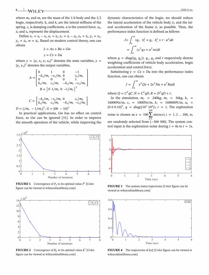
FIGURE 1 Convergence of Pk to its optimal value P* [Colorfigure can be viewed at wileyonlinelibrary.com]

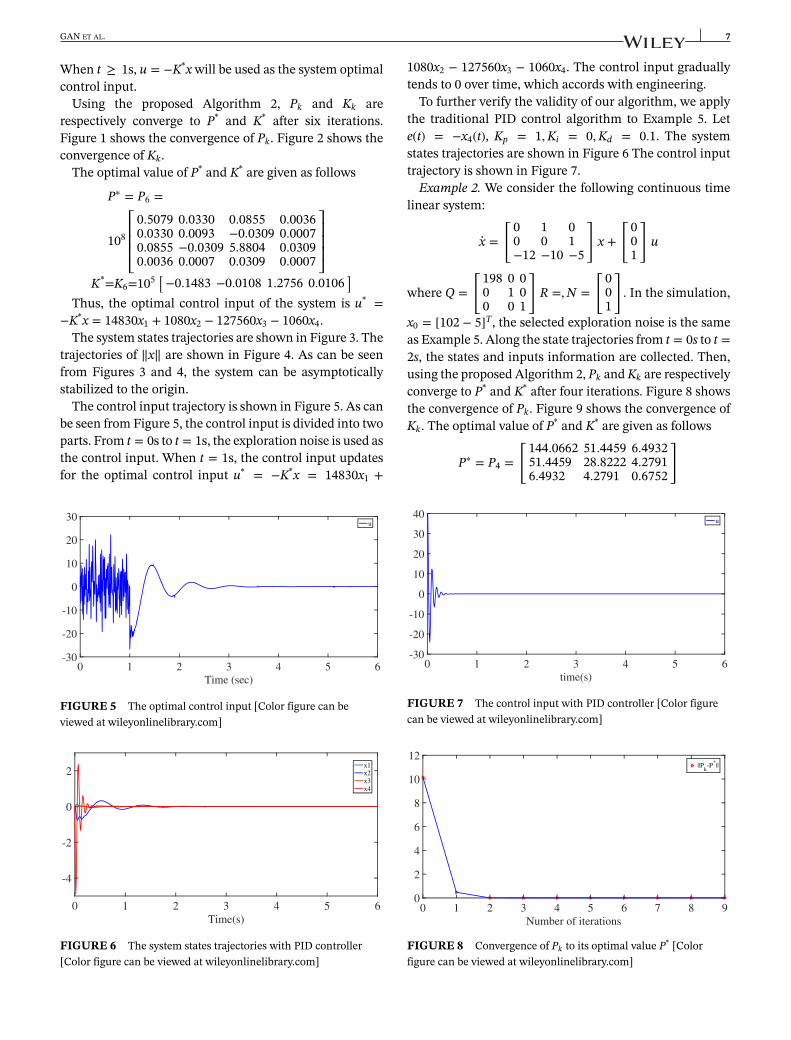
FIGURE 2 Convergence of Kk to its optimal value K* [Colorfigure can be viewed at wileyonlinelibrary.com]

dynamic characteristics of the bogie, we should reducethe lateral acceleration of the vehicle body xs and the lat-eral acceleration of the frame x t as possible. Thus, theperformance index function is defined as follows

J=∫∞

0(q1 · x2

s + q2 · x2t + r · u2)dt

= ∫∞

0(𝑦Tq𝑦 + uTru)dt

where q = diag([q1 q2]). q1, q2 and r respectively denoteweighting coefficients of vehicle body acceleration, bogieacceleration and control force.

Substituting y = Cx + Du into the performance indexfunction, one can obtain

J = ∫∞

0xTQx + 2xTNu + uTRudt

where Q = CTqC,N = CTqD,R = DTqD + r.In the simulation, ms = 240kg, mt = 36kg, ks =

16000Ns/m, cs = 1000Ns/m, kt = 160000N/m, x0 =[0 0 0.10]T, q = diag([105 104]), r = 1. The exploration

noise is chosen as e = 100100∑i=1

sin(wit), i = 1, 2… 100, wi

are randomly selected from [−500 500]. The system con-trol input is the exploration noise during t = 0s to t = 1s.

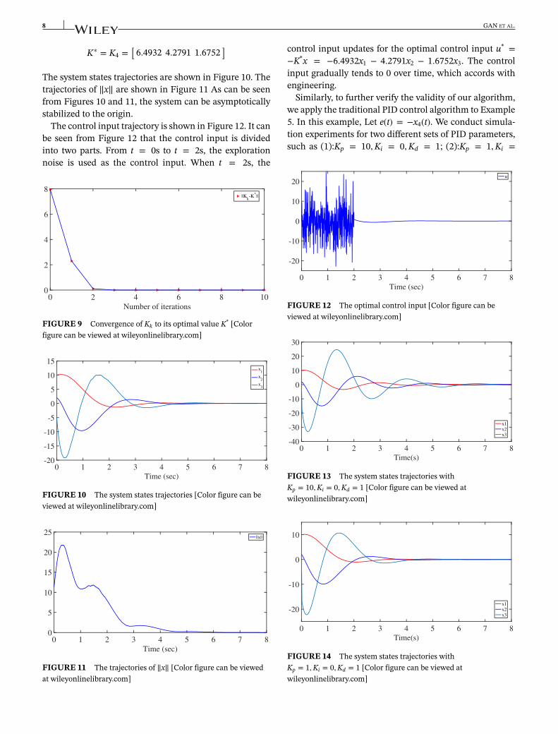
FIGURE 3 The system states trajectories [Color figure can beviewed at wileyonlinelibrary.com]

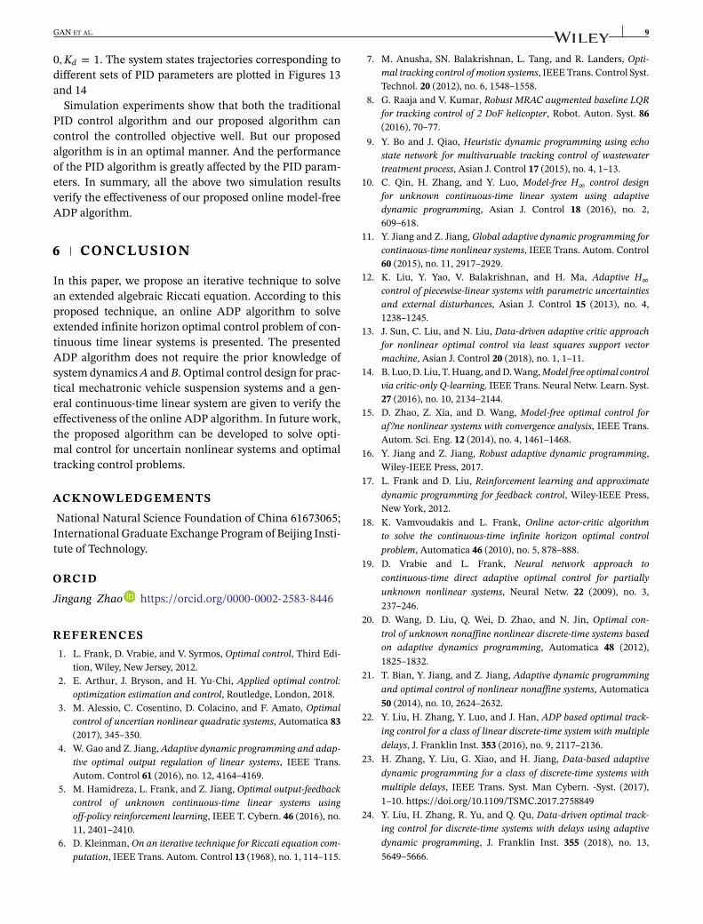
FIGURE 4 The trajectories of ||x|| [Color figure can be viewed atwileyonlinelibrary.com]

GAN ET AL. 7

When t ≥ 1s, u = −K*x will be used as the system optimalcontrol input.

Using the proposed Algorithm 2, Pk and Kk arerespectively converge to P* and K* after six iterations.Figure 1 shows the convergence of Pk. Figure 2 shows theconvergence of Kk.

The optimal value of P* and K* are given as follows

P∗ = P6 =

108

⎡⎢⎢⎢⎣0.5079 0.0330 0.0855 0.00360.0330 0.0093 −0.0309 0.00070.0855 −0.0309 5.8804 0.03090.0036 0.0007 0.0309 0.0007

⎤⎥⎥⎥⎦K*=K6=105 [−0.1483 −0.0108 1.2756 0.0106

]Thus, the optimal control input of the system is u* =

−K*x = 14830x1 + 1080x2 − 127560x3 − 1060x4.The system states trajectories are shown in Figure 3. The

trajectories of ||x|| are shown in Figure 4. As can be seenfrom Figures 3 and 4, the system can be asymptoticallystabilized to the origin.

The control input trajectory is shown in Figure 5. As canbe seen from Figure 5, the control input is divided into twoparts. From t = 0s to t = 1s, the exploration noise is used asthe control input. When t = 1s, the control input updatesfor the optimal control input u* = −K*x = 14830x1 +

FIGURE 5 The optimal control input [Color figure can beviewed at wileyonlinelibrary.com]

FIGURE 6 The system states trajectories with PID controller[Color figure can be viewed at wileyonlinelibrary.com]

1080x2 − 127560x3 − 1060x4. The control input graduallytends to 0 over time, which accords with engineering.

To further verify the validity of our algorithm, we applythe traditional PID control algorithm to Example 5. Lete(t) = −x4(t), Kp = 1,Ki = 0,Kd = 0.1. The systemstates trajectories are shown in Figure 6 The control inputtrajectory is shown in Figure 7.

Example 2. We consider the following continuous timelinear system:

.x =

[ 0 1 00 0 1−12 −10 −5

]x +

[ 001

]u

where Q =

[ 198 0 00 1 00 0 1

]R =,N =

[ 001

]. In the simulation,

x0 = [102 − 5]T, the selected exploration noise is the sameas Example 5. Along the state trajectories from t = 0s to t =2s, the states and inputs information are collected. Then,using the proposed Algorithm 2, Pk and Kk are respectivelyconverge to P* and K* after four iterations. Figure 8 showsthe convergence of Pk. Figure 9 shows the convergence ofKk. The optimal value of P* and K* are given as follows

P∗ = P4 =

[ 144.0662 51.4459 6.493251.4459 28.8222 4.27916.4932 4.2791 0.6752

]

FIGURE 7 The control input with PID controller [Color figurecan be viewed at wileyonlinelibrary.com]

FIGURE 8 Convergence of Pk to its optimal value P* [Colorfigure can be viewed at wileyonlinelibrary.com]

8 GAN ET AL.

K∗ = K4 =[

6.4932 4.2791 1.6752]

The system states trajectories are shown in Figure 10. Thetrajectories of ||x|| are shown in Figure 11 As can be seenfrom Figures 10 and 11, the system can be asymptoticallystabilized to the origin.

The control input trajectory is shown in Figure 12. It canbe seen from Figure 12 that the control input is dividedinto two parts. From t = 0s to t = 2s, the explorationnoise is used as the control input. When t = 2s, the

FIGURE 9 Convergence of Kk to its optimal value K* [Colorfigure can be viewed at wileyonlinelibrary.com]

FIGURE 10 The system states trajectories [Color figure can beviewed at wileyonlinelibrary.com]

FIGURE 11 The trajectories of ||x|| [Color figure can be viewedat wileyonlinelibrary.com]

control input updates for the optimal control input u* =−K*x = −6.4932x1 − 4.2791x2 − 1.6752x3. The controlinput gradually tends to 0 over time, which accords withengineering.

Similarly, to further verify the validity of our algorithm,we apply the traditional PID control algorithm to Example5. In this example, Let e(t) = −x4(t). We conduct simula-tion experiments for two different sets of PID parameters,such as (1):Kp = 10,Ki = 0,Kd = 1; (2):Kp = 1,Ki =

FIGURE 12 The optimal control input [Color figure can beviewed at wileyonlinelibrary.com]

FIGURE 13 The system states trajectories withKp = 10,Ki = 0,Kd = 1 [Color figure can be viewed atwileyonlinelibrary.com]

FIGURE 14 The system states trajectories withKp = 1,Ki = 0,Kd = 1 [Color figure can be viewed atwileyonlinelibrary.com]

GAN ET AL. 9

0,Kd = 1. The system states trajectories corresponding todifferent sets of PID parameters are plotted in Figures 13and 14

Simulation experiments show that both the traditionalPID control algorithm and our proposed algorithm cancontrol the controlled objective well. But our proposedalgorithm is in an optimal manner. And the performanceof the PID algorithm is greatly affected by the PID param-eters. In summary, all the above two simulation resultsverify the effectiveness of our proposed online model-freeADP algorithm.

6 CONCLUSION

In this paper, we propose an iterative technique to solvean extended algebraic Riccati equation. According to thisproposed technique, an online ADP algorithm to solveextended infinite horizon optimal control problem of con-tinuous time linear systems is presented. The presentedADP algorithm does not require the prior knowledge ofsystem dynamics A and B. Optimal control design for prac-tical mechatronic vehicle suspension systems and a gen-eral continuous-time linear system are given to verify theeffectiveness of the online ADP algorithm. In future work,the proposed algorithm can be developed to solve opti-mal control for uncertain nonlinear systems and optimaltracking control problems.

ACKNOWLEDGEMENTS

National Natural Science Foundation of China 61673065;International Graduate Exchange Program of Beijing Insti-tute of Technology.

ORCID

Jingang Zhao https://orcid.org/0000-0002-2583-8446

REFERENCES1. L. Frank, D. Vrabie, and V. Syrmos, Optimal control, Third Edi-

tion, Wiley, New Jersey, 2012.2. E. Arthur, J. Bryson, and H. Yu-Chi, Applied optimal control:

optimization estimation and control, Routledge, London, 2018.3. M. Alessio, C. Cosentino, D. Colacino, and F. Amato, Optimal

control of uncertian nonlinear quadratic systems, Automatica 83(2017), 345–350.

4. W. Gao and Z. Jiang, Adaptive dynamic programming and adap-tive optimal output regulation of linear systems, IEEE Trans.Autom. Control 61 (2016), no. 12, 4164–4169.

5. M. Hamidreza, L. Frank, and Z. Jiang, Optimal output-feedbackcontrol of unknown continuous-time linear systems usingoff-policy reinforcement learning, IEEE T. Cybern. 46 (2016), no.11, 2401–2410.

6. D. Kleinman, On an iterative technique for Riccati equation com-putation, IEEE Trans. Autom. Control 13 (1968), no. 1, 114–115.

7. M. Anusha, SN. Balakrishnan, L. Tang, and R. Landers, Opti-mal tracking control of motion systems, IEEE Trans. Control Syst.Technol. 20 (2012), no. 6, 1548–1558.

8. G. Raaja and V. Kumar, Robust MRAC augmented baseline LQRfor tracking control of 2 DoF helicopter, Robot. Auton. Syst. 86(2016), 70–77.

9. Y. Bo and J. Qiao, Heuristic dynamic programming using echostate network for multivaruable tracking control of wastewatertreatment process, Asian J. Control 17 (2015), no. 4, 1–13.

10. C. Qin, H. Zhang, and Y. Luo, Model-free H∞ control designfor unknown continuous-time linear system using adaptivedynamic programming, Asian J. Control 18 (2016), no. 2,609–618.

11. Y. Jiang and Z. Jiang, Global adaptive dynamic programming forcontinuous-time nonlinear systems, IEEE Trans. Autom. Control60 (2015), no. 11, 2917–2929.

12. K. Liu, Y. Yao, V. Balakrishnan, and H. Ma, Adaptive H∞control of piecewise-linear systems with parametric uncertaintiesand external disturbances, Asian J. Control 15 (2013), no. 4,1238–1245.

13. J. Sun, C. Liu, and N. Liu, Data-driven adaptive critic approachfor nonlinear optimal control via least squares support vectormachine, Asian J. Control 20 (2018), no. 1, 1–11.

14. B. Luo, D. Liu, T. Huang, and D. Wang, Model free optimal controlvia critic-only Q-learning, IEEE Trans. Neural Netw. Learn. Syst.27 (2016), no. 10, 2134–2144.

15. D. Zhao, Z. Xia, and D. Wang, Model-free optimal control foraf?ne nonlinear systems with convergence analysis, IEEE Trans.Autom. Sci. Eng. 12 (2014), no. 4, 1461–1468.

16. Y. Jiang and Z. Jiang, Robust adaptive dynamic programming,Wiley-IEEE Press, 2017.

17. L. Frank and D. Liu, Reinforcement learning and approximatedynamic programming for feedback control, Wiley-IEEE Press,New York, 2012.

18. K. Vamvoudakis and L. Frank, Online actor-critic algorithmto solve the continuous-time infinite horizon optimal controlproblem, Automatica 46 (2010), no. 5, 878–888.

19. D. Vrabie and L. Frank, Neural network approach tocontinuous-time direct adaptive optimal control for partiallyunknown nonlinear systems, Neural Netw. 22 (2009), no. 3,237–246.

20. D. Wang, D. Liu, Q. Wei, D. Zhao, and N. Jin, Optimal con-trol of unknown nonaffine nonlinear discrete-time systems basedon adaptive dynamics programming, Automatica 48 (2012),1825–1832.

21. T. Bian, Y. Jiang, and Z. Jiang, Adaptive dynamic programmingand optimal control of nonlinear nonaffine systems, Automatica50 (2014), no. 10, 2624–2632.

22. Y. Liu, H. Zhang, Y. Luo, and J. Han, ADP based optimal track-ing control for a class of linear discrete-time system with multipledelays, J. Franklin Inst. 353 (2016), no. 9, 2117–2136.

23. H. Zhang, Y. Liu, G. Xiao, and H. Jiang, Data-based adaptivedynamic programming for a class of discrete-time systems withmultiple delays, IEEE Trans. Syst. Man Cybern. -Syst. (2017),1–10. https://doi.org/10.1109/TSMC.2017.2758849

24. Y. Liu, H. Zhang, R. Yu, and Q. Qu, Data-driven optimal track-ing control for discrete-time systems with delays using adaptivedynamic programming, J. Franklin Inst. 355 (2018), no. 13,5649–5666.

10 GAN ET AL.

25. D. Vrabie, O. Pastravanu, M. Abu-Khalaf, and L. Frank,Adaptive opptimal control for continuous-time linear sys-tems based on policy iteration, Automatica 45 (2009), no. 2,477–484.

26. Y. Jiang and Z. Jiang, Computational adaptive optimal controlfor continuous-time linear systems with completely unknowndynamics, Automatica 48 (2012), no. 10, 2699–2704.

27. A. Unger, F. Schimmack, B. Lohmann, and R. Schwarz, Appli-cation of LQ-based semi-active suspension control in a vehicle,Control Eng. Practice 21 (2013), no. 12, 1841–1850.

28. N. Giorgetti, A. Bemporad, H. Tseng, and D. Hrovat, Hybridmodel predictive control application towards optimal semi-activesuspension, Int J. Control 79 (2007), no. 5, 521–533.

29. D. Kleinman. (1967). Suboptimal design of linear regulator sys-tems subject to computer storage limitations, Ph.D, Thesis, MIT.

30. L. Kantorovich and G. Akilov, Functional analysis in normedspaces, Macmillan, New York, 1964.

31. H. Aleksander, Optimal linear preview control of active suspen-sion, Veh. Syst. Dyn. 21 (1992), 167–195.

How to cite this article: Gan M, Zhao J, Zhang C.Extended adaptive optimal control of linear sys-tems with unknown dynamics using adaptivedynamic programming. Asian J Control. 2019;1–10.https://doi.org/10.1002/asjc.2243