INTERNATIONAL JOURNAL FOR NUMERICAL METHODS IN ENGINEERINGInt. J. Numer. Meth. Engng (2011)Published online in Wiley Online Library (wileyonlinelibrary.com). DOI: 10.1002/nme.3277
Extended isogeometric analysis for simulation of stationary andpropagating cracks
Received 22 December 2010; Revised 25 June 2011; Accepted 4 July 2011
KEY WORDS: crack; enrichment functions; extended finite element method (XFEM); extendedisogeometric analysis (XIGA); isogeometric analysis (IGA); NURBS; partition of unitymethod
1. INTRODUCTION
The study of various modes of failure, including cracking, is vitally important to guarantee the per-formance and safety of many engineering structures. Accordingly, the prediction and analysis ofcracks have been an active research topic for the computational community in general, and for thefinite element experts in particular. Despite outstanding achievements of the FEM for the anal-ysis of various engineering problems, it suffers from a number of drawbacks in the simulationof discontinuous and/or singular problems, such as crack analysis As a result, a new generationof numerical methods have been developed, including meshfree methods such as the elementfreeGalerkin method [1], reproducing kernel particle method [2], meshless local Petrov–Galerkin [3]and the extended FEM (XFEM) [4]. One of the main features of these methods is their capabilityin the analysis of moving discontinuous problems such as crack propagation, without remeshing orrearranging of the nodal points.
The isogeometric analysis (IGA) recently proposed by Hughes et al. [5] has been increasinglyand successfully used in a number of engineering problems [6], including damage and fracture
*Correspondence to: Soheil Mohammadi, School of Civil Engineering, University of Tehran, Tehran, Iran.†E-mail: [email protected]
mechanics [7, 8]. Verhoosel et al. [8] applied IGA for the analysis of cohesive cracks by modelingdiscontinuities by means of knot insertion. They also discretized the cohesive zone formulation.In this method, the reparameterization process should be performed in each step of crack growth.IGA is based on the application of a nonuniform rational B-splines (NURBS) basis function forboth the solution field approximation and the geometric description. Simple and systematic refine-ment strategies, an exact representation of common and complex engineering shapes, robustnessand higher accuracy are among the main superiorities of the method in comparison with theconventional FEM.
The possibility of enhancing IGA to simulate crack propagation problems without remeshingmakes it a suitable candidate for modeling discontinuous problems. Recently, Benson et al. [9]discussed the combination of XFEM with isogeometric analysis as a potential capability of a gen-eralized finite element formulation to illustrate that the generalized element formulation is notrestricted to spline-based analysis. Their proposed XFEM formulation is based on the weightedenrichment function [10] that allows having a blending region between the enriched and unen-riched zones. In this method, each node may not use all the available enrichment functions [9].Their weighted XFEM method has been applied in the generalized element framework and hasonly been used for linear fracture analysis of mode I fixed cracks. Further details of the methodwere reported in De Luycker et al. [11] who analyzed a fixed mode I crack with different waysof enrichment and imposition of displacement boundary conditions to achieve an optimal rate ofconvergence. In addition, another work was recently published by Haasemann et al. [12] on thecombination of quadratic NURBS functions and XFEM for the analysis of a bimaterial body with acurved interface.
The present work extends the conventional IGA to an enriched IGA approach, called eXtended-IsoGeometric Analysis (XIGA), for mixed mode fracture analysis of fixed and propagating cracks.For this purpose the superior concepts of XFEM are used to extrinsically enrich the IGA controlpoints with Heaviside and crack tip enrichment functions. As a result the entire crack can be rep-resented independent of the mesh, because the element boundaries need not be aligned to cracksurfaces remeshing is necessary. Also, the crack tip enrichment functions improve the solutionaccuracy by enhancing the description of singular stress fields near the crack tip.
This paper is organized as follows: The framework of isogeometric analysis particularly howto deal with point load and essential boundary conditions is discussed in Section 2. Then inSection 3, crack modeling and applying extrinsic enrichment functions in IGA are describedand the formulation of the proposed approach is presented. Subsequently, several numerical sim-ulations are illustrated in Section 4 to demonstrate the robustness and efficacy of the presentmethod in the analysis of crack stability and propagation. Finally, concluding remarks are presentedin Section 5.
2. ISOGEOMETRIC ANALYSIS
2.1. Basis function
The B-spline and NURBS functions are briefly discussed in this section. For more details, referto [13].
XIGA FOR SIMULATION OF STATIONARY AND PROPAGATING CRACKS
where˚Rpi
�are the NURBS functions fTig D
�Xi1 ,Xi2
�are the coordinate position of a set of
i D 1, 2, : : : ,n control points, fwig are the corresponding weights and Ni ,p are the B-spline basisfunctions of order p, which are defined in a parametric space of the so-called knot vector „.
„D˚�1, �2, : : : , �nCpC1
��i 6 �iC1, i D 1, 2, : : : ,nC p , (3)
where the knots f�ig , .i D 1, 2, : : : ,nC pC 1/ are real numbers representing the coordinates in theparametric space Œ0, 1�. In the isogeometric analysis, a particular knot vector called open knot vectorwhere the end knots are repeated p C 1 times, is utilized to satisfy the Kronecker delta property atthe boundary points [14].
B-spline basis functions are defined in the following recursive form [13]
Ni ,0.�/D
�1 if �i 6 � 6 �iCi0 otherwise
(4)
Ni ,p.�/D� � �i
�iCp � �iNi ,p�1.�/C
�iCpC1 � �
�iCpC1 � �iC1NiC1,p�1.�/ for p D 1, 2, 3, : : : (5)
Derivatives of the B-spline basis function can be computed from
dNi ,p.�/
d�D
p
�iCp � �iNi ,p�1.�/C
p
�iCpC1 � �iC1NiC1,p�1.�/ (6)
A NURBS surface of order p in �1 direction and order q in �2 direction is defined in the form of
S.�1, �2/DnXiD1
mXjD1
Ni ,p.�i /Mj ,q.�2/wi ,jnXOiD1
mXOjD1
NOi ,p.�1/M Oj ,q.�2/wOi , Oj
„ ƒ‚ …Rp,qi ,j .�1,�2/
Ti ,j 06 �1, �2 6 1 (7)
where fwi ,j g are the weights, fTi ,j g represent an n � m bidirectional control net, and fNi ,pg andfMj ,qg are the B-spline basis functions defined on the knot vectors „1 and „2, respectively.
A NURBS has the following important features:
1. NURBS basis functions form a partition of unityPniD1Ri ,p.�/D 1 8� .
2. NURBS guarantee p � 1 continuous derivatives if the internal knots are not repeated whereasit only produces Cp�k continuity if a knot has multiplicity k.
3. The support of each Rpi .�/ is compact and contained in the interval Œ�i , �iCpC1�.
In a two-dimensional case, for a given knot span (element) there are only .p C 1/ � .q C 1/number of nonzero basis functions. Therefore, the total number of control points per element isnen D .pC 1/� .qC 1/.
2.2. Isogeometric discretization
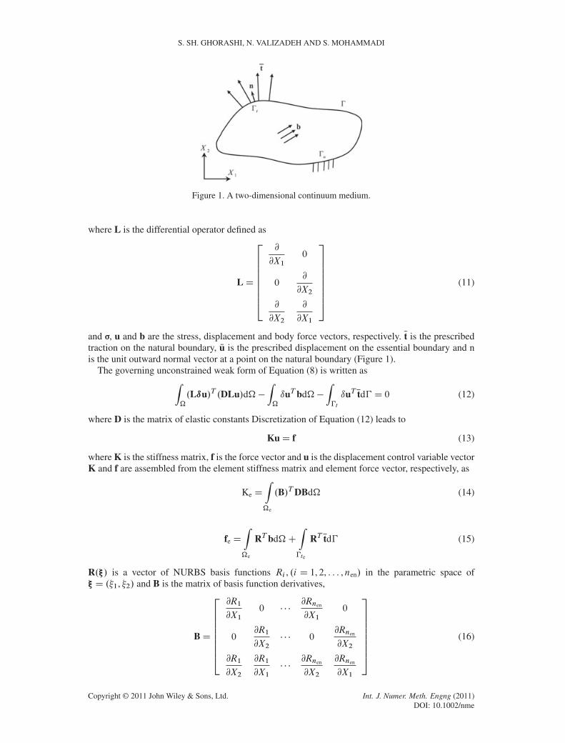
Consider a two-dimensional linear elasticity problem, as shown in Figure 1. The strong form andboundary conditions for this problem can be written as
and ¢, u and b are the stress, displacement and body force vectors, respectively. Nt is the prescribedtraction on the natural boundary, Nu is the prescribed displacement on the essential boundary and nis the unit outward normal vector at a point on the natural boundary (Figure 1).
The governing unconstrained weak form of Equation (8) is written asZ�
.Lıu/T .DLu/d��Z�
ıuT bd��Z�t
ıuT td� D 0 (12)
where D is the matrix of elastic constants Discretization of Equation (12) leads to
KuD f (13)
where K is the stiffness matrix, f is the force vector and u is the displacement control variable vectorK and f are assembled from the element stiffness matrix and element force vector, respectively, as
Ke D
Z�e
.B/TDBd� (14)
fe D
Z�e
RT bd�CZ�te
RT td� (15)
R.Ÿ/ is a vector of NURBS basis functions Ri , .i D 1, 2, : : : ,nen/ in the parametric space ofŸD .�1, �2/ and B is the matrix of basis function derivatives,
XIGA FOR SIMULATION OF STATIONARY AND PROPAGATING CRACKS
where nen D .pC 1/� .qC 1/ is the number of nonzero basis functions for a given knot span (ele-ment). Finally, the displacement approximation uh and physical coordinates XD .X1,X2/ for atypical point ŸD .�1, �2/ (parametric coordinates) can be derived from the following equations:
uh.Ÿ/DnenXiD1
Ri .Ÿ/ui (17)
X.Ÿ/DnenXiD1
Ri .Ÿ/Ti (18)
where ui is the i-th component of the vector u, derived from the solution of Equation (13). Itis observed that the NURBS basis is used for both the parameterization of the geometry and theapproximation of the solution field uh.
The derivative of the basis functions with respect to the physical coordinates in Equation (16) canbe calculated from 8̂̂<
ˆ̂:@Ri
@X1
@Ri
@X2
9>>=>>;D J�1
8̂̂<ˆ̂:@Ri
@�1
@Ri
@�2
9>>=>>; , (19)
where the Jacobian matrix J for transformation between physical and parametric spaces is defined as
JD
2664@X1
@�1
@X2
@�1
@X1
@�2
@X2
@�2
3775 . (20)
In contrast to finite elements, a control point does not generally coincide with an element vertexin the physical space.
Finally, strain and stress components can be retrieved from the approximated displacements uh
Because the NURBS basis functions do not satisfy the Kronecker delta property a direct imposi-tion of inhomogeneous essential boundary conditions to the NURBS control points may lead tosignificant errors with deteriorated rates of convergence [15].
Several methods have been developed to impose essential boundary conditions effectively, suchas the Lagrange multiplier method [1], the penalty method [16] the Nitsche’s method [17] and thereproducing kernel nodal interpolation method [18].
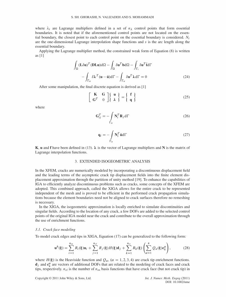
In this study, the Lagrange multiplier method is adopted for imposition of essential boundaryconditions. This method introduces a new unknown vector field œh
where �i are Lagrange multipliers defined in a set of n� control points that form essentialboundaries. It is noted that if the aforementioned control points are not located on the essen-tial boundary, the closest point to each control point on the essential boundary is considered. Niare the one-dimensional Lagrange interpolation shape functions and s is the arc length along theessential boundary.
Applying the Lagrange multiplier method, the constrained weak form of Equation (8) is writtenas [1] Z
�
.Lıu/T .DLu/d��Z�
ıuT bd��Z�t
ıuT td�
�
Z�u
ıœT .u� Nu/d� �Z�u
ıuTœd� D 0 (24)
After some manipulation, the final discrete equation is derived as [1]�K G
GT 0
��u�
�D
�fq
�(25)
where
GTij D�
Z�u
NTi Rj d� (26)
qi D�Z�u
NTi Nud� (27)
K, u and f have been defined in (13). œ is the vector of Lagrange multipliers and N is the matrix ofLagrange interpolation functions.
3. EXTENDED ISOGEOMETRIC ANALYSIS
In the XFEM, cracks are numerically modeled by incorporating a discontinuous displacement fieldand the leading terms of the asymptotic crack tip displacement fields into the finite element dis-placement approximation through the partition of unity method [19]. To enhance the capabilities ofIGA to efficiently analyze discontinuous problems such as cracks, some concepts of the XFEM areadopted. This combined approach, called the XIGA allows for the entire crack to be representedindependent of the mesh and is proved to be efficient in the performed crack propagation simula-tions because the element boundaries need not be aligned to crack surfaces therefore no remeshingis necessary.
In the XIGA, the isogeometric approximation is locally enriched to simulate discontinuities andsingular fields. According to the location of any crack, a few DOFs are added to the selected controlpoints of the original IGA model near the crack and contribute to the overall approximation throughthe use of enrichment functions.
3.1. Crack face modeling
To model crack edges and tips in XIGA, Equation (17) can be generalized to the following form:
uh.Ÿ/DnenXiD1
Ri .Ÿ/ui CncfXjD1
Rj .Ÿ/H.Ÿ/dj CnctXkD1
Rk.Ÿ/
4X˛D1
Qa.Ÿ/c˛k
!, (28)
where H.Ÿ/ is the Heaviside function and Q˛ , .˛ D 1, 2, 3, 4/ are crack tip enrichment functions.dj and c˛
kare vectors of additional DOFs that are related to the modeling of crack faces and crack
tips, respectively. ncf is the number of nen basis functions that have crack face (but not crack tip) in
XIGA FOR SIMULATION OF STATIONARY AND PROPAGATING CRACKS
their support domain and nct is the number of nen basis functions associated with the crack tip intheir influence domain.
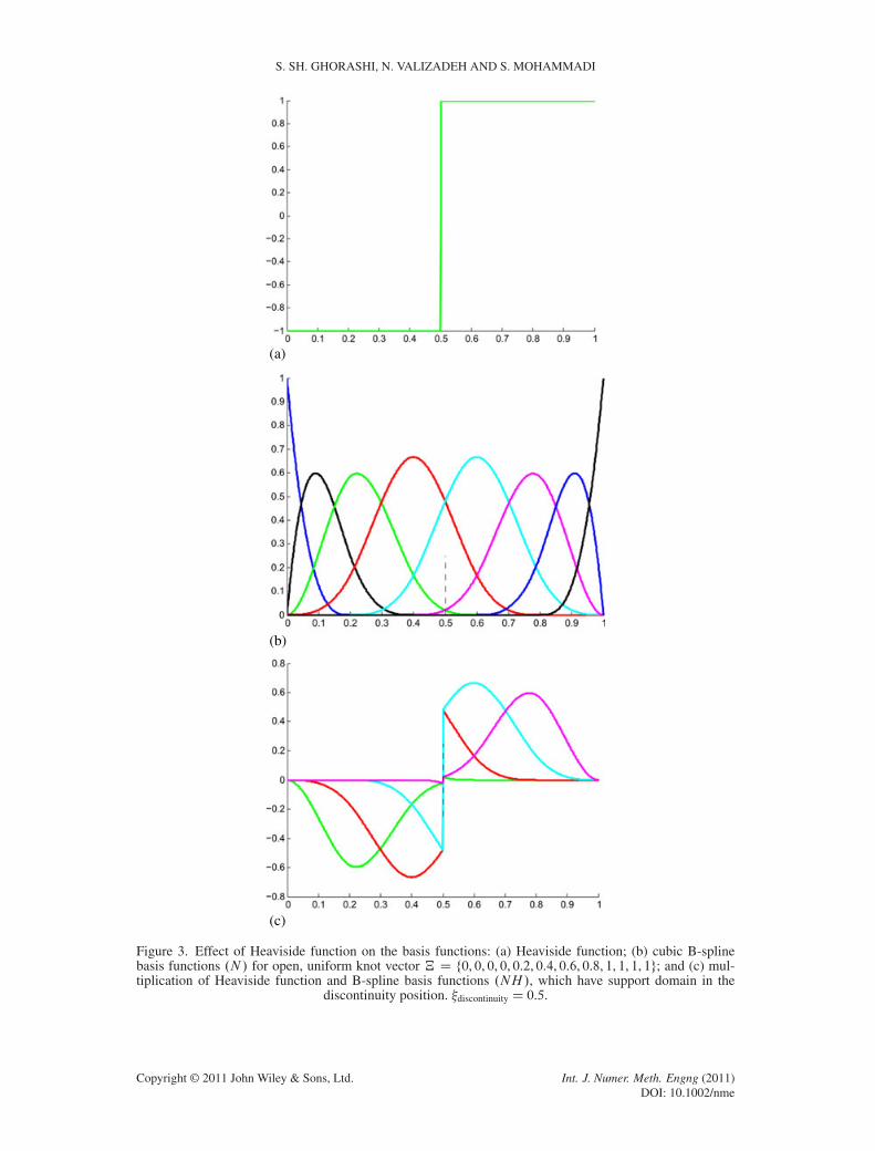
In Equation (28), H.Ÿ/ is the generalized Heaviside function [20], which otherwise becomes +1if X (physical coordinates corresponding to the parametric coordinates Ÿ) is above the crack and –1.If X� is the closest point of a crack to the point X (Figure 2) and es , en are the unit tangential andnormal vectors of the crack alignment in point X�, respectively,
H.X/D�C1 if .X�X�/ � en > 0
�1 otherwise(29)
A simple one-dimensional representation of the Heaviside function is depicted in Figure 3(a).To illustrate the effect of Heaviside function on the basis functions, an example of cubic B-splinebasis functions for an open and uniform knot vector is presented in Figure 3(b), which shows theexact interpolation of the basis functions at the ends of the interval. Elsewhere, the functions areC 2-continuous. Figure 3(c) illustrates the way the Heaviside function simulates the discontinuity.It affects the basis functions where their support domains intersect with the discontinuity location(�discontinuity D 0.5/.
3.2. Crack tip enrichment functions
The accuracy of the solution can be improved by enhancing the description of singular stress fieldsnear the crack tip through the crack tip enrichment functions. These functions span the possible dis-placement space that may occur in the analytical solution. Considering the local polar coordinatesat the crack tip .r , �/ (Figure 4), the crack tip enrichment functions are
Q.r , �/D fQ1,Q2,Q3,Q4g D
�pr sin
�
2,pr cos
�
2,pr sin � sin
�
2,pr sin � cos
�
2
�(30)
It is noted that Q1 is discontinuous along the crack face .� D�� ,�/.The local polar coordinates in the physical space are obtained in the following form:8̂<
:̂r D
qx21 C x
22
� D arctan
x2
x1
(31)
where .x1, x2/ are the local Cartesian coordinates at the crack tip Xtip D�X1tip ,X2tip
�,�
x1
x2
�D
�cos' sin'� sin' cos'
��X1 �X1tip
X2 �X2tip
�(32)
is the crack inclination angle with respect to the horizontal line at the crack tip (Figure 4) andX.Ÿ/D .X1,X2/ is defined according to Equation (18).
Figure 2. Illustration of unit tangential and normal vectors for nearest point to X on the crack surface, X�.
Figure 3. Effect of Heaviside function on the basis functions: (a) Heaviside function; (b) cubic B-splinebasis functions .N / for open, uniform knot vector „ D f0, 0, 0, 0, 0.2, 0.4, 0.6, 0.8, 1, 1, 1, 1g; and (c) mul-tiplication of Heaviside function and B-spline basis functions .NH/, which have support domain in the
XIGA FOR SIMULATION OF STATIONARY AND PROPAGATING CRACKS
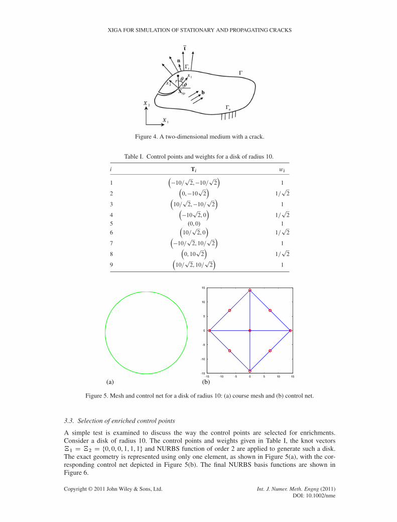
Figure 4. A two-dimensional medium with a crack.
Table I. Control points and weights for a disk of radius 10.
i Ti wi
1��10=
p2,�10=
p2�
1
2�0,�10
p2�
1=p2
3�10=p2,�10=
p2�
1
4��10p2, 0
�1=p2
5 .0, 0/ 1
6�10=p2, 0
�1=p2
7��10=
p2, 10=
p2�
1
8�0, 10p2�
1=p2
9�10=p2, 10=
p2�
1
(a) (b)
Figure 5. Mesh and control net for a disk of radius 10: (a) course mesh and (b) control net.
3.3. Selection of enriched control points
A simple test is examined to discuss the way the control points are selected for enrichments.Consider a disk of radius 10. The control points and weights given in Table I, the knot vectors„1 D „2 D f0, 0, 0, 1, 1, 1g and NURBS function of order 2 are applied to generate such a disk.The exact geometry is represented using only one element, as shown in Figure 5(a), with the cor-responding control net depicted in Figure 5(b). The final NURBS basis functions are shown inFigure 6.
Figure 6. NURBS basis functions for a disk generated by nine control points.
Figure 7. Selection of enriched control points: Tj is a Heaviside enriched control point because ofRj .Ÿc4/,Rj .Ÿc5/ ¤ 0, whereas Tk is a crack tip enriched control point because Rk.Ÿc7/,Rk.Ÿtip/ ¤ 0.
Tl is assumed an ordinary control point, because Rl .Ÿci /D 0, i D 1, 2, : : : , 7 and Rl .Ÿtip/D 0.
It is known that there is the same number of basis functions as control points. Therefore, eachbasis function can be uniquely assigned to its corresponding control point. Also, it is seen thateach basis function has its own support/influence domain and becomes zero in other points of thedomain. It is noted that because the control points may not be located in the physical space, they arenot necessarily in their basis function supports.
This feature has been used to select the crack face and crack tipenriched control points. For thispurpose, the control points that support domains of their corresponding basis functions intersectwith the crack face (not crack tip) which are enriched with the Heaviside (jump) function, while thecontrol points whose corresponding basis functions have influence domains that include the cracktip are selected to be enriched with crack tip enrichment functions. This is schematically illustratedin Figure 7, where the control points Tj and Tk are selected as the sample crack face and cracktipenriched control points, respectively. To simplify the procedure, first the parametric coordinatesof the crack tip .Ÿtip/ are calculated, then the NURBS functions of this point are obtained. Thenonzero NURBS values Ri .Ÿtip/¤ 0, i D 1, 2, : : : ,ncp specify the crack tip-enriched control points.Rk.Ÿtip/ ¤ 0 in Figure 7). In this case the enrichment domain does not remain constant whenthe order of NURBS or the sizes of elements around the crack tip change. In addition to this kind
XIGA FOR SIMULATION OF STATIONARY AND PROPAGATING CRACKS
of selection of enriched control points, sometimes called topological enrichment, one may applygeometrical enrichment [21] in which the area of enrichment remains constant in the refinementprocess or order elevation. For this type of enrichment, the control points whose correspondinginfluence domains of basis functions completely lie in the predefined constant domain surroundingthe crack tip are selected as crack tipenriched control points.
The same procedure can be applied to select the Heavisideenriched control points with the differ-ence being that the crack tip is replaced by some points on the crack face (Xc1, Xc2, : : : , Xc7 insteadof Xtip in Figure 7). It is worth noting that the control points selected for both Heaviside and cracktip enrichments are only considered as crack tipenriched control points. Accordingly, despite thefact that Rk.Ÿtip/ ¤ 0, Rk.Ÿc7/ ¤ 0 for the control point Tk in Figure 7, it is selected only as acrack tipenriched control point.
3.4. Numerical integration
The Gauss quadrature rule is applied to integrate over the XIGA elements. Because the accuracyof integration decreases significantly when there is discontinuity within the integration domain, anefficient technique should be adopted to avoid this drawback.
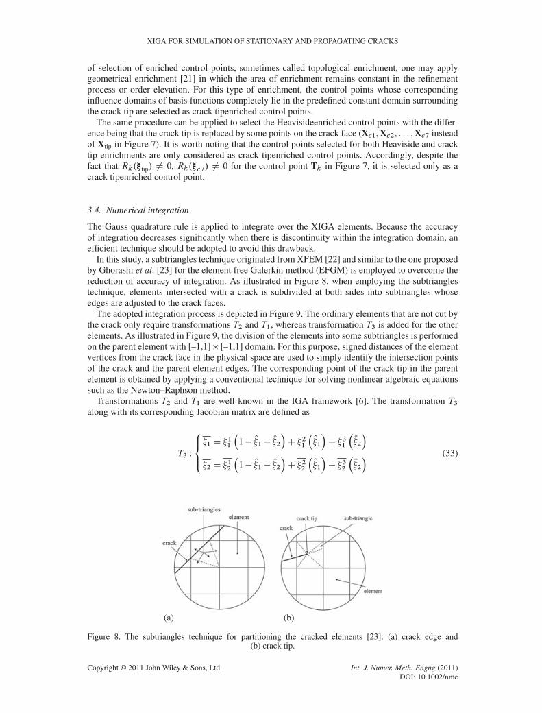
In this study, a subtriangles technique originated from XFEM [22] and similar to the one proposedby Ghorashi et al. [23] for the element free Galerkin method (EFGM) is employed to overcome thereduction of accuracy of integration. As illustrated in Figure 8, when employing the subtrianglestechnique, elements intersected with a crack is subdivided at both sides into subtriangles whoseedges are adjusted to the crack faces.
The adopted integration process is depicted in Figure 9. The ordinary elements that are not cut bythe crack only require transformations T2 and T1, whereas transformation T3 is added for the otherelements. As illustrated in Figure 9, the division of the elements into some subtriangles is performedon the parent element with [–1,1]� [–1,1] domain. For this purpose, signed distances of the elementvertices from the crack face in the physical space are used to simply identify the intersection pointsof the crack and the parent element edges. The corresponding point of the crack tip in the parentelement is obtained by applying a conventional technique for solving nonlinear algebraic equationssuch as the Newton–Raphson method.
Transformations T2 and T1 are well known in the IGA framework [6]. The transformation T3along with its corresponding Jacobian matrix are defined as
T3 W
8̂<:̂�1 D �
11
�1� O�1 � O�2
�C �21
�O�1
�C �31
�O�2
��2 D �
12
�1� O�1 � O�2
�C �22
�O�1
�C �32
�O�2
� (33)
(a) (b)
Figure 8. The subtriangles technique for partitioning the cracked elements [23]: (a) crack edge and(b) crack tip.
Figure 9. Transformations for numerical integration of a subtriangle.
Figure 10. Transformation T4 from a square into a triangle with crack tip on its vertex [24].
J3 D
266664@�1
@ O�1
@�2
@ O�1
@�1
@ O�2
@�2
@ O�2
377775D
24 ��11 C �21 ��12 C �
22
��11 C �31 ��12 C �
32
35 (34)
A more accurate integration procedure for the crack tip element can be performed by either con-sidering more subtriangles than those shown in Figure 8(b) (and Figure 9) by considering a numberof auxiliary points inside the parent element or by applying the so called ‘almost polar integration’technique proposed by Laborde et al. [24]. Application of the ‘almost polar’ technique for a cracktip element, as shown in Figure 10, requires an extra transformation T4
XIGA FOR SIMULATION OF STATIONARY AND PROPAGATING CRACKS
J4 D
266664@ O�1
@ Q�1
@ O�2
@ Q�1
@ O�1
@ Q�2
@ O�2
@ Q�2
377775D
2664
1
4
�1� Q�2
�0
1
4
��1� Q�1
� 1
2
3775 . (36)
It is obvious that the aforementioned techniques are reliable, provided that the crack path isstraight in the parametric space and in the parent element. When the crack is not straight in the para-metric space, an alternative integration process comprehensively discussed in [25], or the X-elementtechnique as discussed in [12], can be adopted for the elements cut by the crack. Nevertheless, theextension of the current methodology to curved-crack problems is an independent work in progressand is not discussed further in this paper. All the simulated numerical examples include straightcracks (or straight segments) in both physical and parametric spaces.
3.5. Extended isogeometric analysis formulation
As mentioned before, Equation (28) defines the new extrinsically enriched displacement approxi-mation for a typical point Ÿ in the proposed XIGA approach. The first term in the right-hand sideof Equation (28) is the classical IGA approximation to determine the displacement field, whilethe remaining terms are the enrichment approximation to model discontinuity and to accuratelyrepresent the analytical solution near the crack tip.
The final discretized form of the governing equation can be written as
KUD F (37)
where K is the global stiffness matrix, F is the global force vector and U is the global displacementvector that collects the displacement control variables and additional enrichment DOFs
UD fu d c1 c2 c3 c4gT (38)
K and F are assembled from the element stiffness matrix and the element force vector, respectivelyas
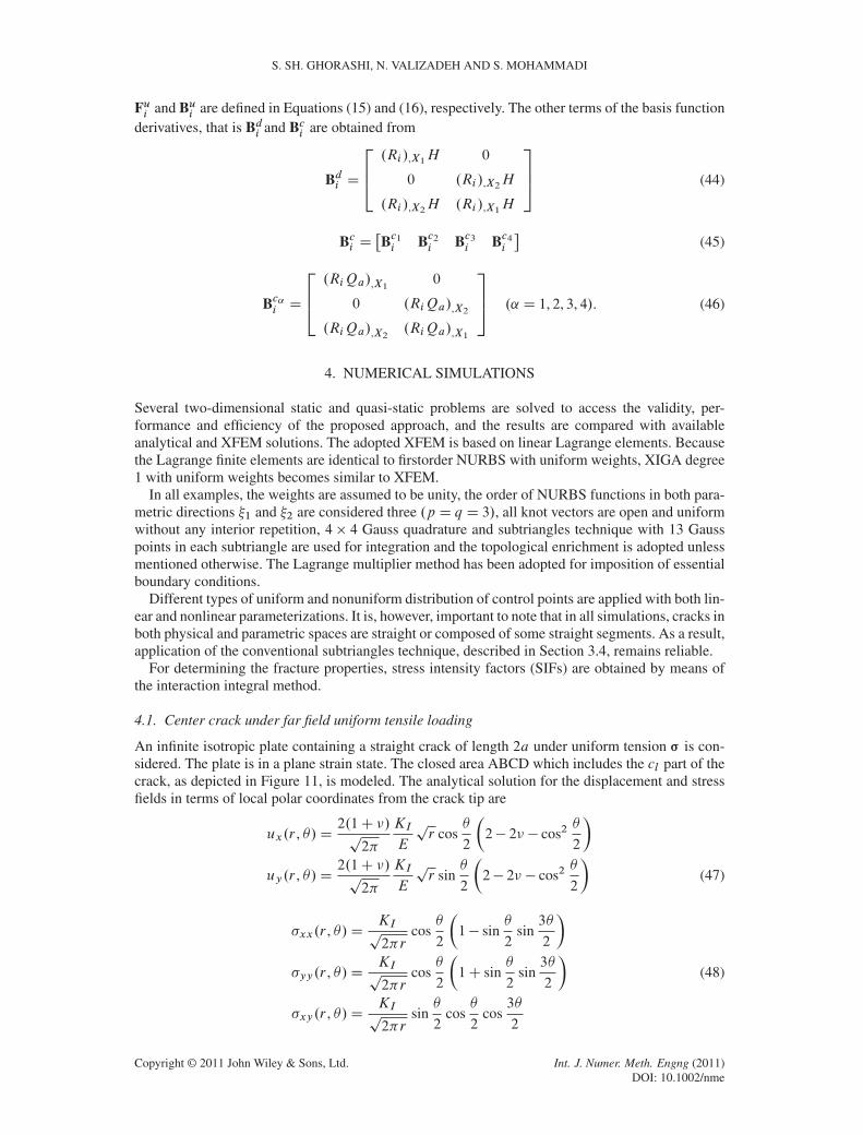
Fui and Bui are defined in Equations (15) and (16), respectively. The other terms of the basis functionderivatives, that is Bdi and Bci are obtained from
Bdi D
264.Ri /,X1H 0
0 .Ri /,X2H
.Ri /,X2H .Ri /,X1H
375 (44)
Bci D Bc1i Bc2i Bc3i Bc4i
�(45)
Bc˛i D
264.RiQa/,X1 0
0 .RiQa/,X2
.RiQa/,X2 .RiQa/,X1
375 .˛ D 1, 2, 3, 4/. (46)
4. NUMERICAL SIMULATIONS
Several two-dimensional static and quasi-static problems are solved to access the validity, per-formance and efficiency of the proposed approach, and the results are compared with availableanalytical and XFEM solutions. The adopted XFEM is based on linear Lagrange elements. Becausethe Lagrange finite elements are identical to firstorder NURBS with uniform weights, XIGA degree1 with uniform weights becomes similar to XFEM.
In all examples, the weights are assumed to be unity, the order of NURBS functions in both para-metric directions �1 and �2 are considered three .p D q D 3/, all knot vectors are open and uniformwithout any interior repetition, 4 � 4 Gauss quadrature and subtriangles technique with 13 Gausspoints in each subtriangle are used for integration and the topological enrichment is adopted unlessmentioned otherwise. The Lagrange multiplier method has been adopted for imposition of essentialboundary conditions.
Different types of uniform and nonuniform distribution of control points are applied with both lin-ear and nonlinear parameterizations. It is, however, important to note that in all simulations, cracks inboth physical and parametric spaces are straight or composed of some straight segments. As a result,application of the conventional subtriangles technique, described in Section 3.4, remains reliable.
For determining the fracture properties, stress intensity factors (SIFs) are obtained by means ofthe interaction integral method.
4.1. Center crack under far field uniform tensile loading
An infinite isotropic plate containing a straight crack of length 2a under uniform tension ¢ is con-sidered. The plate is in a plane strain state. The closed area ABCD which includes the cl part of thecrack, as depicted in Figure 11, is modeled. The analytical solution for the displacement and stressfields in terms of local polar coordinates from the crack tip are
XIGA FOR SIMULATION OF STATIONARY AND PROPAGATING CRACKS
Figure 11. Geometry and loading in a center crack plate under remote tension.
The bottom, right and top edges are considered essential boundaries and the left edge is regardedas a natural boundary, subjected to imposition of analytical solutions (47) and (48).
This problem is also analyzed by XFEM to evaluate the proposed method, with the same num-ber of field points (nodes in XFEM/control points in XIGA) and the results of both methods arecompared with the exact solution.
Three different measures of error: L2, H1 and energy errors are calculated to assess the accuracyof XIGA and XFEM
where u and uh are the exact and numerical solutions, respectively. The error norms are then reportedin a percentage form
kekkuk� 100% (55)
A variety of discretizations has been considered to measure the accuracy and convergence rate ofthe proposed approach.
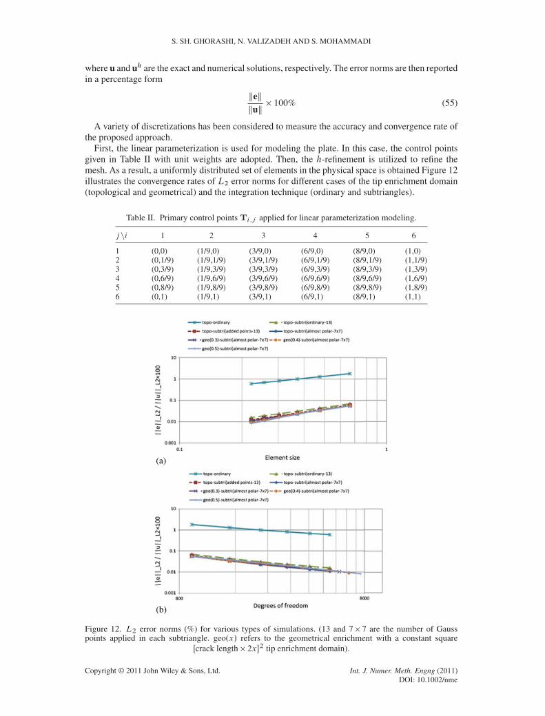
First, the linear parameterization is used for modeling the plate. In this case, the control pointsgiven in Table II with unit weights are adopted. Then, the h-refinement is utilized to refine themesh. As a result, a uniformly distributed set of elements in the physical space is obtained Figure 12illustrates the convergence rates of L2 error norms for different cases of the tip enrichment domain(topological and geometrical) and the integration technique (ordinary and subtriangles).
Table II. Primary control points Ti ,j applied for linear parameterization modeling.
Figure 12. L2 error norms (%) for various types of simulations. (13 and 7� 7 are the number of Gausspoints applied in each subtriangle. geo(x/ refers to the geometrical enrichment with a constant square
XIGA FOR SIMULATION OF STATIONARY AND PROPAGATING CRACKS
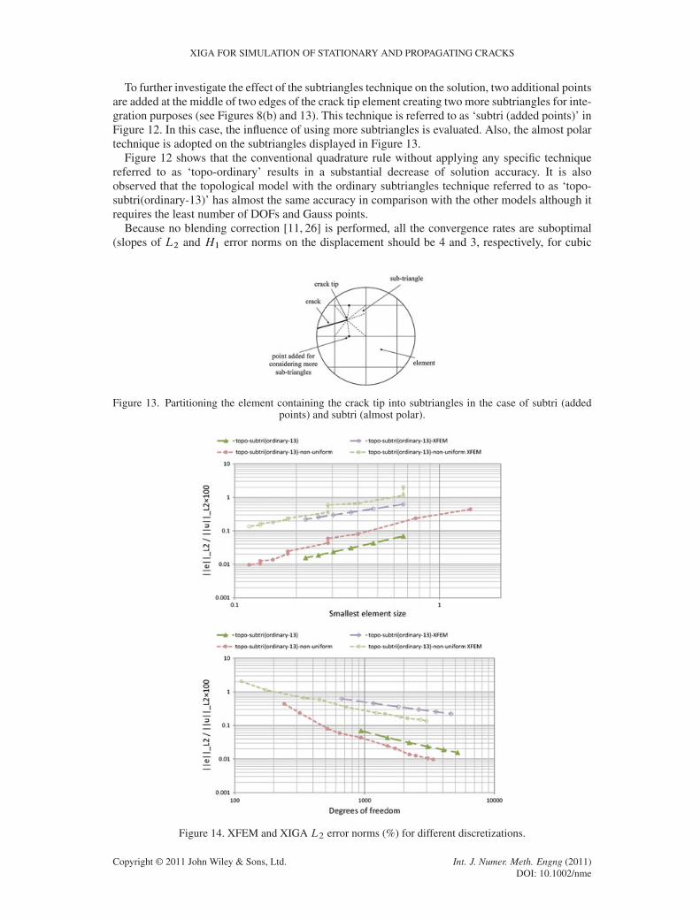
To further investigate the effect of the subtriangles technique on the solution, two additional pointsare added at the middle of two edges of the crack tip element creating two more subtriangles for inte-gration purposes (see Figures 8(b) and 13). This technique is referred to as ‘subtri (added points)’ inFigure 12. In this case, the influence of using more subtriangles is evaluated. Also, the almost polartechnique is adopted on the subtriangles displayed in Figure 13.
Figure 12 shows that the conventional quadrature rule without applying any specific techniquereferred to as ‘topo-ordinary’ results in a substantial decrease of solution accuracy. It is alsoobserved that the topological model with the ordinary subtriangles technique referred to as ‘topo-subtri(ordinary-13)’ has almost the same accuracy in comparison with the other models although itrequires the least number of DOFs and Gauss points.
Because no blending correction [11, 26] is performed, all the convergence rates are suboptimal(slopes of L2 and H1 error norms on the displacement should be 4 and 3, respectively, for cubic
Figure 13. Partitioning the element containing the crack tip into subtriangles in the case of subtri (addedpoints) and subtri (almost polar).
Figure 14. XFEM and XIGA L2 error norms (%) for different discretizations.
basis functions). Laborde et al. [24] and De Luycker et al. [11] worked on reaching optimal conver-gence rates in XFEM and isogeometric analysis combined by XFEM (for stationary cracks in modeI only), respectively.
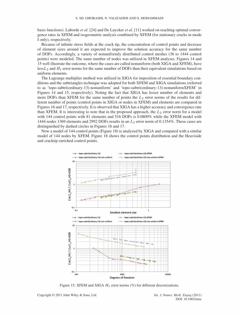
Because of infinite stress fields at the crack tip, the concentration of control points and decreaseof element sizes around it are expected to improve the solution accuracy for the same numberof DOFs. Accordingly, a variety of nonuniformly distributed control meshes (36 to 1444 controlpoints) were modeled. The same number of nodes was utilized in XFEM analyses. Figures 14 and15 well illustrate the outcome, where the cases are called nonuniform (both XIGA and XFEM), havelessL2 andH1 error norms for the same number of DOFs than their equivalent simulations based onuniform elements.
The Lagrange multiplier method was utilized in XIGA for imposition of essential boundary con-ditions and the subtriangles technique was adopted for both XFEM and XIGA simulations (referredto as ‘topo-subtri(ordinary-13)-nonuniform’ and ‘topo-subtri(ordinary-13)-nonuniformXFEM’ inFigures 14 and 15, respectively). Noting the fact that XIGA has lesser number of elements andmore DOFs than XFEM for the same number of points the L2 error norms of the results for dif-ferent number of points (control points in XIGA or nodes in XFEM) and elements are compared inFigures 16 and 17, respectively. It is observed that XIGA has a higher accuracy and convergence ratethan XFEM. It is interesting to note that in the proposed approach, the L2 error norm for a modelwith 144 control points with 81 elements and 516 DOFs is 0.0809% while the XFEM model with1444 nodes 1369 elements and 2992 DOFs results in an L2 error norm of 0.1354%. These cases aredistinguished by dashed circles in Figures 16 and 17.
Now a model of 144 control points (Figure 18) is analyzed by XIGA and compared with a similarmodel of 144 nodes by XFEM. Figure 18 shows the control points distribution and the Heavisideand cracktip enriched control points.
Figure 15. XFEM and XIGA H1 error norms (%) for different discretizations.
XIGA FOR SIMULATION OF STATIONARY AND PROPAGATING CRACKS
Figure 16. L2 error norm for various number of control points/nodes.
Figure 17. L2 error norm for various number of elements.
crack
enriched by Heaviside function
enriched by crack-tip enrichment functions
Figure 18. Distribution of 144 nonuniform control points in the proposed approach (red cross signs repre-sent the control points enriched by cracktip enrichment functions and black star signs represent the control
points enriched by the Heaviside function).
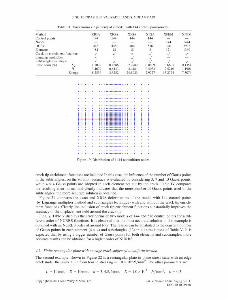
Table III compares the L2,H1 and energy norms (in percent) of XIGA and XFEM results for var-ious options of crack tip enrichments, with the imposition of essential boundaries by the Lagrangemultipliers technique and adopting the subtriangles approach for numerical integration. The distri-bution of 144 and 1444 nonuniform field points (control points in XIGA or nodes in XFEM) areshown in Figures 18 and 19, respectively.
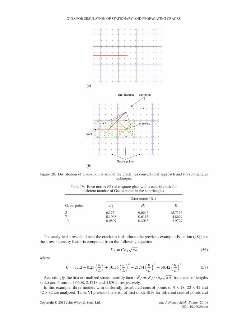
Gauss points distributions around the crack using the conventional and subtriangles techniquesare shown in Figure 20.
Table III proves the significant improvement of the proposed approach (XIGA) if used in com-bination with the Lagrange multiplier method and the subtriangles technique, where the solutionaccuracy of XIGA in a model of 144 control points and 516 DOFs is higher than the accuracy ofXFEM with 1444 nodes and 2992 DOFs. The same order of improvement is obtained when the
Energy 18.2556 3.3252 24.1923 2.9727 15.2774 7.3076
Figure 19. Distribution of 1444 nonuniform nodes.
crack tip enrichment functions are included In this case, the influence of the number of Gauss pointsin the subtriangles, on the solution accuracy is evaluated by considering 3, 7 and 13 Gauss points,while 4 � 4 Gauss points are adopted in each element not cut by the crack. Table IV comparesthe resulting error norms, and clearly indicates that the more number of Gauss points used in thesubtriangles, the more accurate solution is obtained.
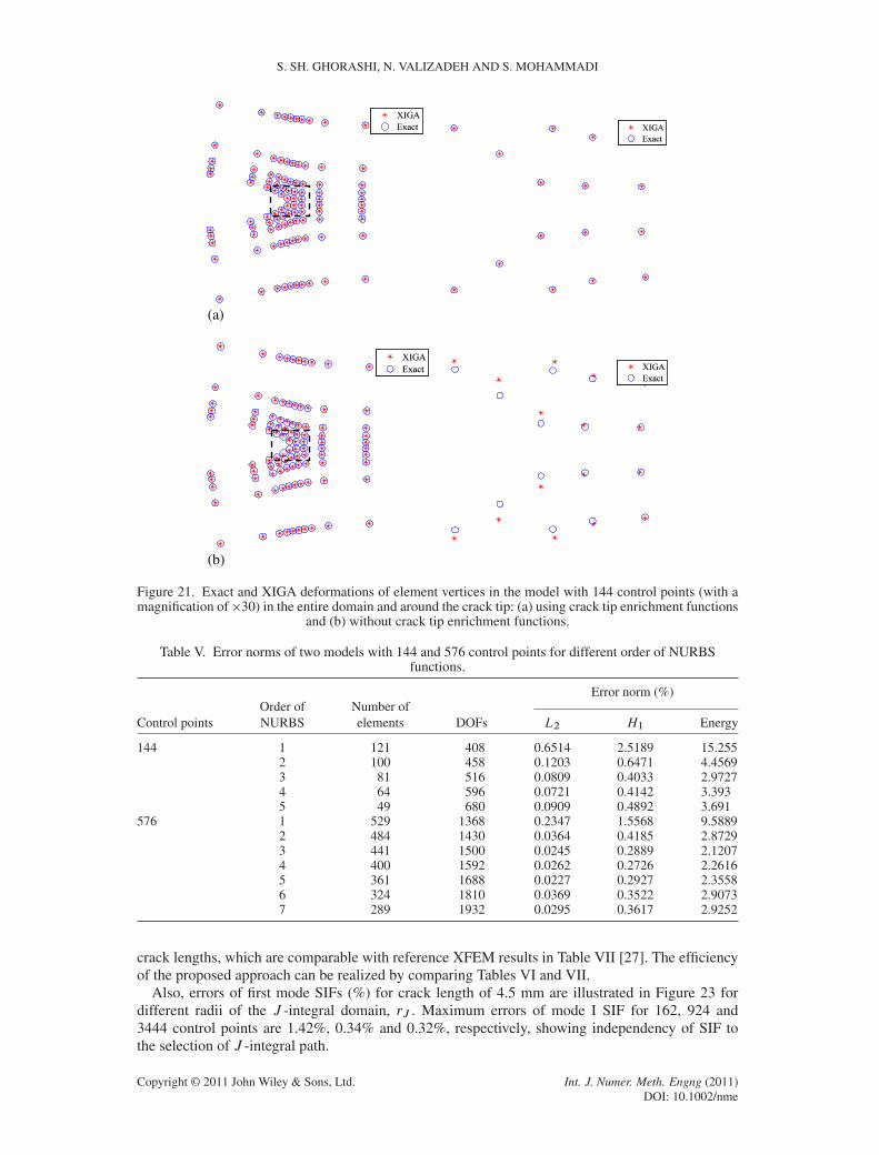
Figure 21 compares the exact and XIGA deformations of the model with 144 control points(by Lagrange multiplier method and subtriangles technique) with and without the crack tip enrich-ment functions. Clearly, the inclusion of crack tip enrichment functions substantially improves theaccuracy of the displacement field around the crack tip.
Finally, Table V displays the error norms of two models of 144 and 576 control points for a dif-ferent order of NURBS functions. It is observed that the most accurate solution in this example isobtained with an NURBS order of around four. The reason can be attributed to the constant numberof Gauss points in each element (4 � 4) and subtriangles (13) in all simulations of Table V. It isexpected that by using a bigger number of Gauss points for both elements and subtriangles, moreaccurate results can be obtained for a higher order of NURBS.
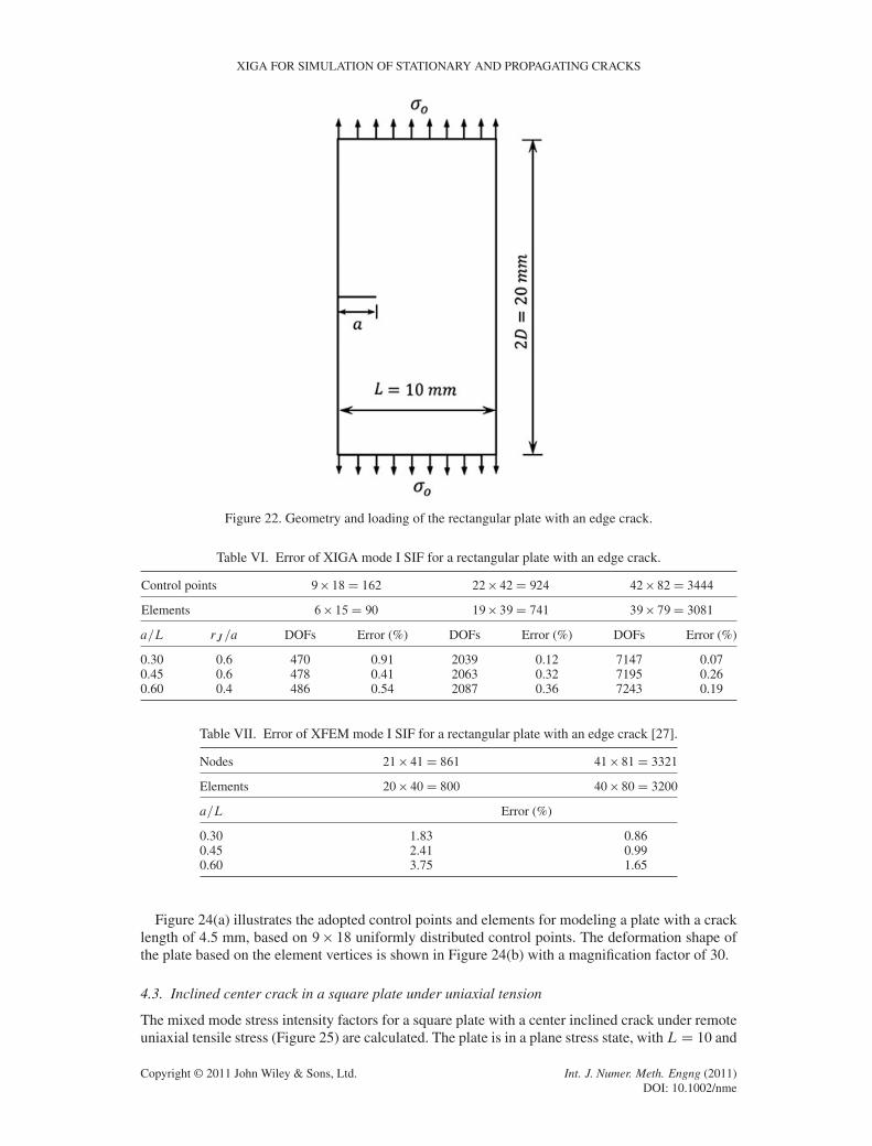
4.2. Finite rectangular plate with an edge crack subjected to uniform tension
The second example, shown in Figure 22 is a rectangular plate in plane stress state with an edgecrack under the uniaxial uniform tensile stress �0 D 1.0� 104N=mm2. The other parameters are:
LD 10mm, D D 10mm, aD 3, 4.5, 6mm, E D 1.0� 107 N=mm2, � D 0.3
The analytical stress field near the crack tip is similar to the previous example (Equation (48)) butthe stress intensity factor is computed from the following equation:
KI D C�op�a (56)
where
C D 1.12� 0.23� aL
�C 10.56
� aL
�2� 21.74
� aL
�3C 30.42
� aL
�4(57)
Accordingly, the first normalized stress intensity factor NKI DKI=��op�a�
for cracks of lengths3, 4.5 and 6 mm is 1.6608, 2.4213 and 4.0302, respectively.
In this example, three models with uniformly distributed control points of 9 � 18, 22 � 42 and42� 82 are analyzed. Table VI presents the error of first mode SIFs for different control points and
Figure 21. Exact and XIGA deformations of element vertices in the model with 144 control points (with amagnification of �30) in the entire domain and around the crack tip: (a) using crack tip enrichment functions
and (b) without crack tip enrichment functions.
Table V. Error norms of two models with 144 and 576 control points for different order of NURBSfunctions.
crack lengths, which are comparable with reference XFEM results in Table VII [27]. The efficiencyof the proposed approach can be realized by comparing Tables VI and VII.
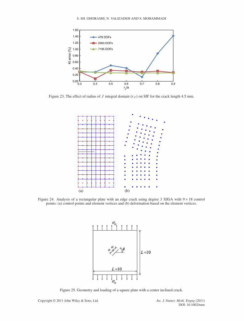
Also, errors of first mode SIFs (%) for crack length of 4.5 mm are illustrated in Figure 23 fordifferent radii of the J -integral domain, rJ . Maximum errors of mode I SIF for 162, 924 and3444 control points are 1.42%, 0.34% and 0.32%, respectively, showing independency of SIF tothe selection of J -integral path.
Table VII. Error of XFEM mode I SIF for a rectangular plate with an edge crack [27].
Nodes 21� 41D 861 41� 81D 3321
Elements 20� 40D 800 40� 80D 3200
a=L Error (%)
0.30 1.83 0.860.45 2.41 0.990.60 3.75 1.65
Figure 24(a) illustrates the adopted control points and elements for modeling a plate with a cracklength of 4.5 mm, based on 9 � 18 uniformly distributed control points. The deformation shape ofthe plate based on the element vertices is shown in Figure 24(b) with a magnification factor of 30.
4.3. Inclined center crack in a square plate under uniaxial tension
The mixed mode stress intensity factors for a square plate with a center inclined crack under remoteuniaxial tensile stress (Figure 25) are calculated. The plate is in a plane stress state, with LD 10 and
Figure 23. The effect of radius of J integral domain .rJ / on SIF for the crack length 4.5 mm.
(a) (b)
Figure 24. Analysis of a rectangular plate with an edge crack using degree 3 XIGA with 9� 18 controlpoints: (a) control points and element vertices and (b) deformation based on the element vertices.
Figure 25. Geometry and loading of a square plate with a center inclined crack.
XIGA FOR SIMULATION OF STATIONARY AND PROPAGATING CRACKS
2a D 1. Because the plate dimensions are large in comparison with the crack length, the numericalresults can be reasonably compared with the analytical solution of the infinite plate. For the knownloading �o, the exact mixed mode stress intensity factors are:
KI D �op�a cos2 , KII D �o
p�a sin cos , (58)
where is the crack inclination angle with respect to the horizontal line.As shown in Figure 26 a model of fixed nonuniform 40�40 control points with 37�37 elements
in a degree 3 XIGA is considered for analysis of the problem for various crack inclination angles.A model of 40� 40 nodes and 39� 39 elements is used in XFEM.
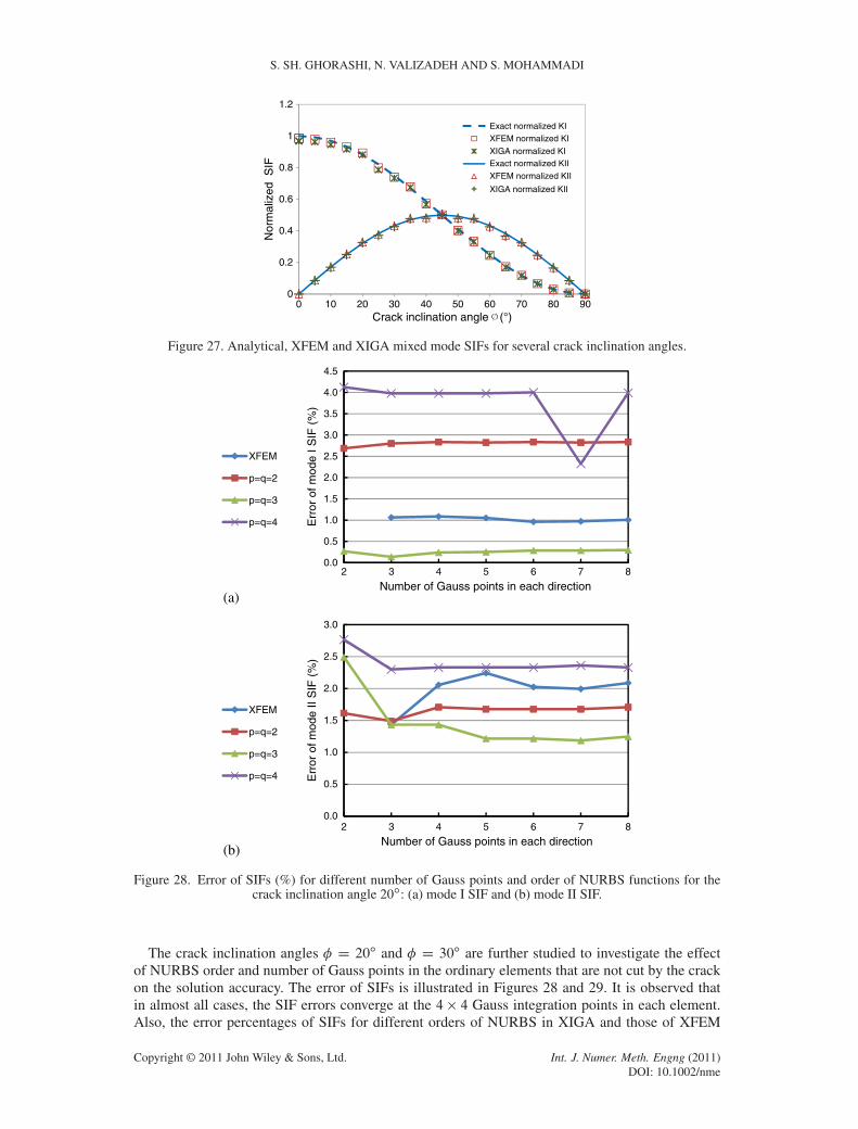
The mixed mode stress intensity factors are computed for several crack inclination angles from0ı to 90ı. The radius of the J -integral domain is assumed to be rJ D a. The XIGA, XFEM andanalytical SIFs are compared in Figure 27, which show a very close agreement.
(c)
(b)
(a)
Figure 26. Discretization of a square plate with a center inclined crack in the entire domain with its detailsaround the crack: (a) 40� 40 nonuniformly distributed control points in XIGA or nodes in XFEM; (b) 37�37
elements in XIGA; and (c) 39� 39 elements in XFEM.
Figure 27. Analytical, XFEM and XIGA mixed mode SIFs for several crack inclination angles.
0.0
0.5
1.0
1.5
2.0
2.5
3.0
3.5
4.0
4.5
2 3 4 5 6 7 8
Err
or o
f mod
e I S
IF (
%)
Number of Gauss points in each direction
XFEM
p=q=2
p=q=3
p=q=4
0.0
0.5
1.0
1.5
2.0
2.5
3.0
2 3 4 5 6 7 8
Err
or o
f mod
e II
SIF
(%
)
Number of Gauss points in each direction
XFEM
p=q=2
p=q=3
p=q=4
(a)
(b)
Figure 28. Error of SIFs (%) for different number of Gauss points and order of NURBS functions for thecrack inclination angle 20ı: (a) mode I SIF and (b) mode II SIF.
The crack inclination angles D 20ı and D 30ı are further studied to investigate the effectof NURBS order and number of Gauss points in the ordinary elements that are not cut by the crackon the solution accuracy. The error of SIFs is illustrated in Figures 28 and 29. It is observed thatin almost all cases, the SIF errors converge at the 4 � 4 Gauss integration points in each element.Also, the error percentages of SIFs for different orders of NURBS in XIGA and those of XFEM
XIGA FOR SIMULATION OF STATIONARY AND PROPAGATING CRACKS
0.0
0.5
1.0
1.5
2.0
2.5
2 3 4 5 6 7 8E
rror
of m
ode
I SIF
(%
)Number of Gauss points in each direction
XFEM
p=q=2
p=q=3
p=q=4
0.0
0.5
1.0
1.5
2.0
2.5
3.0
3.5
2 3 4 5 6 7 8
Err
or o
f mod
e II
SIF
(%
)
Number of Gauss points in each direction
XFEM
p=q=2
p=q=3
p=q=4
(a)
(b)
Figure 29. Error of SIFs (%) for different number of Gauss points and order of NURBS functions for thecrack inclination angle 30ı: (a) mode I SIF and (b) mode II SIF.
0.00
0.50
1.00
1.50
2.00
2.50
3.00
3.50
0 0.5 1 1.5 2
Err
or (
%)
J-integral radius/a
KI
KII
Figure 30. Error of SIFs (%) for different values of radius of J integral domain for the crack inclinationangle 30ı.
remain low with a maximum of about 4.12%. Because the computed SIFs slightly fluctuate for dif-ferent radius of the J -integral domain, a specific order of XIGA cannot be determined from theseresults to provide the most accurate solution. Figure 30 illustrates the error of mixed mode SIFs fordifferent values of the radius of J -integral domain for the crack inclination angle D 30ı and byconsidering a degree 3 XIGA.
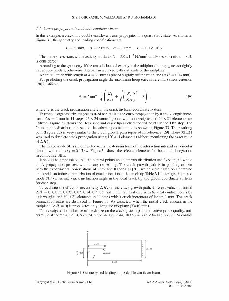
4.4. Crack propagation in a double cantilever beam
In this example, a crack in a double cantilever beam propagates in a quasi-static state. As shown inFigure 31, the geometry and loading specifications are:
LD 60mm, H D 20mm, aD 20mm, P D 1.0� 105N
The plane stress state, with elasticity modulusE D 3.0�107 N=mm2 and Poisson’s ratio D 0.3,is considered.
According to the symmetry, if the crack is located exactly in the midplane, it propagates straightlyunder pure mode I; otherwise, it grows in a curved path outwards of the midplane.
An initial crack with length of aD 20mm is placed slightly off the midplane ( H D 0.14mm/.For predicting the crack propagation angle the maximum hoop (circumferential) stress criterion
[28] is utilized
�c D 2 tan�11
4
0@ KI
KII˙
sKI
KII
2C 8
1A , (59)
where �c is the crack propagation angle in the crack tip local coordinate system.Extended isogeometric analysis is used to simulate the crack propagation by a crack length incre-
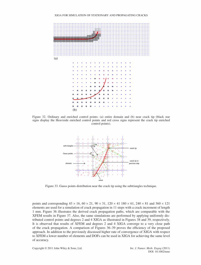
ment a D 1mm in 11 steps. 63 � 24 control points with unit weights and 60 � 21 elements areutilized. Figure 32 shows the Heaviside and crack tipenriched control points in the 11th step. TheGauss points distribution based on the subtriangles technique is shown in Figure 33. The resultingpath (Figure 32) is very similar to the crack growth path reported in reference [29] where XFEMwas used to simulate crack propagation using 120�41 elements (without mentioning the exact valueof H/.
The mixed mode SIFs are computed using the domain form of the interaction integral in a circulardomain with radius rJ D 0.15�a. Figure 34 shows the selected elements for the domain integrationin computing SIFs.
It should be emphasized that the control points and elements distribution are fixed in the wholecrack propagation process without any remeshing. The crack growth path is in good agreementwith the experimental observations of Sumi and Kagohashi [30], which were based on a centeredcrack with an induced perturbation of crack direction at the crack tip Table VIII displays the mixedmode SIF values and crack inclination angle in the local crack tip and global coordinate systemsfor each step.
To evaluate the effect of eccentricity H , on the crack growth path, different values of initial H D 0, 0.015, 0.035, 0.07, 0.14, 0.3, 0.5 and 1 mm are analyzed with 63 � 24 control points byunit weights and 60 � 21 elements in 11 steps with a crack increment of length 1 mm. The crackpropagation paths are displayed in Figure 35. As expected, when the initial crack appears in themidplane ( H D 0/ it propagates only along the midplane (Y =10 mm).
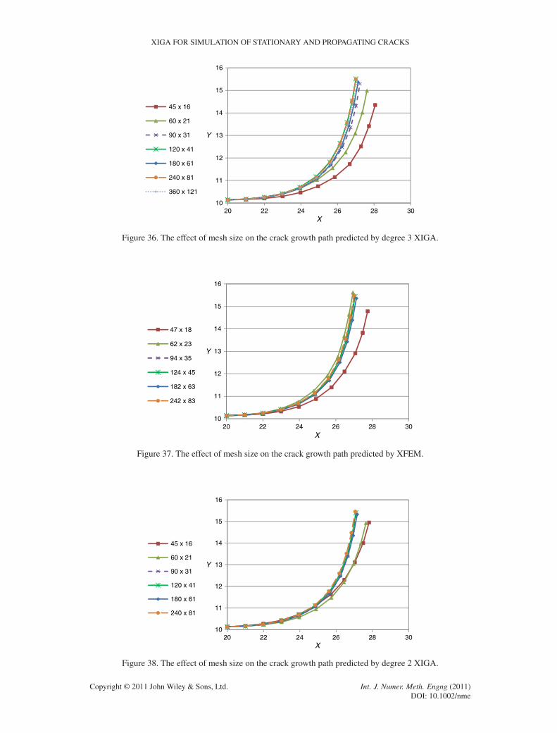
To investigate the influence of mesh size on the crack growth path and convergence quality, uni-formly distributed 48 � 19, 63 � 24, 93 � 34, 123 � 44, 183 � 64, 243 � 84 and 363 � 124 control
Figure 31. Geometry and loading of the double cantilever beam.
XIGA FOR SIMULATION OF STATIONARY AND PROPAGATING CRACKS
(a)
(b)
Figure 32. Ordinary and enriched control points: (a) entire domain and (b) near crack tip (black starsigns display the Heaviside enriched control points and red cross signs represent the crack tip enriched
control points).
Figure 33. Gauss points distribution near the crack tip using the subtriangles technique.
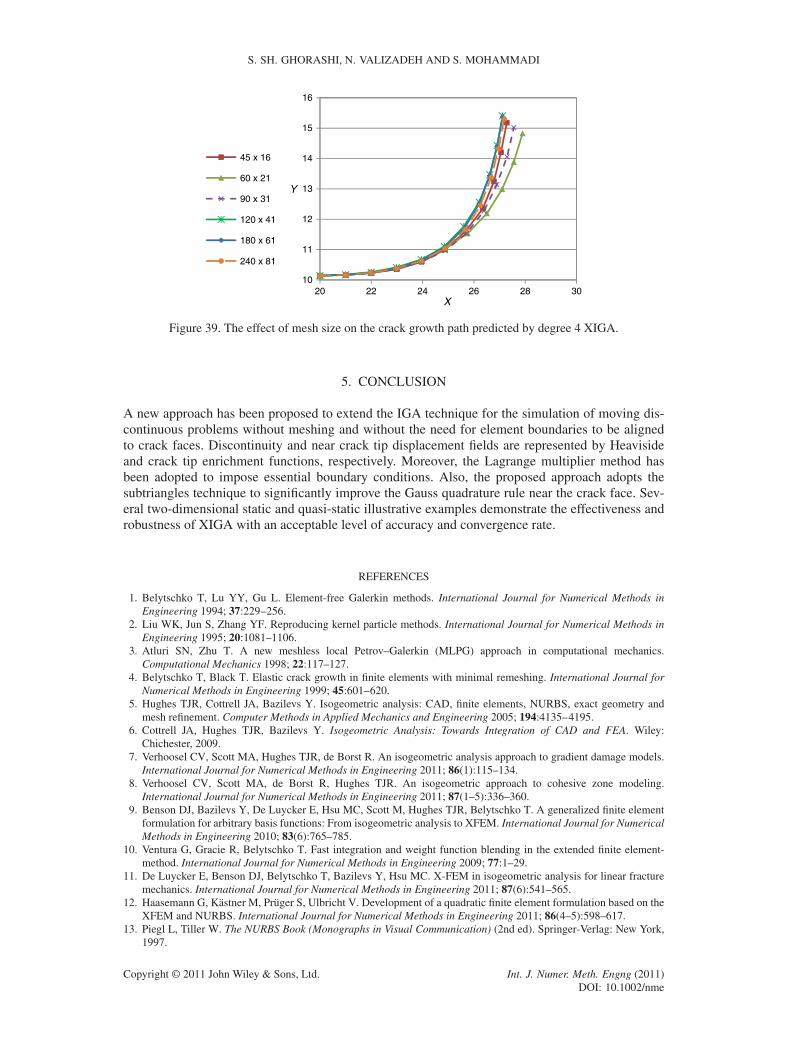
points and corresponding 45 � 16, 60 � 21, 90 � 31, 120 � 41 180 � 61, 240 � 81 and 360 � 121elements are used for a simulation of crack propagation in 11 steps with a crack increment of length1 mm. Figure 36 illustrates the derived crack propagation paths, which are comparable with theXFEM results in Figure 37. Also, the same simulations are performed by applying uniformly dis-tributed control points and degrees 2 and 4 XIGA as illustrated in Figures 38 and 39, respectively.It is observed that results of XFEM and degrees 2 and 4 XIGA converge to a very close pathof the crack propagation. A comparison of Figures 36–39 proves the efficiency of the proposedapproach. In addition to the previously discussed higher rate of convergence of XIGA with respectto XFEM a lower number of elements and DOFs can be used in XIGA for achieving the same levelof accuracy.
Figure 39. The effect of mesh size on the crack growth path predicted by degree 4 XIGA.
5. CONCLUSION
A new approach has been proposed to extend the IGA technique for the simulation of moving dis-continuous problems without meshing and without the need for element boundaries to be alignedto crack faces. Discontinuity and near crack tip displacement fields are represented by Heavisideand crack tip enrichment functions, respectively. Moreover, the Lagrange multiplier method hasbeen adopted to impose essential boundary conditions. Also, the proposed approach adopts thesubtriangles technique to significantly improve the Gauss quadrature rule near the crack face. Sev-eral two-dimensional static and quasi-static illustrative examples demonstrate the effectiveness androbustness of XIGA with an acceptable level of accuracy and convergence rate.
REFERENCES
1. Belytschko T, Lu YY, Gu L. Element-free Galerkin methods. International Journal for Numerical Methods inEngineering 1994; 37:229–256.
2. Liu WK, Jun S, Zhang YF. Reproducing kernel particle methods. International Journal for Numerical Methods inEngineering 1995; 20:1081–1106.
3. Atluri SN, Zhu T. A new meshless local Petrov–Galerkin (MLPG) approach in computational mechanics.Computational Mechanics 1998; 22:117–127.
4. Belytschko T, Black T. Elastic crack growth in finite elements with minimal remeshing. International Journal forNumerical Methods in Engineering 1999; 45:601–620.
5. Hughes TJR, Cottrell JA, Bazilevs Y. Isogeometric analysis: CAD, finite elements, NURBS, exact geometry andmesh refinement. Computer Methods in Applied Mechanics and Engineering 2005; 194:4135–4195.
6. Cottrell JA, Hughes TJR, Bazilevs Y. Isogeometric Analysis: Towards Integration of CAD and FEA. Wiley:Chichester, 2009.
7. Verhoosel CV, Scott MA, Hughes TJR, de Borst R. An isogeometric analysis approach to gradient damage models.International Journal for Numerical Methods in Engineering 2011; 86(1):115–134.
8. Verhoosel CV, Scott MA, de Borst R, Hughes TJR. An isogeometric approach to cohesive zone modeling.International Journal for Numerical Methods in Engineering 2011; 87(1–5):336–360.
9. Benson DJ, Bazilevs Y, De Luycker E, Hsu MC, Scott M, Hughes TJR, Belytschko T. A generalized finite elementformulation for arbitrary basis functions: From isogeometric analysis to XFEM. International Journal for NumericalMethods in Engineering 2010; 83(6):765–785.
10. Ventura G, Gracie R, Belytschko T. Fast integration and weight function blending in the extended finite element-method. International Journal for Numerical Methods in Engineering 2009; 77:1–29.
11. De Luycker E, Benson DJ, Belytschko T, Bazilevs Y, Hsu MC. X-FEM in isogeometric analysis for linear fracturemechanics. International Journal for Numerical Methods in Engineering 2011; 87(6):541–565.
12. Haasemann G, Kästner M, Prüger S, Ulbricht V. Development of a quadratic finite element formulation based on theXFEM and NURBS. International Journal for Numerical Methods in Engineering 2011; 86(4–5):598–617.
13. Piegl L, Tiller W. The NURBS Book (Monographs in Visual Communication) (2nd ed). Springer-Verlag: New York,1997.
XIGA FOR SIMULATION OF STATIONARY AND PROPAGATING CRACKS
14. Roh HY, Cho M. The application of geometrically exact shell elements to B-spline surfaces. Computer Methods inApplied Mechanics and Engineering 2004; 193:2261–2299.
15. Wang D, Xuan J. An improved NURBS-based isogeometric analysis with enhanced treatment of essential boundaryconditions. Computer Methods in Applied Mechanics and Engineering 2010; 199:2425–2436.
16. Zhu T, Atluri SN. A modified collocation method and a penalty formulation for enforcing the essential boundaryconditions in the element free Galerkin method. Computational Mechanics 1998; 21:211–222.
17. Fernandez-Mendez S, Huerta A. Imposing essential boundary conditions in mesh-free methods. Computer Methodsin Applied Mechanics and Engineering 2004; 193:1257–1275.
18. Chen JS, Han WM, You Y, Meng XP. A reproducing kernel method with nodal interpolation property. InternationalJournal for Numerical Methods in Engineering 2003; 56:935–960.
19. Babuška I, Melenk JM. The partition of unity method. International Journal for Numerical Methods in Engineering1997; 40(4):727–758.
20. Moës N, Dolbow J, Belytschko T. A finite element method for crack growth without remeshing. International Journalfor Numerical Methods in Engineering 1999; 46:131–150.
21. Béchet E, Minnebo H, Moës N, Burgardt B. Improved implementation and robustness study of the X-FEM for stressanalysis around cracks. International Journal for Numerical Methods in Engineering 2005; 64:1033–1056.
22. Dolbow J. An extended finite element method with discontinuous enrichment for applied mechanics. Theoretical andApplied Mechanics. Ph.D. Thesis, Northwestern University, Evanston, IL, USA, 1999.
23. Ghorashi SSh, Mohammadi S, Sabbagh-Yazdi SR. Orthotropic enriched element free Galerkin method for fractureanalysis of composites. Engineering Fracture Mechanics 2011; 78:1906–1927.
24. Laborde P, Pommier J, Renard Y, Salaün M. High-order extended finite element method for cracked domains.International Journal for Numerical Methods in Engineering 2005; 64:354–381.
25. Sevilla R, Fernández-Méndez S, Huerta A. NURBS-enhanced finite element method (NEFEM). InternationalJournal for Numerical Methods in Engineering 2008; 76(1):56–83.
26. Chessa J, Wang H, Belytschko T. On the construction of blending elements for local partition of unity enriched finiteelements. International Journal for Numerical Methods in Engineering 2003; 57:1015–1038.
27. Mohammadi S. Extended Finite Element Method for Fracture Analysis of Structures. Wiley/Blackwell: UK, 2008.28. Erdogan F, Sih GC. On the crack extension in plates under plane loading and transverse shear. Journal of Basic
Engineering 1963; 85:519–527.29. Sukumar N, Prévost JH. Modeling quasi-static crack growth with the extended finite element method. Part II:
Numerical applications. International Journal of Solids and Structures 2003; 40:7539–7552.30. Sumi Y, Kagohashi Y. A fundamental research on the growth pattern of cracks (second report). Journal of the Society
of Naval Architects of Japan 1983; 152:397–404. (in Japanese).