Extended parallelism in the Gröbner basis...

International Journal of Parallel Programming, Vol. 21, No. 1, 1992

Extended Parallelism Basis Algorithm

Stephen A. Schwab 1'2

in the Gr6bner

Received June 1991, Revised November 1992

This paper presents a new parallel implementation to compute Gr6bner bases utilizing two different forms of parallelism. A coarse-grain technique developed by Jean-Phillipe Vidal expands and reduces S-polynomials in parallel. A fine- grain technique, proposed by Melenk and Neun, constructs a pipeline of processors to overlap execution of the reduction operations. A hybrid algorithm that outperforms both of the original approaches is presented. The combined algorithm requires the user to select the appropriate allocation of processors to the two styles of parallelism, and uses this static assignment throughout the computation. The paper also discusses the design and implementation approaches used to construct an efficient version of this algorithm.

KEY WORDS: Parallel algorithms; shared memory multiprocessors; Gr6bner bases; computer algebra.

1. INTRODUCTION

Gr6bner bases are one of the basic tools of computational algebraic geometry, the branch of mathematics which, to oversimplify, studies the solutions of sets of algebraic equations in affine or projective n space. ") The significance of Gr6bner bases, which give a normal form to ideals in poly-

t The author was partially supported by an NSF graduate fellowship. This research was spon- sored in part by the Avionics Laboratory, Wright Research and Development Center, Aeronautical Systems Division (AFSC), U.S. Air Force, Wright-Patterson AFB, Ohio 45433-6543 under Contract F33615-90-C-1465, ARPA Order No. 7597 and in part by the National Science Foundation under grant CCR-87-226-33. The views and conclusions contained in this document are those of the author and should not be interpreted as representing the official policies, either expressed or implied, of the National Science Foundation or the U.S. government.

2 School of Computer Science, Carnegie Mellon University, Pittsburgh, Pennsylvannia 15213.

39

0885-7458/92/0200-0039506.50/0 �9 1992 Plenum Publishing Corporation

40 Schwab

nomial rings, as well as an algorithm for computing them, was first demonstrated by Buchberger. Once a Gr6bner basis is found for the corre- sponding ideals, it becomes easy to test if a polynomial belongs to an ideal, if two ideals are equal, if an ideal is contained in another, and so on. The interested reader is referred to Buchberger's work, (2"3) where one will find a complete introduction to Gr6bner bases, a description of their computation, as well as a list of many applications. A self-contained introduction to both the mathematical theory and applications of Gr6bner bases can also be found in the tutorial article by Misra and Yap. (4) A complete review of the various attempts to parallelize the algorithm can be found in Vidal's paper. (5)

The Buchberger algorithm transforms a set of polynomials into another set of polynomials, a Gr6bner basis generating the same ideal. These polynomials have rational coefficients, and indeterminates drawn from some finite set of variables. While the theory behind the algorithm is quite complex, the actual computation is relatively simple to describe. This implementation is based on a version of the algorithm given by Gebauer and M611erJ 6)

The computation of Gr6bner bases require a great deal of time in practice. There are several theoretical bounds but they are of limited use in predicting actual performance because they are based on worst-case complexity which is unlikely to occur in practice. One well known result is a double exponential lower-bound due to Mayr and Meyer. (7) Even when a particular instance of the problem does not require time approaching this bound, it often requires a large amount of computation. One parameterized family of examples due to Arnborg and Davenport appears to require time at least exponential in the number of equations, but this is an artificial example. Our experiments were carried out using examples from the literature, but a more useful set of measurements would require the ability to characterize and produce average case examples similar to those typically encountered when the algorithm is used, for example, in a symbolic mathematical system to solve a set of equations.

One way to speed up the solution of the problem is to transform the sequential algorithm into a parallel one and execute it on a multiprocessor. There have been many attempts over the past few years to develop an efficient parallel algorithm. Watt, ~8) and Buchberger ~9) were the first to propose parallel algorithms to compute Gr6bner bases but they did not implement them, nor attempt to measure or predict their performance. Ponder (1~ implemented corrected versions of Wart's algorithm but obtained only limited parallel speed-up. Melenk and Neun (H) designed a pipelined version of the most time consuming step of the algorithm. They simulated it and obtained good parallel efficiency for a small number of

Extended Parallelism in the Gr6bner Basis Algorithm 41

processes. More recently, Siegl (12/ modified Buchberger's parallel version of the algorithm by distributing the basis, which is a set of polynomials, among the processes. He implemented this version and obtained good performance for small examples. Senechaud (13~ had already implemented a similar version of the algorithm, but only for Boolean polynomials. Vidal (5) was the first to implement an efficient parallel algorithm on a shared memory multiprocessor.

The work presented here differs from the attempts described so far in several respects:

�9 The underlying architecture is a shared memory multiprocessor and the main objects used during the computation are shared among all processes.

�9 The implementation can be used for problems of size significantly larger than the other implementations. Also, in general, the parallel performance achieved is better than that observed in the other implementations, especially for problems of large size.

�9 This implementation is the first one which combines two parallel schemes: the coarse-grain level of parallelism similar to what Watt and Buchberger proposed is complemented by a fine-grain level of parallelism similar to what Melenk and Neun proposed. After we discuss these two parallel schemes, we will see how well both combine in one algorithm.

In Section 2, we present a brief description of the various machines on which these experiments were performed. In Section 3, we give an introduction to the Gr6bner basis algorithm. In Section 4, we present the coarse- grain parallelism of Vidal. In Section 5, we describe the fine-grain parallelism using reduction pipelines, and point out the key issues in the implementation. In Section 6, we discuss the combined version of the algorithm and the various scheduling and load balancing issues. In Section 7, we analyze the various implementations. Section 8 compares this implenta- tion to the other parallel implementations reported on in the literature. In Section 9, we conclude with a discussion of additional work and future directions.

2. M U L T I P R O C E S S O R A R C H I T E C T U R E S U S E D IN T H E I M P L E M E N T A T I O N

A wide variety of multiprocessor architectures have been described in the literature over the past few years. The characteristics of these architectures vary widely and are determined by the available technology, the class

42 Schwab

of applications addressed, the trade-offs between processor speed, memory system complexity and communication costs, and other design decisions. In this paper, we describe algorithms implemented on three shared memory architectures.

The Encore Multimax is a classic shared memory multiprocessor using a central bus for communication between processors and main memory. Each processor has a local cache and uses a snooping protocol to maintain cache coherency. The Multimax is suitable for medium and coarse grained parallel applications. (m The particular machine used in these experiments had 16 National Semiconductor 32332 processors, each rated at roughly 2 MIPS, and 32 megabytes of shared memory. The local cache size is 64K bytes, shared between two processors.

The RP3 is a large-scale research parallel processor developed at the IBM T.J. Watson Research Center. The machine consists of a number of processor-memory elements connected by an Omega-interconnection network. Local memory references are handled immediately, while remore memory references must be resolved over the network. The architecture provides three types of memory pages: local pages, global pages, and replicated pages. The machine does not support automatic cache coherency; instead, cache management is the responsibility of the program- mer or compiler. (15~ The virtual memory interface allows each page to be marked as cacheable or noncacheable, as well as allowing the cache to be flushed under user level control. The current version of the system has 64 ROMP processors. Each processor has 8 megabytes of storage, and a 64K byte local cache shared between two processors.

The Plus architecture (16) is a mesh of processor-memory elements connected by a deterministic routing network. The routers always send messages along an L-shaped path in the mesh, so that the message first propagates vertically, then horizontally to the destination. Remote memory references are transparently routed to the appropriate destination. In addition several special features enhance this basic design. Local computation proceeds while remote writes are being completed, increasing overall throughput, When needed, a fence operation is used to stall the local processor until all remote writes have completed. Also, any page in memory may be replicated to other processing nodes. Reads from these replicated pages are handled locally, while writes are directed to the master copy of the page and transparently propagated to all replicated copies. This allows the processor which owns the page to write it without stopping, while the hardware keeps track of these writes and updates the memory of other processors which have a copy of the page. Tuning an application to run on this architecture involves studying reference patterns of the algorithm and selecting a memory replication scheme that minimizes remote read refer-


ences, while limiting remote writes and overall network traffic. This type of architecture is expected to perform better than a pure message-passing architecture because additional hardware supports the remote memory references, as opposed to a software layer processing these memory requests. The experiments described in the paper were run on the Plus simulator, as well as the Proteus (~7~ simulator configured to model the Plus architecture. A machine with 40 nodes is currently under construction.

There are several key differences between these architectures that impact on how applications are tuned to these machines. The Multimax, with a uniform memory system accessed via a common bus, requires no decisions about where to locate data structures in the machine. Both the RP3 and Plus support nonuniform memory systems, so data locality is critical to performance. Synchronization on the Multimax uses a test-and- set primitive, which requires exclusive access to the bus, making this a potentially expensive operation. On the RP3 and Plus, atomic operations such as fetch-and-add are used to implement mutual exclusion. The RP3 requires that memory locations operated on atomically be uncached, so that the operation is executed by the memory system, while Plus implements the same functionality by routing the operation to the master copy of the page. The cache coherency protocol on the Multimax, and the replication hardware on Plus, effectively provide reliable and transparent sharing of data. The added flexibility of the Plus memory system allows the architecture to better support the data sharing pattern of the application program. The RP3, which provides no hardware cache coherence support, requires software support for data which is shared and modified. This complicates the implementation of parallel programs, and makes porting of code from one architecture to another more difficult.

These implementations were all written in C and use the C-Threads package, (~8) which allows parallel programming under the MACH operating system. (191 The programming model provided by C-Threads is one of many executing processes sharing a common global address space. Synchronization is provided through locks for mutual exclusion and conditions for waiting and signaling of events. The model is augmented on the nonuniform memory access machines to provide for the assignment of specific threads to specific processors, and for controlling the placement and replication policy of memory pages.

3. T H E B A S I C A L G O R I T H M

Before presenting the details of how to compute a Gr6bner basis, some preliminary background on multivariate polynomial computation must be provided. Computer algebra systems typically manipulate large data

44 Schwab

structures that represent the underlying mathematical objects, such as polynomials. Unlike numerical computations, approximations to real numbers and the use of error bounds are not sufficient to yield the correct result. To deal with these issues of precision, variable sized data structures are used throughout the system, and memory for these structures is allocated and released as it is needed.

In this implementation, polynomials are represented as dynamically allocated arrays of bignumber integer coefficients, and exponent descriptors. Each big number integer is in turn a dynamically allocated array of integers representing the digits of the big number in a large radix. The exponent descriptors are arrays of integers specifying the exponents of each variable. The implementation makes extensive use of an explicit memory allocator using the standard malloe and free C library interface. However, there is nothing in the implementation which precludes it from using a garbage-collection based memory allocation scheme, which is often built in to complete computer algebra systems. An earlier version of this program was modified to serve as a benchmark for a concurrent garbage-collection based memory allocator. (2~

One issue not yet discussed is the order in which the terms of a polynomial are stored and, indeed, what the logical ordering of these terms will be. For univariate polynomials, the common logical order of terms is from that of greatest degree to least degree, so that a quadratic polynomial is written 3x 2 + 2x + 1 and not 2x + x 2 + l. It is then natural to describe the leading term of this polynomial as 3x 2 without ambiguity. Turning to the case of multivariate polynomials, we find that a polynomial such as 2x2y + 3xy 2 may just as easily be written with its terms in the opposite order. Because the Gr6bner basis depends on the term ordering, we must select a particular order in which to list the terms of a polynomial. The implementation takes care to always store the terms of a polynomial in the selected order. All of the experiments reported on in this paper where performed using the reverse lexicographic ordering, described in several other papers. (3'5) To be concrete, we will present the simpler lexicographic ordering for terms in a polynomial.

For the purposes of our paper, the key property of any ordering is that the first, or leading, term of any polynomial is always well defined. Suppose we are working with the lexicographic order over the variables x, y, z in that order. The greater term in this order is the one with the biggest exponent at the first variable where the exponents are different. For example, x3yZz I is greater than x3y ~z 3 because the exponent of y2 is bigger than that of y 2. Likewise, yZz3 is smaller than x 1 because the implicit exponent of x in y2z3, is 0, which is less than 1. Armed with a representation of multivariate polynomials, and a method for ordering their terms, we


now present a sketch of the Gr6bner basis (also called Buchberger's) algorithm.

The primitive step of the computation, called reduction, involves deleting the first term of the current working polynomial, called the S-polynomial, by subtraction of an appropriate multiple of a polynomial already in the set. The result of this reduction is of lower order, but not necessarily smaller in size or number of terms. A polynomial is totally reduced with respect to a set of polynomials when no further reduction is possible. Note that polynomial Q is only selected to reduce polynomial P if its leading term divides a scalar multiple of the leading term of Q. This means that P is multiplied by an integer, and not by a monomial.

R~duc4 P, Q):= {

Assert( Q reduces P)

G := LCM(LeadingTerm(P) , LeadingTerm(Q))

Kp := G/LeadingTerm(P)

)~Iq := G/LeadingTerm(Q)

Reduce := Ii~ �9 P - AI~ �9 Q

Reduce(z3y 2 + 2x2y § 3,2x~y 2 + y) :=

G = LCM(z3y 2,2z2y 2) = 2z3y 2

~duc~ := 2 . (x3y ~ + 2 . ~ y + 3) - x . (2~2v ~ + y)

= 4x2y - - xy

The S-polynomial of two polynomials already in the set is computed by finding the least common multiple of the leading terms, multiplying by appropriate monomials to make the two leading terms equal, and then

46 Schwab

finding the difference of these polynomials. Intuitively, each polynomial is scaled by the smallest factor such that the lead terms become equal; sub- tracting them cancels out the lead terms. This primitive is almost identical to the Reduce operation, except that both polynomials are multiplied by monomials.

spoz( P, Q):= (

G := LCM(LeadingTerm(P) , LeadingTerm(Q))

2lip :-- G/neadingTerm(P)

21Iq := G/LeadingTerm(Q)

SpoZ := P - M . . Q

}

SpoI(2x2y + 3xy + 1,3xy 2 + my + 2y + 2) :=

G = LCM(2x2y ,3xy 2) = 6x2y 2

~ = 6x~y2/2x2y = 3y, ;lq = 6m2y2/3xy~ = 2x

SpoI = 3y. (2x2y + 3xy + 1) - 2x -(3my 2 + xy + 2y + 2)

= - 2 x ~ y + 9xy 2 - 4zy - 4x + 3y

The simplest form of the algorithm can now be stated, and is presented in Fig. 1. Termination is guaranteed by restrictions on the ordering of terms in each polynomial. For our discussion, it is enough that selecting an admissible ordering ensures that only a finite number of critical pairs will be examined. An admissible order is one in which constant terms are the least terms in the order, and the ordering is preserved under multiplication. That is, if T 1 -~ T 2 then, T 1 �9 T 3 "~ T 2 �9 T 3 , where the Ti are terms.

The algorithm begins with the input set B, and constructs the set P of all pairs of distinct polynomials in B. Then, while pairs remain, the algorithm processes a pair from P. This processing consists of computing the S-polynomial of the pair, and then reducing it with the polynomials in B

Extended Parallelism in the Gr6bner Basis Algori thm 47

Gr6bnerBasis(B) := { P := {(b~,,bj)]bi, bj E B, i < j } whi le ( P not empty) {

choose and delete any pair (bi, bj) from P. s := Spol(b,, whi le (3r E B which reduces s) {

s := Reduce(s, r) } i f (s r O) {

P : = P U ( { s } x B ) B : = B U { s }

} } r e t u r n B

} Fig. 1. The GrSbner basis algorithm.

until no further reductions are possible. Sometimes, the S-polynomial reduces all the way to 0, in which case the algorithm proceeds to the next iteration of the loop with no additional work. However, if the S-polynomial reduces to a nonzero polynomial, then this new polynomial is added to the set B. In addition, the new polynomial is paired with each polynomial already in B, and these additional pairs are added to the set P. Even- tually, the set of pairs is empty, and the algorithm terminates. It should be noted that while B is a GrSbner basis upon termination, a follow-up step to transform B into a reduced Gr6bner basis is often needed. (This is accomplished by reducing each element of the basis by the other polynomials, which in effect means that the final polynomials added to the basis are used to eliminate those polynomials that were produced earlier, and are no longer necessary to span the ideal. In addition, a generalized reduction operation is applied to every term of a polynomial, instead of just the leading term. This complete reduction of each polynomial in the reduced GrSbner basis means that the leading term of each polynomial in the basis is a unique power product of variables, and does not appear in any other polynomial in the final result.) We have not addressed that step in this paper, although some of the techniques presented here can also be applied.

Of course, the order in which the pairs are selected is very important to the practical efficiency of the algorithm. One heuristic is to select the pair whose S-polynomial has the smallest leading term under the selected order. In addition, several tests have been developed to delete pairs whose S-polynomial will reduce to zero. These criteria can be found in Refs. 6 and

48 Schwab

21 and involve testing for certain constraints on the leading terms. The order in which reductions are performed is less well defined; in this implementation we use the order in which the polynomials first appear when searching for a reducing polynomial. Most of the computation time is spent in the S-polynomial and reduction steps.

The version of the algorithm sketched here purposely delays interreduction of polynomials in the basis until after all critical pairs have been examined. By performing interreduction immediately after a new polynomial is created, the algorithm can reduce the number of critical pairs to examine at the expense of operating with polynomials with more terms. To facilitate the parallel implementation, this technique of keeping the basis auto-reduced throughout the computation is not used.

The typical computation described here consists of tens to hundreds of S-polynomial computations and hundreds to thousands of reduction steps. Because of the very rapid growth in the actual complexity of the problem, larger inputs will tend to produce polynomials with more terms and larger coefficients. In our sample executions, we observed that the total number of S-polynomials actually reduced does not grow as JBI 2, where IBi is the number of polynomials in the basis, but at a somewhat greater than linear rate. This is an important difference from some of the earlier parallel algorithms, in which every pair of polynomials in the basis was used to compute an S-polynomial.

4. C O A R S E G R A I N P A R A L L E L I S M

Most of the computation time in the algorithm is spent in reducing the S-Polynomials. Since neither the basis B, nor the set of pairs are changed during this step of the computation, the algorithm could reduce several pairs simultaneously on different processors. The only immediate bound on the parallelism of this technique is that there are only a fixed number of pairs under consideration at any point in the algorithm.

In this parallel algorithm, the basis of polynomials is an append-only structure. Once a polynomial is added to the basis, it becomes read-only, allowing the basis to be replicated to the local memory of each processor if the architecture supports such a facility. The only other shared data structure is the set of pairs currently under consideration. One possible technique would be to have each processor maintain a local set of pairs, and expand those completely before contacting other processors for work. Unfortunately, the algorithm's performance depends on the pairs being expanded in a particular order. Any type of locally maintained structure would necessitate changing the order of expansion, causing much more work to be done. For this reason, there is a single, shared set of pairs,


which is protected by a lock which is acquired whenever the set needs to be modified. When a processor starts execution, it locks the set, removes and deletes the first pair, unlocks the set, and proceeds with the S-Polyno- mial expansion and reduction process. When a reduced polynomial is ready for addition to the basis, the processor locks the set of pairs, updates the set of pairs to include new pairs between the basis and the additional polynomial, and appends the polynomial to the basis, replicating it if appropriate. It then releases the lock, and begins the process all over again. (This single shared lock is potentially a bottleneck, but is not expected to become a problem because of two factors. First, the critical sections protected by the lock are very short when compared to the rest of the computation. Second, the structure of the problem decreases the utility of expanding too many pairs at once. This means that relatively few processors will contend for the lock at one time, as any additional processors will be executing the pipeline parallelism described in the next section.)

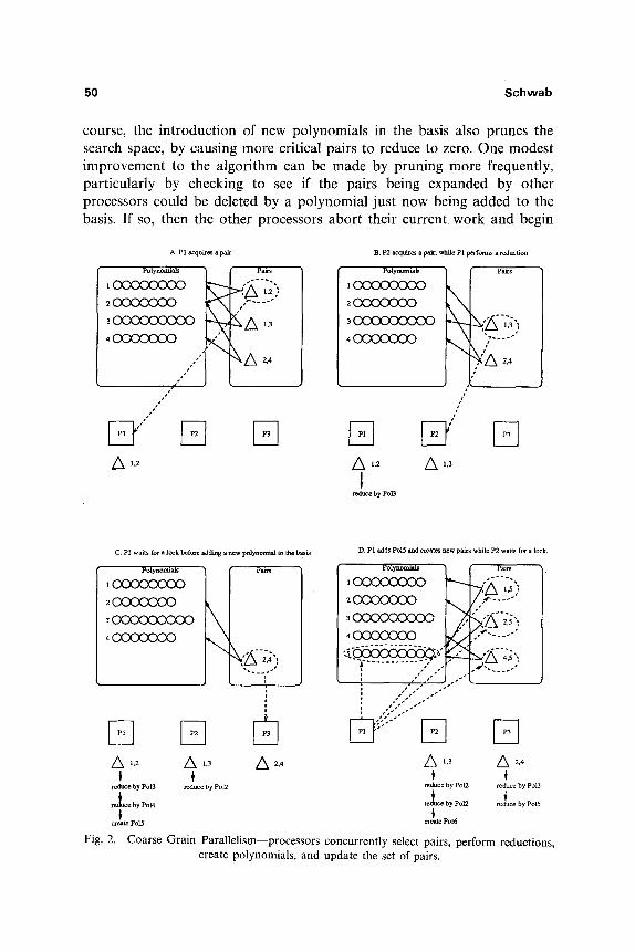
If no pairs are available when a processor acquires the lock, then it checks to see if all other processors are also waiting. If so, then the algorithm has completed, and a post-processing stage is executed. If other processors are still executing, the current processor performs a condition_wait operation until it receives a signal from another processor that new pairs are available. Figure 2 illustrates the progress of several processors executing the parallel algorithm. Note that processors can always read any polynomial, and need the lock only to add a new polynomial to the basis.

The parallelism exploited by this method is speculative parallelism, meaning that sometimes a pair will be expanded in parallel that would have been deleted in the sequential case. Speculative parallelism is the eager evaluation of a subtask in a computation before the necessity of performing this work is known. If the subtask had to be performed anyways, the algorithm benefits from increased concurrency. On the other hand, if the subtask could have been avoided, some computation time has been spent uselessly. This reduces the efficiency of the parallel algorithm because some of the work performed is useless--expanding the S-polynomial of the pair will produce, after much computation, the zero polynomial. Nevertheless, most of the pairs expanded in parallel are useful, and decrease the amount of time needed to find the Gr6bner basis. The algorithm can be viewed as a search algorithm, with the nodes to be explored being the critical pairs. A pair which reduces to the zero polynomial is a leaf node. Sometimes, expanding a critical pair produces many other pairs, which are then put on the list of work to perform, and as a side effect, we note the polynomial produced. Other pairs produce only the zero polynomial, and no new pairs to be expanded. The algorithm terminates when the search space has been completely explored, either by expanding or deleting each critical pair. Of

828/21/I-4

50 Schwab

course, the introduction of new polynomials in the basis also prunes the search space, by causing more critical pairs to reduce to zero. One modest improvement to the algorithm can be made by pruning more frequently, particularly by checking to see if the pairs being expanded by other processors could be deleted by a polynomial just now being added to the basis, If so, then the other processors abort their current work and begin

A. P1 acquires i pair

Polynomials " pairs

, o o o o o o o o

,,,,,'" ~ A 2 , 4

/ / "

A I>2

B. P2 acquires a pair, while PI Ixxforms a reduction

PolyaomiMs Pairs

' ~ ,%. ~k/A2."

s

1 ~ e by Po13

C. P1 waits for a Icck before adding a new polynomial to the basis

Polynomials

2 ~

A 1,2

1 reduce by Po13

reduce by Po14

re PoI5

PL~I*

i reduce by Pol2

Fig. 2.

D. P1 edds Po15 mad creates new pairs while i>2 waits for a lock.

Poly/loolials P~irs

, + . . . . . . �9

i . . . . . . . . . . . .." ..' ,#.."S" .." e, . t ,

i l ~ d u c e by Pol2 reduce by Pol3

cr~l~ Po16

Coarse Grain Parallelism--processors concurrently select pairs, perform reductions, create polynomials, and update the set of pairs.


work on a new pair. This reduces some of the penalty associated with the speculative parallelism.

Because this is a searching algorithm, the parallel algorithm can be expected to demonstrate super-linear speedup on some inputs because of the opportunity to expand an important pair earlier than a sequential implementation would do so. This more or less points out that some of the speedup is due not to the parallel machine we are executing on, but to the concurrent structure of the algorithm. This speedup might also occur on a uniprocessor, if the costs of context switching and memory locality overhead could be adequately minimized. Of course, an improved selection strategy for critical pairs can be expected to reduce the effects of parallel searching on the algorithm. One such improvement in selection strategy which could be incorporated into a future version of this implementation has been developed by Giovini et. al. (22)

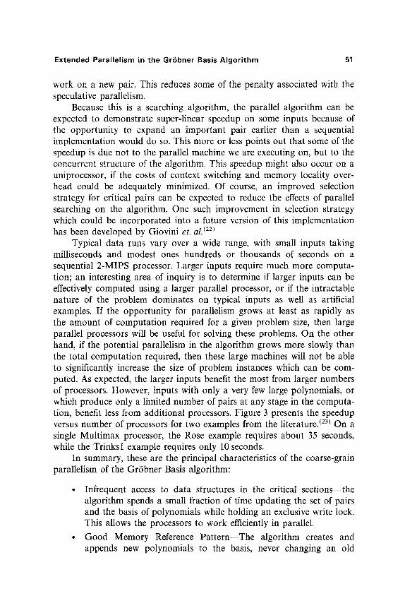
Typical data runs vary over a wide range, with small inputs taking milliseconds and modest ones hundreds or thousands of seconds on a sequential 2-MIPS processor. Larger inputs require much more computation; an interesting area of inquiry is to determine if larger inputs can be effectively computed using a larger parallel processor, or if the intractable nature of the problem dominates on typical inputs as well as artificial examples. If the opportunity for parallelism grows at least as rapidly as the amount of computation required for a given problem size, then large parallel processors will be useful for solving these problems. On the other hand, if the potential parallelism in the algorithm grows more slowly than the total computation required, then these large machines will not be able to significantly increase the size of problem instances which can be computed. As expected, the larger inputs benefit the most from larger numbers of processors. However, inputs with only a very few large polynomials, or which produce only a limited number of pairs at any stage in the computation, benefit less from additional processors. Figure 3 presents the speedup versus number of processors for two examples from the literature. (23) On a single Multimax processor, the Rose example requires about 35 seconds, while the Trinksl example requires only 10 seconds.

In summary, these are the principal characteristics of the coarse-grain parallelism of the Gr6bner Basis algorithm:

�9 Infrequent access to data structures in the critical sections--the algorithm spends a small fraction of time updating the set of pairs and the basis of polynomials while holding an exclusive write lock. This allows the processors to work efficiently in parallel.

�9 Good Memory Reference Pattern--The algorithm creates and appends new polynomials to the basis, never changing an old

52 Schwab

~ 16 / / /

0 . - . o RIB A / ' /

/ . , ~ + ,7,~

�9 / ' ~ / p

A. o / + ? " o

; , . / ; : ,,

" o s '. i o : . ' ' d ". : .'~.',, .... / ~ " / ~. . ~

i i i i i i e r

2 4 6 8 10 12 14 16

Speedups for Proble~a ROSE

~ 16

14

12

10

/ /

/

PLUS /

~ I M A X / i i - - - o +I" A - - + A /

/ /

/ , /

/ /

/

/ / /

/ / . .,t~ - ~h, . ,~t. ~ . . A

/ / .A'

�9 "~ Ja..o. ...'~'.o.-e-.o. ..o-'e~'o.. ~

i i e i = e e p

2 4 6 8 10 12 1~- 16

Speedups for Proble~n TRINKS1

Fig. 3. Grobner Basis speedup curves--voarse-grain algorithm.

polynomial. This means that on distributed memory architectures such as PLUS, the polynomials may be replicated locally on each processor. In addition, only the operations on the set of pairs require a globally shared read/write reference pattern, limiting the performance penalty of local versus global memory.

Global ordering on work--The algorithm requires that the critical pairs be processed in a particular sorted order for efficiency reasons. This prevents a structure in which each processor keeps a local work queue, and instead requires the algorithm to maintain a globally ordered work queue.

Speculative Parallelism in a Searching Algorithm--This problem may be viewed as a parallel search. As such, this parallelism is often speculative, in that the same work might not be performed by the sequential version. Because of this speculative nature, the algorithm may exhibit superlinear speed-up because some of the important critical pairs may be expanded and reduced earlier in the parallel computation than in the sequential one.

5. FINE GRAIN PARALLELISM

At the heart of the Gr6bner basis computation is the operation of reduction, in which one polynomial is used to eliminate the most significant term from an initial polynomial. Speeding up this step is critical to improving the performance of the algorithm.

The source of fine-grain parallelism in the algorithm occurs in the reduction loop. The key observation of Melenk and Neun (11) is that the


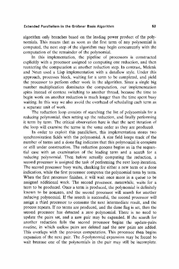
algorithm only branches based on the leading power product of the polynomials. This means that as soon as the first term of any polynomial is computed, the next step of the algorithm may begin concurrently with the computation of the remainder of the polynomial.

In this implementation, the pipeline of processors is constructed explicitly with a processor assigned to computing one reduction, and then reentering the computation at another reduction step. In contrast, Melenk and Neun used a Lisp implementation with a dataflow style. Under this approach, processes block, waiting for a term to be completed, and yield the processor to perform other work in the algorithm. Since a single big number multiplication dominates the computation, our implementation spins instead of context switching to another thread, because the time to begin work on another reduction is much longer than the time spent busy waiting. In this way we also avoid the overhead of scheduling each term as a separate unit of work.

The reduction loop consists of searching the list of polynomials for a reducing polynomial, then setting up the reduction, and finally performing it term by term. The critical observation here is that the next iteration of the loop will examine the terms in the same order as they are produced.

In order to exploit this parallelism, this implementation stores two synchronization fields with the polynomial. A size field keeps track of the number of terms and a done flag indicates that this polynomial is complete or still under construction. The reduction process begins as in the sequential case with an examination of the leading term and a search for a reducing polynomial. Then before actually computing the reduction, a second processor is assigned the task of performing the next loop iteration. The second processor busy waits, checking for either a new term or a done indication, while the first processor computes the polynomial term by term. When the first processor finishes, it will wait once more in a queue to be assigned additional work. The second processor, meanwhile, waits for a term to be produced. Once a term is produced, the polynomial is definitely known to be nonzero, and the second processor will search for another reducing polynomial. If the search is successful, the second processor will assign a third processor to consume the next intermediate result, and the process repeats. If no terms are produced, and the done flag is set, then the second processor has detected a zero polynomial. There is no need to update the pairs set, and a new pair may be expanded. If the search for another reduction fails the second processor begins the update-pairs routine, in which useless pairs are deleted and the new pairs are added. This overlaps with the previous computation. This processor then begins expansion of the next pair. The S-polynomial expansion may be forced to wait because one of the polynomials in the pair may still be incomplete.

54 Schwab

The code to compute the S-polynomials uses the same synchronization technique to consume terms as they are produced, overlapping additional computation and providing better speedup. Figure 4 illustrates the various stages in the pipelined computation.

There are several issues to point out about this pipelined reduction

( ~ ) ~ start computing first term ~ conti . . . . . . puting term by term L______A w ~ , . z - J

wait select a polylmmiaI based on the :..

first term received

~ ] wait wait

- ~ wait U ~

A B

wait

i

All Reductions Underway C

:.:

. , :

Finished ~. Update Pairs

C) term processed term

:.'i~" newly created mrm poly.o.~

Fig. 4. Pipeline Parallelism--Each processor operates on two polynomials, producing terms which are consumed by the next processor in the pipe. When no more reductions can take place, the polynomial is added to the basis.


process. (1) The busy waiting loops all spin on two cached variables. This means that the busy waiting does not saturate the bus and slow other processors down. (2) Once the reduction begins, each processor in the pipeline consumes terms at approximately the same speed as the previous processors produces them; therefore very little time is spent busy-waiting in the middle of a reduction pipeline. (3) Because the synchronization constraints flow in one direction only, no synchronization primitives are used beyond sequential consistency of reads and writes. Sequential consistency (z4'25~ is the traditional processor memory model in which reads and writes to the memory system complete in the order in which they are issued by the processor. New parallel architectures have introduced more efficient, weak ordering models. (4) There is no speculative parallelism in this part of the computation. Each reduction must be performed, and this approach simply overlaps the computation performed by the inner loop as much as possible.

Figure 5 presents the speedup versus number of processors for the Butcher example from the literature. The software mechanism was not implemented on the RP3 because of the demand for very tight coupling between processors, which was unavailable on that machine.

The principal characteristics of the fine-grain parallelism include the following:

�9 The basic reduction step can be implemented as a pipeline. This means the next operation may begin as soon as the first term of the result of the previous operation is computed.

8

/ /

/ /

/ /

/ /

/

/ /

/

/

I | ! I' i ) 2 4 6 $ lO 12

]~oocssors S p ~ d u ~ for Problem BUTCH]ER

Fig . 5. G r o b n e r B a s i s s p e e d u p c u r v e s - - f i n e - g r a i n a l g o r i t h m .

4 J"

56 Schwab

�9 The pipeline uses only a linear communication pattern in which a processor communicates with its two neighbors. This pattern should be especially well suited to a mesh architecture.

�9 The pipeline utilizes a small grain size where communication between processors takes place frequently with respect to the unit of work. This means that busy-waiting is the best method for delaying a processor in the pipeline, since other synchronization primitives are too time consuming.

�9 There is no speculative parallelism is this level of parallelism. The same work is performed here as in the sequential case. The primary loss of efficiency is due to the overhead of spinning in a tight loop while waiting for the pipeline to start processing the next reduction sequence.

6. C O M B I N I N G THE TWO LEVELS OF PARALLELISM

The two forms of parallelism described earlier combine in a com- plementary fashion. The coarse-grain method performs many reductions in parallel; the fine-grain method parallelizes the reduction chains. We experimented with a number of processor scheduling mechanisms before choosing the one used in the implementation. One version used a single work queue, another separate queues with locks, and the final version uses a fixed ordering among processors. We expect that the two forms of parallelism are independent, since performing the pair expansions in parallel, only faster, reduces the average time between pair expansion and updating the set of pairs. Because of this speedup, the fraction of time spent in the critical section updating the shared data increases. We believe that this will not become a bottleneck until hundreds of processors are used, but varying ratios of processor to synchronization speed across different architectures may make this an important consideration.

There were several steps taken in choosing the mechanism for scheduling the processes. These issues are closely coupled with the synchronization techniques used in the reduction pipeline, further complicating the problem. The first attempt to implement the algorithm used a single queue of available processors, each of which would be assigned the next reduction step anywhere in the global computatio n . All synchronization was implemented using mutex locks and C-thread conditions. The conceptual goals of this approach was clear: to provide nearly ideal load balancing as well as high-level synchronization on a tightly-coupled shared memory multiprocessor. (The Encore Multimax was the first machine on which this


technique was successfully implemented; the PLUS implementation came latter.) Unfortunately, the time between starting reduction steps was too short; the central queue became a bottleneck. At the same time, it also became clear that conditions were too heavy a synchronization primitive to use for such short duration operations as the term by term reductions in the pipeline. The first design choice was to replace the pipeline synchronization with only reads and writes. Producers signaled the completion of a term by incrementing a counter, while consumers busy-waited on the counter variable until the next term became available. The second design decision was to replace the single queue of processors with several separate queues, one for each level of coarse grain parallelism. Processors now entered these queues and busy-waited on a variable in the queue entry. When a reduction was assigned, the processor would be dequeued and would begin the reduction operation immediately, taking on the role of consumer initially, and then assigning another processor to perform the next reduction and acting as a producer of terms also. This implementation allowed some speed-up, but was still slower than expected.

Once again, the problem was the synchronization being too slow. A better design was to assign the processors a fixed order in the reduction pipeline. Each processor now consumes terms from only one processor, and its terms are in turn consumed by just one processor. The dequeue operation becomes trivial, while the enqueue operation disappears entirely. This mechanism provides the best performance, but forces some additional constraints on the implementation. In particular, a processor in the reduction pipeline can never signal the previous processor to change state or perform additional work, because there is no longer any reliable way to solve the race conditions introduced by this type of synchronization using only reads and writes. The result is that it is no longer possible to dynamically move processors between different reduction pipelines. It is difficult to measure how much performance this costs the overall algorithm, but if there is large variance in the number of reductions performed in reducing different S-Polynomials, there would be significant benefit in this type of load balancing.

Of course, on the PLUS architecture, static reduction pipelines map perfectly to processors connected by a mesh topology. Each critical pair expansion is now performed by a row of processors communicating only with two neighbors. Only updating the basis and set of pairs requires access to a globally shared memory, which improves performance of the algorithm on this type of machine.

A second type of load balancing is that of migrating processors between the coarse-grain method and the fine-grain method. Implementa- tion issues aside, it is not theoretically clear when to move processors down

58 Schwab

to the fine-grain level�9 A priori, it is impossible to determine whether one pair will be deleted by expansion of another pair. A statistical measurement of the fraction of pairs which are useful could be used as one load balancing heuristic, but a good global load balancing algorithm would have to examine the actual structure of the basis under construction and then use heuristics to decide where processors may be used most fruitfully.

In Figure 6, we present performance results for the full algorithm with both levels of parallelism�9 The Rose example is large enough to benefit from the fine-grain parallelism, while the Trinksl example is too small to speedup using this approach�9 The difference between these two problems is that the polynomials that appear in the first example tend to have 20 or more terms, while the second example has polynomials with 10 or fewer terms�9 The fine-grain parallelism only works when there are many terms to process in each polynomial. The Rose example seems to be more typical of the type of problems which arise in practice. A large multiprocessor will be able to handle problems with many more polynomials in their basis�9 Such problems are also likely to generate polynomials with proportionally more tezms and larger coefficients. Since the fine-grain parallelism operates more efficiently as the size of the polynomials increase, these larger multiprocessors will show increased speed up from this form of parallelism�9

Tables I and III compare the execution time of the algorithm on the Multimax when different ratios of processors are assigned to the coarse- grain and fine-grain parallelism�9 The execution times for the samples Rose and Butcher are presented in seconds�9 Each line in the table lists the times for an increasing number of processor groups. Each group executes an S-polynomial reduction in parallel with the other groups. In each column,

~ 30

:25

20

15

10

S

. . ~ 1 4 9 1 4 9

� 9 A PLUS , �9 � 9 �9 f f

�9 /

�9 . F ./ / .

/ . A � 9 1 4 9 , J

/ n n = i $ 10 15 2x]

S p e e d u p s f o r P r o b l e m R O S E

~ 3C

Fig. 6.

M U L ~ ] f �9 * �9 �9 PLUS j

/ /

/ J

/

IS i / J /

/ /

10i f f /

~ i n = i i 5 I0 15 2O

S l ~ e d u p s f o r P r o b l e m T R I N K S I

Gr6bner Basis speedup curves-~combined algorithm.

Extended Parallelism in the Gr6bner Basis Algorithm

Table I. Rose Example for Various Combinations of Coarse and Fine Grain Parallelism (Multimax) a

59

processors per group groups 1 2 3 4 5

1 35.3 20.2 15.3 2 11.6 8.4 6.5 3 8.6 4.8 3.8 4 5.9 4.0 2.9 5 4.9 2.7 5.3 6 4.7 2.6 7 4.6 3.1

13.3 11.9 5.7 5.6 3.4 14.43

a Execution times in seconds.

Table II. Rose Example for Various Combinations of Coarse and Fine Grain Parallelism (Plus Simulator) ~

processors per group groups 1 2 3 4 5 6

1 74.5 42.8 32.3 27.9 24.6 23.3 2 27.4 16.9 13.7 11.4 10.9 10.4 3 15.3 8.7 6.4 6.3 5.8 5.5 4 9.0 5.5 5.1 3.9 3.8 4.2 5 9.2 4.8 3.9 3.2 2.7 2.9 6 7.9 4.3 3.3 2.9 2.8 2.6

a Execution times in megacycles.

Table III, Butcher Example for Various Combinations of Coarse and Fine Grain Parallelism (Mul t imax) a

processors per group groups 1 2 3 4 5

1 307.4 185.2 138.2 110.5 96.4 2 175.3 109.7 80.4 67.8 60.2 3 132.0 82.2 62.9 57.0 137.9 4 96.7 55.1 43.8 135.3 5 89.1 54.4 66.5 6 65.9 54.9

Execution times in seconds.

3 The measured value was extremely volatile, with times falling in the range 7.0 to 21.7.

60

Table IV.

Schwab

Butcher example for Various Combinations of Coarse and Fine Grain Parallelism (Plus Simulator) a

processors per group groups 1 2 3 4 5 6

1 701.3 404.5 284.4 235.4 198.5 173.7 2 358.2 246.3 176.3 143.6 124.6 110.7 3 293.1 187.7 139.9 113.8 104.7 87.4 4 198.3 145.7 112.2 102.3 98.2 82.8 5 190.6 136.0 ! 19.3 96.6 102.0 88.2 6 296.6 132.8 103.6 93.0 79.6 92.0

Execution times in megacycles.

a different number of processors are assigned to perform fine-grain pipeline parallelism within each reduction group. For example, in the second line, the entry under the third column reports the result when six processors were used, with two separate S-polynomial reductions being performed in parallel by sets of three processors acting as a fine-grain pipeline. The table shows poor performance with 14 or 15 processors, suggesting that some type of limit in the system or algorithm has been reached. The first column indicates that relatively little improvement is observed beyond five processors using only the coarse-grain parallelism. Examination of the other columns clearly shows the benefit of assigning additional processors to perform fine-grain parallelism.

Tables II and IV presents the same comparison for execution on the Plus Simulator. Once again, we observe a gradual drop-off in the execution times as we move from left-to-right along each row. This is due to the relatively simple, uniform behavior of the fine-grain parallelism. Each column, from top-to-bottom, presents entries that exploit more coarse- grain processor groups, which exhibit faster improvements in execution times. Clearly, the Rose problem instance is well suited to the speculative parallelism used by this method. We also observe that the coarse-grain parallelism combines quite well with the fine-grain parallelism in the absence of architectural bottlenecks such as a shared bus.

7. A N A L Y S I S

One problem encountered was the difficulty of implementing the fine- grain reduction pipeline on the RP3. This form of parallelism depends on


transmitting terms from the producer to the consumer as quickly as possible. While a uniform shared-memory connecting all processors to memory via a bus provides for instant access to a term as soon as it is written, the RP3 has a relatively slow global memory accessable through a routing network. Reads and writes take place one word at a time over this network, making it difficult to pass terms efficiently between processors. Ideally, an architecture of this type should support a remote write to another processor's local memory, allowing a faster exchange of data. In this way the data would only have to traverse the network once, from producer to consumer, instead of twice, from producer to global memory, and then from global memory to the consumer. Another possibility is to provide a pipelined block transfer of data from local memory to local memory.

The RP3 memory architecture also made it difficult to store the basis locally on each processor. Even though a memory region could be replicated to a set of processors, no provision was made for broadcasting new data to the replicated memory. In order to achieve this functionality, each processor would have to check the global data structure and manually copy the new data to its local memory. While this is consistent with the philosophy of not providing cache coherency on the machine, it makes the implementation slower, and more complex, than it otherwise would be.

Finally, no provision was made to provide interprocessor interrupts directly to the user process. This feature, which allows one processor to efficiently signal another, could have been used to provide better synchronization, especially a busy-waiting implementation of the mutual exclusion algorithm. Note that without this feature, busy-waiting requires continuous references to the global memory, causing increased contention for this critical resource, and thereby slowing down other processors doing useful work.

In contrast, Plus provides a much more closely coupled memory system through replicated memory. Writing to a local memory location which is replicated transparently sends a message carrying the new data to other processors. This allows for efficient fine-grain performance, which is critical to utilizing larger numbers of processors efficiently. In addition, a mesh topology is well suited to this problem because the fine-grain form of parallelism may be arranged as a line of neighbor-to-neighbor communication. It is necessary to replicate the basis to all processors, but since updating the basis occurs infrequently, the impact on overall performance is relatively limited. In a large system with 256 or more processors, the interconnection network might become overloaded because some processor would almost always be writing and replicating a new basis polynomial. One technique to limit this effect would be to split the processors into even

62 Schwab

and odd groups-each processor would store only half the basis, decreas- ing network load. Each polynomial would, on average, pass through one additional processor in the reduction pipeline, introducing very little additional cost. This technique could be generalized to any number of processor splitting sets, with processors selecting polynomials either deterministically or randomly.

8, RELATED W O R K

Buchberger has described a distributed-memory algorithm to compute Gr6bner bases on the L-machine, a parallel machine designed to support parallel symbolic computation. (9~ The main idea from this work was to dedicate one processor to manage the set of critical pairs, and use the rest to distribute and reduce the S-polynomials. The algorithm was described for both a tree of processors and a ring topology. In addition to distributing multiple critical pairs to the worker processors for reduction, the managing processor will also halt a reduction in progress if it becomes useless due to the addition of a new polynomial to the basis. By using this policy of eagerly killing off useless computation, the penalty for speculative computation is expected to be reduced. A more complete analysis of the effect of including this feature in a parallel implementation is needed to determine if it actuality improves execution time. No performance numbers have been reported for this work.

Watt explored the use of remote-procedure call as a primitive for parallel computer algebra on a network of machines. (8~ This lead to an algorithm which performed a number of pair reductions in parallel, waiting for all the reductions to complete before a parallel phase in which all polynomials were interreduced with respect to the rest of the basis. Ponder (~~ demonstrated that this algorithm fails when two polynomials with the same leading term eliminate this term completely from the basis during the parallel interreduction. Also, due to the data structures used, the same S-polynomials could be expanded and reduced to 0 several times during execution. Ponder modified this approach to parallelize only the critica! pair reduction or the basis interreduction, executing the other phase sequentially. This resulted in a correct implementation, but very little parallel speedup. In addition, the theoretical constraints used to eliminate many critical pairs with only minimal computation were not included in this implementation. Two other parallel approaches where also studied by Ponder_ The first involved finding GrSbner bases for subsets of the input and then merging the results together in a divide-and-conquer paradigm. Unfortunately, the merge step was prohibitively expensive. The second approach was to speculate by running multiple independent computations,


each using a different ordering. Since the time to compute the result may depend on the selected ordering, this could result in a fair speedup, although this was not demonstrated. A better technique may be to start with a partial term ordering, and select a specific refinement of the ordering as needed by the computation. By using speculative parallelism to evaluate several refinement orderings in parallel, an efficient algorithm could be developed.

Siegl (26) and Senechaud (13) have implemented distributed versions of the algorithm. Siegl selected Strand88 as an implementation language, and demonstrated an efficent algorithm on a linear topology. S-polynomials where reduced in parallel as they moved from processor to processor until reaching the end of the list of polynomials, stored one to a processor. The next processor then adds itself to the list, and stores this new polynomial. At the same time, new polynomials move up the line of processors, reducing the old polynomial stored there. In this way, critical pair expansion and interreduction are performed concurrently. Reported speedups ranged from 1.5 to 8.3, which were quite good considering that the structure of the algorithm allowed maximum theoretical speedup of only one-half the number of polynomials in the basis, and the examples where small. Unfortunately, the actual running times were quite slow, because of the inefficiency of Strand88 for implementing the basic mathematic and reduction operations. Senechaud restricts the algorithm to Boolean polynomials, where the only coefficients and exponents are 0 and 1. A limited degree of speedup was reported, perhaps because the criteria for eliminating useless pairs was not implemented.

Gradually, the work in this area is evolving from the proposal of parallel algorithms based upon expected performance and bottlenecks to the refinement of parallel implementations based upon actual execution behavior. Als0, as the architectures and language tools available for parallel computation improve, more sophisticated implementations that match the requirements of the Gr6bner basis computation to the primitives available are being developed.

9. C O N C L U S I O N

The computation of Gr6bner bases can be carried out in parallel. Taking advantage of better algorithms, larger machines and scalable architectures will allow much larger problems to be solved, as long as they do not exhibit the intractable behavior of some of the artificial examples. There are two different parallel techniques combined in this implementation, demonstrating that better overall performance can be achieved in this way,

64 Schwab

as opposed to relying on only one method of parallelism. The cost of this is added complexity in the algorithm, especially in the areas of load balancing and scheduling of processors. In addition, this implementation appears very suitable for one type of nonuniform access shared memory machine. Future work should address how much and what type of resources can be favorable exploited by this algorithm as well as other symbolic computations. In addition, experimental evidence and theoretical insight need to be combined to provide good heuristics for migrating processors between the two methods of parallelism, and better software tools and implementation techniques are needed to actually make such an implementation of the algorithm perform efficiently on larger machines.

The main contributions of this work include:

�9 Demonstrating that two distinct types of parallelism may be combined in this algorithm to produce a more efficient implementation.

�9 Examining the methods and issues involved in scheduling processors between the two parallel methods.

�9 Utilizing more processors by implementing an algorithm that can effectively run on an architecture other than a bus-based shared memory multiprocessor, which is limited in size.

There are several other directions in which to pursue the Gr6bner basis algorithm. One is the implementation on a massively parallel architecture, such as the Connection Machine. Both implementation issues, such as the methods of coercing a decidedly MIMD algorithm with speculative parallelism into a deterministic SIMD form, as well as theoretical issues, such as the complexity of the algorithm over stronger computation models with unit time primitives for integer multiplication and reduction need to be considered. Another promising area to investigate is the technique of using multiple orderings in the same computation, or of con- structing or modifying the ordering as the computation unfolds, to increase performance. A third issue of concern is the behavior of the algorithm on completely distributed machines, including large hypercubes and general network-connected distributed systems. Finally, a survey of the practical uses of the algorithm, and case studies of real world problems solvable by utilizing Gr6bner bases are necessary to determine where to concentrate future effort in improving implementations of the algorithm. The Proteus version of the implementation is available via ftp from ftp.cs.cmu.edu, in the file/afs/cs/user/schwab/ftp/grobner.tar.Z. This version of the code runs on DecStation5000 and DecStation3100 workstations.


ACKNOWLEDGMENTS

Many thanks to Jean-Phillipe Vidal for implementing the first parallel version of the algorithm on the Encore Multimax, and for his encourage- ment in studying this problem. Also, I want to thank Edmund Clarke for his support in pursuing this research, as well as help in presenting it to many visitors at Carnegie Mellon and the research community at large. Finally, thanks go to David Long, Spiro Michaylov, and Brian Bershad for their help in revising and editing earlier drafts of this paper.

REFERENCES

1. Robin Hartshorne, Algebraic Geometry: Graduate Texts in Mathematics, Volume 52, Springer-Verlag, New York (1977).

2. Bruno Buchberger, An Algorithm for Finding a Basis for the Residue Class Ring of a Zero-Dimensional Polynomial Ideal (German). Phi) Thesis, University of Innsbruck, (1965).

3. Bruno Buchberger, Gr6bner bases: An Algorithmic Method in Polynomial Ideal Theory, (ed.), N.K. Bose, Recent Trends In Multidimensional Systems Theory, D. Reidel Publishing Company, pp. 184-232, (1985).

4. B. Misra and C. Yap, Notes on Gr6bner Bases, Information Seiences, 48:219-252 (August 1989).

5. Jean Philippe Vidal, The Computation of Gr6bner Bases on a Shared Memory Multi- processor, Technical Report CMU-CS-90-163, Computer Science Department, Carnegie Mellon University (August 1990).

6. Riidiger Gebauer and Michael M611er, On an Installation of Buchberger's Algorithm, Journal of Symbolic Computation, 6(2, 3):275-286 (1988).

7. Ernst W. Mayr and Albert Meyer, The Complexity of the Word Problems for Com- mutative Semiigroups and Polynomial Ideals, Advances in Mathematics, 46:305-329 (1982).

8. Stephen M. Watt, Bounded Parallelism in Computer Algebra, PhD Thesis, University of Waterloo (May 1986).

9. Bruno Buchberger, The Parallelization of Critical Pair/Completion Procedures on the L-Machine, Proe. of the Japanese Symp. on Functional Programming, pp. 54-61 (February 1987).

10. Carl Glen Ponder, Evaluation of 'Performance Enhancements' in Algebraic Manipulation Systems. Ph.D thesis, University of California, Berkeley (August 1988).

11. Herbert Melenk and Winfried Noun, Parallel Polynomial Operations in the Large Buchberger Algorithm, Computer Algebra and Parallelism, Workshop at the TIM3 Laboratory, U~iversity of Grenoble, France. Academic Press, London {June 1988).

12. Kurt Siegl, A Parallel Version of Buchberger's Algorithm in STRAND88, Technical Report RISC-Linz 90-17.0, Johannes Kepler University, Linz, Austria (1990).

13. Pascale Senechaud, Implementation of a Parallel Algorithm to Compute a Gr6hner Basis on Boolean Polynomials, Computer Algebra and Parallelism, Workshop at the TIM3 Laboratory, University of Grenoble, France, Academic Press, London, pp. 159-166 (June 1988).

14. Encore Computer Corporation, Multimax Technical Summary (1986). 15. IBM. Research Parallel Processor Prototype Principle of Operations.

828/21/145

66 Schwab

16. R. Bisiani and M. Ravishankar, PLUS: A Distributed Shared-Memory System, Proc. of the 17th Ann. Symp. on Comp. Archit. IEEE Computer Society Press (June 1990).

17. Eric A. Brewer, Chrysanthos N. Dellarocas, Adrian Colbrook, and William E. Weihl, Proteus: A High-Performance Parallel Architecture Simulator, Technical Report MIT/LCS/TR-516, MIT, Laboratory of Computer Science (1991).

18. E. C . Cooper, C-Threads, Technical Report CMU-CS-88-154, Carnegie Mellon University, Pittsburgh, Pennsylvannia (June 1988).

19. R. V. Baron, R. F. Rashid, E. Siegel, A. Tevanian, and M. W. Young, MACH-I:A Multi- processor Oriented Operating System and Environment, New Computing Environments: Parallel, Vector and Symbolic. S lAM (1986).

20. David L. Detlefs, Concurrent, Atomic Garbage Collection. PhD Thesis, Carnegie Mellon University (October 1990).

21. Bruno Buchberger, A Criterion for Detecting Unnecessary Reductions in the Construction of Gr6bner Bases, Proc. of EUROSAM 79, Lectures Notes in Computer Science, 72:3-21 (1979).

22. A. Giovini, T. Mora, G. Niesi, L. Robbiano, and C. Traverso. "One Sugar Cube, Please" or Selection Strategies in the Buchberger Algorithm, Proc. of the lnt'l. Syrup. on Symbolic and Algebraic Computation, ACM, New York, pp. 49 54. (July 1991).

23. W. Boege, R. Gebauer, and H. Kredel, Some Examples for Solving Systems of Algebraic Equations by Calculating Groebner Bases, Journal of Symbolic Computation, 1:83-98 (1986).

24. 24. Sarita V. Adve and Mark D. Hill, Weak Ordering--A New Definition. The 17th Ann. Int'L Symp. on Comp. Archit. (June 1990).

25. L. Lamport, How to Make a Multiprocessor Computer That Correctly Executes Multiprocess Programs. 1EEE Trans. on Computers, C-28:690-691 (September 1979).

26. Kurt Siegl, Gr6bner Bases Computation in STRAND: A Case Study for Concurrent Symbolic Computation in Logic Programming Languages. PhD Thesis, RISC-LINZ, Johannes Kepler University (November 1990).

Date post:	21-Apr-2018
Category:	Documents
Upload:	ngomien
View:	215 times
Download:	0 times

Extended parallelism in the Gröbner basis...

Documents