EXTENDING THE PETREL MODEL BUILDER FOR EDUCATIONAL AND
RESEARCH PURPOSES
A Thesis
by
OBIAJULU CHUKWUDI NWOSA
Submitted to the Office of Graduate Studies of
Texas A&M University
in partial fulfillment of the requirements for the degree of
MASTER OF SCIENCE
Approved by:
Chair of Committee, Eduardo Gildin
Committee Members, Mike King
Yuefeng Sun
Head of Department, Dan Hill
May 2013
Major Subject: Petroleum Engineering
Copyright 2013 Obiajulu Chukwudi Nwosa
ii
ABSTRACT
Reservoir Simulation is a very powerful tool used in the Oil and Gas industry to
perform and provide various functions including but not limited to predicting reservoir
performance, conduct sensitivity analysis to quantify uncertainty, production
optimization and overall reservoir management. Compared to explored reservoirs in the
past, current day reservoirs are more complex in extent and structure. As a result,
reservoir simulators and algorithms used to represent dynamic systems of flow in porous
media have invariably got just as complex. In order to provide the best solutions for
analyzing reservoir performance, there is a need to continuously develop reservoir
simulators and reservoir simulation algorithms that best represent the performance of the
reservoir without compromising efficiency and accuracy.
There exists several commercial reservoir simulation packages in the market that
have been proven to be extremely resourceful with functionality that covers a wide range
of interests in reservoir simulation yet there is the constant need to provide better and
more efficient methods and algorithms to study and manage our reservoirs. This thesis
aims at bridging the gap in the framework for developing these algorithms. To this end,
this project has both an educational and research component. Educational because it
leads to a strong understanding of the topic of reservoir simulation for students which
can be daunting especially for those who require a more direct experience to fully
comprehend the subject matter. It is research focused because it will serve as the
foundation for developing a framework for integrating custom built external simulators
iii
and algorithms with the workflow of the model builder of our reservoir simulation
package of choice i.e. Petrel with the Ocean programming environment in a seamless
manner for simulating large scale multi-physics problems of flow in highly
heterogeneous flow of porous media.
Of particular interest are the areas of model order reduction and production
optimization. In-house algorithms are being developed for these areas of interest and
with the completion of this project. We hope to have developed a framework whereby
we can take our algorithms specifically developed for areas of interest and add them to
the workflow of the Petrel Model Builder.
Currently, we have taken one of our in-house simulators i.e. a two dimensional,
oil-water five-spot water flood pattern as a starting point and have been able to integrate
it successfully into the “Define Simulation Case” process of Petrel as an additional
choice for simulation by an end user. In the future, we will expand this simulator with
updates to improve its performance, efficiency and extend its capabilities to incorporate
areas of research interest.
v
ACKNOWLEDGEMENTS
I want to take this opportunity to thank everyone that was instrumental directly or
indirectly in helping me accomplish my research objectives. Of note is my Committee
Chair, Dr. Eduardo Gildin and other committee members, Dr. Mike King and Dr.
Yuefeng Sun.
I would also like to extend my gratitude to Schlumberger for giving me access to
the relevant software and tools to complete this project on schedule and to the Society of
Petroleum Engineering, Dallas Section for the grant awarded to me.
Finally, I would like to thank my family for all their encouragement and support.
vi
TABLE OF CONTENTS
Page
ABSTRACT .......................................................................................................................ii
DEDICATION .................................................................................................................. iv
ACKNOWLEDGEMENTS ............................................................................................... v
TABLE OF CONTENTS .................................................................................................. vi
LIST OF FIGURES ........................................................................................................ viii
LIST OF TABLES ...........................................................................................................xii
CHAPTER I INTRODUCTION AND LITERATURE REVIEW ............................... 1
Introduction .................................................................................................................. 1
Motivation .................................................................................................................... 5
Literature Review ......................................................................................................... 6
Scope of Study ............................................................................................................. 9
CHAPTER II MODEL CONSTRUCTION ................................................................. 12
Partial Differential Flow Equations ............................................................................ 13
Discretization of Partial Differential Equations ......................................................... 17
Structure of Matrices ................................................................................................. 27
CHAPTER III MODEL IMPLEMENTATION IN PETREL ....................................... 31
Introduction ............................................................................................................... 31
Model Inputs ............................................................................................................. 33
Model Construction ................................................................................................... 37
Results ....................................................................................................................... 60
vii
CHAPTER IV OCEAN IN PETREL AND CUSTOM SIMULATOR ........................ 67
Ocean in Petrel .......................................................................................................... 67
How to Make a Plug-in ............................................................................................. 70
Custom Simulator ...................................................................................................... 78
Results ....................................................................................................................... 89
CHAPTER V COMPARISON OF RESULTS AND CONCLUSIONS ..................... 97
Root Mean Square Error Analysis ............................................................................ 97
Pressure and Time-Step Analysis ............................................................................ 106
Recommendation ..................................................................................................... 115
Future Work and Conclusion .................................................................................. 115
REFERENCES ............................................................................................................... 118
viii
LIST OF FIGURES
Page
Figure 1: Process Flow for Custom Simulator Plug-in .................................................... 11
Figure 2: 5-point Stencil ................................................................................................... 13
Figure 3: Picture of Implemented Reservoir Model ......................................................... 32
Figure 4: The Process Flow Chart for our Simulator Code .............................................. 36
Figure 5: New Project Settings ......................................................................................... 38
Figure 6: Selection of Make Simple Grid ......................................................................... 39
Figure 7: Make Simple Grid (Input Data Tab) ................................................................. 40
Figure 8: Make a Simple Grid (Geometry Tab) ............................................................... 41
Figure 9: Conversion to Surface ....................................................................................... 42
Figure 10: Surfaces for 11x11(Input Pane) ...................................................................... 42
Figure 11: Make Horizon in Processes Tab ..................................................................... 43
Figure 12: Make Horizon with 11x11 .............................................................................. 44
Figure 13: Layering Process ............................................................................................. 44
Figure 14: Property Calculator ......................................................................................... 45
Figure 15: Porosity and Permeability Calculation ........................................................... 46
Figure 16: Porosity Property in a 3D Window ................................................................. 47
Figure 17: Make Fluid Model Window General Tab ....................................................... 49
Figure 18: Make Fluid Model (Initial Condition Tab) ..................................................... 50
Figure 19: Oil Formation Volume Factor and Oil Viscosity for Dead Oil ...................... 51
Figure 20: Make Rock Physics Functions (Saturation Tab) ............................................ 52
Figure 21: Make Rock Physics Functions (Compaction Tab) ......................................... 53
ix
Figure 22: Make Development Strategy .......................................................................... 54
Figure 23: Make Development Strategy (Adding Rules) ................................................. 55
Figure 24: Define Simulation Case (Grid) ....................................................................... 56
Figure 25: Define Simulation Case (Drainage Relative Permeability) ............................ 57
Figure 26: Define Simulation Case (Rock Compaction) ................................................. 58
Figure 27: Define Simulation Case (Initial Condition) .................................................... 59
Figure 28: Define Simulation Case (Development Strategy) ........................................... 60
Figure 29: Oil Production Rates for the 4 Producers with Eclipse 100 ........................... 61
Figure 30: Water Production Rates for all 4 Producers with Eclipse 100 ........................ 62
Figure 31: Water Saturation Map at 100 Days with Eclipse 100 ..................................... 63
Figure 32: Water Saturation Map at 200 Days with Eclipse 100 ..................................... 64
Figure 33: Pressure Map at 100 Days with Eclipse 100 .................................................. 64
Figure 34: Pressure Map at 200 Days with Eclipse 100 .................................................. 65
Figure 35: Petrel User Interface (Adapted from Ocean Software Development Kit
Fundamental Training Volume 1) .................................................................. 69
Figure 36: Ocean Templates in Visual Studio ................................................................. 70
Figure 37: Choosing Ocean Template .............................................................................. 71
Figure 38: Ocean Plug-in Create - Step 1 ........................................................................ 72
Figure 39: Ocean Plug-in Create - Step 3 ........................................................................ 73
Figure 40: Ocean Plug-in Create - Step 4 ........................................................................ 73
Figure 41: Ocean Plug-in Create - Step 5 ........................................................................ 74
Figure 42: Instance of Plug-in .......................................................................................... 75
Figure 43: Instance of Module ........................................................................................ 75
Figure 44: ExecuteSimple Method ................................................................................... 76
x
Figure 45: OceanModuleWorkstep .................................................................................. 77
Figure 46: Reservoir Simulation in Petrel (Slide Courtesy of Schlumberger) ................. 79
Figure 47: Process for Developing a Custom Simulator .................................................. 80
Figure 48: Student Simulator in Define Simulation Case ................................................ 81
Figure 49: Student Simulator and Custom Tab ................................................................ 82
Figure 50: Format of the Code to Generate Dll File ........................................................ 83
Figure 51: Format to Pass Inputs From Petrel to Custom Simulator ............................... 85
Figure 52: RunSimulationMethod Code .......................................................................... 86
Figure 53: Oil Production Rate with Custom Simulator .................................................. 89
Figure 54: Water Production Rate with Custom Simulator ............................................. 90
Figure 55: Water Saturation at 100 Days with Custom Simulator ................................... 90
Figure 56: Water Saturation at 200 Days with Custom Simulator ................................... 91
Figure 57: Pressure Map at 100 Days with Custom Simulator ........................................ 91
Figure 58: Pressure Map at 200 Days with Custom Simulator ........................................ 92
Figure 59: Oil Production Rates - Custom Simulator ...................................................... 93
Figure 60: Water Production Rates - Custom Simulator .................................................. 94
Figure 61: Water Saturation at 100 Days - Custom Simulator......................................... 94
Figure 62: Water Saturation at 200 Days - Custom Simulator........................................ 95
Figure 63: Pressure at 100 Days - Custom Simulator ..................................................... 95
Figure 64: Pressure at 200 Days - Custom Simulator ...................................................... 96
Figure 65: Oil Production Rate of P1 with both Simulators (Homogeneous Case) ......... 98
Figure 66: Water Production Rate of P1 with both Simulators (Homogeneous Case) .... 98
Figure 67: Oil Production Rate of P2 with both Simulators (Homogeneous Case) ........ 99
Figure 68: Water Production Rate of P2 with both Simulators (Homogeneous Case) .... 99
xi
Figure 69: Oil Production Rate of P1 with both Simulators (Heterogenous Case) ........ 101
Figure 70: Water Production Rate oF P1 with both Simulators (Heterogenous Case) .. 102
Figure 71: Oil Production Rate of P2 with both Simulators (Heterogenous Case) ........ 102
Figure 72: Water Production Rate of P1 with both Simulators (Heterogenous Case) .. 103
Figure 73: Oil Production Rate of P3 with both Simulators (Heterogenous Case) ........ 103
Figure 74: Water Production Rate of P3 with both Simulators (Heterogenous Case) ... 104
Figure 75: Oil Production Rate of P4 with both Simulators (Heterogenous Case) ........ 104
Figure 76: Water Production Rate of P4 with both Simulators (Heterogenous Case) ... 105
Figure 77: Pressures from Eclipse 100 and Custom Simulator on February 15th ......... 107
Figure 78: Pressures from Eclipse 100 and Custom Simulator on April 15th ............... 108
Figure 79: Pressures from Eclipse 100 and Custom Simulator on June 15th ................ 108
Figure 80: Pressures from Eclipse 100 and Custom Simulator on August 15th ............ 109
Figure 81: Pressures from Eclipse 100 and Custom Simulator on October 1st ............. 109
Figure 82: Oil Production Rate of P2 with Custom Simulator (0.001Timestep) ........... 112
Figure 83: Water Production Rate of P2 with Custom Simulator (0.001Timestep) ...... 112
Figure 84: Oil Production Rate of P3 with Custom Simulator (0.001Timestep) ........... 113
Figure 85: Water Production Rate of P3 with Custom Simulator (0.001Timestep) ...... 113
xii
LIST OF TABLES
Page
Table 1: Inputs of Simulator ............................................................................................. 33
Table 2: Water and Oil Relative Permeability as a Function of Water Saturation .......... 34
Table 3: Oil Formation Volume Factor and Oil Viscosity as a Function of Pressure ...... 34
Table 4: Rms Error of Production Rate for all Producers (Homogenous Case) ............ 100
Table 5: Rms Error of Production Rate for all Producers (Heterogenous Case) ........... 105
Table 6: Pressure Rms Analysis between both Simulators (Heterogenous Case) ......... 110
Table 7: Rms Production Rate at 0.001 and 0.2 Timesteps for P2 and P3 .................... 114
1
CHAPTER I
INTRODUCTION AND LITERATURE REVIEW
Introduction
A Reservoir Simulator is a computer generated model that aims to represent the
full geological extent and structure of a reservoir. The reservoir simulator gives the
reservoir engineer the ability to study and analyze the performance of the reservoir under
various operating conditions in order to adopt an efficient and maximum profit-driven
development strategy for producing hydrocarbons from the reservoir.
As part of this effort to develop an appropriate management strategy, the
reservoir engineer works with an interdisciplinary team made up of geologists,
geophysicists, production engineers, drilling engineers and other functions to develop a
reservoir management plan. Developing a reservoir management plan is a long process
that first begins with adopting a strategy. According to Hoang et al. (1992), “recognizing
the specific need and setting a realistic and achievable purpose are the first steps in
reservoir management.” During this stage, the nature of the reservoir from its
characterization i.e. geology, rock and fluid properties, fluid flow, recovery mechanisms
to be implemented, drilling and well completion and past production performance are
established.
Following reservoir characterization, is a study of the “total environment” to
better understand the co-operate goals, culture, political stability, economic climate,
social issues including safety and environmental regulations. The next stage is
developing operational strategies for depleting the reservoir to recover hydrocarbons.
2
Data acquisition and analysis is conducted to further understand the nature of the
reservoir and with the information gathered, we are able to feed inputs to geological
models and numerical simulators to calibrate against historic production data and
conduct prediction runs for future reservoir performance under various operating
conditions. There are many stages in the reservoir management process including but not
limited to strategy implementation, evaluation and monitoring but in all cases, accurate
reservoir simulation is of central importance due to its connection to all phases of the
management plan. In this project, we focus on the reservoir simulation stage of reservoir
management.
To conduct reservoir performance prediction, simulation studies and analysis,
many commercial reservoir simulation packages are available in the market. Reservoir
simulation technology has gone through lots of changes from times of simplified models
to give estimates of reservoir performance to reservoir simulators that are capable of
capturing in great detail the structure and dynamic nature of a reservoir and provide very
accurate results. Reservoir simulators are developed based on a set of partial differential
equations that govern the flow of hydrocarbons in highly heterogeneous porous media.
Current commercial reservoir simulators have the ability to simulate single phase and
multiphase flow behavior in porous media and represent complex geology with complex
geometry systems in an increasing order of billions of grid blocks in size. Although very
efficient numerical solution techniques have been implemented in these industrial
strength software packages, the large scale nature of many reservoir models still pose
difficulty in getting results in a timely manner. This difficulty is evident especially when
3
one couples optimization algorithms in which several runs of forward modeling are
required to complete the specific task. It is with this realization of increased system
complexity that many model reduction algorithms have been developed in recent years
Antoulas (2005), Gildin et al. (2006), Gildin and Lopez (2011). In this case, reduced
order models can represent such large and complex reservoirs with both lower
complexity and less computationally demanding models that will capture subsurface
behavior and physical attributes without compromising efficiency and accuracy.
As mentioned by Hoang et al. (1992), during the reservoir characterization stage
of reservoir management, very important information concerning the nature of the
fluid(s) flowing, the nature of the rock and other important information are established.
Reservoir simulators are designed with the capability to model the variation in structure
of porous media to give a good representation of the reservoir in order to calibrate the
model against past production and use as a base to conduct predictions of reservoir
performance. Among these simulation packages, one can single out Petrel (Petrel
Reservoir Engineering), the Pre and Post Processor of Eclipse (ECLIPSE Reservoir
Engineering), which are both owned by Schlumberger. Petrel gives a user access to three
types of simulators namely a black oil simulator i.e. Eclipse 100, a compositional
simulator i.e. Eclipse 300 and FrontSim, the streamline simulator. As part of building
simulation models, the user of Petrel has the ability to create a “simulation case” using
processes in the process pane that span every domain of Petrel from Reservoir
Engineering, Production Engineering, Geophysics and Geology to develop a simulation
case.
4
The Model builder of Petrel has a lot of functionality to prepare simulation cases
for reservoir simulation but as implied earlier, reservoir simulation is continually
growing and so functionality that captures these developments in reservoir simulation
have to be incorporated into the workflow process of developing models in model
builders. New efficient algorithms to enhance performance and provide more accurate
solutions are developed frequently based on the research in academia, industry and other
third parties. A major part of this project is to extend the functionality of Petrel by using
the Schlumberger accompanying application program interface, Ocean-in-Petrel which
enables a software developer to program new processes and efficient algorithms that
provide unique solutions and add them to the Petrel workflow for creating models and
cases for reservoir simulation.
The objective of this project is to develop a framework for incorporating in-
house developed algorithms that provide our unique solutions into the workflow of
Petrel in the form of custom external reservoir simulators among the choices of
simulators for simulation of reservoir simulation cases. Currently, under the supervision
of my advisor and a Schlumberger Software Development team, I have achieved this
goal by using my two-phase, two-dimensional oil-water 5-Spot water flood pattern
simulator as a basis and implemented the equivalent external custom simulator. The
outputs of the custom simulator are visualization of pressures, water and oil saturation
maps at any given time along with the production rates of oil and water.
As the product of this project will be used in a classroom environment, it is our
belief that this project will have immense educational value for students as it will
5
explore various aspects of reservoir simulation and show how models under various
operating conditions perform by accepting input data and making a development strategy
and finally defining a simulation case to be simulated in a timely manner. We believe
that this project will serve as the foundation for a series of external custom simulators
(plug-ins) in the general area of closed-loop reservoir management, model reduction and
production optimization.
Motivation
In many scientific development and practical applications, one is faced with the
task of simulating and controlling complex dynamic systems. In reservoir simulation, the
key challenges are to represent oil and gas reservoirs both as realistically and accurately
as possible in order to provide scenarios of prediction under various operating conditions
to select an optimal development strategy for reservoir management.
A major challenge of reservoir simulation is the accurate geological
representation of large scale models by numerical simulators. These simulators are
mathematical models derived from first principle, conservation laws and profound
knowledge of material physics as its foundation and discretized sets of partial
differential equations. In order to represent these large scale reservoirs, highly accurate
and detailed description induced dynamic systems of large dimensions in the state space
as millions of grid blocks are often necessary in the discretization process. Direct
numerical simulation of the associated large scale models leads to unmanageable large
demands in computational effort often requiring massive parallel computation, complex
hardware and trade-off between accuracy and complexity. To avoid the challenges of
6
direct simulation, proposed methods such as Upscaling as mentioned by Christie (1996),
Chen et al. (2005) which is a tool used to develop geo-statistical reservoir descriptions
has become increasingly popular to represent fine scale descriptions of reservoir
porosity, permeability and other flow functions with coarser scale models more suitable
for simulation grids.
As mentioned, model order reduction can be used to obtain fast simulation
models Christie (1996), Chen et al. (2005). The Framework created in this project can be
easily extended to incorporate the reduced order model when available into the Petrel
software package. In this case, when these algorithms are fully developed, plug-ins that
contains reduced models will be added to the workflow of the Petrel Model Builder and
be made available possibly for commercial use.
Literature Review
Petrel is the pre and post processor of Eclipse a reservoir simulation interface that
is well known in the Oil and Gas Industry. With Petrel, a user is able to develop
reservoir simulation cases that aid in studying and analyzing the performance of
reservoirs under various operating conditions to facilitate final decision making for
reservoir management. I began my literature review by bearing in mind the sole
objective of this project which is to develop a framework and foundation for extending
the reservoir model builder in Petrel for reservoir simulation of defined simulation cases.
Suffice to say, this project is more software development centric than it is about making
considerable improvement in a particular area of research. The end product will
document our way of extending the functionality of Petrel by implementing an external
7
custom simulator with an in-house developed two-phase, two-dimensional oil-water 5-
spot water flood pattern.
For all intent and purposes, this is a literature review but in actual sense, this is
the process of how I came to understand and learn how to extend the functionality of
Petrel. It began by undergoing the training conducted by Schlumberger on Ocean-In-
Petrel Software Development Kit, which is the application program interface through
which a software developer can work in any domain of reservoir modeling such as
Production Engineering, Reservoir Engineering, Geology etc. and apply their creativity
and develop extensions or plug-ins to implement algorithms to add to the workflow of
Petrel for model building.
In the Ocean store “www.ocean.slb.com”, which is the one stop shop to purchase
plug-ins that have been developed by software developers, you will find custom
solutions in different areas of interest spanning every domain of reservoir model
building and analysis. This brings me back to the motivation for this project. To have a
good idea of where we are going, we need to have an equally good idea of the past, what
has been achieved and the areas where attention is most needed. Reservoir simulation
tools come in various forms from simple mathematical models to complicated computer
generated simulators for predicting reservoir behavior (Blackwell and Richardson 1971).
In this project, we are more interested in computer generated simulators. After the
inception of computer generated reservoir simulators, the main issues encountered
involved but weren’t limited to simulation speed, computational demand, accuracy and
general efficiency (Watts et al. 1997).
8
As computing speed and power increased, so did the ability to model subsurface
geological structures with large numbers of grid blocks, complex geometry requiring
complex gridding schemes. The capability of reservoir simulators has gone from being
able to handle single-phase, one-dimensional models to multiphase three-dimensional
models. According to Watts et al. (1997), “many of the advances in computational
methods made the technical transition possible.” Some of these advances include
Aronofsky and Jenkins radial gas model, Alternating-direction implicit procedure,
IMPES computational method, Upstream weighting, Implicit method, Geostatistics,
Upscaling, Voronoi griding etc.
To the benefit of end users, all the afore-mentioned computational advances are
included in most reservoir simulating packages today to simulate multiphase fluid
models of varying dimensions, realistic geometries, well conning, compositional
simulation, simulation of miscible fluid models, fractured reservoirs, integration with
non-reservoir computations etc.
As computing power increased, simulation of reservoirs that were once thought
impossible became more feasible. Among such reservoirs are those that require large
number of grid blocks of the order of billions of grid blocks with complex geometry that
impose heavy computational demands on our simulators. In the industry, to solve these
large scale problems, solutions such as Upscaling have been adopted where a fine grid
with properties of porosity, permeability and flow functions are represented with a
system of smaller grids that maintains the structure and implicit physical nature of the
9
reservoir with the goal of reducing computational cost, demand and provide solutions
that doesn’t compromise accuracy and efficiency.
Another proposed solution is model order reduction which is a counterpart of
upscaling which also aims to represent the finer grid model with a coarser grid model
with the main distinguishing factor being the algorithms implemented to reduce to a
system of smaller states. Model order reduction and production optimization is a key
area of interest and like other areas in reservoir simulation that have undergone
breakthroughs over the years, our research team is focusing on making strides in these
areas. It is the intention of this thesis, that with the framework for extending the
functionality of Petrel established, already developed plug-ins such as the custom
simulator for our two-phase 5-spot water flooding pattern will be used in the class room
environment to educate students on the topic of reservoir simulation and provide a basis
to develop other plug-ins to implement in the future, custom simulators for our model
order reduction and production optimization algorithms.
Scope of Study
Reservoir simulation is an area in the oil and gas industry that plays an extremely
important role in the decision making process concerning how reservoirs are appraised,
production potential evaluated and how implementation of development plans are
executed to extract hydrocarbons for maximum profit. In an earlier section of my
introduction, I talked briefly about the development of reservoir simulators and how
present day simulators are capable of handling multiphase flow behavior and
representing complex geological patterns that are a direct consequence of gradual
10
technical advances as noted by Watts (1997). In continuation of these developments,
research is on-going to solve identified problems and provide unique efficient solutions.
Among these areas of study, model order reduction and production optimization has
been identified as a potential area for breakthrough.
The scope of this project is limited to establishing the framework for extending
the functionality of Petrel, the pre and post processor of Eclipse by using Ocean-in-
Petrel, an application program interface to add our algorithms as processes in the model
building workflow or create an external custom simulator that implements our
algorithms. We have achieved this objective with the implementation of an in-house
simulator that was initially written in Matlab (Matlab R2012b), a highly technical
programming language very suitable for matrix and numerical manipulation and then re-
programmed in Ocean (Ocean 2012) which is the primary programming language for
extension of Petrel functionality.
The contents of this thesis, is broken into three distinct parts. The first part
explains the governing equations involved in describing the system of flow behavior in
our oil-water 5-spot water flood system and how they are applied to this particular
system to obtain responses such as pressures, saturations and production rates at
different points in time. The second part is the implementation of the same reservoir
simulation scenario using Petrel to explain how it is developed step by step from
creating a simple grid, creating rock, saturation functions, fluid models, initial conditions
other flow functions, well placement, development strategy and finally defining a
simulation case and submitting it for simulation. The third part describes the extension
11
of Petrel by using Ocean-in-Petrel to develop an external custom simulator to implement
and visualize results of our water flood case. Figure 1 below shows a simplified flow
process of the implemented external custom simulator plug-in which works by first
defining a set of inputs setup in Petrel including grid sizes and dimensions, fluid and
rock parameters, well information and well location etc. that are fed to the external
custom simulator for simulation. The results of the simulation are sent back into Petrel
workspace for visualization.
.
Figure 1: Process Flow for Custom Simulator Plug-in
The results of this project will first and foremost serve as an educational tool to
be used in a classroom environment teaching students important aspects of reservoir
simulation and secondly, it will establish the framework for implementing plug-ins
developed in the research areas of model order reduction and production optimization.
External Custom
Simulator
Inputs from Petrel
Outputs for Visualization
in Petrel
12
CHAPTER II
MODEL CONSTRUCTION
The phenomenon of simulating the behavior of a reservoir is bore by first
understanding the mechanics, properties and dependencies of fluids and the governing
equations that determine the flow of these fluids i.e. hydrocarbons in porous media.
These governing equations are partial differential equations that are discretized in both
space and time by using discretizing schemes such as finite differences, finite elements
etc. In this project, the partial differential equations are discretized using finite
differences.
Our reservoir is a two phase and two dimensional oil-water system that is been
implemented with a typical shoebox model that has no flow boundaries on all sides of
the reservoir. The reservoir is constructed with an equal number of grid blocks in both
the x and y directions with one layer in the z direction and initialized with an initial
pressure, water saturation and corresponding fluid and rock properties in every grid
block. The flow of fluids in the reservoir is dictated by applying the theory of
conservation of mass, flow equations and equations of state to a control volume with the
firm assumption that the net mass rate of the control volume is equal to zero. The
manner in which flow into grid blocks is determined is done is by using a 5-point stencil
i.e. two dimensional problem that takes into consideration flow from the four
surrounding grid blocks namely north, south, east and west into the “center” grid block
as shown in Figure 2 below.
13
Figure 2: 5-point Stencil
In the following section, I will present the governing partial differential flow
equations utilized in my reservoir beginning with its differential form and end up with its
discretized form.
Partial Differential Flow Equations
The reservoir system described in this problem resembles that of a black oil
system which places each flowing fluid into one of three categories namely oil, water or
gas. In reservoir simulation, flow of multiphase problems is treated simultaneously with
certain assumptions been made. For instance, in a black oil system, oil and water are
immiscible; hence there is no transfer of mass between both fluids and in the presence of
gas, gas is soluble only in oil and in that case, we will have both free gas and dissolved
gas i.e. solution gas. In this project, we restrict our work to an oil-water fluid system.
Flow of hydrocarbons in porous media is based on three fundamental principles
namely conservation of mass, application of flow equations and application of an
N
C E W
S
14
equation of state. In this chapter, I will highlight the main parts in the discretization
process of our flow equations. For full derivation of the partial differential equations,
refer to “Basic Applied Reservoir Simulation” written by Ertekin et al (2001). I begin the
discretization process by re-emphasizing that the net rate of change of fluid into a given
control volume is zero. The equations determining the flow of water and oil respectively
in our reservoir are shown below.
[
(
) ]
[
(
) ]
(
)
(1)
[
(
) ]
[
(
) ]
(
)
(2)
where
is a flow term conversion factor
is the permeability in the x – direction
is the permeability in the y – direction
is the cross-sectional area perpendicular to the flow in the x-direction
is the cross-sectional area perpendicular to the flow in the y-direction
is the water phase relative permeability
is the oil phase relative permeability
15
is the viscosity of water
is the viscosity of oil
is the formation volume factor of water
is the formation volume factor of oil
is the pressure water
is the pressure of oil
is the gravity or density of water
is the gravity or density of oil
is the elevation with respect to a given datum
is an incremental distance used for discretization purposes in the x- direction
is an incremental distance used for discretization purposes in the y- direction
is the bulk volume of the control volume
is the porosity
is the pore volume water saturation
is the pore volume oil saturation
is the source/sink term of water, measured at standard conditions
is the source/sink term of oil, measured at standard conditions
The above two equations i.e. (1) and (2) has four unknowns namely pressure of
water ), pressure of oil ( ) water saturation and oil saturation ( so we need
to find two other equations to solve our system of equations. The other two equations
16
come from constraints we need to impose on the system. These are the saturation
constraints and capillary constraints.
At any given time in the control volume, the summation of water and oil saturation
is unity and the oil and water pressures are related via the capillary pressure as shown in
the equations below.
(3)
(4)
Where
is the capillary pressure relating oil and water pressures
In our reservoir model, the effects of gravity and capillary pressure are neglected hence
(5)
(6)
Using our constraint equations and neglecting gravity and capillary effects we
arrive at the following equations below.
[
(
) ]
[
(
) ]
(
)
(7)
17
[
(
) ]
[
(
) ]
(
)
(8)
Equations (7) and (8) are the water and oil equations respectively. The first two
terms on the left side of either equation accounts for flow into and out of the control
volume with respect to the x and y direction while the two terms on the right side
respectively accounts for the accumulation rate of oil and water in the control volume
and the injection or production of fluids into or out of the control volume i.e. sources or
sinks.
Discretization of Partial Differential Equations
In order to solve our system of partial differential equations numerically, a
discretization scheme has to be chosen. We have various discretization schemes
available. For our simulator, we chose a finite differences scheme. The partial
differential equations governing flow of both phases i.e. oil and water are discretized in
both space and time as shown in the steps below.
We begin by discretizing the left side of both water and oil equations i.e. equations
(7) and (8) in space. After discretizing in space, the end results are the equations below.
18
[
(
) ]
[
(
) ]
[
(
) ]
[
(
) ]
+ (9)
[
(
) ]
[
(
) ]
To make the equations more compact, we introduce the term transmissibility as
shown in equation (10). It is a grouping of the geometrical factor of flow between two
adjacent grid blocks and parameters such as viscosity, formation volume factor and
relative permeability that are dependent on the saturation and pressure of the flowing
fluid.
(10)
We apply finite difference to (
) (
) and substitute equations (10) into
(9) and we obtain the more compact equation below.
[
(
) ]
[
(
) ]
=
[ (
) ] [
(
) ]
19
+ (11)
[ (
) ] [
(
) ]
The oil equation is discretized in a similar way using the transmissibility of oil and
applying finite differences accordingly to obtain the equation below
[
(
) ]
[
(
) ]
=
[ (
) ] [
(
) ]
+ (12)
[ (
) ] [
(
) ]
The term on the right side of the partial differential equations i.e. equations (7) and
(8) accounting for accumulation can be discretized as shown below.
(
)
[(
)
(
)
] (13)
(
)
[(
)
(
)
] (14)
The above equations can be further expanded in the final form below
20
(
)
[[
(
)
] (
) (
)
]
(15)
(
)
[[
(
) ]
(
)
]
(16)
The derivatives of porosity and formation volume factor with respect to pressure
can be determined by numerical perturbation as shown in the equations below.
(17)
(
)
((
)
(
)
)
(18)
With equations derived thus far, the final form of the partial differential equations
for water and oil respectively can be represented with equations (19) and (20).
21
[
(
) ] [
(
) ]
(19)
+
[ (
) ] [
(
) ]
=
[[
(
) ]
(
)
]
[
(
) ] [
(
) ] (20)
+
[ (
) ] [
(
) ]
=
[[
(
) ]
(
)
]
The source and sink terms represents flow into and out of the reservoir. The
general sign convention of flow is defined as positive if mass is flowing into the
reservoir and negative if flowing out of the reservoir. In both cases of injection and
producer wells, the constraints on the wells are either rate specified or pressure specified
in terms of a bottom-hole pressure. If rate specified the rate constraint is applied directly
to the algebraic equations but if pressure specified a well model is necessary to couple
the well production rate, well bottom-hole pressure and grid block pressure together.
22
For this model, we made use of the Peaceman’s well index equation to couple the
well production rate, well bottom-hole pressure and grid block pressure. The well index,
production rate and equivalent wellbore radius equations is shown below
[ ] (21)
(22)
{[(
⁄ )
] [( ⁄ )
]}
(
)
(
)
(23)
where
is the Peaceman’s well index
is a flow term conversion factor
is the total permeability
is the fluid relative permeability
is the permeability in the x – direction
is the permeability in the y – direction
is the grid block dimension relative to flow in the x-direction
is the grid block dimension relative to flow in the y – direction
is the well grid-block thickness
is the fluid viscosity
23
is the fluid formation volume factor
is the Peaceman wellbore radius
is the actual wellbore radius
is the skin factor
is the well grid-block pressure
is the wellbore bottom-hole pressure
is the fluid flow rate in standard condition
Since is equal to and is equal to , the Peaceman’s wellbore radius
equation can be simplified further with the equation below.
(24)
After the partial differential equations have been discretized both in space and
time the next step is to choose a suitable formulation to solve our set of equations. We
can solve the equations explicitly which is the case where flow terms on the left of our
equations are evaluated at the old time steps. The equations can also be solved implicitly
i.e. at the new time-steps for pressures and saturations. It is well known in reservoir
simulation circles that solving the equations implicitly is preferred over other
formulation methods because of its advantages among which is its unconditionally stable
nature but for this project, since our main objective is concerned more with establishing
the framework for developing plug-ins and extending the functionality of Petrel, less
emphasis was placed on the method used to formulate our equations for solving. The
24
explicit and implicit formulations are expressed using equations (25) and (26) below at
{ } and { } respectively.
(
)
(
)
(
)
(
)
[[
(
)
]
(
)
]
(25)
(
)
(
)
(
)
(
)
[[
(
)
]
(
)
]
(26)
25
The next step is to select a choice of method to solve the set of discretized partial
differential equations. Among the choices, we have lagging coefficients, implicit
pressure explicit saturation, sequential implicit and fully implicit. For this project we
solve the equations using lagging coefficients meaning that the saturations and pressures
on the left hand side of the partial differential equations are evaluated at the new time
step with the non-linear pressure and saturation dependent terms evaluated at the current
time step. The lagging coefficient equations are shown below.
(
)
(
)
(
)
(
)
[[
(
)
]
(
)
]
(27)
(
)
(
)
(
)
(
)
[[
(
)
]
(
)
]
(28)
.
26
To further simplify notations, the following terms below are defined to be
substituted into our algebraic equations.
[
(
)
] (29)
(
)
(30)
[
(
)
] (31)
(
)
(32)
Substituting equations (30) to (32) directly into equations our water and oil
equations we obtain the simplified equations below.
(
)
(
)
(
)
(
)
(33)
(
)
(
)
(
)
(
)
(34)
27
The next step is to set up the equations for every grid block applying initial
conditions and boundary conditions. The set of equations obtained are re-arranged and
placed in a matrix form as shown below.
(35)
where
is the transmissibility matrix evaluated at the current time-step
is the accumulation matrix evaluated at the current time-step
is the source/sink vector evaluated using new time-step pressure but with the well
index evaluated at the current time-step
is the state vector of the new time step
is the state vector of the current time step
Structure of Matrices
To show the typical structure of the matrices to be solved, we make use of a two-
dimensional two-phase problem with a 3 by 3 system and make use of the notations
, , , , (where l stands for water(w) or oil(o)) to represent the
contribution to the transmissibility from each surrounding grid block to the center grid
block of the 5-point stencil as we loop through all grid blocks. is the negative
summation of the other applicable components of transmissibility.
28
[
]
[
]
Since the transmissibility and accumulation coefficients are obtained at the current
time-step equation (35) can be re-arranged in the form below to be solved
Transmissibility Matrix
Accumulation Matrix
29
(36)
(37)
For source and sink terms, its representation in the Q matrix is determined by the
mode of operation i.e. if it’s an injection or production well. If the well is flow rate
specified, then the rate value can be directly entered into the matrix equation but if it is
bottom hole pressure specified then the flow terms in the matrix are replace with the
equations below for oil and water with the well index calculated at the current time-step.
(
) (38)
(39)
(
) (40)
(41)
The algebraic equations for oil and water are adjusted for grid blocks that have
wells with flowing bottom-hole specifications by adding to the transmissibility matrix
the negative of the product of the well index and well block pressure and the left side of
the equations modified by adding the negative product of the well index and well
flowing pressure.
At this point, the matrices representing our system of equations are ready to be
solved. The equations can be solved by using a series of solvers either direct or iterative
30
solvers. For my Matlab implementation of this simulator, a direct solver was used
followed by iterative solvers such as GMRES and bi-conjugate gradient. For my Ocean
(C#) implementation because of the choices available to iterative solvers were used
amongst which a generalized product bi-conjugate gradient iterative matrix solver was
the best.
31
CHAPTER III
MODEL IMPLEMENTATION IN PETREL
Introduction
In the previous chapter, the partial differential equations that govern the flow of
fluid in porous media were described and thereafter, we proceeded to discretize and
transform these partial differential equations into a form that could be used to obtain a
set of algebraic equations that are solved to provide a unique solution by applying the
discretized equations to every grid block in our reservoir.
This project is three-fold, firstly, understanding the partial differential equations
that govern fluid flow, secondly, implementing a reservoir simulator with a particular
configuration i.e. two-phase and two-dimensional oil-water 5-spot pattern in a
programming environment such as Matlab for prototyping and thirdly, implementing the
same reservoir model configuration in Petrel with Eclipse 100 and a Custom External
Simulator added to the choices of available simulators by using the application
programming interface, Ocean which is the primary language used to extend the
functionality of Petrel.
The intention of this project is to develop a framework for extending the
functionality of Petrel with efficient algorithms in areas of interest such as model order
reduction and production optimization. The end product of this project will be used for
educational purposes in the classroom environment as a tool to explore the fundamentals
of reservoir simulation by integrating the commercial reservoir simulator i.e. Petrel and a
custom simulator developed by students in a graduate student reservoir simulation class.
32
In order to make this exposition clearer, we will build our algorithms based on a
pre-defined reservoir model. The following sections of this chapter, shows how the
reservoir simulation configuration for the oil-water two dimensional 5-spot pattern is
implemented in Petrel beginning by creating a simple grid, creating surfaces and
horizons and layers followed by setting up 3-D properties, after which we proceed to add
vertical wells, make fluid models, create rock physics functions, create a development
strategy and finally define a simulation case to be simulated by a choice of Eclipse
formatted simulators in this case, Eclipse 100.
As mentioned earlier, the second part of this project involved the implementation
of an in-house simulation configuration which is a two phase two-dimensional 5-spot
water flood pattern as shown in Figure 3. Shown below are the inputs in Tables 1, 2 and
3 and a flow chart, figure 4 that describes the process of simulation for this configuration
and the responses of the simulator.
Figure 3: Picture of Implemented Reservoir Model
33
Model Inputs
Input Value/ Comment
Number of Grids in X-direction 11
Number of Grids in Y-direction 11
Number of Grids in Z-direction 1
Grid size in X- direction 32 ft
Grid size in Y- direction 32 ft
Grid size in Z-direction 32 ft
Permeability in X- direction Random generated(min 80mD, max 220mD)
Permeability in Y- direction same as Permeability in X-direction
Reference Porosity 0.2
Rock Compressibility 3e-6 psi^(-1)
Oil Compressibility 14.7e-6 psi^(-1)
Water Compressibility 3e-6 psi^(-1)
Initial Pressure 2800 psi
Reference Pressure 2800 psi
Initial Saturation 0.2
Well Bore radius 0.583 inches
Skin 0
Injection Rate 4000 STB/day
Producer BHP 2900 STB/day
Producer 1 location (1,1)
Producer 2 location (1,11)
Producer 3 location (11,1)
Producer 4 location (11,11)
Table 1: Inputs of Simulator
34
Sw Krw Kro
0.2 0 0.9
0.22 0 0.813
0.2925 0.0002 0.5446
0.365 0.0031 0.343
0.4375 0.0158 0.1985
0.51 0.05 0.1016
0.5825 0.1221 0.0429
0.655 0.2531 0.0127
0.7275 0.4689 0.0016
0.8 0.8 0
1 1 0
Table 2: Water and Oil Relative Permeability as a Function of Water Saturation
Pressure (psi) Oil FVF (RB/STB) Oil Viscosity (cP)
1160.301902 1.12028 1.461437638
1356.102848 1.117055 1.489130119
1551.903794 1.113839 1.52165029
1747.70474 1.110632 1.558580779
1943.505686 1.107435 1.599605902
2139.306632 1.104247 1.644480675
2335.107577 1.101068 1.693010352
2530.908523 1.097898 1.74503633
2726.709469 1.094737 1.800426135
2922.510415 1.091585 1.859066091
3118.311361 1.088443 1.920855845
3314.112307 1.085309 1.985704189
3509.913253 1.082184 2.053525828
3705.714199 1.079069 2.124238845
3901.515145 1.075962 2.197762692
4097.316091 1.072865 2.274016601
4293.117037 1.069776 2.35291831
4488.917983 1.066696 2.434383055
4684.718929 1.063625 2.518322771
4880.519875 1.060563 2.60464548
5076.320821 1.05751 2.693254824
Table 3: Oil Formation Volume Factor and Oil Viscosity as a Function of Pressure
35
Water Viscosity was given as 1cp
Water Formation Volume Factor (Bw) was calculated with the given expression below
Bw = Bwref / (1 + x + x^2) (42)
Where
x = cw * (pw - pref) (43)
Bwref is unity
cw is Water compressibility
pref is Reference pressure
pw is grid pressure
With the inputs specified above been applied to our algebraic equations describing
the flow of oil and water with boundary conditions factored in and a given time to march
our simulator in time to, the simulator follows the process of the flow chart below.
36
Figure 4: The Process Flow Chart for our Simulator Code
START
Definition and Initialization of Inputs
Well locations and Well Rates
Build Geometric Part of Transmissibility
Initialization of Primary Variables for Iteration
Begin Time Marching
Compute Pressure and Saturation Dependencies
Build Fluid Part of Transmissibility
Build Transmissibility, Accumulation and Sources Matrices
Solve Equations using Lagging Coefficient
Is Solution Stable?
Reached end of Simulation?
Yes
No
Revise Inputs,
Reduce Time Step
Continue time Marching
No
Visualize Results
Yes
37
Model Construction
It is worth reminding the reader at this point what Petrel is. Petrel is the pre and
post processor of Eclipse which is a commercial simulator widely used in the Oil and
Gas industry. With Petrel a user has the ability to develop very complicated models that
span every domain of reservoir modeling including reservoir engineering, production
engineering, well completions, geology, geophysics and a host of other domains that are
intermingled to develop an eventual model that will be used for reservoir simulation.
The primary goal of this chapter is to fully introduce the in-house model that is
used to develop our framework for extending the features of Petrel as it pertains to the
motivation for this project. So far in this thesis, we’ve gone through the motivation for
this project, had a description of the partial differential equations that govern the flow of
fluids in porous media and introduced our in-house test model for Petrel extension. For
the remaining of this chapter, I show how our test model is implemented in Petrel using
the inputs in Tables 1, 2 and 3.
In the model implementation, I make use of “preset choices” including dead oil
which is an in-built oil and water fluid model in Petrel, consolidated sandstone and
saturation functions. These preset choices are actually the sources of our relative
permeability, oil viscosity and oil formation volume factor tables. It is important that we
go through this section showing the model implementation in Petrel so that the reader
can gain a better understanding of the subtle differences of how the custom simulator is
developed with ocean which is the application programming interface used for Petrel
extension. The extension of Petrel with ocean is covered in the next chapter. Our in-
38
house two phase two dimensional 5-spot water flood pattern configuration is
implemented as follows.
Open Petrel and begin a new project as shown in Figure 5
Open the project settings window
Under the Coordinates and units tab select Field as the unit System. Click OK.
Figure 5: New Project Settings
39
Next we create a Simple Grid as shown in Figure 6
On the Processes tab, open the Utilities category and double click on “Make
simple grid.”
Figure 6: Selection of Make Simple Grid
In the “Make simple grid” window that opens, give it the name 11x11.
Under the Input data tab as shown in Figure 7, change the top and base limits as
shown in the figure below.
In the Geometry tab as shown in Figure 8, change the Xmin and Ymin values of
1000 and change Xmax and Ymax both to 1352
Click Apply and OK:
41
Figure 8: Make a Simple Grid (Geometry Tab)
On the Models tab, Expand New model and 11x11
Right-click on Skeleton and select Convert to surface (three surfaces are created
on the Input tab) as shown in Figure 9 and 10
43
On the Processes tab, open the Corner point gridding category as shown in
Figure 11
Figure 11: Make Horizon in Processes Tab
Double click on Make horizons
Click the Insert button and add two rows in the table as shown in Figure 12
Select the Top surface on the Input tab, then click the first blue arrow
Select the Base surface on the Input tab, then click the third blue arrow
Click Apply and OK
44
Figure 12: Make Horizon with 11x11
On the process tab, open Corner point gridding category
Double click on Layering process
Change number of layers to 1 as shown in Figure 13
Click Apply and OK
Figure 13: Layering Process
45
Create a simple 3D property
Open the Models tab
Right-click on Properties and select Calculator as shown in Figure 14
Figure 14: Property Calculator
Select Porosity template under Attach new to template
Enter Porosity=0.2 (no spaces) in the textbox as shown in Figure 15
Click the ENTER button.
Click the” x” (top right) button to close the calculator window.
The property format above sets the porosity value to 0.2 in all cells of the grid.
46
Figure 15: Porosity and Permeability Calculation
Open a new 3D window (Window > New 3D window)
In the Models pane open the Properties folder as shown in Figure 16
Select the radio button on the left of Porosity
Click on the Show/Hide grid lines icon
47
Figure 16: Porosity Property in a 3D Window
Right click on Porosity property
Select Color table
Click the Max and Min buttons to scale color
Click Apply and OK to change display color
Permeability Property
Select Permeability template under Attach new to template
Enter Permeability=ran(80,220) in the textbox
Click the ENTER button.
Click the” x” (top right) button to close the calculator window.
Open a 3D window to view “perm”
Right click on perm
Select Color table
Click the Max and Min buttons to scale color
Click Apply and OK to change display color
The above format of permeability gives random values of permeability between 80md
and 220md in each grid block.
48
Add vertical wells
Select Insert/New well to bring up Create new well window
Name the first well P1
Select Oil as Well Symbol
Give Well Head X a value of 1016 (X and Y Co-ordinates for all wells are calculated with respect to the chosen reservoir top limit i.e. 1000)
Give Well Head Y a value of 1016
Keep KB value as 0
Check the Specify vertical trace box
Change the Bottom MD to 950
Repeat the above process for 4 more wells i.e. P2, P3 P4 and INJ1 (all oil producers
except INJ1, an injector).Change the position of the wells accordingly
P2
Well head X value of 1336
Well head Y value of 1016
P3
Well head X value of 1016
Well head Y value of 1336
W4
Well head X value of 1336
Well head Y value of 1336
INJ1
Select Injection water (15) as the Well symbol
Well Head X value of 1176
Well Head Y value of 1176
KB and Bottom MD values the same as the producers
Create PVT Property
Open the Processes tab
Open the Simulation category
Double click on Make fluid model process
In the Make fluid model window, click on the Use presets button and select Dead
oil as shown in Figure 17
Change the reference pressure to 2800 and accept other default values
49
Figure 17: Make Fluid Model Window General Tab
Click on the Initial conditions tab
Enter the following values as shown I Figure 18 (keep value on other tabs
unchanged)
Click Apply and OK to exit
50
Figure 18: Make Fluid Model (Initial Condition Tab)
The newly created PVT property is stored in the Fluids folder on the Input tab, the
properties can be plotted on a function window as shown in Figure 19 (use
Window>New function window)
51
Figure 19: Oil Formation Volume Factor and Oil Viscosity for Dead Oil
Create rock physics function
Open the Processes tab
Open Simulation category
Double click on Make rock physics functions process
Select Create new
Click on the Saturation tab
Click on Use Preset button and select Sand as shown in Figure 20
Click Apply then Ok
52
Figure 20: Make Rock Physics Functions (Saturation Tab)
Switch to Compaction tab
Click on Use preset and select Consolidated sandstone
Update the Compaction tab with the values shown in figure 21 below
Click Apply and OK to exit
53
Figure 21: Make Rock Physics Functions (Compaction Tab)
Create Development Strategy
Open the Processes tab
Open Simulation category
Double click on Make development strategy process
On the Input tab select the Wells folder name
In the Make development strategy window
Drop the Wells folder from the input pane in the Wells folder tree on the left
hand side using the drop arrow as shown in Figure 22
Change the end from 2031-01-01 to 2012-10-10
54
Figure 22: Make Development Strategy
Click the Add rules icon to bring up the Add rules window as shown in
Figure 23
Select the Well pressure production control rule(double click or use the Add rule
button)
Select P1 and Drop it into Wells
Choose bottom hole pressure as Control mode and enter a value of 2900 [psi]
Repeat the process for P2,P3 and P4
For INJ1 Add a Well water injection control rule
Choose surface rate as Control mode and enter a value of 4000 Stb/d
Click on Reporting Frequency and change time to days.
55
Figure 23: Make Development Strategy (Adding Rules)
Define and run a Simulation case
Open the Processes tab
Open Simulation category
Double click on Define simulation case process
Enter Eclipse_sim as case name (no spaces allowed in case name)
Select ECLIPSE 100 as Simulator as shown in Figure 24
Select Single porosity as Type
Drop Permeability property in the models pane into PERMX, PERMY and
PERMZ
Drop Porosity property into Porosity(PORO)
56
Figure 24: Define Simulation Case (Grid)
Click on the Functions tab
Select Drainage relative permeability as shown in Figure 25
Highlight Sand in the Rock physics functions folder in the input pane and drop in
the property
57
Figure 25: Define Simulation Case (Drainage Relative Permeability)
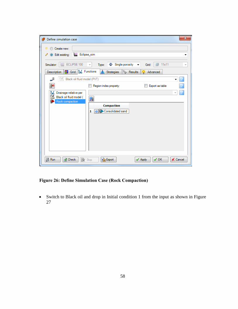
Switch to Rock Compaction and drop in Consolidated sand from the input as shown
in Figure 26
58
Figure 26: Define Simulation Case (Rock Compaction)
Switch to Black oil and drop in Initial condition 1 from the input as shown in Figure
27
59
Figure 27: Define Simulation Case (Initial Condition)
Switch to Strategy tab
Use the insert button to add a row to the table
Select Development strategy1 and drop into Development strategy as shown in
Figure 28
60
Figure 28: Define Simulation Case (Development Strategy)
Click Export button to export the simulation case
Click the Run button (Run your project from the C-drive)
Results
Open a New function window
On the Cases tab check the box next to Eclipse_sim
Open Results tab check Well under the identifier folder and select Wells
P1,P2,P3 and P4 under the PROD folder
Select Dynamic Data
61
Open the Dynamic results data folder and the Rates folder
Check the Oil production rate checkbox to plot the oil production rates for all 4
producers.
Open another function window and repeat the process to plot the Water
production rate.
Figure 29: Oil Production Rates for the 4 Producers with Eclipse 100
64
Figure 32: Water Saturation Map at 200 days with Eclipse 100
Figure 33: Pressure Map at 100 days with Eclipse 100
65
Figure 34: Pressure Map at 200 days with Eclipse 100
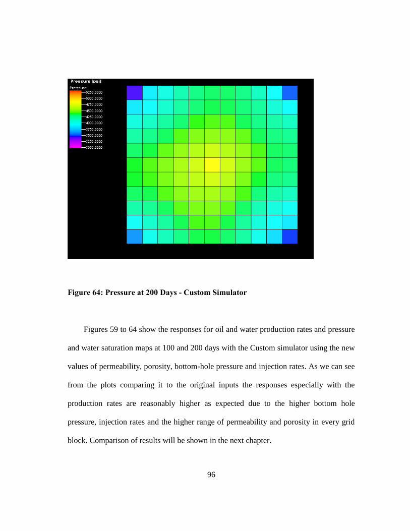
Figures 29 to 34 show the responses obtained using Eclipse100 for oil and water
production rates up till the end of simulation time, water and pressure saturation maps at
100 and 200 days. As expected, within a considerable amount of time we have water
breakthrough and the oil and water production rates increase significantly with the water
production rates leveling off and the oil production declining quite steeply after a while.
The water saturation and pressure maps in both cases increase with increasing time away
from the injector as expected exhibiting the typical performance of a water flood pattern.
In the next chapter, we cover the topic of Petrel extension via Ocean Software
Development Kit and show in general terms how Petrel can be extended with respect to
66
the motivation of this project using our in-house two phase two dimensional oil water 5-
spot pattern water flood simulation configuration as the model to establish the
framework for Petrel extension.
67
CHAPTER IV
OCEAN IN PETREL AND CUSTOM SIMULATOR
Ocean in Petrel
Ocean in Petrel is an application programming interface that is used by a
software developer to extend the functionality of Petrel, the pre and post processor of
Eclipse by creating plug-ins which contains algorithms designed by developers to
implement unique objectives. The software developer can be a member of academia,
industry or a separate third party that has identified a need to extend the features of
Petrel for their personal benefit or with the purpose of making their plug-ins available
commercially for interested parties. The software developer is able to create plug-ins by
making use of different Ocean templates (Figure 34) that are available in Visual Studio
which is the programming environment through which Ocean and Petrel communicate.
The user of Ocean in Petrel has access to common services such as service
locator, messaging interface, module lifecycle, data source manager, event transaction
manager, domain object hosting, generic data types etc. With the ocean software
development kit, the developer has the ability to “unleash their creativity” and extend the
user interface of petrel, manipulate data and add to the workflow of model building with
the numerous tools and services that give them access to the various domains in Petrel
such as seismic domain, well domain, geology, shapes, reservoir model, simulation etc.
The basic building block of a plug-in is the module which is self-contained in
assembly. The modules which contain the algorithms to extend the Petrel data user
interface are loaded at Petrel start up and unloaded at shut down. The module goes
68
through five steps in its life cycle namely initialize, integrate, integrate presentation,
disintegrate and dispose.
The features of ocean and its capability are far too extensive to be covered in this
project so for a more comprehensive coverage of Ocean in Petrel Software Development
Kit, I refer you to attend the class thought by the software owners i.e. Schlumberger by
registering for a session through the company website “www.ocean.slb.com.”
At this time, I need to remind the reader of the general objective of this project
which is to develop a framework for adding our developed algorithms in the form of
“processes” to the workflow of Petrel for model building to prepare “cases” for reservoir
simulation. For our purposes, there are two primary ways of accomplishing this goal.
One is through what is referred to as a “workstep” which has its algorithm self-contained
in a module that on execution will implement the code in the module. Depending on
what the algorithm is designed to do, it could accept inputs and pass the inputs through
the algorithm and produce outputs that could be used for further processing. The other
suggested method which is the preferred method is the implementation of a custom
simulator which will accept inputs in a certain format to be fed to a custom simulator
which is passed through its algorithm and returns responses back to Petrel workspace for
visualization. Presently in Petrel we have available to us four simulators i.e. Eclipse 100,
Eclipse 300, FrontSim and INTERSECT. Ocean in Petrel gives the user the ability to
add a custom simulator to the drop box in the “define simulation case” window of Petrel.
For completion, I will talk about the general flow in developing plugs-in with an
example that will give a sense of the workflows and then I will concentrate on the
69
implementation of the custom simulator. Figure 35 below shows the Petrel user interface
with the different forms in which personalized algorithms and their responses could be
added. They include processes/worksteps, data models, menus, windows, toolbars,
dialogs 2D and 3D renderers etc.
Figure 35: Petrel User Interface (Adapted from Ocean Software Development Kit
Fundamental Training Volume 1)
70
After Ocean and Petrel have been installed, the process of developing plug-ins in
Petrel begins with selecting the appropriate Ocean template in Visual Studio which is the
programming environment for interaction between Ocean and Petrel. Figure 36 below
shows the choices of templates that can be chosen to implement your algorithms.
Figure 36: Ocean Templates in Visual Studio
How to Make a Plug-in
Once a choice is made, a wizard is opened which guides the developer through a
series of steps to assist them to generate generic blocks of code that are needed to
implement their algorithms. As an example, I will implement in the next section a plug-
71
in that will add a workstep to Petrel to display the name of the active project opened in
Petrel.
Making Ocean Plug-ins
Open up Visual Studio 2010
Select OceanPlugin as the template as shown in Figure 37
Give it a name and location
Click Ok
Figure 37: Choosing Ocean Template
72
In the wizard that shows after clicking Ok, enter the relevant information as
shown below in Figure 38.
Figure 38: Ocean Plug-in Create - Step 1
Click Next and next again
In the next steps, fill the information as shown in figure 39, 40 and 41below
Click Next and then Finish
74
Figure 41: Ocean Plug-in Create - Step 5
After going through these steps the ocean wizard will create a project in Visual
Studio that will have a plug-in as a project and a module with a workstep attached to it.
An instance of a plug-in and module are shown in Figures 42 and 43 respectively. The
wizard has been designed to do a lot of the setting up for developers leaving the
customization based on the desired objectives of the workstep (plug-in) for the developer
to fill in. To complete the wizard, on the last page that comes up, check the “Additional
Reference Settings” box to add the relevant assemblies to the project solution. These
assemblies can be found in the Petrel 2012 folder in the Schlumberger folder in the
“Programs” folder.
76
For most customization in Petrel, the most important part of customizing
modules is the code placed in the “ExecuteSimple ()” Method as shown in Figure 44. It
is in this block that the developer places their algorithm for Petrel extension.
Click on OceanModuleWorkstep.cs in the Solution Explorer window
Figure 44: ExecuteSimple Method
Build project in Visual Studio
Open Petrel
Click on Processes pane (Bottom Left) and open Plug-ins
Double click on OceanModuleWorkstep and then Apply/OK
77
Figure 45: OceanModuleWorkstep
Since no project is open you will get the default value i.e. “No project is open” as
shown in Figure 45. If a project is opened, then it will display the project name. As
simple as this example is, it shows the basics in developing plug-ins by utilizing the
wizard to generate most of the code that is used with the relevant parts to be customized
according to your objectives. With a workstep, inputs can be passed to the
“ExecuteSimple” method for processing to produce outputs that could be used further
78
for model building. In the next section, I describe the development of our custom
simulator.
Custom Simulator
Being able to develop a custom simulator to add to the choices of simulators
available is a very useful resource of Ocean. Granted that the present simulators Eclipse
100, 300 etc. are very powerful but in certain instances, a certain level of customization
is needed to achieve our objectives. This project began with a certain motivation in mind
which was to develop a framework for creating a means to implement custom algorithms
in the areas of model order reduction and production optimization. In order to achieve
our goal, a test model was used to develop a custom simulator i.e. a two phase two
dimensional 5-spot pattern waterflood. For propriety reasons, certain parts of the code
implementing the custom simulator cannot be shown here but the general steps to
develop the simulator will be explained below with a few figures to give a visual of the
process.
The process of developing the custom simulator began with calibrating our test
model which was earlier programmed in Matlab (for prototyping) against the same
reservoir simulation algorithm re-programmed in C-sharp which is the language of
Ocean. After calibration was completed, in collaboration with a Schlumberger software
development team, I was able to add a custom simulator to the choices of simulators in
the “define simulation case” dialog box of Petrel and develop our framework for custom
simulator building.
79
As displayed in Chapter 3 with the implementation of our test model in Petrel,
the prepared “case” is developed by going through a series of actions to complete the
description needed to come up with a scenario for reservoir simulation. It begins with
making a simple grid, making horizons, layering, creating properties like porosity and
permeability, selecting a fluid model, selecting rock physics functions, adding wells and
constraining those wells, creating a development strategy and finally defining the case
and submitting it to a choice of reservoir simulators (in this case Eclipse 100) for
simulation. Figure 46 below shows the process of reservoir simulation in Petrel with
regard to our test case.
Figure 46: Reservoir Simulation in Petrel (Slide Courtesy of Schlumberger)
80
After the case has been defined in “define simulation case” and submitted for
reservoir simulation, the case is ran and then on completion the results are imported back
into Petrel for visualization. To make a custom simulation, the flow process is not so
different. In order to give the developer the opportunity to add their functionality, a
series of steps are included in order to customize and format the custom simulator into a
well suited form. Figure 47 below captures the additional steps implemented for
customization.
Figure 47: Process for Developing a Custom Simulator
Simulator runs
Simulator
Petrel imports Eclipse format
Case exported in Eclipse PostExport (Case)
PreRun(Case)
PreImport(Case)
SubmitCommand
User defines case
81
The steps of note are the PostExport, PreRun, PreImport and SubmitCommand.
For each of these additional steps it’s the place where the developer can add the
customized functionality they want. For instance in the PostExport(Case) method, the
deck that is exported from the define simulation case is reformatted and modified in a
form that the custom simulator expects. The PreRun sets up the environment before the
simulation launch. The submit command submits the case to the simulator and the
PreImport method formats the results from the simulator in an Eclipse format suited for
visualization in Petrel. The reservoir simulation code was developed by the author and
the connection with Petrel was developed by a Schlumberger software developer. Figure
48 below shows a snap shot of the custom simulator “Student Simulator” added to the
drop list of simulators.
Figure 48: Student Simulator in Define Simulation Case
82
As mentioned, for propriety reasons certain parts of the code cannot be shown
but the general framework for connecting the reservoir simulator to Petrel is shown
below with a few visuals. I draw the attention of the reader to Figure 49 below that
shows the “Student Simulator” i.e. our custom simulator. When this choice is selected
from the simulator drop list, an additional tab named “Custom tab” appears.
Figure 49: Student Simulator and Custom Tab
When the user clicks on the “Custom tab” tab in order to submit their “simulation
file they would need to have pre-built (compiled) their reservoir simulation solution in
Visual Studio to generate a “dll” file that will be uploaded using the “Browse Simulator”
83
button shown in the figure above. The custom simulator has been developed such that
certain parts such as the code for the PostExport, PreRun, SubmitCommand and
PreImport methods are sealed but the parts that can be shown are displayed below.
In order to generate the “dll” to be passed to the custom simulator, the user has to
prepare a reservoir simulation file in the format shown in Figure 50 below.
Figure 50: Format of the Code to Generate Dll File
Also specific to generating the dll file the user has to follow the instructions as
stated below.
Please follow the instructions for locating *.dll file. /// --Program Template: the following must exist in this program with the exact names /// 1. the namespace with the name: "SimDllFile"
84
/// 2. The namespace must contain three classes: "SimClass","InputArgs","OutputArgs" /// 3. "SimClass" should contain a public method named "Simulate" of the form: public OutputArgs Simulate(InputArgs inputs) /// This method is the place for writing the simulator's computations. Note that /// in the following example "RunSimulatorMethod" is a private method that is called by "Simulate" method. "RunSimulatorMethod" /// method is NOT a part of presumed structure. The developer can have any number of private methods to be called from "Simulate" method. /// /// --Where to locate *.dll file: /// 1. press F6 to build the *.files. The file that should be loaded by simulator is "SimDllFile.dll" and is copied at C:\StudentSimulator. /// or ...Documents\StudentSimulator. /// /// --Note: before creating *.dll file, with the explained structure, make sure that your simulator runs, independently. You could test this in a console application with constant inputs.
The inputs in the “Input region” in the code shown are passed from Petrel to the
reservoir simulator in the format shown in Figure 51 below which is compatible with
Eclipse to be used in the “Computation region” of the code which is where
transmissibility, sources and sink terms and accumulation matrices are calculated, the
set of equations are solved using an iterative solver, the oil and water production rates
for the producers and “lists” containing pressure and water saturation values for every
grid block at every time step to be converted to maps at every time step are stored for
visualization at the end of simulation with the “RunSimulatorMethod” method.
85
Figure 51: Format to Pass Inputs from Petrel to Custom Simulator
Of note in my program are two methods i.e. Saturation_OilPressureDependencies
and RunSimulatorMethod. Both perform two separate functions. The first calculates the
water and oil relative permeability as a function of water saturation for every grid block
and also the oil viscosity and formation volume factor as a function of pressure all at
every time step. This function is basically an interpolation function that accepts the
values for saturations and pressures for every grid block as inputs and parses out
interpolated values of relative permeability, viscosity and formation volume factors to be
used in calculations in the Computation region. The second method i.e.
RunSimulatorMethod is the method used to store oil and water production rates, pressure
86
and saturation values in every grid block at every time step to be passed back to Petrel
workspace for visualization. The block of code below shows the RunSimulationMethod
in its entirety as shown in Figure 52 below which after simulation is completed, stores
the oil and water production rates for all the well, pressure and saturations for every grid
block at every timestep to be imported via a connection into Petrel for visualization.
private static OutputArgs RunSimulatorMethod(InputArgs Inputs, double[,] qo_qw, double[,] Po_Sw_Values) { // Production Rates List<double> _Producer1_oilratevector = new List<double>(); // for recording Oil Production Rate of Producer 1 List<double> _Producer1_waterratevector = new List<double>(); // for recording Water Production Rate of Producer 1 List<double> _Producer2_oilratevector = new List<double>(); // for recording Oil Production Rate of Producer 2 List<double> _Producer2_waterratevector = new List<double>(); // for recording Water Production Rate of Producer 2 List<double> _Producer3_oilratevector = new List<double>(); // for recording Oil Production Rate of Producer 3 List<double> _Producer3_waterratevector = new List<double>(); // for recording Water Production Rate of Producer 3 List<double> _Producer4_oilratevector = new List<double>(); // for recording Oil Production Rate of Producer 4 List<double> _Producer4_waterratevector = new List<double>(); // for recording Water Production Rate of Producer 4 // Pressures and Water Saturations List<double[, ,]> _pressuregridvector = new List<double[, ,]>(); // for recording Pressure Calculations List<double[, ,]> _watersaturationridVector = new List<double[, ,]>(); // for recording Water Saturation Calculations //.............for storing pressures and saturations while looping //+++++++++++++ looping through all the time steps
Figure 52: RunSimulationMethod Code
87
int rowshifter = 0; int pressurecolumnshifter = 0; int watersaturationcolumshifter = 1; for (int i = 0; i < Inputs.ReportingTimes.Count; i++) { //................ Calculating Oil and Water Production Rate Vectors _Producer1_oilratevector.Add(qo_qw[i, 0]); _Producer1_waterratevector.Add(qo_qw[i, 1]); _Producer2_oilratevector.Add(qo_qw[i, 2]); _Producer2_waterratevector.Add(qo_qw[i, 3]); _Producer3_oilratevector.Add(qo_qw[i, 4]); _Producer3_waterratevector.Add(qo_qw[i, 5]); _Producer4_oilratevector.Add(qo_qw[i, 6]); _Producer4_waterratevector.Add(qo_qw[i, 7]); double[, ,] PressureGrid = new double[Inputs.Nx, Inputs.Ny, Inputs.Nz]; double[, ,] WaterSaturationGrid = new double[Inputs.Nx, Inputs.Ny, Inputs.Nz]; Figure 52 for (int ii = 0; ii < Inputs.Nx; ii++) { for (int j = 0; j < Inputs.Ny; j++) { for (int k = 0; k < Inputs.Nz; k++) { PressureGrid[ii, j, k] = Po_Sw_Values[rowshifter, pressurecolumnshifter]; WaterSaturationGrid[ii, j, k] = Po_Sw_Values[rowshifter, watersaturationcolumshifter]; rowshifter = rowshifter + 1; } } } rowshifter = 0; pressurecolumnshifter = pressurecolumnshifter + 2; watersaturationcolumshifter = watersaturationcolumshifter + 2; //..........Adding the Grids list _pressuregridvector.Add(PressureGrid); _watersaturationridVector.Add(WaterSaturationGrid); } //+++++++++++
Figure 52: Continued
88
// returning the ouputs OutputArgs Outputs = new OutputArgs(); Outputs.Producer1_OilRateVector = _Producer1_oilratevector; Outputs.Producer1_WaterRateVector = _Producer1_waterratevector; Outputs.Producer2_OilRateVector = _Producer2_oilratevector; Outputs.Producer2_WaterRateVector = _Producer2_waterratevector; Outputs.Producer3_OilRateVector = _Producer3_oilratevector; Outputs.Producer3_WaterRateVector = _Producer3_waterratevector; Outputs.Producer4_OilRateVector = _Producer4_oilratevector; Outputs.Producer4_WaterRateVector = _Producer4_waterratevector; Outputs.PressureGridVector = _pressuregridvector; Outputs.WaterSaturationGridVector = _watersaturationridVector; return Outputs; } }
Figure 52: Continued
As part of the motivation of this project, the final product will be used in the class
room environment for educational purposes where students will be given the inputs used
to develop the case as presented here in this project and develop a reservoir simulator
that will be connected via ocean to Petrel to match the responses of the Eclipse100
equivalent simulated case. We ran the Student Simulator with the same inputs and
obtained figures 53 to 58 for the responses for oil and water production rates and water
and pressure maps.
90
Figure 54: Water Production Rate Using Custom Simulator
Figure 55: Water saturation at 100 Days with Custom Simulator
91
Figure 56: Water Saturation at 200 Days with Custom Simulator
Figure 57: Pressure Map at 100 Days with Custom Simulator
92
Figure 58: Pressure Map at 200 Days with Custom Simulator
The above plots show the responses for oil and water saturation up till the end of
simulation time, pressure and water saturation maps at 100 and 200 days using the
custom simulator. In a similar fashion as the Eclipse100 simulation run shown in chapter
three, the custom simulator exhibits similar responses in performance. The custom
simulator in its present form can accept various operating parameter values for
permeability, porosity, well constraints (bottom-hole pressures for producers and rates
for injectors) etc. Figures displaying the oil and water production rates and the pressure
and water saturation maps with the following values are shown
93
- Permeability (randomly generated with min of 100md and max of 400md)
- Porosity of 0.35
- Bottom-Hole Pressure of 3200 psi
- Injection rate 4,500 STB/day
Figure 59: Oil Production Rates - Custom Simulator
94
Figure 60: Water Production Rates - Custom Simulator
Figure 61: Water Saturation at 100 Days - Custom Simulator
95
Figure 62: Water Saturation at 200 Days - Custom Simulator
Figure 63: Pressure at 100 Days - Custom Simulator
96
Figure 64: Pressure at 200 Days - Custom Simulator
Figures 59 to 64 show the responses for oil and water production rates and pressure
and water saturation maps at 100 and 200 days with the Custom simulator using the new
values of permeability, porosity, bottom-hole pressure and injection rates. As we can see
from the plots comparing it to the original inputs the responses especially with the
production rates are reasonably higher as expected due to the higher bottom hole
pressure, injection rates and the higher range of permeability and porosity in every grid
block. Comparison of results will be shown in the next chapter.
97
CHAPTER V
COMPARISON OF RESULTS AND CONCLUSIONS
In this chapter, I compare the results obtained from using Eclipse100 and the
custom simulator for accuracy and error analysis. The analysis is conducted by
comparing the results of two cases, one which makes use of a homogenous permeability
of 100md and the other which is a heterogeneous permeability case used in developing
our framework; both cases of which are five-spot water flood pattern configured.
I compare the results on a well by well basis for oil and water production rates
visually and present a table with root mean square error for each well. The error analysis
will be followed by interpretations based on the results of the simulations and at the end
I make my conclusions and recommendations.
Root Mean Square Error Analysis
Figures 65 to 68 show the oil and water production rates for the homogenous case.
98
Figure 65: Oil Production Rate of P1 with both Simulators (Homogeneous Case)
Figure 66: Water Production Rate of P1 with both Simulators (Homogeneous Case)
99
Figure 67: Oil Production Rate of P2 with both Simulators (Homogeneous Case)
Figure 68: Water Production Rate of P2 with both Simulators (Homogeneous Case)
100
Since this first case is homogeneous, all four producers have the same
performance of oil and water production rates so figures for Producers three and four are
not shown. Visually it can be seen that the oil and water production rates using
Eclipse100 and the Custom Simulator match for all wells. Below is a table showing the
root mean square error calculated with the expression below.
√
(44)
Where
Ql_eclipse is the production rate of oil or water at a particular time using Eclipse100
Ql_customsimulator is the production rate of oil or water at a particular time using the custom
simulator
n is the number of reported values
RMS ERROR AT END OF SIMULATIOM
OIL PROUCTION
RATE(STB/D)
WATER PRODUCTION
RATE (STB/D)
PRODUCER 1 25 17
PRODUCER 2 25 17
PRODUCER 3 25 17
PRODUCER 4 25 17
Table 4: Rms Error of Production Rate for all Producers (Homogenous Case)
From Table 4 above, the root mean square error for both oil and water production
rate for all producers for this case of homogenous permeability is notable which is rather
misleading because visually, the oil and water production rates match very well. I
101
attribute this root mean square error value to the values reported at different times for the
Eclipse100 and Custom Simulator runs which might be as a result of the manner in
which values are reported for the Custom Simulator and quite possibly internal
computations peculiar to Eclipse that the Custom Simulator doesn’t account for. I
analyzed the performance of the heterogenous permeability case for both simulators and
obtained Figures 69 to 76 below showing the oil and water production rates.
Figure 69: Oil Production Rate of P1 with both Simulators (Heterogenous Case)
102
Figure 70: Water Production Rate of P1 with both Simulators (Heterogenous Case)
Figure 71: Oil Production Rate of P2 with both Simulators (Heterogenous Case)
103
Figure 72: Water Production Rate of P1 with both Simulators (Heterogenous Case)
Figure 73: Oil Production Rate of P3 with both Simulators (Heterogenous Case)
104
Figure 74: Water Production Rate of P3 with both Simulators (Heterogenous Case)
Figure 75: Oil Production Rate of P4 with both Simulators (Heterogenous Case)
105
Figure 76: Water Production Rate of P4 with both Simulators (Heterogenous Case)
Visually, the oil and water production rates for all wells of this heterogenous case
obtained using Eclipse100 and the Custom Simulator are also matched quite well with
the exception of the water production rate curves for Producers two and three which has
a maximum water production rate point error of five percent. Table 5 below shows the
root mean square error of oil and water production rates for all Producers.
RMS ERROR AT END OF SIMULATION
OIL PROUCTION
RATE(STB/D)
WATER PRODUCTION
RATE (STB/D)
PRODUCER 1 22.3 10.3
PRODUCER 2 28 38
PRODUCER 3 14 43
PRODUCER 4 24 9.24
Table 5: Rms Error of Production Rate for all Producers (Heterogenous Case)
106
Similarly to the homogenous case, the root mean square error for each well
comparing the oil and water production rates is misleading since from just visually
inspecting the rates, we expect to see a much smaller root mean square error. I attribute
this difference again to the manner in which the reporting values are obtained between
both simulators and the internal computation done by Eclipse to calculate responses
based on its algorithm.
At this point, I have established that the responses using oil and water production
rates match reasonably well bearing in mind that in order to understand the difference in
reported values, a reasonable amount of time has to be spent understanding the subtle
differences between the computations done by Eclipse and how it differs from that of the
Custom Simulator.
Pressure and Time-Step Analysis
Between both cases i.e. the homogenous and heterogenous cases, we have a
reasonable match but to see if we can quantify further the differences, two more
situations are investigated. Firstly, a comparison between the pressures in every grid
block at random time steps during simulation obtained from Eclipse100 and the Custom
Simulator using root mean square error analysis and secondly, a time step reduction to
account for the difference in partial difference equation formulation and solving method
since Eclipse is a fully implicit simulator and the custom simulator is formulated using
lagging coefficient. For this second case, the time step of the custom simulator will be
reduced from 0.2 days to 0.001 days and the results will be compared against the
107
Eclipse100 results for the heterogenous case; specifically the oil and water production
rates of Producers two and three which seemed to have the highest discrepancy.
To conduct the pressure analysis, the pressures in every grid block at different time
steps capturing the performance of the entire simulation are compared. Figures 77 to 81
below show a comparison of pressures at different time steps.
Figure 77: Pressures from Eclipse 100 and Custom Simulator on February 15th
0
500
1000
1500
2000
2500
3000
3500
4000
4500
5000
0 50 100 150
Pre
ssu
re (
psi
)
Grid Number
Pressure Analysis_02_15
Pressure_02_15_EclipsePressure_02_15_Sim
108
Figure 78: Pressures from Eclipse 100 and Custom Simulator on April 15th
Figure 79: Pressures from Eclipse 100 and Custom Simulator on June 15th
0
500
1000
1500
2000
2500
3000
3500
4000
4500
5000
0 50 100 150
Pre
ssu
re (
psi
)
Grid Number
Pressure Analysis_04_15
Pressure_04_15_Eclipse
Pressure_04_15_Sim
0
500
1000
1500
2000
2500
3000
3500
4000
4500
5000
0 50 100 150
Pre
ssu
re (
psi
)
Grid Number
Pressure Analysis_06_15
Pressure_06_15_EclipsePressure_06_15_Sim
109
Figure 80: Pressures from Eclipse 100 and Custom Simulator on August 15th
Figure 81: Pressures from Eclipse 100 and Custom Simulator on October 1st
0
500
1000
1500
2000
2500
3000
3500
4000
4500
5000
0 50 100 150
Pre
ssu
re (
psi
)
Grid Number
Pressure Analysis_08_15
Pressure_08_15_Eclipse
Pressure_08_15_Sim
0
500
1000
1500
2000
2500
3000
3500
4000
4500
5000
0 50 100 150
Pre
ssu
re (
psi
)
Grid Number
Pressure Analysis_10_1
Pressure_10_1_EclipsePressure_10_1_Sim
110
The Table below shows how the Custom Simulator performs in comparison to
Eclipse100 using root means square error analysis with the following expression.
√
(45)
Where
Pl_eclipse is the pressure of oil or water at a particular time using Eclipse100.
Pl_customsimulator is the pressure of oil or water at a particular time using the custom
simulator.
n is the number of reported values.
PRESSURE (ROOT MEAN SQUARE ERROR)
February 15th April 15th June 15th August 15th October 1st
339 psi 780 psi 540 psi 467 psi 431 psi
Table 6: Pressure Rms Analysis between Both Simulators (Heterogenous Case)
From the pressure plots above it can be inferred that the custom simulator shows a
similar pattern of performance to the Eclipse100 simulator. From inspection, it seems
that Eclipse probably makes use of some kind of multiplier which the Custom Simulator
doesn’t factor in. The root mean square error analysis in Table 6 above gives a measure
of the average difference between the pressures between both simulators at different
time steps during simulation. Following the analysis of the second case with a reduced
111
time step, I will make my final observations, conclusions and recommendations
concerning my analysis.
For my last scenario of investigation, I reduced the time step. For a lagging
coefficient formulated simulator, the biggest issue dealt with is that of stability. In order
to ensure stability, the simulator can only march in time at or below a certain threshold
which for this simulator is 0.2 days and so we have this time step constraint. It is
expected that if the time step of a lagging coefficient simulator is reduced orders of
magnitude lower than the threshold, results obtained will be in closer agreement with a
fully implicit simulator such as Eclipse but from the analysis presented thus far it would
seem the discrepancy between both Eclipse and the Custom simulator lies more within
the internal computations of Eclipse that the Custom Simulator doesn’t account for. For
investigating purposes and completeness, the time step was reduced to 0.001 days to see
if results are improved. Figures 82 to 85 below show the oil and water production rates
of Producers two and three followed by a root mean square error analysis table.
112
Figure 82: Oil Production Rate of P2 with Custom Simulator (0.001 days)
Figure 83: Water Production Rate of P2 with Custom Simulator (0.001 days)
113
Figure 84: Oil Production Rate of P 3 with Custom Simulator (0.001 days)
Figure 85: Water Production Rate of P3 with Custom Simulator (0.001 day)
114
RMS ERROR AT END OF SIMULATION
OIL PROUCTION
RATE(STB/D)
WATER PRODUCTION
RATE (STB/D)
PRODUCER 2 (0.2 days) 28 38
PRODUCER 3 (0.2 days) 14 43
PRODUCER 2 (0.001 days) 5 38
PRODUCER 3 (0.001 days) 3.2 43.2
Table 7: Rms Analysis of Production Rate at 0.001 and 0.2 Timesteps for P2 and P3
From the plots above, it can be seen visually that the oil and water production
rates obtained with the lower timestep of 0.001 gives a very similar performance to the
0.2 timestep simulation. It is also seen from table 7 with the root mean square error
analysis at the end of simulation that the oil production rate obtained with the custom
simulator converges with Eclipse while the water production rate does not. Water break
through occurs at approximately 14 days into the simulation which is also the time oil
production begins to decline rapidly. It is possible that with lower timesteps, the oil
production rates my match even much better but there is no indication that the water
production rate will improve any better. Thus far in my analysis, I have attributed the
mismatch to internal computations in Eclipse that are not considered in the custom
simulator and perhaps the formulation method and have so far seen no indications to
convince me otherwise.
115
Recommendation
With all the analysis done comparing the performance of the Custom Simulator
for both homogenous permeability and heterogenous permeability case to the Eclipse
run, the mismatch between both simulators is more apparent for the heterogenous case
especially for the water production of Producers two and three. Analyzing the
distribution of pressures in each grid block at different timesteps as shown in figures 77
to 81the argument of internal computations in Eclipse is supported because of the pattern
exhibited indicating that there probably is a multiplier applied in Eclipse that is
responsible for the upward shift in pressures. The objective of this thesis which is to
develop a framework for extending Petrel has been achieved. The plug-in its present
form is ready to be used in a classroom environment as part of the tools in educating
students on reservoir simulation. Matching the performance of Eclipse is definitely an
objective of ours but to match Eclipse fully, a considerable amount of time has to be
spent in understanding its internal computations. After that study has been conducted,
findings can be implemented in future versions of the plug-in. Also it is recommended
that the plug-in be upgraded to a fully implicit formulated simulator not only to obtain
results much closer to Eclipse but to compare the performance between a lagging
coefficient simulator and a fully implicit simulator. In the next section, I present plans
for future work and make my final conclusions.
Future Work and Conclusion
Reservoir simulation is continuously developing with the tools and methods for
reservoir simulation becoming more efficient and accurate. We began this project with
116
the goal in mind to ultimately make our contribution to reservoir simulation
development in general by first identifying and working to improve on results obtained
in the past in certain areas of interest. Efficient and robust algorithms for areas such as
model order reduction and production optimization are in progress and with the work
accomplished in this project, when these algorithms are completed, similar custom
simulators will be built to implement the algorithms.
Regarding future work, the extent of this project is very far reaching. We have
accomplished our goal of establishing our framework for extending Petrel via a custom
simulator with Ocean. The test model that we used was a very simple shoe box model.
As I mentioned in my introduction, we currently deal with very complex reservoir
systems that require the use of unstructured grids. This is one area where our plug-in
could be improved to better accommodate more realistic reservoir scenarios. The
configuration that we used was fixed i.e. a five-spot pattern with wells placed in a fixed
position. The code could be altered to allow for more flexibility of well placement and
well constraint. Lastly, Ocean gives the software developer access to every domain in
reservoir modeling. Future plug-ins made might have influences from other domains of
model building such as geology, geophysics etc. The software developer is only limited
by their creativity so the possibilities for improvements are endless. And lastly, in
connection with the result comparison chapter, to model more realistic scenarios using
Eclipse as a basis, studies have to be conducted to factor into the Custom simulator the
internal computations that are representative of real life reservoir performance.
117
In conclusion, we have taken a first step to accomplish our ultimate goal. With
this project, as it is firstly academic, it will be used in a class room environment. It will
be of immense value to students because it will help them in getting a stronger
understanding of fundamental and advanced topics in reservoir simulation. The other
aspect is its research component which is tied to the future plug-ins to be made in our
identified areas of model order reduction and production optimization. The algorithms
for these areas are currently developed and when completed, custom simulators will be
developed to implement them.
118
REFERENCES
Antoulas A.C., 2005. Approximation of Large-Scale Dynamical Systems, SIAM,
Philadelphia.
Blackwell, R.J. and Richardson, J.G. 1971.Use of Simple Mathematical Models for
Predicting Reservoir Behavior. Paper SPE 2928 was presented at SPE 45th
Annual Fall Meeting, Houston, Texas.
Chen, Y., Durlofsky, L.J., and Wen, X.-H. 2005. Efficient Three Dimensional
Implementation of Local-Global Upscaling for Resrvoir Simulation.
Paper SPE 92965.
Christie, M.A. 1996. Upscaling for Reservoir Simulation. Paper SPE 37324
ECLIPSE Reservoir Engineering Software. 2012. Schlumberger,
http://www.slb.com/content/services/software/reseng/eclipse.aspx.
Ertekin, T., Abou-Kassem, J.H., and King, G.R. 2001. Basic Applied Reservoir
Simulation. Spe Textbook Series. Richardson, Tex.: Society of Petroleum
Engineers.
Gildin, E., Klie, H., Wheeler, M.F., Rodriguez, A., and Bishop, R.H. 2006. Projectio-
based Approximation Methods for the Optimal Controlof Smart Fields. In
Proceedings of the 10th
European Conference on the Mathematics of Oil
Recovery. Amsterdam, The Netherlands, September 4-7
Gildin, E., Lopez, T.J. 2011. Closed-Loop Reservoir Management: Do We Need
Complex Models?. Paper SPE 144336.
Hoang, M.T., Satter, A., and Varnon, J.E. 1992 Integrated Reservoir Management. Paper
22350 was presented at the 1992 SPE International Meeting on Petroleum
Engineering, Beijing China.
Matlab, R2012b. Natick, Massachusetts: The Mathworks, Inc.
Ocean Software Development Kit, Fundamentals Training 2012 Volumes 1, 2 and 3,
Version 2011.1. Schlumberger Information Solutions.
Petrel Reservoir Engineering Software. 2012. Schlumberger,
http://www.slb.com/content/services/software/resent/.
Schlumberger, 2012. Ocean Store.
http://www.ocean.slb.com/Pages/default.aspx (Accessed 25 February 2012)