Extensions of Cox Model for Non-Proportional Hazards Purpose

Brussels 13th - 16th October 2013

Author: Jadwiga Borucka PAREXEL, Warsaw, Poland

PhUSE Annual Conference 2013

Paper SP07

Presentation Plan 1.Introduction - Cox model definition 2.Proportional hazard assumption 3.Sample dataset 4.Verification of PH assumption 5.Interactions with function of time 6.Stratified model 7.Conclusions

INTRODUCTION – COX MODEL DEFINITION

The first semi-parametric model was proposed by Cox (1972) who assumed that the covariates-related component is distributed exponentially The covariates-related component is expressed as exp(βx), thus the model has the following formula:

Where: – hazard function that depends on timepoint t and vector of covariates x – baseline hazard function that depends on time only – covariates-related component

PROPORTIONAL HAZARD ASSUMPTION Comparing hazard between two subjects at time t via HAZARD RATIO: Subject (1) – covariates: x = x1 Subject (2) – covariates: x = x2

HR (hazard ratio) – proportion of hazard function value for two subjects wit different values of covariate(s) at the given timepoint t

HR does not depend on time (on covariates only) λ0(t) – baseline hazard function does not have defined mathematical formula

PROPORTIONAL HAZARD ASSUMPTION

Proportional hazard assumption – discussion

Violation does not cause serious problems as in such cases parameter estimate

can be interpreted as  ‘average  effect’   of the covariate

(e.g. Allison, 1995)

Violation should be taken into account and appropriate modification of the model

should be used to enable more precise interpretation

(e.g. Hosmer, Lemeshow, 1999) example of study site in clinical trial for which

it is very likely that the assumption will be violated

SAMPLE DATASET Data for 60 patients from open-label clinical trial on safety of newly invented therapy for brain cancer AGE = Age at screening SITE = Number of study site (SITE = 1 stands for Site B, SITE = 2 stands for Site A) TIME = Time (in days) from the beginning of therapy till death (if patient dies) or till the end of the observational period (if patient survives) CENSOR = Indicator of the event (CENSOR = 1 stands for death of patient, CENSOR = 0 stands for survival till the end of the observational period)

VERIFICATION OF PH ASSUMPTION

Proprotional hazard assumption – methods of verification

plot  of  ‘log-negative-log’  of  the  Kaplan-Meier estimator of survival function:

curves on the plot should be pararell with distance that is constant over time

plot of Schoenfeld residuals as a function of time:

residuals should not show any trend

adding interaction of a covariate with function of time variable: newly added variable should not be

statistically significant

VERIFICATION OF PH ASSUMPTION Proportional hazard assumption for the Cox model estimated for 60 subjects from the open-label study: Step 1 Model estimation – time to death is being analyzed, AGE and SITE included as covariates

Both variables statistically significant, confidence interval for hazard ratio for AGE does not include 1, for SITE however confidence interval includes 1, which means that there might be no difference between two study sites

in terms of risk of dying

VERIFICATION OF PH ASSUMPTION Step 2 Verification of proportional hazard assumption for AGE Plot of Schoenfeld residuals vs time

Residuals do not show any trend,

smoothed line has approximately 0 slope, which indicates that

proportional hazard assumption

is satisfied for AGE

VERIFICATION OF PH ASSUMPTION Step 2 Verification of proportional hazard assumption for AGE – cont.

Adding interaction of AGE by TIME to the model

Newly added variable is not statistically significant which indicates that proportional hazard

assumption is satisfied for AGE

VERIFICATION OF PH ASSUMPTION Step 3 Verification of proportional hazard assumption for SITE Plot of Schoenfeld residuals vs time

Residuals do not give straightforward answer, however they

might suggest violation from PH assumption for SITE

VERIFICATION OF PH ASSUMPTION Step 3 Verification of proportional hazard assumption for SITE – cont. Adding interaction of SITE by TIME to the model

Interaction of SITE by TIME is significant at the level of 0.1 which may lead to the conclusion that proportional hazard

assumption is likely to be violated for SITE

VERIFICATION OF PH ASSUMPTION Step 3 Verification of proportional hazard assumption for SITE – cont. Plot  of  ‘log-negative-log’  of  survival  function

Two lines corresponding to log[-log[S(t)]] are

not distributed parallelly, the distance is changing over time

which suggests violation from PH

assumption for SITE

VERIFICATION OF PH ASSUMPTION

Modification of the model for non-proportional hazard purpose

Adding interaction of covariate(s)

with function of time Stratification

model

Conclusions:

proportional hazard assumption satisfied for AGE => impact of AGE on risk of event experience is constant over time proportional hazard assumption not satisfied for SITE =>

impact of SITE on risk of event experience is not constant over time

INTERACTIONS WITH FUNCTION OF TIME

The idea: add interaction of a covariate for which proportional hazard assumption is violated with time variable (or some function of time)

if the interaction is statistically significant -> the effect of the given covariate is not constant over time

including interaction in the model enables to interpret parameter estimate taking this fact into account

interaction with time: both method of PH assumption verification and solution to the problem of its violation

INTERACTIONS WITH FUNCTION OF TIME Initial model: vs model with SITE by TIME interaction:

INTERACTIONS WITH FUNCTION OF TIME Difference in interpretation: Initial model: HR = 0.476 => Subjects from Site A (SITE = 2) are approximately 100*(1-0.476)% = 52.4% less likely to die than subjects treated in Site B (SITE = 1) Model with SITE by TIME interaction: HR between subjects from Site A and Site B depends on time as follows:

INTERACTIONS WITH FUNCTION OF TIME Hazard ratio as function of time: for relatively low values of time: subjects from Site B are much more likely to die than subjects from Site A (HR very low), HR increases over time reaching value of 1 on 148th day which means that chances of dying on 148th day are approximately equal for subjects

from both sites, after 148th day HR exceeds value of 1 which means that

subjects from Site A are more likely to die than subjects from Site B (even 3 times – after 160 days)

STRATIFIED MODEL The idea: split the whole sample into subgroups on the basis of categorical variable (here: stratification variable) and estimate the model, letting the baseline hazard function differ between subsamples

stratification variable should be chosen so that it interacted with time (i.e. PH assumption is violated for this variable) and is not of primary interest as stratification of the model automatically excludes the stratification variable from set of explanatory variables

coefficient estimates: equal across strata for all explanatory variables

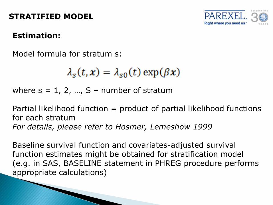
STRATIFIED MODEL Estimation: Model formula for stratum s: where  s  =  1,  2,  …,  S  – number of stratum Partial likelihood function = product of partial likelihood functions for each stratum For details, please refer to Hosmer, Lemeshow 1999 Baseline survival function and covariates-adjusted survival function estimates might be obtained for stratification model (e.g. in SAS, BASELINE statement in PHREG procedure performs appropriate calculations)

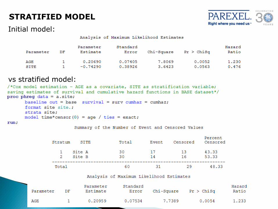
STRATIFIED MODEL Initial model: vs stratified model:

CONCLUSIONS Fit statistics comparison: Computational time comparison (in seconds):

CONCLUSIONS Overall assessment – linear predictor method

CONCLUSIONS In general: Accounting for the fact that proportional hazard assumption

is violated provides more detailed results as compared with initial model

Interaction with time: enables to analyze how HR changes over time provides parameter estimates for variable for which PH assumption is violated might require more computational resources than stratified model (Allison, 1995)

Stratified model: requires less computational resources enables to obtain baseline and covariates-adjusted survival function estimate for each stratum

does not provide parameter estimate for stratification variable

Thank you for your attention!