External Economies of Scale and International Trade: Further Analysis Kar-yiu Wong 1 University of Washington August 9, 2000 1 Department of Economics, Box 353330, University of Washington, Seattle, WA 98195- 3330, U. S. A.; Tel. 1-206-685-1859; Fax: 1-206-685-7477; e-mail: [email protected]; http://faculty.washington.edu/karyiu/
Transcript
External Economies of Scale and InternationalTrade: Further Analysis
Kar-yiu Wong1
University of Washington
August 9, 2000
1Department of Economics, Box 353330, University of Washington, Seattle, WA 98195-3330, U. S. A.; Tel. 1-206-685-1859; Fax: 1-206-685-7477; e-mail: [email protected];http://faculty.washington.edu/karyiu/
Abstract
This paper examines the validity of the ¯ve fundamental theorems of internationaltrade and some other issues in a general model of externality. The model allows thepossibility of own-sector externality and cross-sector externality. This paper derivesconditions under which some of these theorems are valid, and explains what thegovernment may choose to correct the distortionary e®ects of externality. Conditionsunder which a economy with no optimality policies may gain from trade are alsoderived.
c° Kar-yiu Wong
1 Introduction
Ever since the work of Marshall (1879, 1890), external economies of scale has been animportant topic in the economics literature. Marshall considered economies of scaleexternal to ¯rms while the ¯rms remained competitive. This assumption providesa °exible model that is compatible with perfect competition while it can be usedto handle variable returns to scale. Models of external economies of scale are alsocommon in the theory of international trade.1 However, most of the results obtainedare mixed and are sensitive to the structures of the models assumed. In most cases,people limit their analysis to some special cases, and derive results that may or maynot be generalized.2
Wong (2000b, 2000c) develop a basic, two-factor, two-sector model of externaleconomies of scale. It has externality in one sector, but no cross-sector externalityis assumed. The advantage of the model is that it is di®erent from the neoclassicalframework in only one aspect. Thus the results derived from the model can be com-pared with the well known results in the neoclassical framework, and any di®erencecan be attributed to the existence of external economies of scale. Another advan-tage of the present model is that it reduces to some more special cases consideredin the literature: the case of one factor and the case of two countries with the samecapital-labor ratio but di®erent sizes.It is recognized that the basic model has its own limitations, and some of the
results may not be valid in a more general model. It is thus the purpose of this paperto examine the implications of relaxing some of the assumptions in the basic model.The model considered in the present paper has externality in both sectors and
cross-sector externality between the sectors. This means that an increase in the outputin one of the sectors will have a feedback e®ect on its output and also will a®ect theoutput of the other sector (in addition to the e®ects due to reallocation of resources).As a result, e®ects of externality on resource allocation, income distribution, andforeign trade will no longer be so pure, as in general several forces may occur at thesame time. Therefore we cannot expect to have results as clean as those obtained inthe basic model.The purpose of developing the present more general model is to see how much
we can say about foreign trade when both own-sector externality and cross-sectorexternality are present. Perhaps one may say that in such a general model anythingcan happen. However, as shown in this paper, there are cases in which de¯nite results
1See Wong (2000a) for an introductory note on externality and international trade.2A general model has been examined in Tawada (1989).
1
can be obtained.As is done in Wong (2000b), we will examine the validity of the ¯ve fundamental
theorems of international trade, but we are also using the present model to derivemore implications of externality. Noting that externality is a form of distortion,meaning that a competitive equilibrium in the absence of any corrective policies is ingeneral suboptimal, we do two more things in the present paper: deriving the optimaltax-cum-subsidy policies to correct the distortion, and analyzing the gains from tradewhen no corrective policies have been imposed. The results we will derive are moregeneral than those in the literature.Section 2 of the present paper introduces the model and its basic features. The
virtual system technique in analyzing comparative static results is also introduced.Section 3 derives the output e®ects of an increase in factor endowments. The validityof the Rybczynski Theorem will be discussed. Section 4 turns to the relationshipbetween commodity prices and factor prices, with a careful examination of the validityof the Stolper-Samuelson Theorem. Autarkic equilibrium is examined in Section5, where the optimal policy will be derived. Section 6 allows international tradebetween two countries with identical technology and preferences, but the countriesmay have di®erent factor endowments. The validity of the Law of ComparativeAdvantage, the Heckscher-Ohlin Theorem and the Factor Price Equalization Theoremwill be examined. Section 7 analyzes the gains from trade for one or both economies.Su±cient conditions for a gainful trade will be derived. The last section concludes.
2 The Model
The model examined in the present paper is a general version of the basic model ofexternality introduced in Wong (2000b, 2000c). The present model is used to examinehow some of the results derived in Wong (2000b) may or may not survive in a moregeneral model. In particular, we will examine whether the ¯ve fundamental tradetheorems are still valid. The model will also be used to derive more properties ofexternality that have not been examined in Wong (2000b). In this section, we brie°ydescribe the model and explain how it is di®erent from the basic model.
2.1 Production Technology
There are two countries, but for the time being, we focus on the home economy. Thereare two goods, labeled 1 and 2, and two factors, capital and labor. The technology
2
of sector i; i = 1; 2, is described by the following production function:
Qi = hi(Q1; Q2)Fi(Ki; Li); (1)
where Qi is the output of sector i; and Ki and Li are the capital and labor inputsemployed in the sector. Function hi(Q1; Q2) measures the externality e®ect. Firmsin sector i regard the value of the function as constant, but in fact it depends on theaggregate output levels of the sectors. The argument Qi in function hi(:; :) measuresthe own-sector externality e®ect while Qk; i 6= k; represents the cross-sector exter-nality e®ect. Function Fi(:; :) is increasing, di®erentiable, linearly homogeneous, andconcave. We assume that sector 1 is capital intensive at all possible factor prices.Denote the supply price of sector i by psi :Let us de¯ne the following elasticities of function hi(:; :)
"ij ´ @hi@Qj
Qjhi= hij
Qjhi; i; j = 1; 2;
where hij ´ @hi=@Qj: The own-sector elasticity of sector i; "ii; is sometimes calledthe sector's rate of variable returns to scale. The sign of hij ; or that of "ij ; representshow a change in the output of good j may a®ect hi(:; :): For example, if "ii > 0;sector i is subject to increasing returns; if "ij > 0; i 6= j; then an increase in theoutput of good j will have a positive externality on the production of good i: Thecurrent model reduces to some special cases. For example, if "12 = "21 = "22 = 0 forall output levels, it reduces to the basic model in which only externality in sector 1exists with no cross-sector externality.The rest of the model has the usual properties of a neoclassical framework; for
example, all sectors are competitive and there are perfect price °exibility and perfectfactor mobility across sectors. In the present framework, full employment of factorsis achieved
K = K1 +K2 (2)
L = L1 + L2; (3)
where K and L are the available amounts of capital and labor in the economy, andare assumed to be given exogenously.
2.2 Marginal Products of Factors
Since the ¯rms in the two sectors take the value of hi = hi(Q1; Q2) as given, theprivate marginal product (PMP) of factor j in sector i; i = 1; 2, j = K; L; is equal to
PMPij = hiFij(Ki; Li); (4)
3
where Fij(Ki; Li) is the partial derivative of Fi with respect to factor j: The privatemarginal products are what ¯rms consider in choosing the optimal employment ofthe factors in maximizing their pro¯ts. However, the PMP is evaluated under theassumption that the aggregate output levels of the two sectors remain unchanged.That is not true for each sector or the economy. Thus we can derive the total e®ectof an increase in factor j on the output of sector i by totally di®erentiating theproduction functions:
Qij = FihiiQij ¡ FihikQkj + hiFij ; (5)
for i; k = 1; 2, i 6= k; j = K; L: In deriving (5), the full employment conditionshave been used to give dK1+ dK2 = 0; and dL1+ dL2 = 0: Alternatively, (5) can bewritten as
Qi = "iiQi + "ikQk + ºijbji; (6)
where ºij = jFij=Fi is the elasticity of function Fi(:; :) with respect to factor j;j = K;L: Note that ºij has the same sign as the PMP of factor j in sector i; which ispositive when competitive ¯rms are maximizing their pro¯ts. If we de¯ne Áj = j1=j2and use the full employment condition, (6) can be written in a matrix form:"
1¡ "11 ¡"12¡"21 1¡ "22
#"Q1
Q2
#=
"º1j
¡Ájº2j
#bj1: (7)
Let £ = (1¡ "11)(1¡ "22)¡ "12"21 be the determinant of the matrix in (7), which canbe solved to give
Q1 =º1j(1¡ "22)¡ º2j"12Áj
£bj1 (8)
Q2 =º2j(1¡ "11)¡ º1j"21=Áj
£bj2: (9)
The social marginal product (SMP) of factor j in sector i is the total derivative ofoutput Qi with respect to the factor. In other words, using (8) and (9), the socialmarginal product of factor j in sector i; k is equal to
Qij =hi(1¡ "kk)
£Fij ¡ Fihkhik
£Fkj ; (10)
for i 6= k: In general, the social marginal product of a factor is not the same as itsprivate marginal product. Consider the following condition:
4
Condition A. 1¡ "ii > 0 ¸ "ik; and (1¡ "11)(1¡ "22) > "12"21; i 6= k:
Lemma 1. Given condition A, the social marginal product of labor or capital inany sector is positive.
The lemma can be proved by using (8) and (9). Condition A is a su±cientcondition for positive social marginal products. It appears to be restrictive, butgenerally what it requires is that the externality terms are not too signi¯cant inmagnitudes.Note that the relationship between the e±cient outputs in the present model can
be described by the production possibility frontier, which is negatively sloped, but itscurvature is in general ambiguous.
2.3 The Virtual and Real Systems
Following Wong (2000b), we introduce the concept of virtual and real systems. In thevirtual system, we de¯ne ~Qi as the virtual output, which is equal to ~Qi = Fi(Ki; Li)with the later function described in (1). Since function Fi(:; :) has the propertiesof a neoclassical production function, the virtual system behaves like a neoclassicalframework. The advantage of the present approach is that the properties of theneoclassical framework are well known.Let us denote the price of sector i in the virtual system by ~pi. As it is done for the
neoclassical framework, the virtual output of sector i can be expressed as a functionof virtual prices and factor endowments:3 ~Qi = ~Qi(~p1; ~p2; K;L). The virtual outputof sector i is related to the real output in the following way:
Qi = hi(Q1; Q2) ~Qi(~p1; ~p2; K;L): (11)
Similarly, the virtual prices are related to the real prices in the following way:
~psi = hi(Q1; Q2)psi : (12)
Conditions (11) and (12) give the relationship between the virtual and real systems.The approach we take in this paper is to make use of the properties of the neoclassicalframework and then apply conditions (11) and (12) to derive the properties of thereal system.
3We can de¯ne a virtual GDP (gross domestic product) function. Partial di®erentiation of thefunction with respect to virtual prices gives the virtual output function. See Wong (1995) for moredetails.
5
The e±cient virtual outputs can be described by a virtual production possibilityfrontier, which is negatively sloped and concave to the origin. For the analysis below,the frontier is assumed to be strictly concave to the origin.The output function in (11) can be used to de¯ne the following elasticities:
´ik =@ ~Qi@~pk
~pk~Qi:
3 Output E®ects
In this section, we examine the validity of the two fundamental trade theorems in thepresent framework: the Rybczynski Theorem and the Stolper-Samuelson Theorem.
3.1 General Conditions
Di®erentiate conditions (11) and (12) totally and rearrange the terms to give
dQi = hii ~QidQi + hij ~QidQj + hi[ ~Qiid~psi + ~Qijd~p
sj + ~QiKdK + ~QiLdL] (13)
d~psi = hiipsidQi + hijp
sidQj + hidp
si ; (14)
where i 6= j: Combining together equations (13) and (14), we have'iidQi + 'ijdQj = h
2i~Qiidp
si + hi
~Qijhjdpsj + hi
~QiKdK + hi ~QiLdL; (15)
where
'ii = 1¡ hii ~Qi ¡ hi ~Qiihiipsi ¡ hi ~Qijhjipsj'ij = ¡(hij ~Qi + hi ~Qiihijpsi + hi ~Qijhjjpsj):
Let us introduce the following elasticities:
´ij =@ ~Qi@~psj
~psj~Qi=hihj ~Qijp
sj
~Qi
´im =@ ~Qi@m
m~Qi=him ~Qim~Qi
;
where i; j 2 f1; 2g; and m 2 fK;Lg: From the properties of the neoclassical frame-work, we know that ~Qij > 0 for i = j; or < 0 for i 6= j: This implies that ´ij > 0
6
if i = j; or < 0 if i 6= j: Furthermore, due to the factor-intensity ranking assumed,´1K; ´2L > 0; and ´2K ; ´1L > 0: Using the homogeneity properties of the virtual GDPfunction, we can easily derive the following relations:
´ii + ´ij = 0 (16)
si´ii + sj´ji = 0 (17)
´iL + ´iK = 1; (18)
where si ´ ~pi ~Qi=g is the share of sector i; and g is the value of the GDP of theeconomy.4 Let us de¯ne ¸mi as the proportion of factor m employed in sector i; andj¸j ´ ¸K2 ¡ ¸L2 ´ ¸L1 ¡ ¸K1: Since sector 1 is capital intensive, j¸j < 0: We knowfurther that
´im = »im¸njj¸j ; (19)
where i; j = 1; 2; m; n = K;L; i 6= j; m 6= n; and »im is an index which is equal to 1for (i = 1 and m = L) or (i = 2 and m = K); or equal to ¡1 for (i = 2 and m = L)or (i = 1 and m = K):5
Let us use a \hat" to denote the proportional change of a variable; for example,Qi ´ dQi=Qi: Using the output elasticities, (15) can be written in an alternative way:
®iiQi + ®ijQj = ´iipsi + ´ijp
sj + ´iKK + ´iLL; (20)
where
®ii = 1¡ "ii ¡ ´ii"ii ¡ ´ij"ji (21)
®ij = ¡("ij + ´ii"ij + ´ij"jj); i 6= j: (22)
In (21) and (22), the signs of ®ii and ®ij are in general ambiguous. In the neoclassicalframework, "ik = 0; i; k = 1; 2: This implies that ®ii = 1 and ®ij = 0; for i 6= j: Forthe two sectors, equation (20) can be expressed in an alternative form:"
®11 ®12
®21 ®22
#"Q1
Q2
#=
"´11
´21
#ps1 +
"´12
´22
#ps2 +
"´1K
´2K
#K +
"´1L
´2L
#L:
(23)
4It can be shown that, based on the assumed factor intensity ranking,
¸K1¸K2
>s1s2>¸L1¸L2
:
Since this result is not needed in the present paper, its proof is left to the reader.5For the proof of these results, see Wong (1995, Chapter 2).
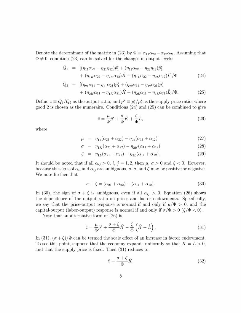
De¯ne z ´ Q1=Q2 as the output ratio, and ps ´ ps1=ps2 as the supply price ratio, wheregood 2 is chosen as the numeraire. Conditions (24) and (25) can be combined to give
It should be noted that if all ®ij > 0; i; j = 1; 2; then ¹; ¾ > 0 and ³ < 0. However,because the signs of ®ii and ®ij are ambiguous, ¹; ¾; and ³ may be positive or negative.We note further that
Condition (32) represents the scale e®ect of an increase in factor endowments on theoutput ratio.Conditions (27) to (30) consist of the following two terms: (®11+®12) and (®21+
®22): Let us for the time being focus on these two terms. Making use of (21) and(22), we have
Condition (38) means that the scale e®ect is zero if "11 + "12 = "21 + "22: Considerthe following condition:
Condition B. "11 + "12 > "21 + "22:
Lemma 2. Given condition A, ¹ > 0: Given conditions A and B, ¾; ¾ + ³ > 0 and³ < 0:
This lemma can be proved easily by making use of equations (35) to (38). Notethat condition A is su±cient for ¹ to be positive.
9
3.2 Production Stability
As Wong (2000b) shows, comparative statics e®ects can be analyzed both in a lo-cal and a global ways. To analyze global changes, we need to examine stabilityof equilibrium and the adjustment process. Following Wong (2000b), we adopt theIde-Takayama rule (Ide and Takayama, 1991):
_z = ¯(¹p¡ ps) = Á(z); (39)
where ¯ > 0 is a constant, and ¹p is the supply price ratio the ¯rms are facing. Makinguse of (26), both sides of (39) are di®erentiated to give
libria is misplaced (a) because an unstable equilibrium is nearly never observed, and(b) because even if initially the system is at an unstable equilibrium, after a smalldisturbance the system will adjust to a stable equilibrium. In the present more gen-eral model, can these two results still exist? The answer is in the a±rmative. Forexample, suppose that the initial equilibrium is at B, with the output ratio at zB.Consider a small disturbance that lowers the output ratio to, say, zB0: Because the
We now make use of the adjustment rule introduced to analyze factor-output re-sponses. Let us focus on the e®ects of an increase in the capital endowment, as thee®ects of an increase in labor endowments can be analyzed in the same way. If wekeep z constant, the relationship between ps and K is given by a shift of the supplyprice schedule as a result of an increase in the capital endowment. In particular, therelationship is given by the following condition
in the supply price and the capital endowment is not clear. In the following table, weconsider all possibilities.Table 1 shows the types of price-output response, capital-output response, local
7This is what Samuelson (1949) called the Correspondence Principle. For more details, see Wong(2000b). See Samuelson (1971) for the Global Correspondence Principle.
1 + + + n n n n (a)2 + + ¡ n p p p (b)3 + ¡ + p p n p (d)4 + ¡ ¡ p n p n (c)5 ¡ + + p n p n (c)6 ¡ + ¡ p p n p (d)7 ¡ ¡ + n p p p (b)8 ¡ ¡ ¡ n n n n (a)
n = normal response; p = perverse response
Table 1: Output Responses to Prices and Capital Endowments
response indicates that the Rybcyznski e®ect holds.8 As shown in Table 1, the Ryb-cyznski e®ect is not guaranteed. In the present basic model, it is argued that if ¯nitechanges are allowed, the Rybcyznski e®ect will hold globally even if it is not locally.We now examine whether such results are still true. Column (8) of Table 1 showsthat they are no longer true: In fact, they are true in four of the eight cases only:cases 1, 4, 5, and 8. Alternatively, we say that they are true only in panels (a) and(c) of Figure 2.Let us examine these cases more carefully. Suppose that the exogenously given
price ratio is p1; with the initial equilibrium at point A or B, at which the price lineat p1 cuts the initial (solid) supply price schedule. In panel (a) of Figure 2, whichdescribes cases 1 and 8 in Table 1, the supply schedule is positively sloped, and anincrease in the capital stock shifts the schedule down, lowering the supply price at
8This means that a small increase in capital will induce a local increase in the output of good 1relative to good 2.
12
the same output ratio (point F), while the equilibrium point shifts from A to A0,implying an increase in the output ratio. This means that the local capital-outputresponse is normal. In fact, the capital-output response is also true in a global sense.This is because a drop in the supply price (to a level represented by F) will, by theadjustment rule (39), encourage an increase in the output of good 1, i.e., a rise inz: In panel (c), the local capital-output response is perverse (a drop in the outputratio from B to B0), but the global capital-output response is normal. The reason isthat the drop in the supply price ratio will induce an increase in the output ratio,shifting the equilibrium point B to the right, not to the left, until a stable equilibriumis reached.Panels (b) and (d) of Figure 2 represent two opposite cases. In panel (d), an
increase in the capital stock shifts the supply price schedule up, and the equilibriumpoint to the right from B to B0. Thus locally the capital-output response is normal.However, an upward shift of the supply price schedule implies a drop in the outputratio until a stable equilibrium with a lower output ratio is reached. Panel (b),however, shows a case in which the capital-output response is not normal both locallyand globally.Table 1 and Figure 2 reveal the following results:
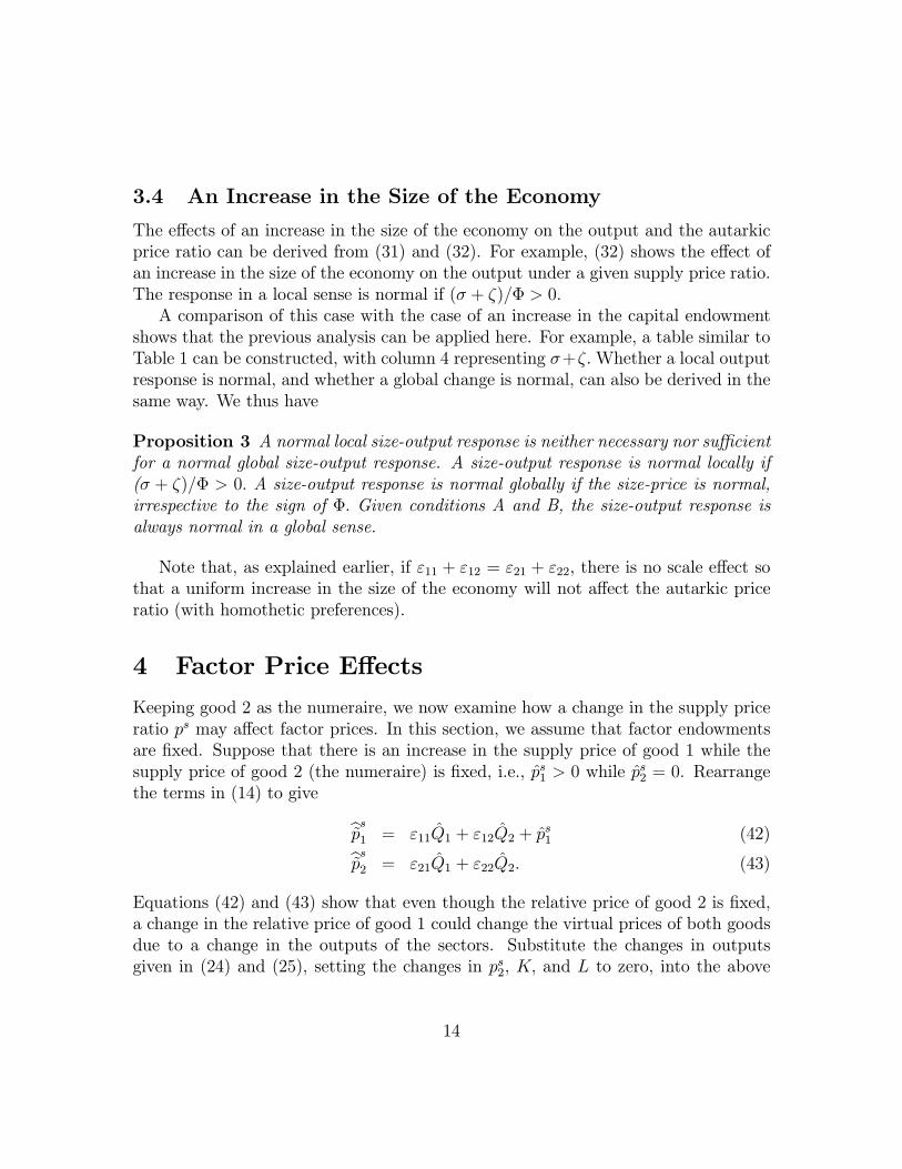
shows that the previous analysis can be applied here. For example, a table similar toTable 1 can be constructed, with column 4 representing ¾+³:Whether a local outputresponse is normal, and whether a global change is normal, can also be derived in thesame way. We thus have
Note that, as explained earlier, if "11 + "12 = "21 + "22; there is no scale e®ect sothat a uniform increase in the size of the economy will not a®ect the autarkic priceratio (with homothetic preferences).
4 Factor Price E®ects
Keeping good 2 as the numeraire, we now examine how a change in the supply priceratio ps may a®ect factor prices. In this section, we assume that factor endowmentsare ¯xed. Suppose that there is an increase in the supply price of good 1 while thesupply price of good 2 (the numeraire) is ¯xed, i.e., ps1 > 0 while p
Equations (42) and (43) show that even though the relative price of good 2 is ¯xed,a change in the relative price of good 1 could change the virtual prices of both goodsdue to a change in the outputs of the sectors. Substitute the changes in outputsgiven in (24) and (25), setting the changes in ps2; K; and L to zero, into the above
Equations (44) and (45) show explicitly how a change in the real prices of the goodscould a®ect their virtual prices. This result has the following implications on thecorresponding changes in factor prices.
Lemma 3. If own-sector externalities are non-negative while cross-sector external-ities are non-positive ("ii ¸ 0 and "ij · 0; i; j = 1; 2; i 6= j); and if ®ij ¸ 0 fori; j = 1; 2; with at least one inequality, then ±1 ¸ 1; ±2 · 0.
Lemma 3 follows immediately from the de¯nitions of ±1 and ±2: Note that if ®ij = 0for all i; j = 1; 2; then ±1 = 1 and ±2 = 0: From (44) and (45), Lemma 3 implies thatgiven the conditions stated an increase in the relative price of good 1 will raise thevirtual relative price of good 1 but lower (or not raise) the virtual relative price ofgood 2.De¯ne the unit cost function of sector i in the virtual system by ci(w; r); i = 1; 2;
which is linearly homogeneous, di®erentiable, and concave. With positive outputs ofboth goods, the cost-minimization conditions are
ci(w; r) = ~psi : (46)
Di®erentiate both sides of (46), rearrange terms, and make use of (42) and (43) toyield "
#1L #1K
#2L #2K
#"w
r
#=
"±1
±2
#ps1; (47)
where #ij is the elasticity of unit cost function of sector i with respect to the price offactor j: The determinant of the matrix in (47) is equal to D = #1L#2K¡#2L#1K < 0;
15
where the sign is due to the assumed factor intensity ranking.9 The equation is thensolved for the changes in factor prices
w =±1#2K ¡ ±2#1K
Dps1 (48)
r =±2#1L ¡ ±1#2L
Dps1: (49)
Conditions (48) and (49) immediately give the following proposition:
Proposition 4 The Stolper-Samuelson Theorem in the presence of external economiesof scale is valid if condition A holds and if all ®ij > 0; i; j = 1; 2:
It should be noted that in the above proposition, when given condition A and theassumption that all ®ij > 0; w=ps1 < 0 and r=ps1 > 1: To see the later inequalities,
note that in the virtual system, r=b~ps1 > 1; and by Lemma 1 b~ps1=ps1 > 1:5 Autarkic Equilibrium
To derive the autarkic equilibrium, we assume that the preferences of the home econ-omy is described by a social utility function, which is homothetic, increasing, di®eren-tiable, and quasi-concave. Homotheticity of the preferences means that the demandprice ratio, with good 2 as the numeraire, can be expressed as a function of theconsumption ratio, pd = °(z); where the derivative °0(z) is negative. Let the priceelasticity of demand be denoted by ± ´ ¡z=pd:
5.1 Equilibrium Conditions
The autarkic equilibrium is described by an output ratio that equalize the supplyprice and the demand price, i.e.,
ps = pd = pa; (50)
where the superscript \a" denotes the autarkic value of a variable. Conditions (50)and (26) can be combined together to give
pa = ¡µh¾K + ³L
i; (51)
9We have used Shephard's lemma that @ci=@w = Li= ~Qi and @ci=@r = Ki= ~Qi:
Thus, a small increase in the capital stock will lower the autarkic price ratio if sign(µ)= sign(¾):We say that in this case the response of the autarkic price ratio is normal.On the other hand, if ¾ > 0 under the conditions mentioned in Lemma 2, then,as argued in Wong (2000b), an increase in the capital stock will lower in a globalsense the autarkic price ratio, whether or not µ is positive. Similar conclusion can bereached for an increase in the labor endowment, or a uniform increase in the size ofthe economy.Thus we have
Proposition 5 A locally normal response of the autarkic price ratio to an increasein the endowment of either capital or labor, or to a uniform increase in the size ofthe economy, is neither necessary nor su±cient for a globally normal response of theautarkic price ratio to an increase in the capital stock. Given conditions A and B, theresponse of the autarkic price ratio to an increase in the factor endowment is globallynormal.
5.2 Optimal Policy
Externality in the present model represents a distortion. This means that a marketequilibrium in general is not optimal in terms of the welfare of the economy. From thedescription of the model given in Section 2, it is clear that externality is due to theassumption that the ¯rms ignore the indirect e®ect of an increase in the employmentof a factor on function hi(Q1; Q2): As a result, there is a divergence between theprivate marginal product and social marginal product of a factor.10
The optimal policy considered here is a set of taxes/subsidies imposed on theemployment of factors. We argue that the optimal policy on sector i consists of an
10For more discussion about private marginal product and social marginal product, see Wong(2000a).
17
ad valorem employment subsidy si plus a lumpsum subsidy of Ái on factor j; where
si ="ii(1¡ "kk) + "ik"ki
£(53)
Ái = ¡piµhkFihikFkj
£
¶; (54)
where i; k = 1; 2, i 6= k; j = K; L; and the variables are evaluated at the optimalpoint. Note that a negative subsidy is a tax.To see how this policy works, let us consider the income of labor. The e®ective
wage rate consists of three parts: the payment by a ¯rm, the employment subsidyfrom the government, and the lumpsum subsidy. The ¯rms take the subsidies asgiven, and keep on ignoring the externality e®ects, i.e., they pay the factors theyemploy according to their private marginal products. The total income of a worker,which is regarded as the e®ective wage rate, is equal to
w = pi(1 + si)hiFiL + Ái: (55)
To ¯nd out what this wage rate is, we note that
1 + si =1¡ "kk£
: (56)
Substituting (56) into (55) and using (53) and (54), we have
w = piQiL (57)
for i = 1; 2. Condition (57) means that the wage rate is equal to value of socialmarginal product of labor. A similar condition can be derived for the rental rate.Thus in the presence of the present policy, both factors are employed optimally.
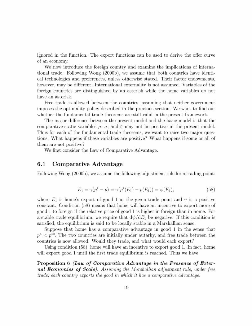
6 International Trade
We now consider open economies and analyze foreign trade. In order to have mean-ingful comparison of the two countries, we assume that the autarkic equilibrium ofeach country is unique. As it is done in Wong (2000b), denote the export supplyof good 1 of home by E1(p;K;L); where p is the domestic price ratio of good 1.Note that both K and L are treated as exogenous. Invert the export supply functionE1 = E1(p;K;L) to give p = ½(E1); where for simplicity the factor endowments are
18
ignored in the function. The export functions can be used to derive the o®er curveof an economy.We now introduce the foreign country and examine the implications of interna-
tional trade. Following Wong (2000b), we assume that both countries have identi-cal technologies and preferences, unless otherwise stated. Their factor endowments,however, may be di®erent. International externality is not assumed. Variables of theforeign countries are distinguished by an asterisk while the home variables do nothave an asterisk.Free trade is allowed between the countries, assuming that neither government
imposes the optimality policy described in the previous section. We want to ¯nd outwhether the fundamental trade theorems are still valid in the present framework.The major di®erence between the present model and the basic model is that the
comparative-static variables ¹; ¾; and ³ may not be positive in the present model.Thus for each of the fundamental trade theorems, we want to raise two major ques-tions. What happens if these variables are positive? What happens if some or all ofthem are not positive?We ¯rst consider the Law of Comparative Advantage.
6.1 Comparative Advantage
Following Wong (2000b), we assume the following adjustment rule for a trading point:
_E1 = °(p¤ ¡ p) = °(½¤(E1)¡ ½(E1)) = Ã(E1); (58)
where E1 is home's export of good 1 at the given trade point and ° is a positiveconstant. Condition (58) means that home will have an incentive to export more ofgood 1 to foreign if the relative price of good 1 is higher in foreign than in home. Fora stable trade equilibrium, we require that dÃ=dE1 be negative. If this condition issatis¯ed, the equilibrium is said to be locally stable in a Marshallian sense.Suppose that home has a comparative advantage in good 1 in the sense that
pa < p¤a: The two countries are initially under autarky, and free trade between thecountries is now allowed. Would they trade, and what would each export?Using condition (58), home will have an incentive to export good 1. In fact, home
will export good 1 until the ¯rst trade equilibrium is reached. Thus we have
Proposition 6 (Law of Comparative Advantage in the Presence of Exter-nal Economies of Scale). Assuming the Marshallian adjustment rule, under freetrade, each country exports the good in which it has a comparative advantage.
19
This proposition is the same as the one in Wong (2000b), which means that thelaw stays as the model becomes more general with externality in both sectors andwith cross-sector externality. The intuition is clear: this law does not depend on thesigns of the comparative-static variables.Of course, it should be noted that the law stated above is weaker than the Law
of Comparative Advantage in the neoclassical framework.
6.2 The Heckscher-Ohlin Theorem
Wong (2000b) shows that in the basic model of externality, a certain form of theHeckscher-Ohlin Theorem exists. The result depends on the fact that in the model ¹;¾; and ¾+³ > 0 while ³ < 0: In particular, it was shown that home has a comparativeadvantage in good 1 if it has more capital or is bigger uniformly, and has a comparativein good 2 if it is abundant absolutely in labor. This result does not depend on the signof µ at the autarkic point because comparing the factor endowments of the countries,which are much di®erent from each other, is the same as considering global changesin comparative static analysis.In the present model, all these comparative static variables may not have the
\right" sign; for example, we may have ¹ < 0 and ¾ > 0:What can we say about thecomparative advantages of the countries and their patterns of trade?This question can be answered by using Table 1, which shows the e®ects of an
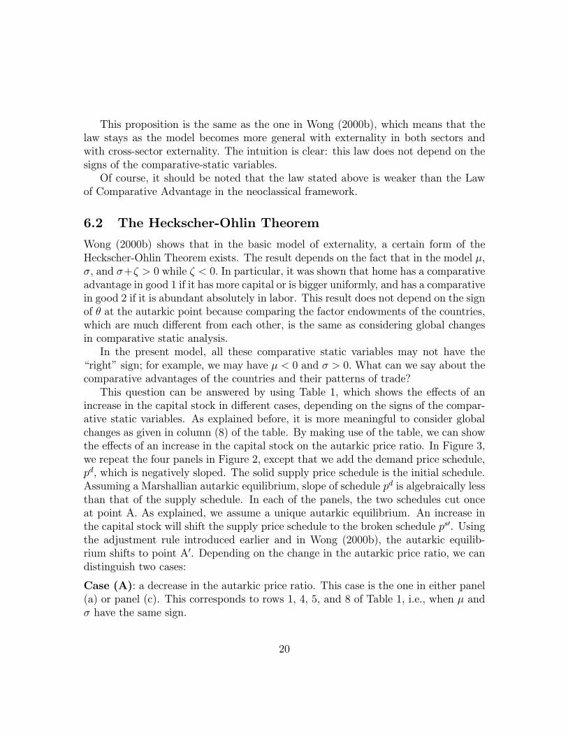
increase in the capital stock in di®erent cases, depending on the signs of the compar-ative static variables. As explained before, it is more meaningful to consider globalchanges as given in column (8) of the table. By making use of the table, we can showthe e®ects of an increase in the capital stock on the autarkic price ratio. In Figure 3,we repeat the four panels in Figure 2, except that we add the demand price schedule,pd; which is negatively sloped. The solid supply price schedule is the initial schedule.Assuming a Marshallian autarkic equilibrium, slope of schedule pd is algebraically lessthan that of the supply schedule. In each of the panels, the two schedules cut onceat point A. As explained, we assume a unique autarkic equilibrium. An increase inthe capital stock will shift the supply price schedule to the broken schedule ps0. Usingthe adjustment rule introduced earlier and in Wong (2000b), the autarkic equilib-rium shifts to point A0. Depending on the change in the autarkic price ratio, we candistinguish two cases:
Case (A): a decrease in the autarkic price ratio. This case is the one in either panel(a) or panel (c). This corresponds to rows 1, 4, 5, and 8 of Table 1, i.e., when ¹ and¾ have the same sign.
20
Case (B): an increase in the autarkic price ratio. This case is shown in either panel(b) or panel (d), and corresponds to rows 2, 3, 6, and 7 | ¹ and ¾ having di®erentsigns.
The table and the analysis can be applied to the other two variables, ¾ + ³ and³: In the basic model, these comparative static variables are of the \right" sign, i.e.,¹; ¾; ¾ + ³ > 0 while ³ < 0: One important result is that a modi¯ed version of theHeckscher-Ohlin Theorem is valid. In the present model, these variables are of the\right" sign under certain conditions. Thus we have,
Proposition 7 (Heckscher-Ohlin Theorem in the Presence of ExternalEconomies of Scale). When given conditions A and B, a country exports thecapital-intensive good if it is relatively and absolutely abundant in capital, or if it isuniformly bigger.
6.3 Factor Price Equalization
We now turn to the factor prices in the two countries under free trade. We keepthe usual assumptions for the Theorem of Factor Price Equalization, including (a)equalized commodity prices (due to free trade and no transport costs) and (b) diver-si¯cation in production.Note that the virtual system behaves like the neoclassical framework, meaning
that a necessary condition for factor price equalization is that the virtual commodityprices be the same in both countries. Recall that the virtual commodity prices arerelated to the (real) commodity prices as follows:
~pi = hi(Q1; Q2)pi: (59)
Assuming that hik 6= 0 in the general case, the two equations represented by (59)imply that in order to have the same virtual commodity prices in the countries, thecountries must have the same output levels of the two goods. However, since thecountries have identical technologies, and since they are facing the same commodityprices, they need to have the same factor endowments. As a result, the only possibilityis that the two countries are identical not only in technologies and preferences, butalso in factor endowments. In this case, when the countries allow free trade, no tradeis an equilibrium, but the no-trade equilibrium can be either stable or unstable. Ifthe equilibrium is unstable, a shock will move the countries from the equilibrium toa free-trade equilibrium, with one of the countries exporting good 1. However, thecountry that exports (imports) good 1 must produce more (less) good 1 than that inthe other countries. Thus we have
21
Proposition 8 When the countries trade, generally factor prices are not equalizedunder free trade.
It should be noted that the Factor Price Equalization Theorem in the neoclassicalframework does not require identical preferences across countries. This is also truefor the basic model of externality introduced in Wong (2000b). In the above analysis,we begin with the assumption that the countries have identical technologies and alsopreferences, and show that the theorem in general is not valid. This result, which isnegative in a sense, holds whether the countries have identical preferences.
7 Gains from Trade
Externality is a form of distortion, which means that a market equilibrium in theabsence of any government intervention is suboptimal. It is therefore not surprisingto ¯nd that an economy with externality may have a lower welfare under free tradethan under autarky.There has been a lot of work that derives su±cient conditions for a gainful trade
in the presence of external economies of scale.11 It has been pointed out that externaleconomies of scale creates distortion on the production side of the economy while theconsumption side is free from distortion. This means that the consumption gain fromtrade of the economy is non-negative while the production gain from trade may benegative.12 Therefore a su±cient condition for a gainful trade is that the productiongain is positive (or non-negative if the consumption gain is positive). The literatureis characterized by work on determining conditions under which the production gainis non-negative.Keeping on using subscript \a" to denote autarkic values of variables, and using
no subscripts for the variables' values under free trade, the production gain is de¯nedas:
PG =2Xi=1
piQi ¡2Xi=1
piQai : (60)
11See Wong (1995, Chapter 9) for a recent survey and discussion.12The consumption gain is positive if there is a change in the commodity price ratios and if there
are consumption substitution possibilities.
22
Substitute the production function in (1) into (60), we get
PG =2Xi=1
pihi(Q1; Q2) ~Qi ¡2Xi=1
pihi(Qa1; Q
a2) ~Q
ai
=2Xi=1
~pi ~Qi ¡2Xi=1
pihai~Qai : (61)
where hai = hi(Qa1; Q
a2): Because the virtual system behaves like a neoclassical frame-
work, its production gain measured in terms of virtual prices and outputs is non-negative, i.e.,
2Xi=1
~pi ~Qi ¸2Xi=1
~pi ~Qai ;
or
2Xi=1
piQi ¸2Xi=1
pihi(Q1; Q2) ~Qai : (62)
Comparing (61) and (62), we can see that a su±cient condition for a non-negativeproduction gain is the following condition
2Xi=1
pihi(Q1; Q2) ~Qai ¸
2Xi=1
pihi(Qa1; Q
a2)~Qai : (63)
Various conditions analogous to (63) have been derived and applied in the literature.In the present model, when will condition (63) hold? One su±cient condition is that
hi(Q1; Q2) ¸ hi(Qa1; Qa2); (64)
for i = 1; 2. Another su±cient condition is to make use of function hi(:; :) andexamine how outputs of the sectors should change in order to guarantee condition(64). In the present two-sector model, one of the sectors must expand while the othersector shrinks as the economy shifts from the autarkic equilibrium to a free-tradeequilibrium.13 Consider the following condition:
13Free trade leads to a change in the production point if there is a change in the relative priceand production substitution is possible.
23
Condition G. For i; k = 1; 2; hkk and hik are either (a) zero or (b) the same signas (Qk ¡Qak):To interpret what condition G means, imagine that sector 1 expands, i.e., Q1 ¡
Qa1 > 0: Then we require that the sector is subject to increasing returns and it has apositive external e®ect on sector 2.
Lemma 4. Given condition G, condition (64) is satis¯ed.
Lemma 4 is intuitive. In order to satisfy (64), if a sector expands, then it musthave a positive externality on itself and also on the other sector, or if a sector shrinks,it must have a negative externality on itself and on the other sector. Using Lemma 4and the above analysis, we immediately have the following proposition:
Proposition 9 A su±cient condition for a gainful free trade is condition G.
Condition G is a strong one because it has restrictions on not just own-sectorexternality on both sectors but also on cross-sector externality. Note that in thespecial case in which cross-sector externality is absent, then condition G reduces to thefamous Kemp-Negishi condition (Kemp and Negishi, 1970): an economy gains fromtrade if the sector that is subject to increasing returns expands while the sector thatis subject to decreasing returns shrinks. In the presence of cross-sector externality,the Kemp-Negishi condition is not su±cient for a gainful trade.14
8 Concluding Remarks
This paper examines the implications of externality in a general model, in which bothown-sector externality and cross-externality may be present. This model reduces tothe basic model in Wong (2000b, 2000c) as a special case.It is of course not surprising that some of the results derived in Wong (2000b)
may not hold here. For example, four of the ¯ve trade theorems may not hold.These theorems are the Rybczynski Theorem, the Stolper-Samuelson Theorem, theHeckscher-Ohlin Theorem, and the Factor Price Equalization Theorem. The modi¯edLaw of Comparative Advantage, however, remains valid.15 The reason is that this law
14See Wong (1995, Chapter 9) for extension of the Kemp-Negishi results and a discussion ofrelevant work by other people.15Strictly speaking, the law proved in Wong (2000b) and the present paper is only half of what
is in the Law of Comparative Advantage derived in the neoclassical framework. The other half,that the free-trade world price ratio is bounded by the autarkic price ratios in the countries, is notnecessarily valid.
24
describes the relationship between autarkic price ratios and patterns of trade, and isnot a®ected by externality, or even the technologies in general, in the countries.16
As we showed, in general the results are ambiguous. We did ¯nd some su±cientconditions under which stronger results are valid.
16As a matter of fact, the Law of Comparative Advantage does not require identical technologyand/or preferences in the countries.
25
O
ps
z
K
L
M
N
A.. .
.A’B’
B
..
C
C’
.
p1
p2
p’
Price-Output Response
Figure 1
zBzB’
Capital-Output Response
Figure 2
ps
p1
z
. .
.
ps
p1
z
. ..
(a) (b)
ps
p1
z
...
(c)
ps
p1
z
.. .(d)
ps
’psps
’ps
ps
’ps ps’ps
A
A
F
’ A
F
A’
BB
G
’
G
B B’
Autarkic Price Response to An Increase in Capital
Figure 3
p
pd
z
..
z
..
(a) (b)
p
z
(c)
p
z
..
(d)
ps
’psps
’ps
ps
’ps ps
’ps
AA’
AA’
A
A’
p
pdpd
..A
A’
pdpd
References
[1] Ide, Toyonari and Akira Takayama (1991), \Variable Returns to Scale, Para-doxes, and Global Correspondence in the Theory of International Trade," inAkira Takayama, Michihiro Ohyama, and Hiroshi Ohta (eds.), Trade, Policy,and International Adjustments, San Diego: Academic Press, Inc.: 108{154.
[2] Kemp, Murray C. and Takashi Negishi (1970), \Variable Returns to Scale,Commodity Taxes, Factor Market Distortions and Their Implications for TradeGains," Swedish Journal of Economics, 72 (1): 1{11.
[3] Marshall, Alfred (1879), Pure Theory of Foreign Trade, reprinted by LondonSchool of Economics and Political Science, 1930.
[4] Marshall, Alfred (1890), Principles of Economics, 8th edition, London: Macmil-lan, 1920.
[5] Samuelson, Paul A. (1947), Foundation of Economic Analysis, Cambridge, Mass.:Harvard University Press.
[6] Samuelson, Paul A. (1971), \On the Trail of Conventional Beliefs about theTransfer Problem," in Jagdish N. Bhagwati et al. (eds.), Trade, Balance of Pay-ments and Growth: Papers in International Economics in Honor of Charles P.Kindleberger, Amsterdam: North-Holland, 327{351.
[7] Tawada, Makoto (1989), Production Structure and International Trade, Berlin:Springer-Verlag.
[8] Wong, Kar-yiu (1995), International Trade in Goods and Factor Mobility, Cam-bridge, Mass.: MIT Press.
[9] Wong, Kar-yiu (2000a), \Externality in the theory of International Trade: SomeBasic Concepts," mimeo, University of Washington.
[10] Wong, Kar-yiu (2000b), \Fundamental Trade Theorems under ExternalEconomies of Scale," mimeo, University of Washington.
[11] Wong, Kar-yiu (2000c), \International Trade and Factor Mobility under ExternalEconomies of Scale," mimeo., University of Washington.